An Algorithm for Streaming Differentially Private Data

Abstract

Much of the research in differential privacy has focused on offline applications with the assumption that all data is available at once. When these algorithms are applied in practice to streams where data is collected over time, this either violates the privacy guarantees or results in poor utility. We derive an algorithm for differentially private synthetic streaming data generation, especially curated towards spatial datasets. Furthermore, we provide a general framework for online selective counting among a collection of queries which forms a basis for many tasks such as query answering and synthetic data generation. The utility of our algorithm is verified on both real-world and simulated datasets.

1 Introduction

Many data driven applications require frequent access to the user’s location to offer their services more efficiently. These are often called Location Based Services (LBS). Examples of LBS include queries for nearby businesses (Bauer & Strauss, 2016), calling for taxi pickup (Lee et al., 2008; Zhang et al., 2012), and local weather information (Wikipedia contributors, 2017).

Much of location data contains sensitive information about a user in itself or when cross-referenced with additional information. Several studies (Jin et al., 2023) have shown that publishing location data is susceptible to revealing sensitive details about the user and simply de-identification (Douriez et al., 2016) or aggregation (Xu et al., 2017) is not sufficient. Thus, privacy concerns limit the usage and distribution of sensitive user data. One potential solution to this problem is privacy-preserving synthetic data generation.

Differential privacy (DP) can be used to quantifiably guarantee the privacy of an individual and it has been used by many notable institutions such as US Census (Abowd et al., 2019), Google (Erlingsson et al., 2014), and Apple (Team, 2017). DP has seen a lot of research across multiple applications such as statistical query answering (McKenna et al., 2021a), regression (Sarathy & Vadhan, 2022), clustering (Ni et al., 2018), and large-scale deep learning (Abadi et al., 2016). Privacy-preserving synthetic data generation has also been explored for various data domains such as tabular microdata (Hardt et al., 2012; Zhang et al., 2017; Jordon et al., 2019; Tao et al., 2021; McKenna et al., 2021b), natural language (Li et al., 2021; Yue et al., 2022), and images (Torkzadehmahani et al., 2019; Xu et al., 2019).

DP has also been explored extensively for various use cases concerning spatial datasets such as answering range queries (Zhang et al., 2016), collecting user location data (loc, 2021), and collecting user trajectories (Li et al., 2017). In particular for synthetic spatial microdata generation, a popular approach is to learn the density of true data as a histogram over a Private Spatial Decomposition (PSD) of the data domain and sample from this histogram (Zhang et al., 2016; Kim et al., 2018; Fanaeepour & Rubinstein, 2018; Qardaji et al., 2013). Our work also uses this approach and builds upon the method PrivTree (Zhang et al., 2016) which is a very effective algorithm for generating PSD.

Despite a vast body of research, the majority of developments in differential privacy have been restricted to a one-time collection or release of information. In many practical applications, the techniques are required to be applied either on an event basis or a regular interval. Many industry applications of DP simply re-run the algorithm on all data collected so far, thus making the naive (and usually, incorrect) assumption that future data contributions by users are completely independent of the past. This either violates the privacy guarantee completely or results in a very superficial guarantee of privacy (Tang et al., 2017).

Differential privacy can also be used for streaming data allowing the privacy-preserving release of information in an online manner with a guarantee that spans over the entire time horizon (Dwork et al., 2010). However, most existing algorithms using this concept such as (Dwork et al., 2010; Chan et al., 2010; Joseph et al., 2018; Ding et al., 2017) are limited to the release of a statistic after observing a stream of one-dimensional input (typically a bit stream) and have not been explored for tasks such as synthetic data generation.

In this work, we introduce the novel task of privacy-preserving synthetic multi-dimensional stream generation. We are particularly interested in low-sensitivity granular spatial datasets collected over time. For motivation, consider the publication of the coordinates (latitude and longitude) of residential locations of people with active coronavirus infection. As people get infected or recover, the dataset evolves and the density of infection across our domain can dynamically change over time. Such a dataset can be extremely helpful in making public policy and health decisions by tracking the spread of a pandemic over both time and space. This dataset has low sensitivity in the sense that it is rare for a person to get infected more than a few times in, say, a year. We present a method that can be used to generate synthetic data streams with differential privacy and we demonstrate its utility on real-world datasets. Our contributions are summarized below.

1. To the best of our knowledge, we present the first differentially private streaming algorithm for the release of multi-dimensional synthetic data;

2. we present a meta-framework that can be applied to a large number of counting algorithms to resume differentially private counting on regular intervals;

3. we further demonstrate the utility of this algorithm for synthetic data generation on both simulated and real-world spatial datasets;

4. furthermore, our algorithm can handle both the addition and the deletion of data points (sometimes referred to as turnstile model), and thus dynamic changes of a dataset over time.

1.1 Related Work

A large body of work has explored privacy-preserving techniques for spatial datasets. The methods can be broadly classified into two categories based on whether or not the curator is a trusted entity. If the curator is not-trusted, more strict privacy guarantees such as Local Differential Privacy and Geo-Indistinguishability are used and action is taken at the user level before the data reaches the server. We focus on the case where data is stored in a trusted server and the curator has access to the true data of all users. This setup is more suited for publishing privacy-preserving microdata and aggregate statistics. Most methods in this domain rely on Private Spatial Decomposition (PSD) to create a histogram-type density estimation of the spatial data domain. PrivTree (Zhang et al., 2016) is perhaps the most popular algorithm of this type and we refer the reader to (loc, 2021) for a survey of some other related methods. However, these offline algorithms assume we have access to the entire dataset at once so they do not apply directly to our use case.

We use a notion of differential privacy that accepts stream as input and guarantees privacy over the entire time horizon, sometimes referred to as continual DP. Early work such as (Dwork et al., 2010) and (Chan et al., 2010) explores the release of bit count over an infinite stream of bits and introduce various effective algorithms, including the Binary Tree mechanism. We refer to these mechanisms here as Counters and use them as a subroutine of our algorithm. In (Dwork et al., 2015), the authors build upon the work in (Dwork et al., 2010) and use the Binary Tree mechanism together with an online partitioning algorithm to answer range queries. However, the problem considered is answering queries on offline datasets. In (Wang et al., 2021; Chen et al., 2017) authors further build upon the task of privately releasing a stream of bits or integers under user and event-level privacy. A recent work (Jain et al., 2023) addresses deletion when observing a stream under differential privacy. They approach the problem of releasing a count of distinct elements in a stream. Since these works approach the task of counting a stream of one-dimensional data, they are different from our use case of multi-dimensional density estimation and synthetic data generation. The Binary Tree Mechanism has also been used in other problems such as online convex learning (Guha Thakurta & Smith, 2013) and deep learning (Kairouz et al., 2021), under the name tree-based aggregation trick. Many works with streaming input have also explored the use of local differential privacy for the collection and release of time series data such as telemetry (Joseph et al., 2018; Ding et al., 2017).

To the best of our knowledge a very recent work (Bun et al., 2023) is the only other to approach the task of releasing a synthetic stream with differential privacy. However, they approach a very different problem where the universe consists of a fixed set of users, each contributing to the dataset at all times. Moreover, a user’s contribution is limited to one bit at a time, and the generated synthetic data is derived to answer a fixed set of queries. In contrast, we allow multi-dimensional continuous value input from an arbitrary number of users and demonstrate the utility over randomly generated range queries.

2 The problem

In this paper, we present an algorithm that transforms a data stream into a differentially private data stream. The algorithm can handle quite general data streams: at each time $t\in\mathbb{N}$, the data is a subset of some abstract set $\Omega$. For instance, if $\Omega$ can be the location of all U.S. hospitals, and the data at time $t=3$ can be the locations of all patients spending time in hospitals on day $3$. Such data can be conveniently represented by a data stream, which is any function of the form $f(x,t)\mathrel{\mathop{\mathchar 58\relax}}\Omega\times\mathbb{N}\to\mathbb{R}$. We can interpret $f(x,t)$ as the number of data points present at location $x\in\Omega$ at time $t\in\mathbb{N}$. For instance, $f(x,3)$ can be the number of COVID positive patients at location $x$ on day $3$.

We present an $\varepsilon$-differentially private, streaming algorithm that takes as an input a data stream and returns as an output a data stream. This algorithm tries to make the output stream as close as possible to the input data stream, while upholding differential privacy.

2.1 A DP streaming, synthetic data algorithm

The classical definition of differential privacy of a randomized differential algorithm $\mathcal{A}$ demands that for any pair of input data $f$, $\tilde{f}$ that differ by a single data point, the outputs $\mathcal{A}(f)$ and $\mathcal{A}(\tilde{f})$ be statistically indistinguishable. Here is a version of this definition, which is very naturally adaptable to problems about data streams.

Definition 2.1 (Differential privacy).

A randomized algorithm $\mathcal{A}$ that takes as an input a point $f$ in some given normed space is $\varepsilon$-differentially private if for any two data streams that satisfy $\mathinner{\lVert f-\tilde{f}\rVert}=1$, the inequality

$$\mathbb{P}\{\mathcal{A}(\tilde{f})\in S\}\leq e^{\varepsilon}\cdot\mathbb{P}\{\mathcal{A}(f)\in S\}$$ (1)

holds for any measurable set of outputs $S$.

To keep track of the change of data stream $f$ over time, it is natural to consider the differential stream

$$\nabla f(x,t)=f(x,t)-f(x,t-1),\quad t\in\mathbb{N},$$ (2)

where we set $f(x,0)=0$. The total change of $f$ over all times and locations is the quantity

$$\mathinner{\!\left\lVert f\right\rVert}_{\nabla}\coloneqq\sum_{x\in\Omega}\sum_{t\in\mathbb{N}}\mathinner{\!\left\lvert\nabla f(x,t)\right\rvert},$$

which defines a seminorm on the space of data streams. A moment’s thought reveals that two data streams satisfy

$$\mathinner{\lVert f-\tilde{f}\rVert}_{\nabla}=1$$ (3)

if and only if $\tilde{f}$ can be obtained from $f$ by changing a single data point: either one data point is added at some time and is never removed later, or one data point is removed and is never added back later. This makes it natural to consider DP of streaming algorithms wrt. the $\mathinner{\!\left\lVert\cdot\right\rVert}_{\nabla}$ norm.

The algorithm we are about to describe produces synthetic data: it converts an input stream $f(x,t)$ into an output stream $g(x,t)$. The algorithm is streaming: at each time $t_{0}$, it can only see the part of the input stream $f(x,t)$ for all $x\in\Omega$ and $t\leq t_{0}$, and at that time the algorithm outputs $g(x,t_{0})$ for all $x\in\Omega$.

2.2 Privacy of multiple data points is protected

Now that we quantified the effect of the change of a single input data point, we can change any number of input data points. If two data streams satisfy $\mathinner{\lVert f-\tilde{f}\rVert}_{\nabla}=k$, then applying Definition 2.1 $k$ times and using the triangle inequality, we conclude that

$$\mathbb{P}\{\mathcal{A}(\tilde{f})\in S\}\leq e^{k\varepsilon}\cdot\mathbb{P}\{\mathcal{A}(f)\in S\}.$$

For example, suppose that a patient who gets sick and spends a week at some hospital; then she recovers, but after some time she gets sick again and spends another week at another hospital and finally recovers completely. If the data stream $\tilde{f}$ is obtained from $f$ by removing such a patient, then, due to the four events described above, $\mathinner{\lVert f-\tilde{f}\rVert}_{\nabla}=4$. Hence, we conclude that $\mathbb{P}\{\mathcal{A}(\tilde{f})\in S\}\leq e^{4\varepsilon}\cdot\mathbb{P}\{\mathcal{A}(f)\in S\}.$ In other words, the privacy of patients who contribute four events to the data stream is automatically protected as well, although the protection guarantee is four times weaker than for patients who contribute a single event.

3 The method

Here, we describe our method in broad brushstrokes. In Appendix C we discuss how we optimize the computational and storage cost of our algorithm.

3.1 From streaming on sets to streaming on trees

First, we convert the problem of differentially private streaming of a function $f(x,t)$ on a set $\Omega$ to a problem of differentially private streaming of a function $F(x,t)$ on a tree. To this end, fix some hierarchical partition of the domain $\Omega$. Thus, assume that $\Omega$ is partitioned into some $\beta>1$ subsets $\Omega_{1},\ldots,\Omega_{\beta}$, and each of these subsets $\Omega_{i}$ is partitioned into $\beta$ further subsets, and so on. A hierarchical partition can be equivalently represented by a tree $T$ whose vertices are subsets of $\Omega$ and the children of each vertex form a partition of that vertex. Thus, the tree $T$ has root $\Omega$; the root is connected to the $\beta$ vertices $\Omega_{1},\ldots,\Omega_{\beta}$, and so on. We refer to $\beta$ as the fanout number of the tree.

In practice, there often exists a natural hierarchical decomposition of $\Omega$. For example, if $\Omega=\{0,1\}^{d}$ a binary partition obtained by fixing a coordinate is natural such as $\Omega_{1}=\{0\}\times\{0,1\}^{d-1}$ and $\Omega_{2}=\{1\}\times\{0,1\}^{d-1}$. Each of $\Omega_{1}$ and $\Omega_{2}$ can be further partitioned by fixing another coordinate. As another example, if $\Omega=[0,1]^{d}$ and fanout $\beta=2$, a similar natural partition can be obtained by splitting a particular dimension’s region into halves such that $\Omega_{1}=[0,\frac{1}{2})\times[0,1]^{d-1}$ and $\Omega_{2}=[\frac{1}{2},1]\times[0,1]^{d-1}$. Each of $\Omega_{1}$ and $\Omega_{2}$ can be further partitioned by splitting another coordinate’s region into halves.

We can convert any function on the set $\Omega$ into a function on the vertices of the tree $T$ by summing the values in each vertex. I.e., to convert $f\in\mathbb{R}^{\Omega}$ into $F\in\mathbb{R}^{V(T)}$, we set

$$F(v)\coloneqq\sum_{x\in v}f(x),\quad v\in V(T).$$ (4)

Vice versa, we can convert any function $G$ on the vertices of the tree $T$ into a function $g$ on the set $\Omega$ by assigning value $G(v)$ to one arbitrarily chosen point in each leaf $v$. In practice, however, the following variant of this rule works better if $G(v)>0$. Assign value $1$ to $\lceil G(v)\rceil$ random points in $v$, i.e. set

$$g\coloneqq\sum_{v\in\mathcal{L}(T)}\sum_{i=1}^{\lceil G(v)\rceil}{\textbf{1}}_{x_{i}(v)}$$ (5)

where $x_{i}(v)$ are independent random points in $v$ and ${\textbf{1}}_{x}$ denotes the indicator function of the set $\{x\}$. The points $x_{i}(v)$ can be sampled from any probability measure on $v$, and in practice we often choose the uniform measure on $v$.

Summarizing, we reduced our original problem to constructing an algorithm that transforms any given stream $F(x,t)\mathrel{\mathop{\mathchar 58\relax}}V(T)\times\mathbb{N}\to\{0,1,2,\ldots\}$ into a differentially private stream $G(x,t)\mathrel{\mathop{\mathchar 58\relax}}V(T)\times\mathbb{N}\to\{0,1,2,\ldots\}$ where $V(T)$ is the vertex set of a fixed, known tree $T$.

3.2 Consistent extension

Let $C(T)$ denote the set of all functions $F\in\mathbb{R}^{V(T)}$ that can be obtained from functions $f\in\mathbb{R}^{\Omega}$ using transformation (4). The transformation is linear, so $C(T)$ must be a linear subspace of $\mathbb{R}^{V(T)}$. A moment’s thought reveals that $C(T)$ is comprised of all consistent functions – the functions $F$ that satisfy the equations

$$F(v)=\sum_{u\in\operatorname{children}(v)}F(u)\quad\text{for all }v\in V(T).$$ (6)

Any function on $V(T)$ can be transformed into a consistent function by pushing the values up the tree and spreading them uniformly down the tree. More specifically, this can be achieved by the linear transformation

$$\operatorname{Ext}_{T}\mathrel{\mathop{\mathchar 58\relax}}\mathbb{R}^{V(T)}\to C(T),$$

that we call the consistent extension. Suppose that a function $F$ takes value $1$ on some vertex $v\in V(T)$ and value $0$ on all other vertices. To define $G=\operatorname{Ext}_{T}(F)$, we let $G(u)$ equal $1$ for any ancestor of $v$ including $v$ itself, $1/\beta$ for any child of $v$, $1/\beta^{2}$ for any grandchild of $v$, and so on. In other words, we set $G(u)=\beta^{-\max(0,d(v,u))}$ where $d(v,u)$ denotes the directed distance on the tree $T$, which equals the usual graph distance (the number of edges in the path from $v$ to $u$) if $u$ is a descendant of $v$, and minus the graph distance otherwise. Extending this rule by linearity, we arrive at the explicit definition of the consistent extension operator:

$$\operatorname{Ext}_{T}(F)(u)\coloneqq\sum_{v\in V(T)}F(v)\,\beta^{-\max(0,d(v,u))},\quad u\in V(T).$$

By definition (6), a consistent function is uniquely determined by its values on the leaves of the tree $T$. Thus a natural norm of $C(T)$ is

$$\mathinner{\!\left\lVert F\right\rVert}_{C(T)}\coloneqq\sum_{v\in\mathcal{L}(T)}\mathinner{\!\left\lvert F(v)\right\rvert}.$$

3.3 Differentially Private Tree

A key subroutine of our method is a version of the remarkable algorithm $\operatorname{PrivTree}$ due to (Zhang et al., 2016). In the absence of noise addition, one can think of $\operatorname{PrivTree}$ as a deterministic algorithm that inputs a tree $T$ and a function $F\in\mathbb{R}^{V(T)}$ and outputs a subtree of $T$. The algorithm grows the subtree iteratively: for every vertex $v$, if $F(v)$ is larger than a certain threshold $\theta$, the children of vertex $v$ are added to the subtree.

Theorem 3.1 (Privacy of PrivTree).

The randomized algorithm $\mathcal{M}\coloneqq\operatorname{PrivTree}_{T}(F,\varepsilon,\theta)$ is $\varepsilon$-differentially private in the $\mathinner{\!\left\lVert\cdot\right\rVert}_{C(T)}$ norm for any $\theta\geq 0$.

In Appendix A, we give the $\operatorname{PrivTree}$ algorithm and proof of its delicate privacy guarantees in detail.

3.4 Differentially Private Stream

We present our method PHDStream (Private Hierarchical Decomposition of Stream) in Algorithm 2. Algorithm 1 transforms an input stream $F(\cdot,t)\in V(T)\times\mathbb{N}\to\mathbb{R}$ into a stream $G(\cdot,t)\in V(T)\times\mathbb{N}\to\mathbb{R}$. In the algorithm, $\mathcal{L}(T)$ denotes the set of leaves of tree $T$, and $\operatorname{Lap}(\cdot,t,2/\varepsilon)$ denote independent Laplacian random variables. Using Algorithm 1 as a subroutine, Algorithm 2 transforms a stream $f(x,t)\in\Omega\times\mathbb{N}\to\mathbb{R}$ into a stream $g(x,t)\in\Omega\times\mathbb{N}\to\mathbb{R}$:

1:  Input: $F\in C(T)$, the privacy budget parameter $\varepsilon$, the threshold count for a node $\theta$.

2:  Output: A stream $G\in C(T)$.

3:  Initialize $G(v,0)=0$ for all $v\in V(T)$.

4:  for every time $t\in\mathbb{N}$ do

5:     $T(t)\leftarrow\operatorname{PrivTree}_{T}\left(G(\cdot,t-1)+\nabla F(\cdot,t),\varepsilon/2,\theta\right)$.

6:     $d(v,t)\leftarrow\begin{cases}\nabla F(v,t)+\operatorname{Lap}(\cdot,t,2/\varepsilon)&\text{if }v\in\mathcal{L}(T(t))\\ 0&\text{otherwise}.\end{cases}$

7:     $G(v,t)\leftarrow G(v,t-1)+\operatorname{Ext}_{T}(d(\cdot,t))\quad\forall v\in V(T)$.

8:  end for

Algorithm 1 PHDStreamTree

1:  Input: Input data stream $f\mathrel{\mathop{\mathchar 58\relax}}\Omega\times\mathbb{N}\to\mathbb{R}$, the privacy budget parameter $\varepsilon$, the threshold count for a node $\theta$.

2:  Output: Data stream $g$.

3:  Apply PHDStreamTree (Algorithm 1) for $F$ obtained from $f$ using (4), and we convert the output $G$ into $g$ using (5).

Algorithm 2 PHDStream

3.5 Privacy of PHDStream

In the first step of this algorithm, we consider the previously released synthetic stream $G(\cdot,t-1)$, update it with the newly received real data $\nabla F(\cdot,t)$, and feed it into $\operatorname{PrivTree}_{T}$, which produces a differentially private subtree $T(t)$ of $T$.

In the next two steps, we compute the updated stream on the tree. It is tempting to choose for $G(\cdot,t)$ a stream computed by a simple random perturbation as, $G(\cdot,t)=G(\cdot,t-1)+\nabla F(\cdot,t)+\operatorname{Lap}(\cdot,t,2/\varepsilon)$. The problem, however, is that such randomly perturbed stream would not be differentially private. Indeed, imagine we make a stream $\tilde{f}$ by changing the value of the input stream $f$ at some time $t\in\mathbb{N}$ and point $x\in\Omega$ by $1$. Then the sensitivity condition (3) holds. But when we convert $f$ into a consistent function $F$ on the tree, using (4), that little change propagates up the tree. It affects the values of $F$ not just at one leaf $v\ni x$ but all of the ancestors of $v$ as well, and this could be too many changes to protect. In other words, consistency on the tree makes sensitivity too high, which in turn jeopardizes privacy.

To halt the propagation of small changes up the tree, the last two steps of the algorithm restrict the function only on the leaves of the subtree. This restriction controls sensitivity: a change to $F(v)$ made in one leaf $v$ does not propagate anymore, and the resulting function $d(v,t)$ is differentially private. In the last step, we extend the function $d(v,t)$ from the leaves to the whole tree–an operation that preserves privacy–and use it as an update to the previous, already differentially private, synthetic stream $G(\cdot,t-1)$.

These considerations lead to the following privacy guarantee as announced in Section 2.1, i.e. in the sense of Definition 2.1, for the $\mathinner{\!\left\lVert\cdot\right\rVert}_{\nabla}$ norm.

Theorem 3.2 (Privacy of PHDStream).

The PHDStream algorithm is $\varepsilon$-differentially private.

A formal proof of Theorem 3.2 is given in Appendix B.

4 Counters and selective counting

A key step of Algorithm 1 at any time $t$ is Step 6 where we add noise to the leaves of the subtree $T(t)$. Consider a node $v\in V(T)$ that becomes a leaf in the subtree $T(t)$ for times $t\in N_{v}\subseteq N$. In the algorithm, we add an independent noise at each time in $N_{v}$. Focusing only on a particular node, can we make this counting more efficient? The question becomes: given an input stream of values for a node $v$ as $\nabla F(v,t)$ for $t\in N_{v}$, can we find an output stream of values $d(v,\cdot)$ in a differentially private manner while ensuring that the input and output streams are close to each other?

The problem of releasing a stream of values with differential privacy has been well studied in the literature (Dwork et al., 2010; Chan et al., 2010). We will use some of these known algorithms at each node $v$ of the tree to perform the counting more efficiently. Let us first introduce the problem more generally using the concept of Counters.

4.1 Counters

Definition 4.1.

An $(\alpha,\delta)$-accurate counter $\mathcal{C}$ is a randomized streaming algorithm that estimates the sum of an input stream of values $f\mathrel{\mathop{\mathchar 58\relax}}\mathbb{N}\to\mathbb{R}$ and maps it to an output stream of values $g\mathrel{\mathop{\mathchar 58\relax}}\mathbb{N}\to\mathbb{R}$ such that for each time $t\in\mathbb{N}$,

$$\mathbb{P}\biggl{\{}\bigg{\lvert}g(t)-\sum_{t^{\prime}\leq t}f(t^{\prime})\bigg{\rvert}\leq\alpha(t,\delta)\biggr{\}}\geq 1-\delta,$$

where the probability is over the randomness of $\mathcal{C}$ and $\delta$ is a small constant.

Furthermore, we are interested in counters that satisfy differential privacy guarantees as per Definition 2.1 with respect to the norm $\mathinner{\!\left\lVert f\right\rVert}\coloneqq\sum_{t\in\mathbb{N}}\mathinner{\!\left\lvert f(t)\right\rvert}$. Note that we have not used the norm $\mathinner{\!\left\lVert\cdot\right\rVert}_{\nabla}$ here as the input to the counter algorithm will already be the differential stream $\nabla f$. The foundational work of (Chan et al., 2010) and (Dwork et al., 2010) introduced private counters for the sum of bit-streams but the same algorithms can be applied to real-valued streams as well. In particular, we will be using the Simple II, Two-Level, and Binary Tree algorithms from (Chan et al., 2010), hereafter referred to as Simple, Block, and Binary Tree Counters respectively. The counter algorithms are included in Appendix D for completeness. We also discuss there how the Binary Tree counter is only useful if the input stream to the counter has a large time horizon and thus we limit our experiments in Section 5 to Simple and Block counters.

4.2 PHDStreamTree with counters

Algorithm 3 is a version of Algorithm 1 with counters. Here, we create an instance of some counter algorithm for each node $v\in V(T)$. Algorithm 3 is agnostic to the counter algorithm used, and we can even use different counter algorithms for different nodes of the tree. Since at any time $t\in\mathbb{N}$, we only count at the leaf nodes of the tree $T(t)$, the counter $C_{v}$ is updated for any node $v\in V(T)$ if and only if $v\in\mathcal{L}(T(t))$. Hence the input to the counter $C_{v}$ is the restriction of the stream $\nabla F$ on the set of times in $N_{v}$, that is ${\left.\kern-1.2pt{\nabla F(v,\cdot)}\right|_{N_{v}}}$, where $N_{v}=\{t\in\mathbb{N}\mid v\in\mathcal{L}(T(t))\}$. In the subsequent sections, we discuss a few general ideas about the use of multiple counters and selectively updating some of them. We use these discussions to prove the privacy of Algorithm 3 in Subsection 4.5.

1:  Input: $F\in C(T)$, privacy budget parameter $\varepsilon$, threshold count for a node $\theta$.

2:  Output: A stream $G\in C(T)$.

3:  Initialize $G(v,0)=0$ for all $v\in V(T)$.

4:  Initialize a counter $\mathcal{C}_{v}$ with privacy budget $\varepsilon/2$ for all nodes $v\in V(T)$.

5:  for every time $t\in\mathbb{N}$ do

6:     $T(t)\leftarrow\operatorname{PrivTree}_{T}\left(G(\cdot,t-1)+\nabla F(\cdot,t),\varepsilon/2,\theta\right)$.

7:     $d(v,t)\leftarrow\begin{cases}\mathcal{C}_{v}(\nabla F(v,t))&\text{if }v\in\mathcal{L}(T(t))\\ 0&\text{otherwise}.\end{cases}$

8:     $G(v,t)\leftarrow G(v,t-1)+\operatorname{Ext}_{T}(d(\cdot,t))\quad\forall v\in V(T)$.

9:  end for

Algorithm 3 PHDStreamTree with counters

4.3 Multi-dimensional counter

To efficiently prove the privacy guarantees of our algorithm, which utilizes many counters, we introduce the notion of a multi-dimensional counter. A $d$-dimensional counter $\mathcal{C}$ is a randomized streaming algorithm consisting of $d$ independent counters $\mathcal{C}_{1},\mathcal{C}_{2},\ldots,\mathcal{C}_{d}$ such that it maps an input stream $f\mathrel{\mathop{\mathchar 58\relax}}\mathbb{N}\to\mathbb{R}^{d}$ to an output stream $g\mathrel{\mathop{\mathchar 58\relax}}\mathbb{N}\to\mathbb{R}^{d}$ with $g(t)=\left(\mathcal{C}_{1}(f(t)_{1}),\mathcal{C}_{2}(f(t)_{2}),\ldots,\mathcal{C}_{d}(f(t)_{d})\right)$ for all $t\in\mathbb{N}$. For differential privacy of such counters, we will still use Definition 2.1 but with the extension of the norm to streams with multi-dimensional output as $\mathinner{\!\left\lVert f\right\rVert}\coloneqq\sum_{t\in\mathbb{N}}\mathinner{\!\left\lVert f(t)\right\rVert}_{\ell_{1}}$.

4.4 Selective Counting

Let us assume that we have a set of $k$ counters $\mathinner{\left\{\mathcal{C}_{1},\mathcal{C}_{2},\dots,\mathcal{C}_{k}\right\}}$. At any time $t\in\mathbb{N}$, we want to activate exactly one of these counters as selected by a randomized streaming algorithm $\mathcal{M}$. The algorithm $\mathcal{M}$ depends on the input stream $f$ and optionally on the entire previous output history, that is the time indices when each of the counters was selected and their corresponding outputs at those times. We present this idea formally as Algorithm 4.

1:  Input: An input stream $f$, a set $\{\mathcal{C}_{1},\mathcal{C}_{2},\dots,\mathcal{C}_{k}\}$ of $k$ counters, a counter-selecting differentially private algorithm $\mathcal{M}$.

2:  Output: An output stream $g$.

3:  Initialize $J_{l}\leftarrow\emptyset,\forall\,l\in\{1,2,\dots,k\}$.

4:  for $t=1$ to $\infty$ do

5:     $l_{t}\leftarrow\mathcal{M}(f(t),g(t-1))$.

6:     $J_{l_{t}}\leftarrow J_{l_{t}}\cup\mathinner{\left\{t\right\}}$; Add time index $t$ for counter $l_{t}$.

7:     Set $g(t)\leftarrow\left(l_{t},\mathcal{C}_{l_{t}}(f(t))\right)$; Selected counter and updated count.

8:  end for

Algorithm 4 Online Selective Counting

Theorem 4.2.

(Selective Counting) Let $\mathcal{C}_{i},i\in\{1,2,\dots,k\}$ be $\varepsilon_{C}$-DP. Let $\mathcal{M}$ be a counter-selecting streaming algorithm that is $\varepsilon_{M}$-DP. Then, Algorithm 4 is $(\varepsilon_{M}+\varepsilon_{C})$-DP.

The proof of Theorem 4.2 is given in Appendix E. Note the following about Algorithm 4 and Theorem 4.2: (1) each individual counter can be of any finite dimensionality, (2) we do not assume anything about the relation among the counters, (3) the privacy guarantees are independent of the number of counters, and (4) the algorithm can be easily extended to the case when the input streams to all sub-routines $\mathcal{C}_{1},\mathcal{C}_{2},\ldots,\mathcal{C}_{k}$, and $\mathcal{M}$ may be different.

4.5 Privacy of PHDStreamTree with counters

We first show that Algorithm 3 is a version of the selective counting algorithm (Algorithm 4). Let $\mathcal{P}(T)$ be a set of all possible subtrees of the tree $T$. Since each node $v\in T$ is associated with a counter, the collection of counters in $\mathcal{L}(S)$ for any $S\in\mathcal{P}(T)$ is a multi-dimensional counter. Moreover, for any neighboring input streams $F$ and $\tilde{F}$ with $\mathinner{\!\left\lVert F-\tilde{F}\right\rVert}_{\nabla}=1$, at most one leaf node will differ in the count. Hence $\mathcal{L}(S)$ is a counter with $\varepsilon/2$-DP. $\mathcal{P}(T)$ is thus a set of multi-dimensional counters, each satisfying $\varepsilon/2$-DP. $\operatorname{PrivTree}_{T}$ at time $t$ selects one counter as $\mathcal{L}(T(t))$ from $\mathcal{P}(T)$ and performs counting. Hence, by Theorem 4.2, Algorithm 3 is $\varepsilon$-DP.

5 Experiments and results

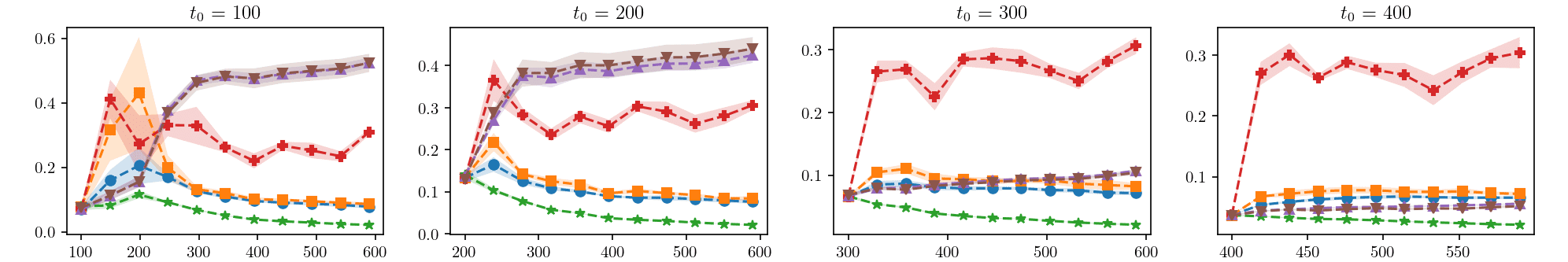
(a) Gowalla

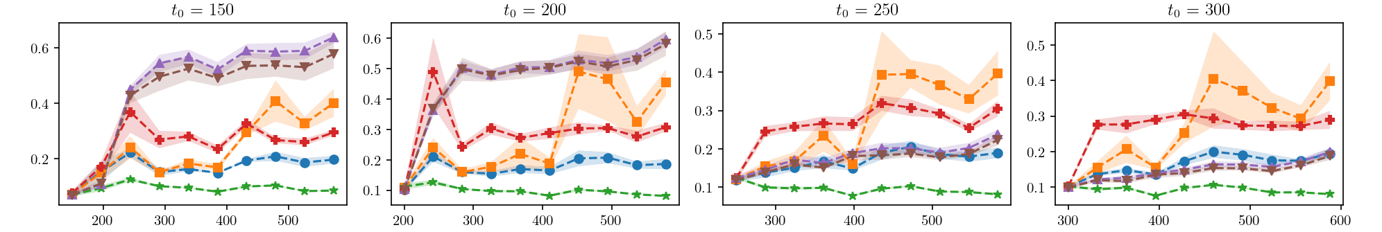
(b) Gowalla with deletion

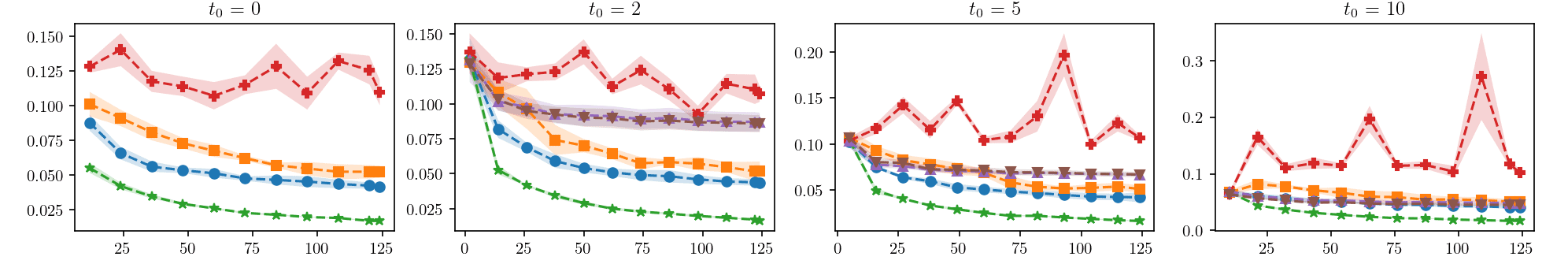
(c) New York taxi (over NY State)

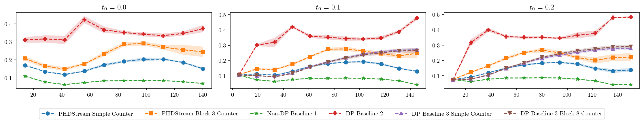
(d) Concentric circles with deletion

Figure 1: The progression of relative error in small range queries with time. All experiments are with privacy budget $\varepsilon=0.5$. Each subplot has a time horizon on the x-axis and corresponds to a particular value of $t_{0}$ (increasing from left to right).

5.1 Datasets

We conducted experiments on datasets with the location (latitude and longitude coordinates) of users collected over time. We analyzed the performance of our method on two real-world and three artificially constructed datasets.

Real-world Datasets: We use two real-world datasets: Gowalla (Cho et al., 2011) and NY Taxi (Donovan & Work, 2016). The Gowalla dataset contains location check-ins by a user on the social media app Gowalla. The NY Taxi dataset (Donovan & Work, 2016) contains the pickup and drop-off locations and times of Yellow Taxis in NY.

Simulated Datasets: Our first simulated dataset is derived from the Gowalla dataset. Motivated by the problem of releasing the location of active coronavirus infection cases, we consider each check-in as a report of infection and remove this check-in after $30$ days indicating that the reported individual has recovered. This creates a version of Gowalla with deletion. The second dataset contains points sampled on two concentric circles but the points first appear on one circle and then gradually move to the other circle. This creates a dataset where the underlying distribution changes dramatically. We also wanted to explore the performance of our algorithm based on the number of data points it observes in initialization and then at each batch. Thus for this dataset, we first fix a constant batch size for the experiment and then index time accordingly. Additionally, we keep initialization time $t_{0}$ as a value in $[0,1]$ denoting the proportion of total data the algorithm uses for initialization.

5.2 Initialization

Many real-world datasets such as Gowalla have a slow growth at the beginning of time. In practice, we can hold the processing of such streams until some time $t_{0}\in\mathbb{N}$, which we refer to as initialization time, until sufficient data has been collected. Thus for any input data stream $f\mathrel{\mathop{\mathchar 58\relax}}\Omega\times\mathbb{N}\to\mathbb{R}$ and initialization time $t_{0}\in\mathbb{N}$, we use a modified stream $\hat{f}\mathrel{\mathop{\mathchar 58\relax}}\Omega\times\mathbb{N}\to\mathbb{R}$ such that $\hat{f}(\cdot,t)=f(\cdot,t+t_{0}-1)$ for all $t\in\mathbb{N}$. We discuss the effects of initialization time $t_{0}$ on the algorithm performance in detail in Section 5.5

5.3 Baselines

Let $\varepsilon$ be our privacy budget. Consider the offline synthetic data generation algorithm as per (Zhang et al., 2016), which is to use $\operatorname{PrivTree}_{T}$ with privacy budget $\varepsilon/2$ to obtain a subtree $S$ of $T$, generate the synthetic count of each node $v\in\mathcal{L}(S)$ by adding Laplace noise with scale $2/\varepsilon$, and sample points in each node $v\in\mathcal{L}(S)$ equal to their synthetic count. Let us denote this algorithm as $\operatorname{PrivTree}_{T}+\operatorname{Counting}$. A basic approach to convert an offline algorithm to a streaming algorithm is to simply run independent instances of the algorithm at each time $t\in\mathbb{N}$. We use this idea to create the following three baselines and compare our algorithm with them.

Baseline 1) Offline PrivTree on stream: At any time $t\in\mathbb{N}$, we run an independent version of the offline $\operatorname{PrivTree}_{T}+\operatorname{Counting}$ on $f(\cdot,t)$, that is the stream data at time $t$. We want to emphasize that to be differentially private, this baseline requires a privacy parameter that scales with time $t$ and it does NOT satisfy differential privacy with the parameter $\varepsilon$. Thus we expect it to perform much better with an algorithm that is $\varepsilon$-DP. We still use this method as a baseline since, due to a lack of DP algorithms for streaming data, industry applications sometimes naively re-run DP algorithms as more data is collected. However, we show that PHDStream performs competitively close to this baseline.

Baseline 2) Offline PrivTree on differential stream Similar to Baseline 1, at any time $t\in\mathbb{N}$, we run an independent version of the offline $\operatorname{PrivTree}_{T}+\operatorname{Counting}$ algorithm, but with the input data $\nabla f(\cdot,t)$, that is the differential data observed at $t$. This baseline satisfies $\varepsilon$-DP. For a fair comparison, at time $t$, any previous output is discarded and the current synthetic data is scaled by the factor ${|f(\cdot,t)|}/{|\nabla f(\cdot,t)|}$.

Baseline 3) Initialization with PrivTree, followed by counting with counters: We first use the offline $\operatorname{PrivTree}_{T}+\operatorname{Counting}$ algorithm at only the initialization time $t_{0}$ and get a subtree $S$ of $T$ as selected by PrivTree. We then create a counter for all nodes $v\in\mathcal{L}(S)$ with privacy budget $\varepsilon$. At any time $t>t_{0}$, $S$ is not updated, and only the counter for each of the nodes in $\mathcal{L}(S)$ is updated using the differential stream $\nabla f(\cdot,t)$. This baseline also satisfies $\varepsilon$-DP. Note that this algorithm has twice the privacy budget for counting at each time $t>t_{0}$ as we do not update $S$. We only have results for this baseline if $t_{0}>0$. We show that PHDStream outperforms this baseline if the underlying density of points changes sufficiently with time.

5.4 Performance metric

We evaluate the performance of our algorithm against range counting queries, that count the number of points in a subset of the space $\Omega$. For $\Omega^{\prime}\subseteq\Omega$, the associated range counting query $q_{\Omega^{\prime}}$ over a function $h\mathrel{\mathop{\mathchar 58\relax}}\Omega\to\mathbb{R}$ is defined as $q_{\Omega^{\prime}}(h)\coloneqq\sum_{x\in\Omega^{\prime}}h(x)$. In our experiments, we use random rectangular subsets of $\Omega$ as the subregion for a query. Similar to (Zhang et al., 2016), we generate three sets of queries: $10,000$ small, $5000$ medium, and $1000$ large with area in $[0.01\%,0.1\%)$, $[0.1\%,1\%)$, and $[1\%,10\%)$ of the space $\Omega$ respectively. We use average relative error over a query set as our metric. At time $t$, given query set $Q$, the relative error of a synthetic stream $g\mathrel{\mathop{\mathchar 58\relax}}\Omega\times\mathbb{N}\to\mathbb{R}$ as compared to the input stream $f\mathrel{\mathop{\mathchar 58\relax}}\Omega\times\mathbb{N}\to\mathbb{R}$ is thus defined as,

$$r(Q,f,g,t)\coloneqq\frac{1}{|Q|}\sum_{q\in Q}\frac{\mathinner{\!\left\lvert q(f(\cdot,t))-q(g(\cdot,t))\right\rvert}}{\max{\left(q(f(\cdot,t)),0.001|f(\cdot,t)|\right)}}$$

where $0.001|f(\cdot,t)|$ or $1\%$ of $|f(\cdot,t)|$ is a small additive term to avoid division by $0$. We evaluate the metric for each query set at a regular time interval and report our findings.

5.5 Results

Our analysis indicates that PHDStream performs well across various datasets and hyper-parameter settings. We include some of the true and synthetic data images in Appendix H. Due to space constraints, we limit the discussion of the result to a particular setting in Figure 1 where we fix the privacy budget to $\varepsilon=1$, sensitivity to $2$, query set to small queries, and explore different values for initialization time $t_{0}$. For further discussion, refer to Appendices H and I.

PHDStream remains competitive to the challenging non-differentially private Baseline 1 and in almost all cases, it outperforms the differentially private Baseline 2. It also outperforms Baseline 3 if we initialize the algorithm sufficiently early. We discuss above mentioned observations together with the effect of various hyper-parameters below.

Initialization time: If the dataset grows without changing the underlying distribution too much, it seems redundant to update $T(t)$ with $\operatorname{PrivTree}_{T}$ at each time $t\in\mathbb{N}$. Moreover, when counting using fixed counters, we know that error in a counter grows with time so the performance of the overall algorithm should decrease with time. We observe the same for higher values of initialization time in Figure 1. Moreover, we see that Baseline 3, which uses PrivTree only once, outperforms PHDStream for such cases.

Counter type: In almost all cases, for the PHDStream algorithm, the Simple counter has better performance than the Block 8 counter. This can be explained by the fact that for these datasets, the majority of nodes had their counter activated only a few times in the entire algorithm. For example, when using the Gowalla dataset with $t_{0}=100$, on average, at least $90\%$ of total nodes created in the entire run of the algorithm had their counter activated less than $40$ times.

Sensitivity and batch size: We explore various values of sensitivity and batch size and the results are as expected - low sensitivity and large batch size improve the algorithm performance. For more details see Appendix I.

Appendix A $\operatorname{PrivTree}_{T}$ algorithm and its privacy

1:  Input: $F\in C(T)$, the privacy budget parameter $\varepsilon$, the threshold count for a node $\theta$.

2:  Output: A subset $S$ of the tree $T$.

3:  Set $\lambda\leftarrow\frac{2\beta-1}{\beta-1}\cdot\frac{2}{\varepsilon}$ and $\delta\leftarrow\lambda\ln{\beta}$.

4:  Initialize an empty tree $S$.

5:  $U\leftarrow\mathinner{\left\{root(T)\right\}}$; denotes a set of un-visited nodes.

6:  for $v\in U$ do

7:     Add $v$ to $S$.

8:     $U\leftarrow U\backslash\mathinner{\left\{v\right\}}$; mark $v$ visited.

9:     $b(v)\leftarrow F(v)-depth(v)\cdot\delta$; is a biased aggregate count of the node $v$.

10:     $b(v)\leftarrow\max\mathinner{\left\{b(v),\theta-\delta\right\}}$; to ensure that $b(v)$ is not too small.

11:     $\tilde{b}(v)\leftarrow b(v)+Lap(\lambda)$; noisy version of the biased count.

12:     if $(\tilde{b}(v)>\theta)$; noisy biased count is more than threshold then

13:        Add children of $v$ in $T$ to $U$.

14:     end if

15:  end for

Algorithm 5 $\operatorname{PrivTree}_{T}$

Proof of Theorem 3.1.

Similar to (Zhang et al., 2016) we define the following two functions:

$$\rho_{\lambda,\theta}(x)=\ln{\left(\frac{\mathbb{P}\left\{x+Lap(\lambda)>\theta\right\}}{\mathbb{P}\left\{x-1+Lap(\lambda)>\theta\right\}}\right)},$$ (7)

$$\rho^{\top}_{\lambda,\theta}(x)=\begin{cases}1/\lambda,&x<\theta+1,\\ \frac{1}{\lambda}\exp{\left(\frac{\theta+1-x}{\lambda}\right)},&otherwise.\end{cases}$$ (8)

It can be shown that $\rho_{\lambda,\theta}(x)\leq\rho^{\top}_{\lambda,\theta}(x)$ for any $x$.

Let us consider the neighbouring functions $F$ and $\tilde{F}$ such that $\mathinner{\!\left\lVert F-\tilde{F}\right\rVert}_{C(T)}=1$ and there exists $v_{*}\in V(T)$ such that $F(v_{*})\neq\tilde{F}(v_{*})$. Consider the output $S$, a subtree of $T$.

Case 1: $F(v_{*})>\tilde{F}(v_{*})$

Note that there will be exactly one leaf node in $S$ that differs in the count for the functions $F$ and $\tilde{F}$. Let $v_{1},v_{2},\dots,v_{k}$ be the path from the root to this leaf node. As per Algorithm 5, let us denote the calculated biased counts of any node $v\in S$ for the functions $F$ and $\tilde{F}$ as $b(v)$ and $\tilde{b}(v)$, respectively. Then, for any $v\in S$, we have the following relations,

$$\tilde{F}(v) =\begin{cases}F(v)-1,&v\in\mathinner{\left\{v_{1},v_{2},v_{3},\dots,v_{k}\right\}}\\ F(v),&otherwise,\end{cases}$$

$$\tilde{b}(v) =\begin{cases}b(v)-1,&v\in\mathinner{\left\{v_{1},v_{2},v_{3},\dots,v_{k}\right\}},b(v)>\theta-\delta,\\ b(v),&otherwise.\end{cases}$$

Let there exist an $m\in[k-1]$, s.t. $b(v_{m})\geq\theta-\delta+1$ and $b(v_{m+1})=\theta-\delta$. We then show that there is a difference in count by at least $\delta$ between parent and child for all $i\in[2,m]$

$$b(v_{i})=F(v_{i})-\delta\cdot depth(v)\leq F(v_{i-1})-\delta\cdot(depth(v_{i-1})+1)\leq b(v_{i-1})-\delta.$$

Thus we have,

$$\begin{cases}b(v_{i-1})\geq b(v_{i})+\delta\geq\theta+1,&i\in[2,m],\\ b(v_{i})=\theta-\delta,&otherwise.\end{cases}$$ (9)

Finally, we can show DP as follows,

$$\ln{\left(\frac{\mathbb{P}\left\{\mathcal{M}(F)=S\right\}}{\mathbb{P}\left\{\mathcal{M}(\tilde{F})=S\right\}}\right)}={} \sum_{i=1}^{k-1}\ln{\left(\frac{\mathbb{P}\left\{b(v_{i})+Lap(\lambda)>\theta\right\}}{\mathbb{P}\left\{\tilde{b}(v_{i})+Lap(\lambda)>\theta\right\}}\right)}+\ln{\left(\frac{\mathbb{P}\left\{b(v_{k})+Lap(\lambda)\leq\theta\right\}}{\mathbb{P}\left\{\tilde{b}(v_{k})+Lap(\lambda)\leq\theta\right\}}\right)}$$

$$={} \sum_{i=2}^{m}\ln{\left(\frac{\mathbb{P}\left\{b(v_{i})+Lap(\lambda)>\theta\right\}}{\mathbb{P}\left\{b(v_{i})-1+Lap(\lambda)>\theta\right\}}\right)}+\sum_{i=m+1}^{k-1}\ln{\left(\frac{\mathbb{P}\left\{b(v_{i})+Lap(\lambda)>\theta\right\}}{\mathbb{P}\left\{b(v_{i})+Lap(\lambda)>\theta\right\}}\right)}$$

$$+\ln{\left(\frac{\mathbb{P}\left\{b(v_{k})+Lap(\lambda)\leq\theta\right\}}{\mathbb{P}\left\{\tilde{b}(v_{k})+Lap(\lambda)\leq\theta\right\}}\right)}$$

$$[\text{Using the fact that }\ln{x}\leq 0\text{ for all }x\leq 1]$$

$$\leq{} \sum_{i=2}^{m}\ln{\left(\frac{\mathbb{P}\left\{b(v_{i})+Lap(\lambda)>\theta\right\}}{\mathbb{P}\left\{b(v_{i})-1+Lap(\lambda)>\theta\right\}}\right)}+0+0.$$

Using equations (7) and (8) we have,

$$\ln{\left(\frac{\mathbb{P}\left\{\mathcal{M}(F)=S\right\}}{\mathbb{P}\left\{\mathcal{M}(\tilde{F})=S\right\}}\right)}\leq{} \sum_{i=2}^{m}\rho_{\lambda,\theta}{(b(v_{i}))}\leq\sum_{i=2}^{m}\rho_{\lambda,\theta}^{\top}{(b(v_{i}))}=\rho_{\lambda,\theta}^{\top}{(b(v_{m}))}+\sum_{i=2}^{m-1}\rho_{\lambda,\theta}^{\top}{(b(v_{i}))}$$

$$={} \frac{1}{\lambda}+\sum_{i=2}^{m-1}\frac{1}{\lambda}\exp{\left(\frac{\theta+1-b(v_{i})}{\lambda}\right)}=\frac{1}{\lambda}+\sum_{i=1}^{m-2}\frac{1}{\lambda}\exp{\left(\frac{\theta+1-b(v_{m-i})}{\lambda}\right)}$$

$$[\text{Using equation \eqref{eq:countincrement} and }b(v_{m-1})\geq b(v_{m})+\delta\geq\theta+1]$$

$$\leq{} \frac{1}{\lambda}+\frac{1}{\lambda}\sum_{i=1}^{m-2}e^{-\delta/\lambda}\leq\frac{1}{\lambda}+\frac{1}{\lambda}\cdot\frac{1}{1-e^{-\delta/\lambda}}=\frac{1}{\lambda}\cdot\frac{2e^{\delta/\lambda}-1}{e^{\delta/\lambda}-1}=\varepsilon.$$

Case 2: $F(v_{*})<\tilde{F}(v_{*})$

Following the same notations as Case 1, for any $v\in S$, we have the following relations,

$$\tilde{F}(v) =\begin{cases}F(v)+1,&v\in\mathinner{\left\{v_{1},v_{2},v_{3},\dots,v_{k}\right\}},\\ F(v),&otherwise,\end{cases}$$

$$\tilde{b}(v) =\begin{cases}b(v)+1,&v\in\mathinner{\left\{v_{1},v_{2},v_{3},\dots,v_{k}\right\}},b(v)\geq\theta-\delta,\\ b(v),&otherwise.\end{cases}$$

Finally, we can show DP as follows,

$$\ln{\left(\frac{\mathbb{P}\left\{\mathcal{M}(F)=S\right\}}{\mathbb{P}\left\{\mathcal{M}(\tilde{F})=S\right\}}\right)}={} \sum_{i=1}^{k-1}\ln{\left(\frac{\mathbb{P}\left\{b(v_{i})+Lap(\lambda)>\theta\right\}}{\mathbb{P}\left\{\tilde{b}(v_{i})+Lap(\lambda)>\theta\right\}}\right)}+\ln{\left(\frac{\mathbb{P}\left\{b(v_{k})+Lap(\lambda)\leq\theta\right\}}{\mathbb{P}\left\{\tilde{b}(v_{k})+Lap(\lambda)\leq\theta\right\}}\right)}$$

$$[\text{Since }\ln{x}\leq 0\text{ for all }x\leq 1]$$

$$\leq 0+\ln{\left(\frac{\mathbb{P}\left\{b(v_{k})+Lap(\lambda)\leq\theta\right\}}{\mathbb{P}\left\{\tilde{b}(v_{k})+1+Lap(\lambda)\leq\theta\right\}}\right)}\leq\varepsilon.$$

Hence the algorithm is $\varepsilon$-differentially private.

∎

Appendix B Poof of privacy of PHDStream

Proof of Theorem 3.2.

It suffices to show that PHDStreamTree is $\varepsilon$-differentially private, since PHDStream is doing a post-processing on its output which is independent of the input data stream. Let $f$ and $\tilde{f}$ be neighboring data streams such that $\mathinner{\!\left\lVert f-\tilde{f}\right\rVert}_{\nabla}=1$. Let $F$ and $\tilde{F}$ be the corresponding streams on the vertices of $T$ respectively. Since $f$ and $\tilde{f}$ are neighbors, there exists $\tau\in\mathbb{N}$ such that $\mathinner{\!\left\lVert\nabla F(\cdot,\tau)-\nabla\tilde{F}(\cdot,\tau)\right\rVert}_{C(T)}=1$. Note that, at any time $t$, PHDStreamTree only depends on $\nabla F_{t}$ from the input data stream. Hence for the differential privacy over the entire stream, it is sufficient to show that the processing at time $\tau$ is differentially private. Note that both $\operatorname{PrivTree}_{T}$ and the calculation of $d(\cdot,t)$ satisfy $\varepsilon/2$-differential privacy by Theorem 3.1 and by the Laplace Mechanism, respectively. Hence their combination, that is PHDStreamTree at time $\tau$, satisfies $\varepsilon$-differential privacy. At any $t\neq\tau$, $\nabla F(v,t)=\nabla\tilde{F}(v,t)$ for all $v\in T$. Hence PHDStreamTree satisfies $\varepsilon$-differential privacy for the entire input stream $F$. ∎

Appendix C Optimizing the algorithm

In Algorithm 1, at any time $t$, we have to perform computations for every node $v\in T$. Since $T$ can be a tree with large depth and the number of nodes is exponential with respect to depth, the memory and time complexity of PHDStreamTree, as described in Algorithm 1 is also exponential in depth of the tree $T$. Note however that we do not need the complete tree $T$, and can limit all computations to the subtree $T(t)$ as selected by PrivTree at time $t$. Based on this idea, we propose a version of PHDStream in Algorithm 6 which is storage and runtime efficient.

1:  Input: Input data stream $f\mathrel{\mathop{\mathchar 58\relax}}\Omega\times\mathbb{N}\to\mathbb{R}$, a fixed and known tree $T$, the privacy budget parameter $\varepsilon$, the threshold count for a node $\theta$.

2:  Output: A synthetic data stream $g\mathrel{\mathop{\mathchar 58\relax}}\Omega\times\mathbb{N}\to\mathbb{R}$.

3:  Set $\lambda\leftarrow\frac{2\beta-1}{\beta-1}\cdot\frac{2}{\varepsilon}$ and $\delta\leftarrow\lambda\ln{\beta}$.

4:  Initialize $C_{a}$, $C_{n}$, and $C_{d}$ and make them accessible to Algorithm 7.

5:  for every time $t\in\mathbb{N}$ do

6:     Set $T(t)$ as the output of Algorithm 7 with parameters $(\nabla f(\cdot,t),\delta,\theta,\lambda,\varepsilon/2)$.

7:     Calculate $G(v)\leftarrow C_{a}(v)+C_{n}(v)+C_{d}(v)$ for all $v\in leaves(T(t))$.

8:     Convert $G$ to $g(\cdot,t)$ as per equation 5.

9:  end for

Algorithm 6 Compute efficient PHDStream

1:  Input: Count of points in $\Omega$ as $h\mathrel{\mathop{\mathchar 58\relax}}\Omega\to\mathbb{R}$, parameters related to privacy $\delta,\theta,\lambda,\varepsilon^{\prime}$.

2:  Output: A subtree $T^{*}$ of $T$.

3:  Initialize an empty subtree $T^{*}$ of $T$.

4:  Initialize a queue $Q$ of un-visited nodes.

5:  Push $root(T)$ to $Q$.

6:  Initialize an empty stack $S$.

7:  while $Q$ is not empty do

8:     Pop $v$ from $Q$.

9:     Add $v$ to the subtree $T^{*}$.

10:     Find $H(v)$ using $h$ as per equation 4.

11:     To enforce ancestor consistency, update$C_{a}(v)\leftarrow\frac{1}{\beta}\cdot\left(C_{a}(parent(v))+C_{n}(parent(v))\right)$.

12:     Set $s(v)\leftarrow C_{a}(v)+C_{n}(v)+C_{d}(v)$

13:     Set $b(v)\leftarrow\left(s(v)+H(v)-depth(v)\cdot\delta\right)$; as biased count of the node $v$.

14:     $b(v)\leftarrow\max\mathinner{\left\{b(v),\theta-\delta\right\}}$; to ensure that $b(v)$ is not too small.

15:     $\hat{b}(v)\leftarrow b(v)+Lap(\lambda)$; noisy version of the biased count.

16:     if $\left(\hat{b}(v)>\theta\right)$ and $children(v)$ is not empty in $T$ then

17:        Push $w$ to $Q$ for all $w\in children(v)$ in $T$.

18:        Push $v$ to $S$.

19:     else

20:        Update $C_{n}(v)\leftarrow C_{n}(v)+H(v)+Lap(2/\varepsilon^{\prime})$ .

21:     end if

22:  end while

23:  while $S$ is not empty do

24:     Pop $v$ from $S$.

25:     To enforce descendant consistency, update$C_{d}(v)\leftarrow\sum_{w\in children(v)}\left(C_{d}(w)+C_{n}(w)\right)$.

26:  end while

Algorithm 7 Modified $\operatorname{PrivTree}_{T}$ subroutine

Note that in Algorithm 1, at any time $t\in\mathbb{N}$, we find the differential synthetic count of any node $v$ as $d(v,t)$ only if $v$ is a leaf in $T(t)$. To maintain the consistency, as given by equation 6, this count gets pushed up to ancestors or spreads down to the descendants by the consistency extension operator $Ext_{T}$. A key challenge in efficiently enforcing consistency is that we do not want to process nodes that are not present in $T(t)$. Since the operator $Ext_{T}$ is linear if we have the total differential synthetic count of all nodes $v$ till time $t$, that is $\sum_{t^{\prime}\leq t}d(v,t^{\prime})$, we can find the count of any node resulting after consistency extension. We track this count in a function $C_{n}\mathrel{\mathop{\mathchar 58\relax}}V(T)\to\mathbb{R}$ such that at any time $t$, $C_{n}(v)$ represents the total differential synthetic count of node $v$ for times $t^{\prime}\leq t$ when $v\in leaves(T(t^{\prime}))$. We update the value $C_{n}(v)$ for any node $v\in leaves(T(t))$ as,

$$C_{n}(v)\leftarrow C_{n}(v)+\left(\nabla F(v)+Lap(2/\varepsilon)\right).$$

Furthermore, to efficiently enforce consistency, we introduce $C_{a}$ and $C_{d}$ mappings $V(T)\to\mathbb{R}$. At any time $t$, $C_{a}(v)$ and $C_{d}(v)$ denote the count a node $v$ has received at time $t$ when enforcing consistency from its ancestors and descendants, respectively. Consistency due to counts being passed down from ancestors can be enforced with the equation

$$C_{a}(v)=\frac{1}{\beta}\cdot\left(C_{a}(parent(v))+C_{n}(parent(v))\right).$$ (10)

Consistency due to counts being pushed up from descendants can be enforced with the equation

$$C_{d}(v)=\sum_{w\in children(v)}\left(C_{d}(w)+C_{n}(w)\right).$$ (11)

We assume that $C_{a}(v)=C_{n}(v)=C_{d}(v)=0$ for all $v\in V(T)$ at the beginning of Algorithm 6. With the help of these functions, the synthetic count of any node $v\in T(t)$ can be calculated as $s(v)=C_{a}(v)+C_{n}(v)+C_{d}(v)$.

Algorithm 7 is a modified version of PrivTree Algorithm 5. We use it as a subroutine of Algorithm 6, where at time $t$ it is responsible for creating the subtree $T(t)$ and updating the values of the functions $C_{a}$, $C_{n}$, and $C_{d}$.

The algorithm uses two standard data structures called Stack and Queue which are ordered sets where the order is based on the time at which the elements are inserted. We interact with the data structures using two operations Push and Pop. Push is used to insert an element, whereas pop is used to remove an element. The key difference between a Queue and a Stack is that the operation pop on a Queue returns the element inserted earliest but on a Stack returns the element inserted latest. Thus Queue and Stack follow the FIFO (first-in, first-out) and LIFO (last-in, first-out) strategy, respectively.

C.1 Privacy of compute-efficient PHDStream

At any time $t\in\mathbb{N}$, the key difference of Algorithm 6 (compute efficient PHDStream) from Algorithm 2 (PHDStream) is that (1) it does not compute $\nabla F(v,t)$ for any node $v\in T\setminus T(t)$, and (2) it does not use the consistency operator $Ext_{T}$ and instead relies on the mappings $C_{a}$, $C_{n}$, and $C_{d}$. Note that none of these changes affect the constructed tree $T(t)$ and the output stream $g(\cdot,t)$. Since both algorithms are equivalent in their output and Algorithm 2 is $\varepsilon$-differentially private, we conclude that Algorithm 6 is also $\varepsilon$-differentially private.

Appendix D Counters

We provide the algorithms for Simple, Block, and Binary Tree counter in Algorithms 8, 9, and 10 respectively. As proved in (Dwork et al., 2010; Chan et al., 2010) for a fixed failure probability $\delta$, ignoring the constants, the accuracy $\alpha$ at time $t$ for the counters Simple, Block, and Binary Tree is $\mathcal{O}\left(\sqrt{t}\right)$, $\mathcal{O}\left(t^{1/4}\right)$, and $\mathcal{O}\left(\left(\ln{t}\right)^{3/2}\right)$ respectively. Hence the error in the estimated value in counters grows with time $t$. The result also suggests that for large time horizons, the Binary Tree algorithm is best to be used as a counter. However, for small values of time $t$, the bounds suggest that Simple and Block counters are perhaps more effective. Note that the optimal size of the block in a Block Counter is suggested to be $\lfloor\sqrt{t}\rfloor$ where $t$ is the time horizon for the stream. However, in our method, we do not know in advance the time horizon for the stream that is input for a particular counter. After multiple experiments, we found that a Block counter with size 8 was most effective for our method PHDStream for the datasets in our experiments. Figure 2 shows an experiment comparing these counters. We observe that the Binary Tree algorithm should be avoided on streams of small time horizons, say $T<100$. Block counter appears to have lower errors for $T>30$. However, due to the large growth in error within a block, for $T<30$ it is unclear if the Block counter is better than the Simple counter.

1:  Input: Input stream $f\mathrel{\mathop{\mathchar 58\relax}}\mathbb{N}\to\mathbb{R}$, privacy budget $\varepsilon$

2:  Output: Output stream $g\mathrel{\mathop{\mathchar 58\relax}}\mathbb{N}\to\mathbb{R}$

3:  Assume $g(0)\leftarrow 0$

4:  Set $g(t)\leftarrow g(t-1)+f(t)+Lap(\frac{1}{\varepsilon})$ for all $t\in\mathbb{N}$

Algorithm 8 Simple counter

1:  Input: Input stream $f\mathrel{\mathop{\mathchar 58\relax}}\mathbb{N}\to\mathbb{R}$, privacy budget $\varepsilon$, block size $B$

2:  Output: Output stream $g\mathrel{\mathop{\mathchar 58\relax}}\mathbb{N}\to\mathbb{R}$

3:  $\alpha\leftarrow 0,\beta\leftarrow 0,\beta_{lastblock}\leftarrow 0$

4:  for $t=1,2,\dots$ do

5:     $\beta\leftarrow\beta+f(t)$

6:     if $t=k\cdot B$, for some $k\in\mathbb{N}$ then

7:        $\alpha\leftarrow 0$, $\beta\leftarrow\beta+Lap(\frac{2}{\varepsilon})$

8:        $\beta_{lastblock}\leftarrow\beta$

9:     else

10:        $\alpha\leftarrow\alpha+f(t)+Lap(\frac{2}{\varepsilon})$

11:     end if

12:     $g(t)\leftarrow\beta_{lastblock}+\alpha$

13:  end for

Algorithm 9 Block counter with block size $B$

1:  Input: Input stream $f\mathrel{\mathop{\mathchar 58\relax}}\mathbb{N}\to\mathbb{R}$, privacy budget $\varepsilon$, time horizon $T$

2:  Output: Output stream $g\mathrel{\mathop{\mathchar 58\relax}}\mathbb{N}\to\mathbb{R}$

3:  Initialize $\alpha_{i},\hat{\alpha}_{i}\leftarrow 0$ for all $i\in\mathbb{N}$

4:  for $t=1,2,\dots$ do

5:     Let $b_{n}\dots b_{1}b_{0}$ be the $(n+1)$-bit binary representation of $t$, i.e., $t=\sum_{i=0}^{n}b_{i}2^{i}$

6:     $j\leftarrow\min{\mathinner{\left\{i\mathrel{\mathop{\mathchar 58\relax}}b_{i}\neq 0\right\}}}$

7:     $\alpha_{j}\leftarrow\left(\sum_{i=0}^{j-1}\alpha_{i}\right)+f(t)$

8:     $\hat{\alpha}_{j}\leftarrow\alpha_{j}+Lap(\frac{\log_{2}{T}}{\varepsilon})$

9:     $\alpha_{i},\hat{\alpha}_{i}\leftarrow 0$ for all $i<j$

10:     $g(t)\leftarrow\sum_{i=0}^{n}\hat{\alpha}_{i}\cdot({\mathds{1}}_{b_{i}=1})$

11:  end for

Algorithm 10 Binary Tree counter

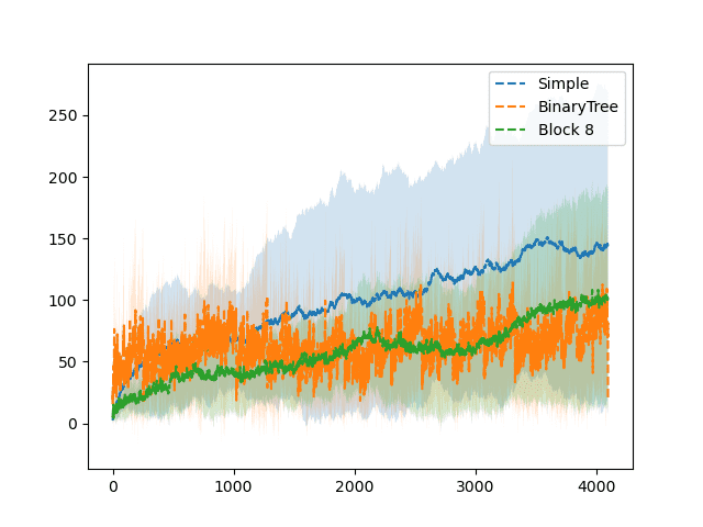
(a) Long time horizon of $2^{12}=4096$

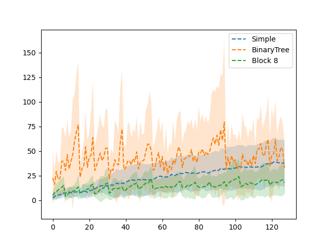
(b) Short time horizon of $2^{7}=128$

Figure 2: Comparing Simple, Block with size 8, and Binary Tree counters with privacy budget $\varepsilon=0.5$. The true data is a random bit stream of 0s and 1s. On the y-axis, we have the absolute error in the value of the counter at any time averaged over 10 independent runs of the counter algorithm.

Appendix E Privacy of selective counting

Proof.

Let us denote Algorithm 4 as $\mathcal{A}$. Let $f$ and $\tilde{f}$ be neighboring data streams with $\mathinner{\!\left\lVert f-\tilde{f}\right\rVert}=1$. Without loss of generality, there exists $\tau\in\mathbb{N}$ such that $f(\tau)=\tilde{f}(\tau)+1$. Let $g$ be the output stream we are interested in. Let ${\left.\kern-1.2pt{f}\right|_{[t]}}$ denote a restriction of the stream $f$ until time $t$ for any $t\in\mathbb{N}$.

Since the input streams are identical till time $\tau$, we have,

$$\mathbb{P}\left\{\mathcal{A}\left({\left.\kern-1.2pt{f}\right|_{[\tau-1]}}\right)={\left.\kern-1.2pt{g}\right|_{[\tau-1]}}\right\} =\mathbb{P}\left\{\mathcal{A}\left({\left.\kern-1.2pt{\tilde{f}}\right|_{[\tau-1]}}\right)={\left.\kern-1.2pt{g}\right|_{[\tau-1]}}\right\}$$

At time $\tau$, let $g(\tau)=(l_{\tau},m_{\tau})$. Since $\mathcal{M}$ is $\varepsilon_{M}$-DP, we have,

$$\mathbb{P}\left\{\mathcal{M}\left({\left.\kern-1.2pt{f}\right|_{[\tau]}},{\left.\kern-1.2pt{g}\right|_{[\tau-1]}}\right)=l_{\tau}\right\} \leq e^{\varepsilon_{M}}\cdot\mathbb{P}\left\{\mathcal{M}\left({\left.\kern-1.2pt{\tilde{f}}\right|_{[\tau]}},{\left.\kern-1.2pt{g}\right|_{[\tau-1]}}\right)=l_{\tau}\right\}.$$

Moreover, since $\mathcal{M}_{l_{\tau}}$ is $\varepsilon_{C}$-DP,

$$\mathbb{P}\left\{\mathcal{C}_{l_{\tau}}\left({\left.\kern-1.2pt{f}\right|_{J_{l_{t}}}}\right)=m_{\tau}\right\} \leq e^{\varepsilon_{C}}\cdot\mathbb{P}\left\{\mathcal{C}_{l_{\tau}}\left({\left.\kern-1.2pt{\tilde{f}}\right|_{J_{l_{t}}}}\right)=m_{\tau}\right\}.$$

Combining the above two we have,

$$\mathbb{P}\left\{\mathcal{A}\left({\left.\kern-1.2pt{f}\right|_{[\tau]}}\right)=g(\tau)\right\} =\mathbb{P}\left\{\mathcal{A}\left({\left.\kern-1.2pt{f}\right|_{[\tau-1]}}\right)={\left.\kern-1.2pt{g}\right|_{[\tau-1]}}\right\}\cdot\mathbb{P}\left\{\mathcal{M}\left({\left.\kern-1.2pt{f}\right|_{[\tau]}},{\left.\kern-1.2pt{g}\right|_{[\tau-1]}}\right)=l_{\tau}\right\}\cdot\mathbb{P}\left\{\mathcal{C}_{l_{\tau}}\left({\left.\kern-1.2pt{f}\right|_{J_{l_{t}}}}\right)=m_{\tau}\right\}$$

$$\leq\mathbb{P}\left\{\mathcal{A}\left({\left.\kern-1.2pt{\tilde{f}}\right|_{[\tau-1]}}\right)={\left.\kern-1.2pt{g}\right|_{[\tau-1]}}\right\}\cdot e^{\varepsilon_{M}}\mathbb{P}\left\{\mathcal{M}\left({\left.\kern-1.2pt{\tilde{f}}\right|_{[\tau]}},{\left.\kern-1.2pt{g}\right|_{[\tau-1]}}\right)=l_{\tau}\right\}\cdot e^{\varepsilon_{C}}\mathbb{P}\left\{\mathcal{C}_{l_{\tau}}\left({\left.\kern-1.2pt{\tilde{f}}\right|_{J_{l_{t}}}}\right)=m_{\tau}\right\}$$

$$=e^{(\varepsilon_{M}+\varepsilon_{C})}\cdot\mathbb{P}\left\{\mathcal{A}\left({\left.\kern-1.2pt{\tilde{f}}\right|_{[\tau]}}\right)=g(\tau)\right\}.$$

At any time $t>\tau$, since the input data streams are identical, we have,

$$\mathbb{P}\left\{\mathcal{A}\left({\left.\kern-1.2pt{f}\right|_{[t]}}\right)={\left.\kern-1.2pt{g}\right|_{[t]}}\right\} \leq e^{(\varepsilon_{M}+\varepsilon_{C})}\cdot\mathbb{P}\left\{\mathcal{A}\left({\left.\kern-1.2pt{\tilde{f}}\right|_{[t]}}\right)={\left.\kern-1.2pt{g}\right|_{[t]}}\right\}.$$

Hence, algorithm $\mathcal{A}$ is $(\varepsilon_{M}+\varepsilon_{C})$-DP. ∎

Appendix F Other experiment details

All the experiments were performed on a personal device with 8 cores of 3.60GHz 11th Generation Intel Core i7 processor and 32 GB RAM. Given the compute restriction, for any of the datasets mentioned below, we limit the total number of data points across the entire time horizon to the (fairly large) order of $10^{5}$. Moreover, the maximum time horizon for a stream we have is $300$ for Gowalla Dataset. We consider it to be sufficient to show the applicability of our algorithm for various use cases.

We implement all algorithms in Python and in order to use the natural geometry of the data domain we rely on the spatial computing libraries GeoPandas (Jordahl et al., 2020), Shapely (Gillies et al., 2023), NetworkX (Hagberg et al., 2008), and OSMnx (Boeing, 2017). These libraries allow us to efficiently perform operations such as loading the geometry of a particular known region, filtering points in a geometry, and sampling/interpolating points in a geometry.

Appendix G Datasets and Geometry

G.1 Datasets

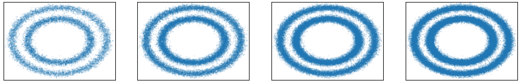
(a) Without deletion, where density on both circles grow with time

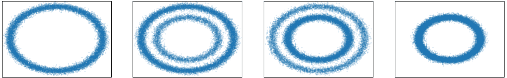
(b) With deletion, where the density gradually changes from predominantly on the outer circle to the inner circle

Figure 3: Scatter plot for the simulated datasets of two concentric circles showing the resulting location of users at four different times steps progressing from left to right

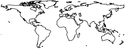
(a) Gowalla

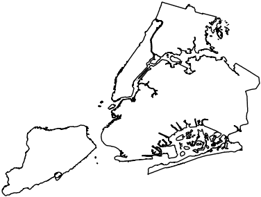
(b) New York taxi (over NY State)

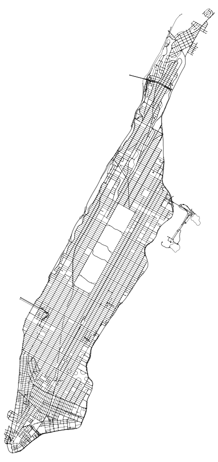
(c) New York Taxi (over road network of Manhattan)

Figure 4: Geometry used for datasets

Gowalla: The Gowalla dataset (Cho et al., 2011) contains location check-ins by a user along with their user id and time on the social media app Gowalla. For this dataset, we use the natural land geometry of Earth except for the continent Antarctica (see Figure 4(a) in Appendix G). The size of the dataset after restriction to the geometry is about $6.2$ million. We limit the total number of data points to about $200$ thousand and follow a daily release frequency based on the available timestamps.

Gowalla with deletion: To evaluate our method on a dataset with deletion that represents a real-world scenario, we create a version of the Gowalla dataset with deletion. Motivated by the problem of releasing the location of active coronavirus infection cases, we consider each check-in as a report of infection and remove this check-in after $30$ days indicating that the reported individual has recovered.

NY taxi: The NY Taxi dataset (Donovan & Work, 2016) contains the pickup and drop-off locations and times of Yellow Taxis in New York. For this dataset, we only use data from January $2013$ which already has more than $14$ million data points. We keep the release frequency to $6$ hours and restrict total data points to about $10^{5}$ sampling proportional to the number of data points at each time within the overall time horizon. We consider two different underlying geometries for this dataset. The first is the natural land geometry of the NY State as a collection of multiple polygons. The second is the road network of Manhattan Island as a collection of multiple curves. We include a figure of these geometries in Figure 4(b) and Figure 4(c) respectively of Appendix G. The second geometry is motivated by the fact that the majority of taxi pickup locations are on Manhattan Island and also on its road network.

Concentric circles: We also conducted experiments on an artificial dataset of points located on two concentric circles. As shown in Figure 3, we have two different scenarios of this dataset: (a) where both circles grow over time and (b) where the points first appear in one circle and then gradually move to the other circle. Scenario (b) helps us analyze the performance of our algorithm on a dataset where (unlike Gowalla and NY Taxi datasets) the underlying distribution changes dramatically. We also wanted to explore the performance of our algorithm based on the number of data points it observes in initialization and then at each batch. Thus for this dataset, we first fix a constant batch size for the experiment and then index time accordingly. Additionally, we keep initialization time $t_{0}$ as a value in $[0,1]$ denoting the proportion of total data the algorithm uses for initialization. We explore various parameters on these artificial datasets such as batch size, initialization data ratio, and sensitivity.

G.2 Initialization Time

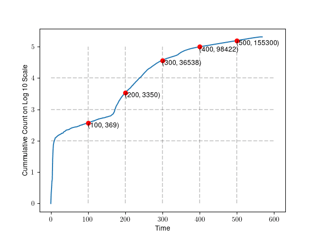
(a) Gowalla

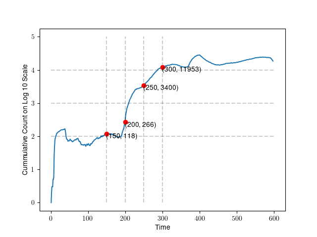
(b) Gowalla with deletion

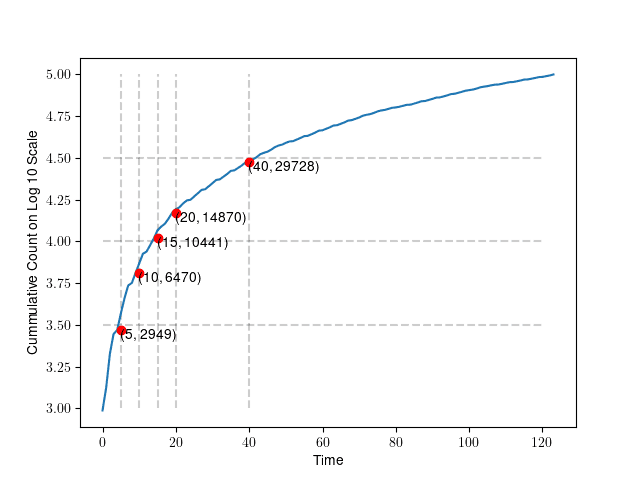
(c) NY Taxi

Figure 5: Cummulative count as time progresses for Gowalla and NY Taxi Dataset. The plot illustrates our motivation for the choice of initialization time.

In Figure 5, we show how the total number of data points change with time for the Gowalla and NY Taxi Datasets. For our algorithm to work best, we recommend having points in the order of at least $100$ at each time of the differential stream. Hence, based on the cumulative count observed in Figure 5 we select minimum $t_{0}=100$ for Gowalla, $t_{0}=150$ for Gowalla with deletion, and $t_{0}=0$ for NY Taxi datasets.

Appendix H Synthetic data scatter plots

In this section, we present a visualization of the synthetic data generated by our algorithm PHDStream with the Simple counter. We present scatter plots comparing the private input data with the generated synthetic data in Figures 6, 7, 8, and 9 for the datasets Gowalla, NY Taxi, and Concentric Circles with deletion respectively. Due to space limitations, we only show the datasets a few times, with time increasing from left to right. In each of the figures mentioned above, the first row corresponds to the private input data and is labeled ”True”. In each subplot, we plot the coordinates present at that particular time after accounting for all additions and deletions so far. Each of the following rows corresponds to one run of the PHDStream algorithm with the Simple counter and for a particular privacy budget $\varepsilon$ as labeled on the row. In each subplot, we use black dashed lines to create a partition of the domain corresponding to the leaves of the current subtree as generated by $\operatorname{PrivTree}_{T}$. For comparison, we overlay the partition created by the algorithm with $\varepsilon=0.5$ on the true data plot as well.

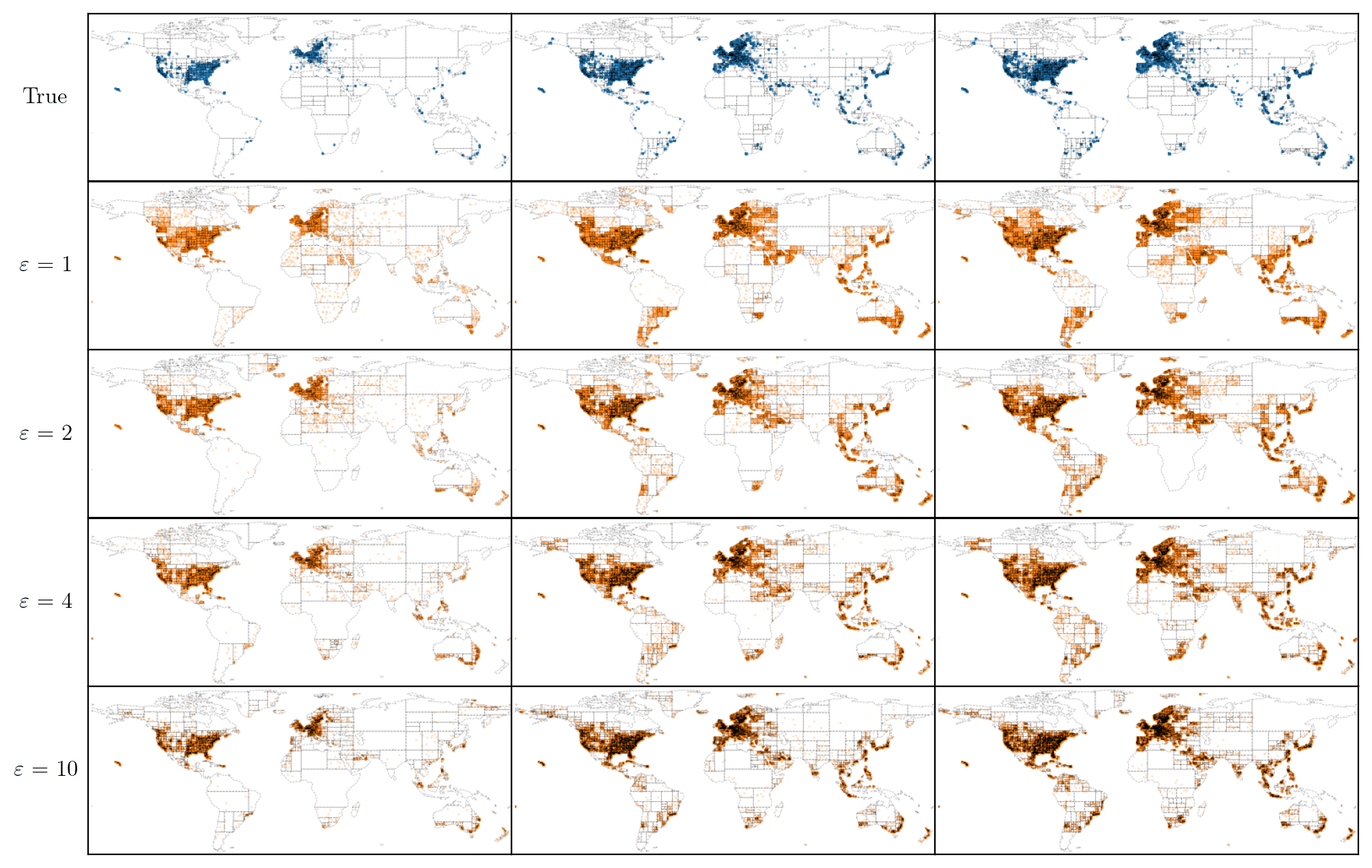
Figure 6: Scatter plot of True and Synthetic data (generated by PHDStream) over the Gowalla dataset for initialization time index $t_{0}=100$

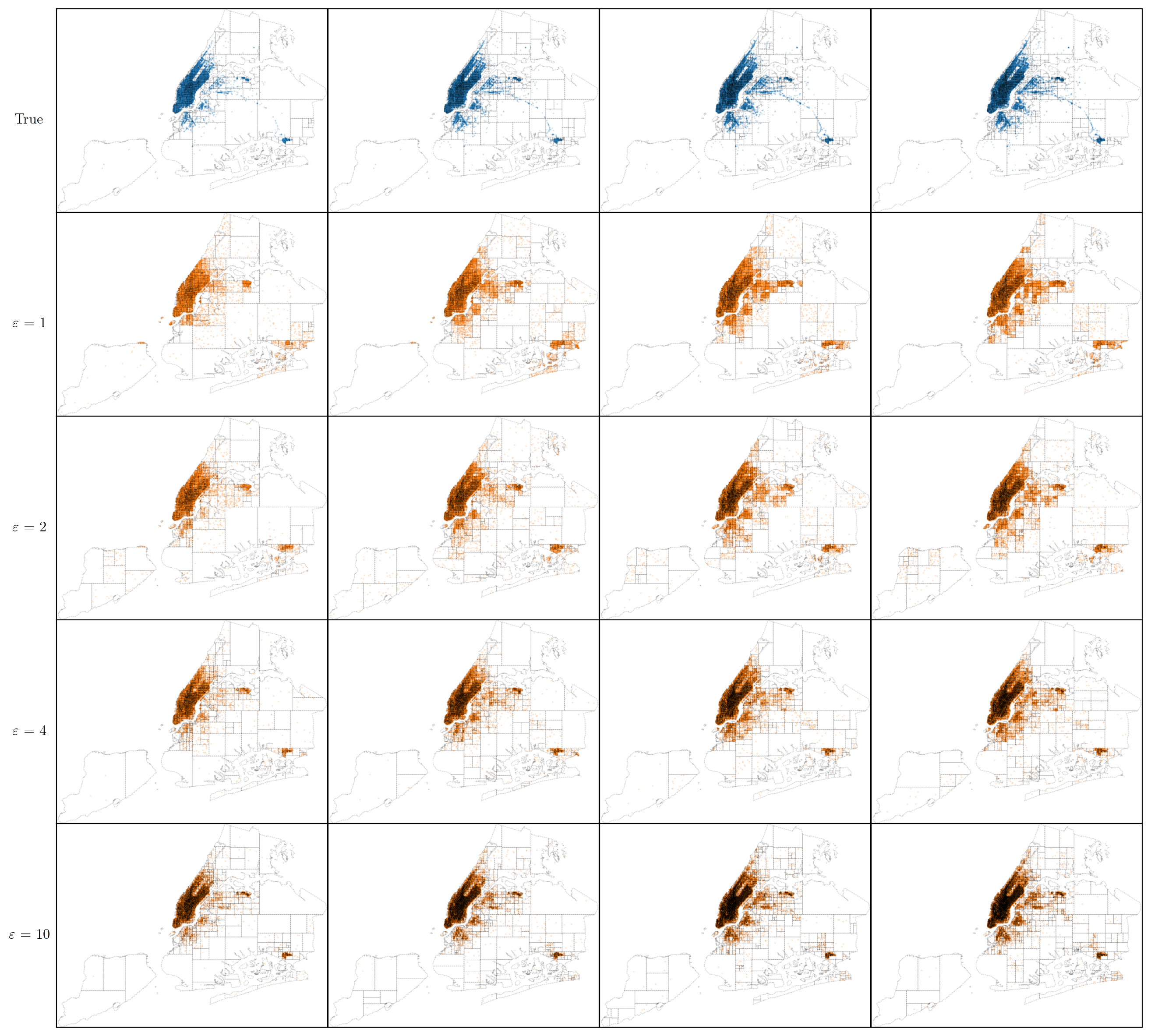
Figure 7: Scatter plot of True and Synthetic data (generated by PHDStream) over the New York dataset over NY State for initialization time index $t_{0}=2$

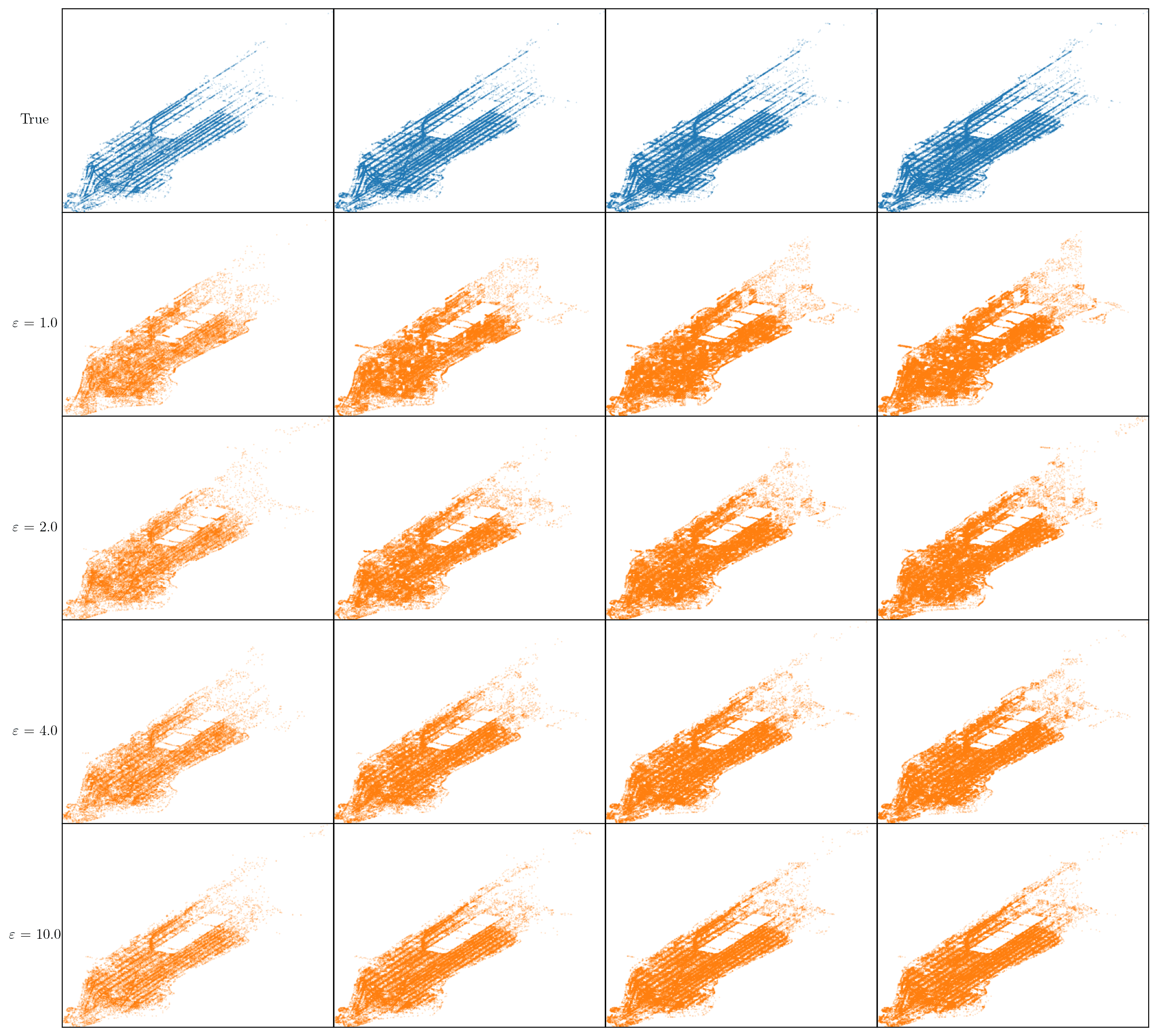
Figure 8: Scatter plot of True and Synthetic data (generated by PHDStream) over the New York dataset over road network of Manhattan for initialization time index $t_{0}=2$

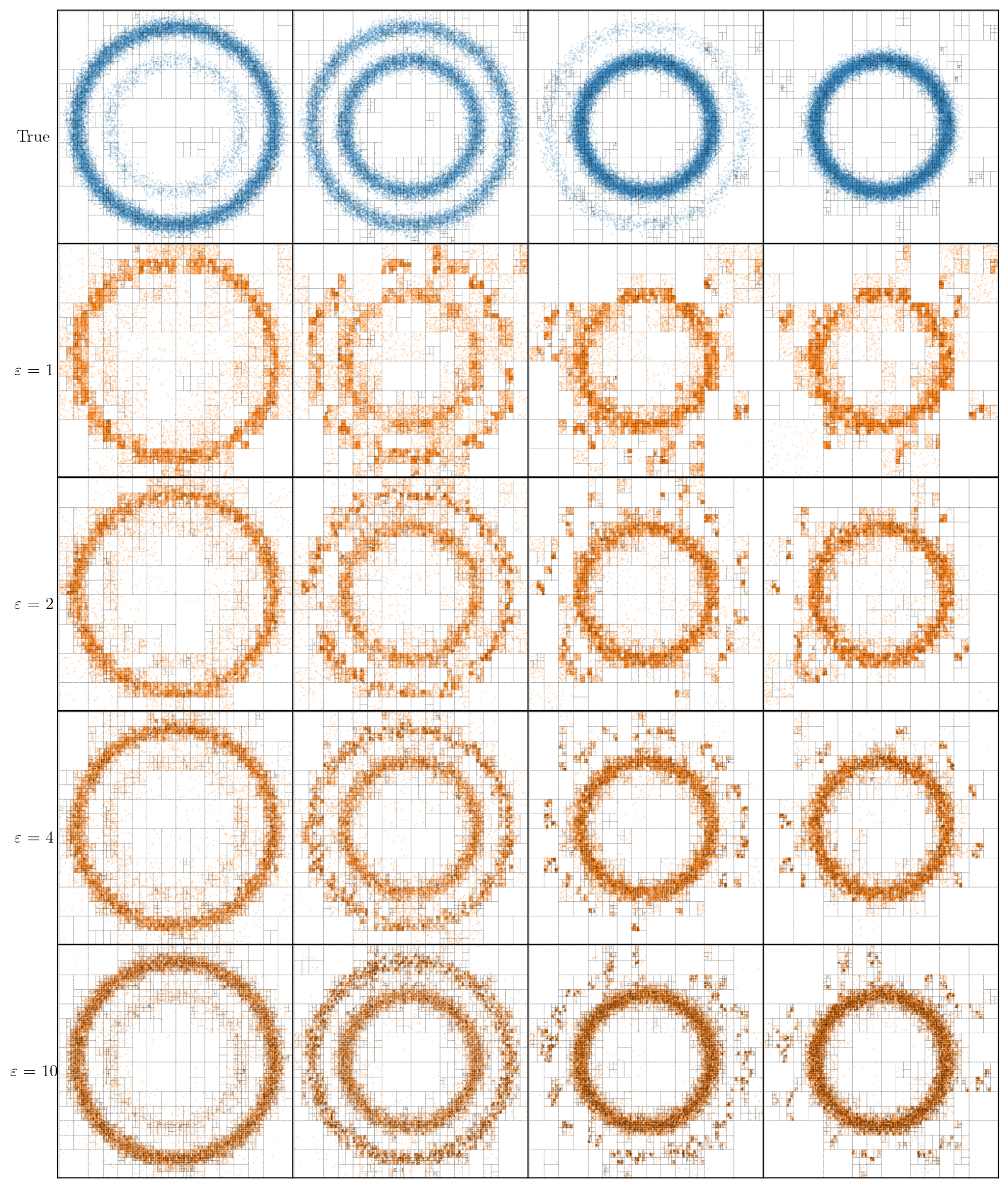
Figure 9: Scatter plot of True and Synthetic data (generated by PHDStream) over the Concentric circles with deletion dataset for initialization data ratio $t_{0}=0.1$, constant batch size $500$

Appendix I More Results

Figures 10, 11, 12, 13, 14, and 15 show a comparison of performances on different datasets for small-range queries. Each subplot has a time horizon on the x-axis and corresponds to a particular value of privacy budget $\varepsilon$ (increasing from left to right) and initialization time $t_{0}$ (increasing from top to bottom). We do not show PHDStream with Block counter and Baseline 2 in these figures as they both have very large errors in some cases and that distorts the scale of the figures. We also show some results on medium and large scale range queries (as described in Section 5.4) for the dataset Gowalla in Figures 16,  17 and for the dataset Gowalla with deletion in Figures 18,  19 respectively.

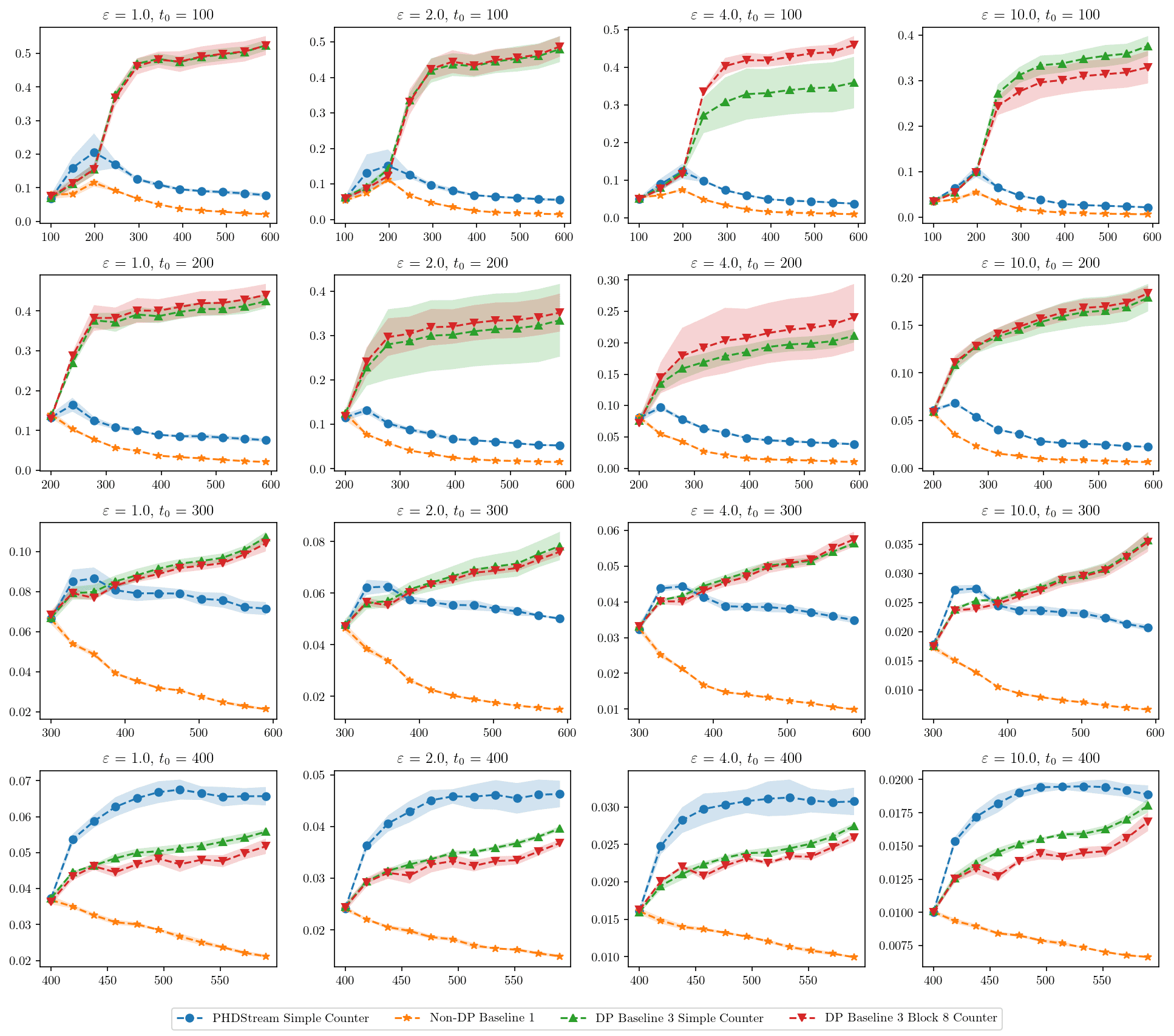
Figure 10: Query error for PHDStream over the dataset Gowalla and small range queries.

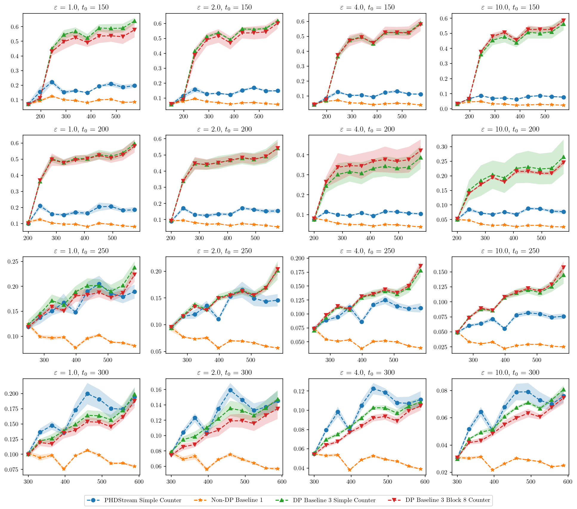
Figure 11: Query error for PHDStream over the dataset Gowalla with deletion and small range queries.

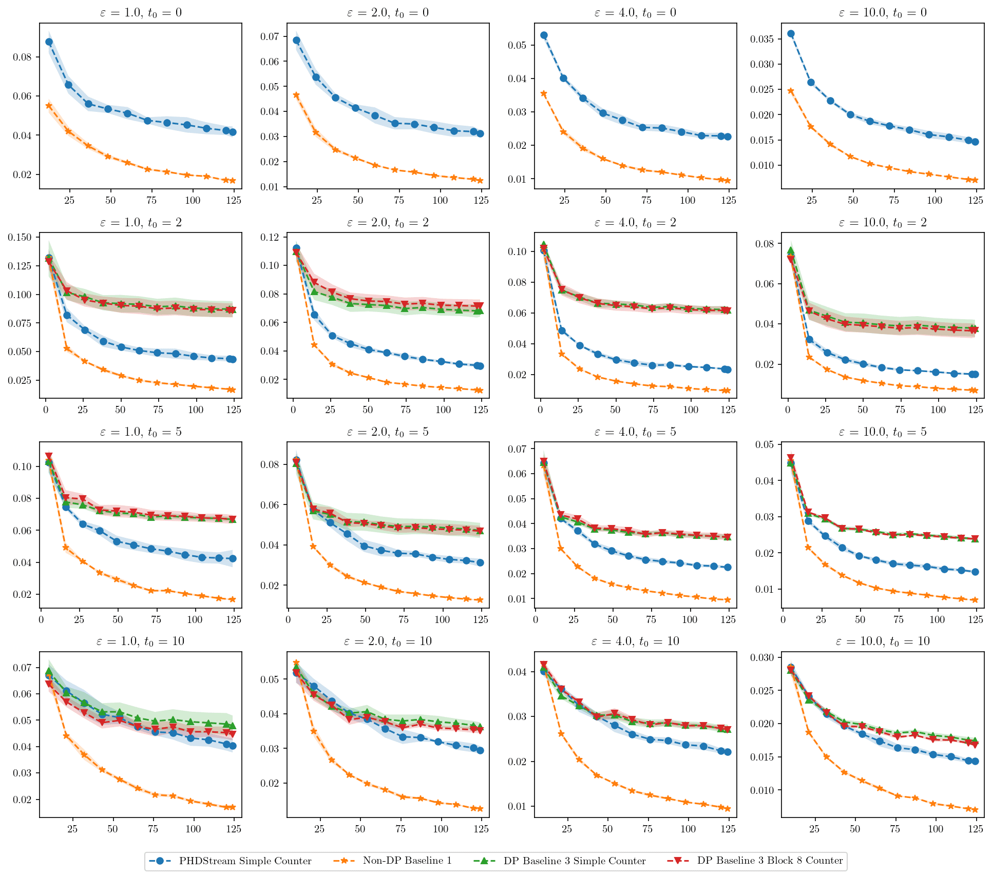
Figure 12: Query error for PHDStream over the dataset New York (over NY state) and small range queries.

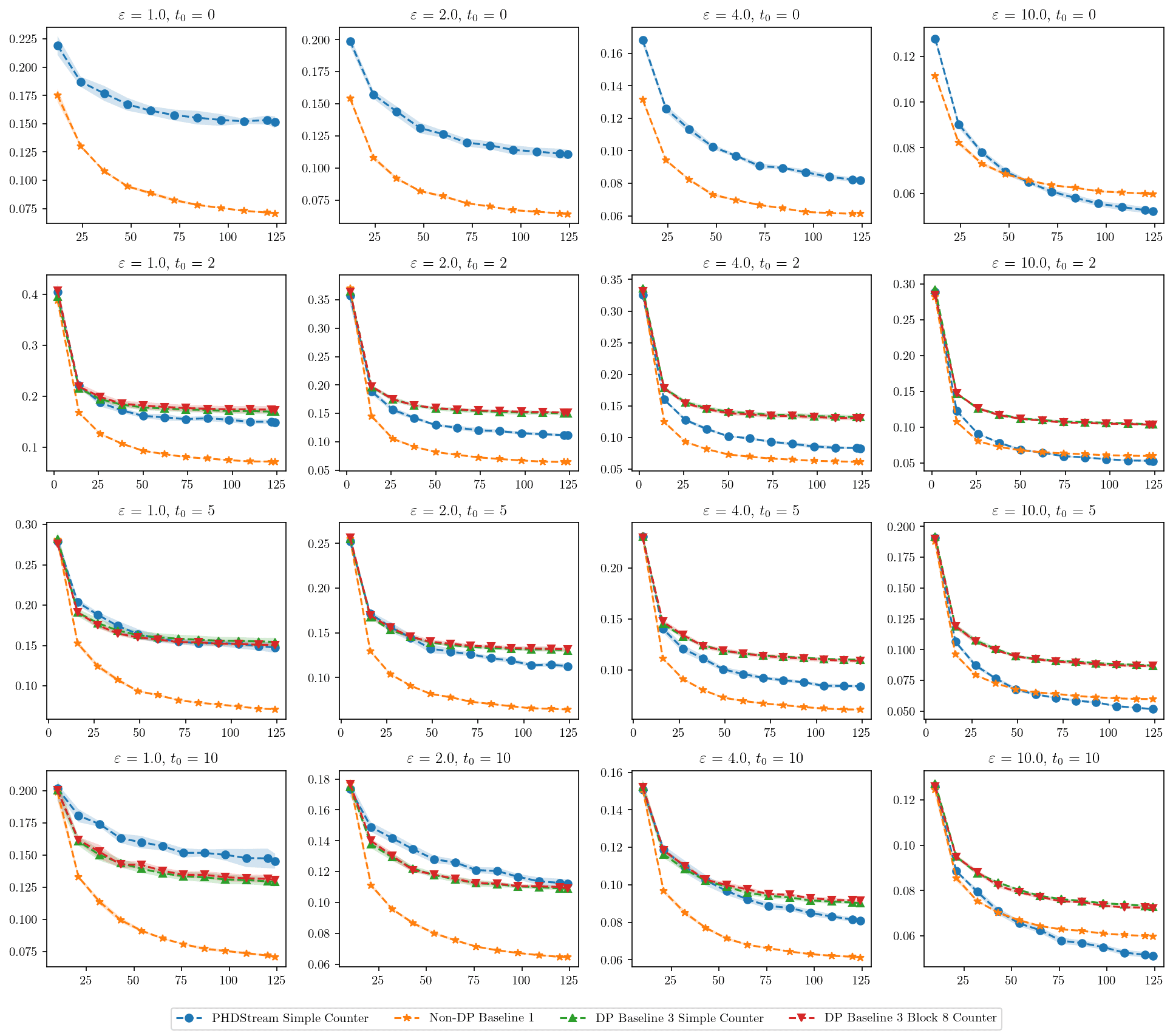
Figure 13: Query error for PHDStream over the dataset New York (over Manhattan road network) and small range queries.

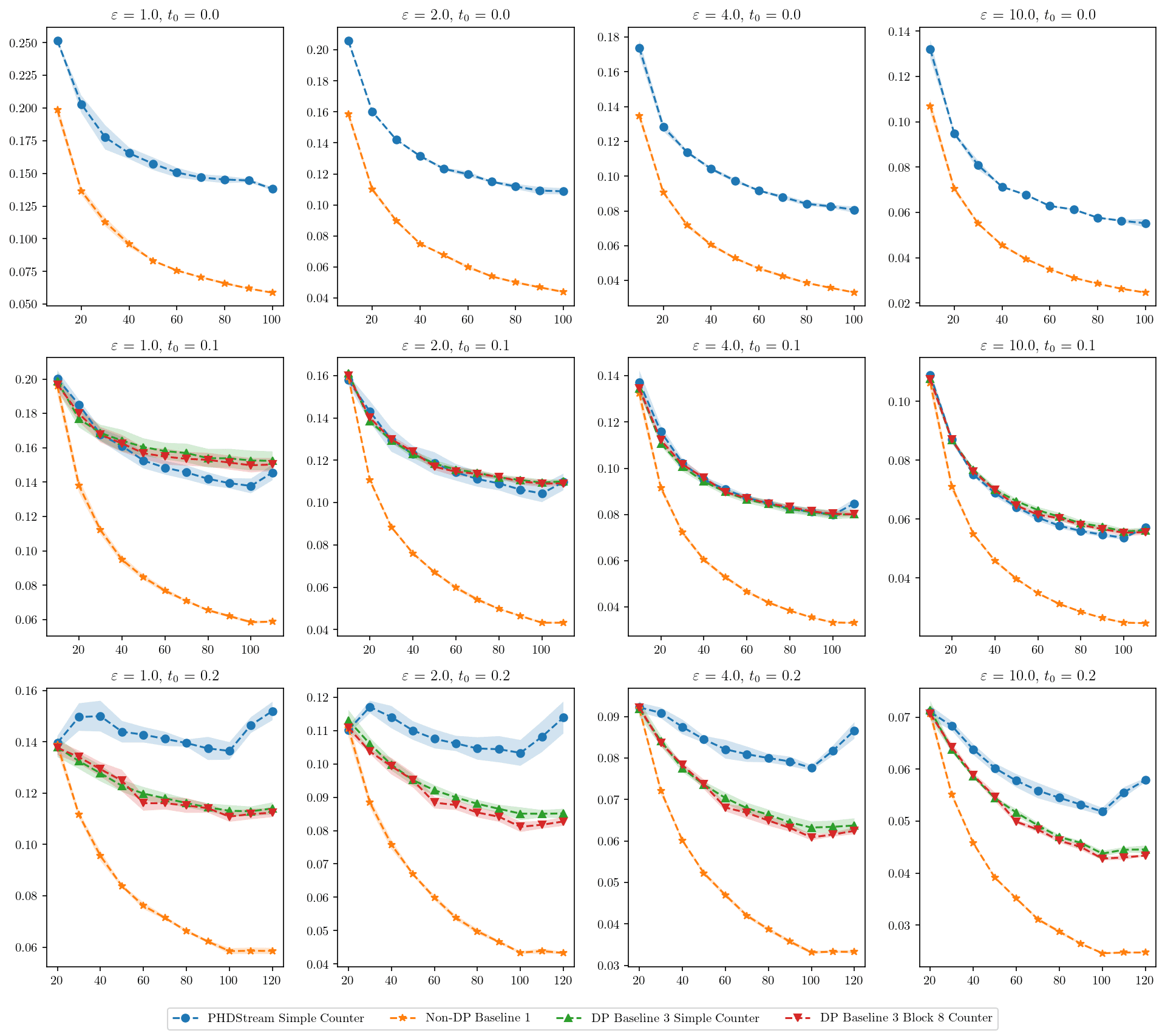
Figure 14: Query error for PHDStream over the dataset Concentric circles no deletion and small range queries.

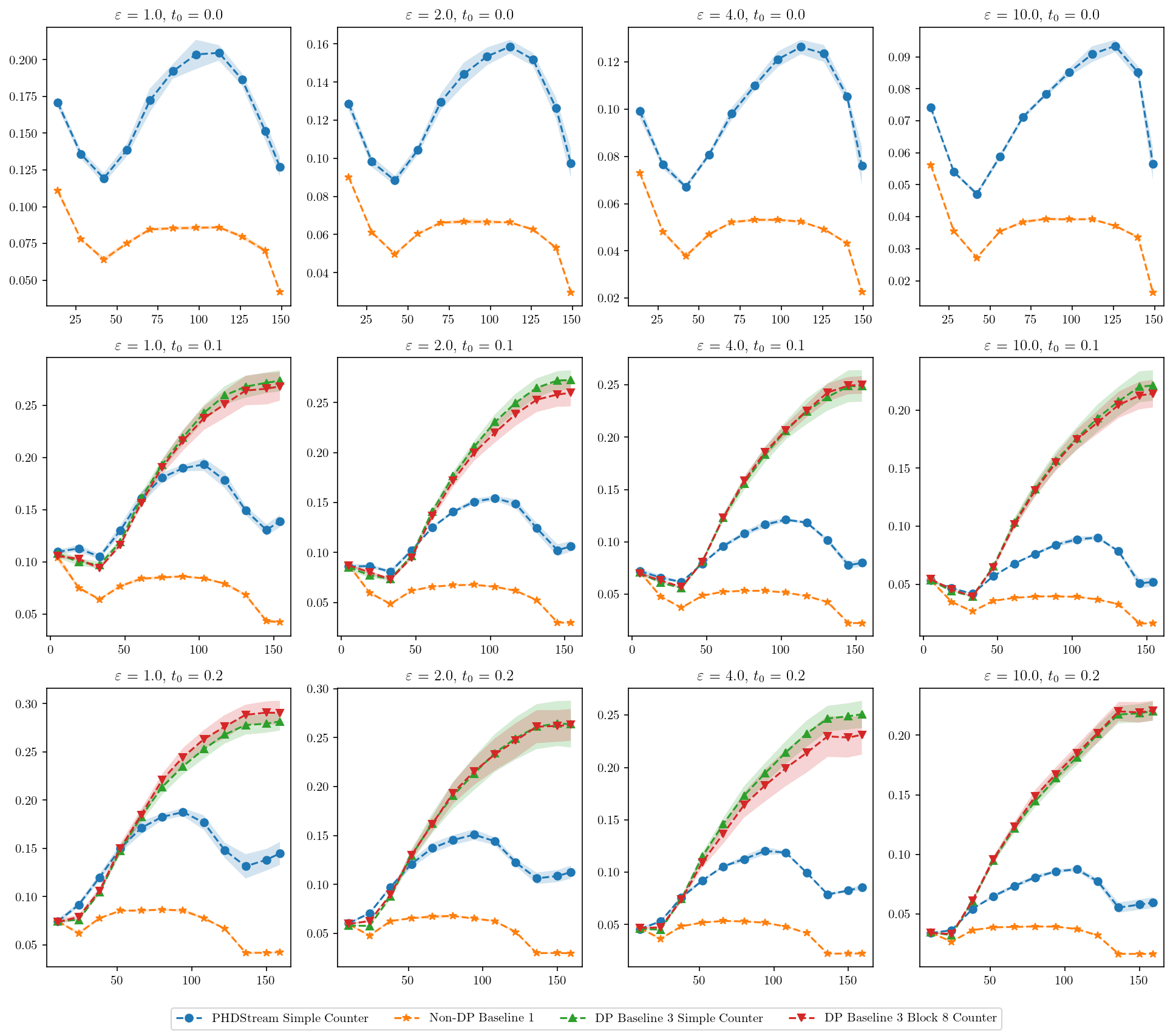
Figure 15: Query error for PHDStream over the dataset Concentric circles with deletion and small range queries.

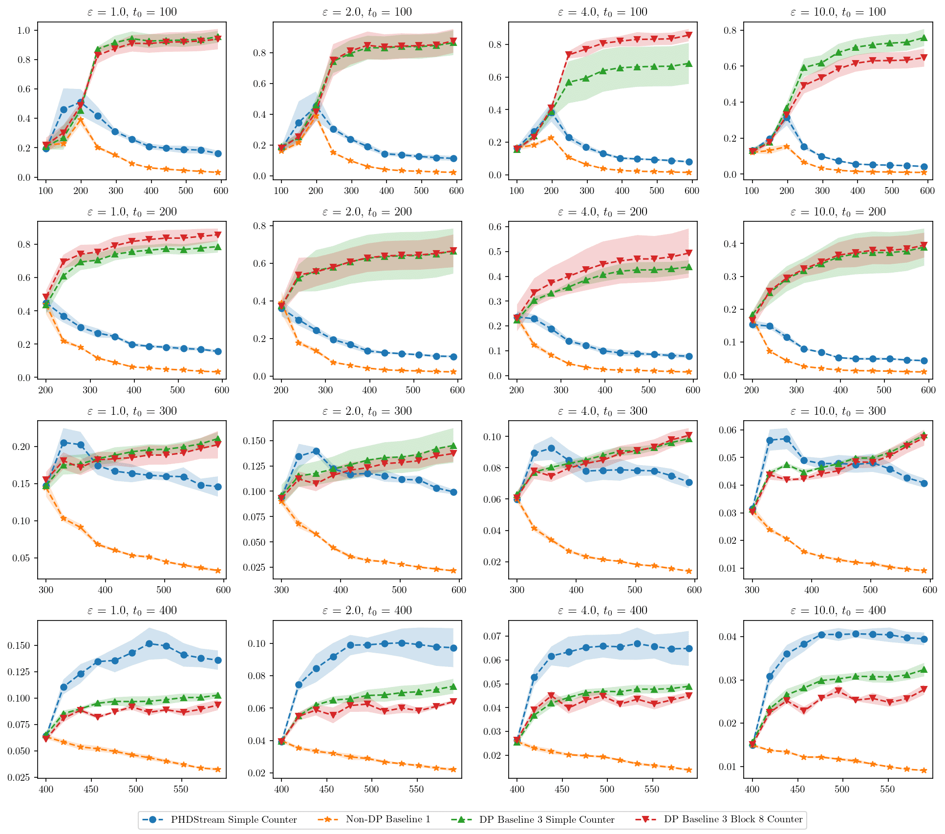
Figure 16: Query error for PHDStream over the dataset Gowalla and medium range queries.

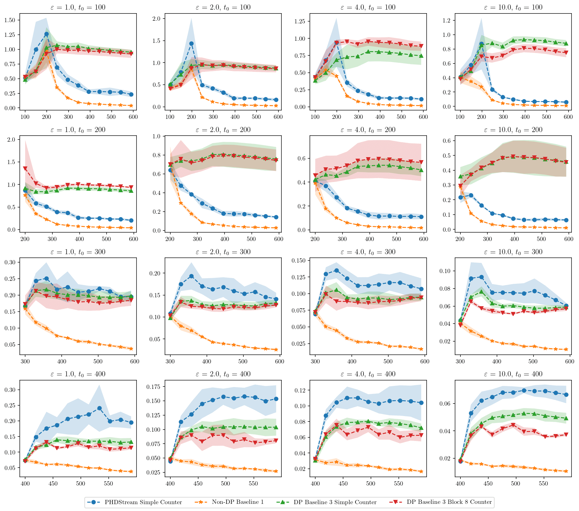
Figure 17: Query error for PHDStream over the dataset Gowalla and large range queries.

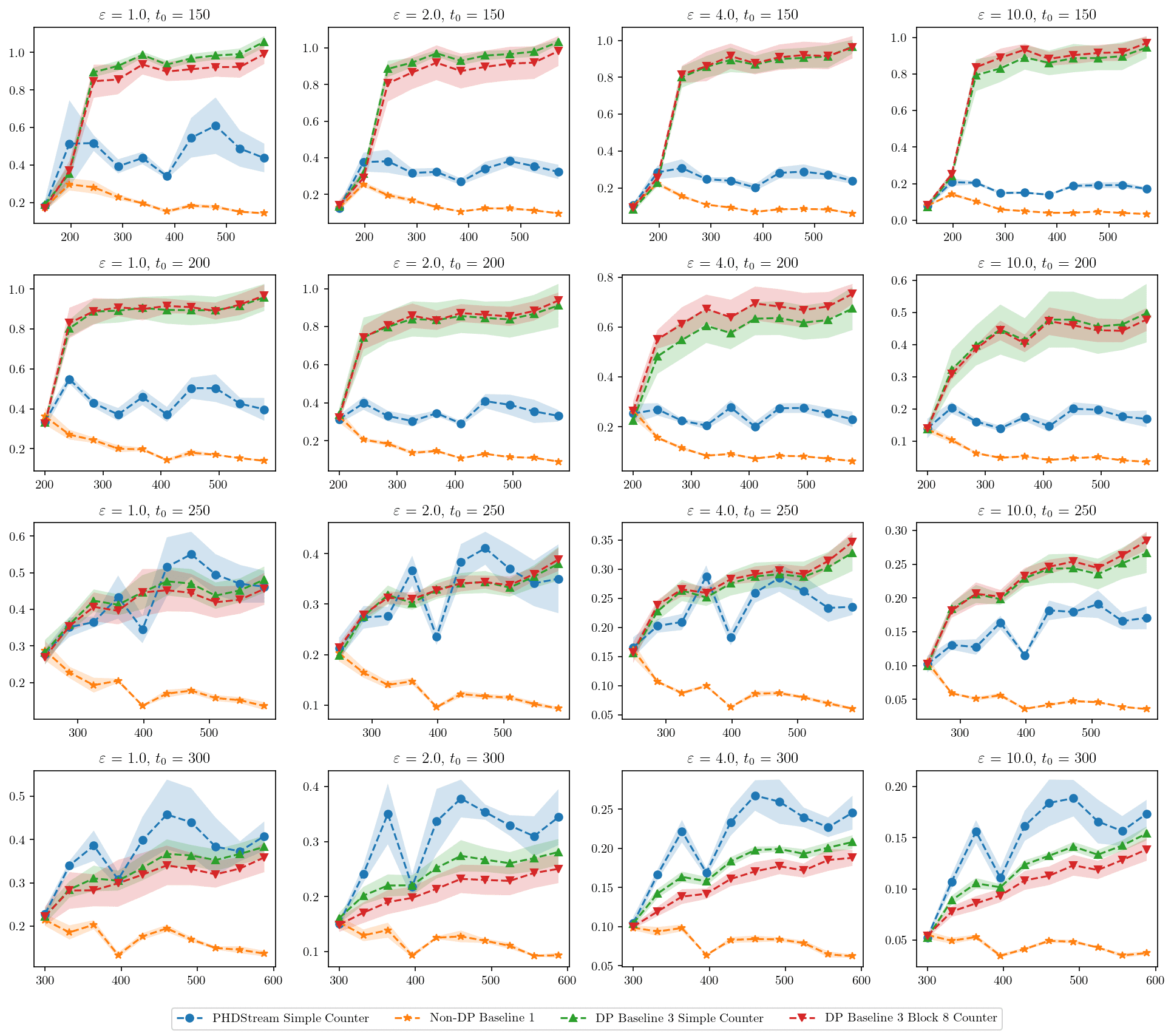
Figure 18: Query error for PHDStream over the dataset Gowalla with deletion and medium range queries.

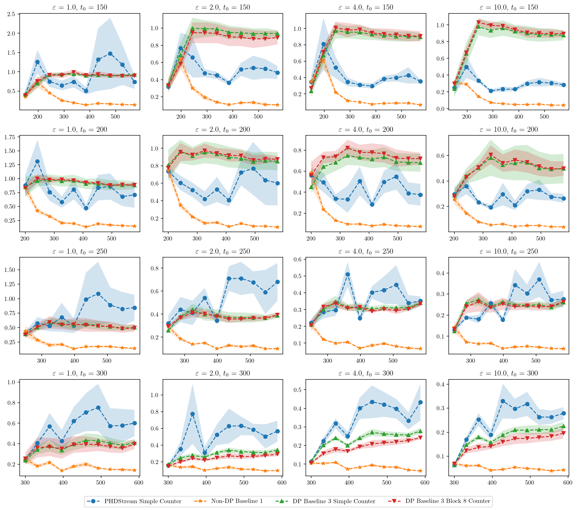
Figure 19: Query error for PHDStream over the dataset Gowalla with deletion and large range queries.

References

- loc (2021) A survey of differential privacy-based techniques and their applicability to location-based services. Computers & Security, 111:102464, 2021. ISSN 0167-4048. doi: https://doi.org/10.1016/j.cose.2021.102464. URL https://www.sciencedirect.com/science/article/pii/S0167404821002881.
- Abadi et al. (2016) Abadi, M., Chu, A., Goodfellow, I., McMahan, H. B., Mironov, I., Talwar, K., and Zhang, L. Deep learning with differential privacy. In Proceedings of the 2016 ACM SIGSAC conference on computer and communications security, pp. 308–318, 2016.
- Abowd et al. (2019) Abowd, J., Kifer, D., Garfinkel, S. L., and Machanavajjhala, A. Census topdown: Differentially private data, incremental schemas, and consistency with public knowledge. 2019.
- Bauer & Strauss (2016) Bauer, C. and Strauss, C. Location-based advertising on mobile devices: A literature review and analysis. Management review quarterly, 66(3):159–194, 2016.
- Boeing (2017) Boeing, G. Osmnx: A python package to work with graph-theoretic openstreetmap street networks. Journal of Open Source Software, 2(12):215, 2017. doi: 10.21105/joss.00215. URL https://doi.org/10.21105/joss.00215.
- Bun et al. (2023) Bun, M., Gaboardi, M., Neunhoeffer, M., and Zhang, W. Continual release of differentially private synthetic data, 2023.
- Chan et al. (2010) Chan, T.-H. H., Shi, E., and Song, D. X. Private and continual release of statistics. ACM Trans. Inf. Syst. Secur., 14:26:1–26:24, 2010.
- Chen et al. (2017) Chen, Y., Machanavajjhala, A., Hay, M., and Miklau, G. Pegasus: Data-adaptive differentially private stream processing. In Proceedings of the 2017 ACM SIGSAC Conference on Computer and Communications Security, pp. 1375–1388, 2017.
- Cho et al. (2011) Cho, E., Myers, S. A., and Leskovec, J. Friendship and mobility: User movement in location-based social networks. In Proceedings of the 17th ACM SIGKDD International Conference on Knowledge Discovery and Data Mining, KDD ’11, pp. 1082–1090, New York, NY, USA, 2011. Association for Computing Machinery. ISBN 9781450308137. doi: 10.1145/2020408.2020579. URL https://doi.org/10.1145/2020408.2020579.
- Ding et al. (2017) Ding, B., Kulkarni, J., and Yekhanin, S. Collecting telemetry data privately. In NIPS, 2017.
- Donovan & Work (2016) Donovan, B. and Work, D. New york city taxi trip data (2010-2013), 2016. URL https://doi.org/10.13012/J8PN93H8.
- Douriez et al. (2016) Douriez, M., Doraiswamy, H., Freire, J., and Silva, C. T. Anonymizing nyc taxi data: Does it matter? In 2016 IEEE international conference on data science and advanced analytics (DSAA), pp. 140–148. IEEE, 2016.
- Dwork et al. (2010) Dwork, C., Naor, M., Pitassi, T., and Rothblum, G. N. Differential privacy under continual observation. In Symposium on the Theory of Computing, 2010.
- Dwork et al. (2015) Dwork, C., Naor, M., Reingold, O., and Rothblum, G. N. Pure differential privacy for rectangle queries via private partitions. In International Conference on the Theory and Application of Cryptology and Information Security, 2015.
- Erlingsson et al. (2014) Erlingsson, U., Pihur, V., and Korolova, A. Rappor: Randomized aggregatable privacy-preserving ordinal response. In Proceedings of the 2014 ACM SIGSAC Conference on Computer and Communications Security, CCS ’14, pp. 1054–1067, New York, NY, USA, 2014. Association for Computing Machinery. ISBN 9781450329576. doi: 10.1145/2660267.2660348. URL https://doi.org/10.1145/2660267.2660348.
- Fanaeepour & Rubinstein (2018) Fanaeepour, M. and Rubinstein, B. I. P. Histogramming privately ever after: Differentially-private data-dependent error bound optimisation. In 2018 IEEE 34th International Conference on Data Engineering (ICDE), pp. 1204–1207, 2018. doi: 10.1109/ICDE.2018.00111.
- Gillies et al. (2023) Gillies, S., van der Wel, C., Van den Bossche, J., Taves, M. W., Arnott, J., Ward, B. C., and others. Shapely, January 2023. URL https://github.com/shapely/shapely.
- Guha Thakurta & Smith (2013) Guha Thakurta, A. and Smith, A. (nearly) optimal algorithms for private online learning in full-information and bandit settings. In Burges, C., Bottou, L., Welling, M., Ghahramani, Z., and Weinberger, K. (eds.), Advances in Neural Information Processing Systems, volume 26. Curran Associates, Inc., 2013. URL https://proceedings.neurips.cc/paper_files/paper/2013/file/c850371fda6892fbfd1c5a5b457e5777-Paper.pdf.
- Hagberg et al. (2008) Hagberg, A. A., Schult, D. A., and Swart, P. J. Exploring network structure, dynamics, and function using networkx. In Varoquaux, G., Vaught, T., and Millman, J. (eds.), Proceedings of the 7th Python in Science Conference, pp. 11 – 15, Pasadena, CA USA, 2008.
- Hardt et al. (2012) Hardt, M., Ligett, K., and McSherry, F. A simple and practical algorithm for differentially private data release. Advances in neural information processing systems, 25, 2012.
- Jain et al. (2023) Jain, P., Kalemaj, I., Raskhodnikova, S., Sivakumar, S., and Smith, A. Counting distinct elements in the turnstile model with differential privacy under continual observation, 2023.
- Jin et al. (2023) Jin, F., Hua, W., Francia, M., Chao, P., Orlowska, M. E., and Zhou, X. A survey and experimental study on privacy-preserving trajectory data publishing. IEEE Transactions on Knowledge and Data Engineering, 35(6):5577–5596, 2023. doi: 10.1109/TKDE.2022.3174204.
- Jordahl et al. (2020) Jordahl, K., den Bossche, J. V., Fleischmann, M., Wasserman, J., McBride, J., Gerard, J., Tratner, J., Perry, M., Badaracco, A. G., Farmer, C., Hjelle, G. A., Snow, A. D., Cochran, M., Gillies, S., Culbertson, L., Bartos, M., Eubank, N., maxalbert, Bilogur, A., Rey, S., Ren, C., Arribas-Bel, D., Wasser, L., Wolf, L. J., Journois, M., Wilson, J., Greenhall, A., Holdgraf, C., Filipe, and Leblanc, F. geopandas/geopandas: v0.8.1, July 2020. URL https://doi.org/10.5281/zenodo.3946761.
- Jordon et al. (2019) Jordon, J., Yoon, J., and Van Der Schaar, M. Pate-gan: Generating synthetic data with differential privacy guarantees. In International conference on learning representations, 2019.
- Joseph et al. (2018) Joseph, M., Roth, A., Ullman, J., and Waggoner, B. Local differential privacy for evolving data. In Neural Information Processing Systems, 2018.
- Kairouz et al. (2021) Kairouz, P., Mcmahan, B., Song, S., Thakkar, O., Thakurta, A., and Xu, Z. Practical and private (deep) learning without sampling or shuffling. In Meila, M. and Zhang, T. (eds.), Proceedings of the 38th International Conference on Machine Learning, volume 139 of Proceedings of Machine Learning Research, pp. 5213–5225. PMLR, 18–24 Jul 2021. URL https://proceedings.mlr.press/v139/kairouz21b.html.
- Kim et al. (2018) Kim, J. S., Chung, Y. D., and Kim, J. W. Differentially private and skew-aware spatial decompositions for mobile crowdsensing. Sensors, 18(11):3696, 2018.
- Lee et al. (2008) Lee, J., Shin, I., and Park, G.-L. Analysis of the passenger pick-up pattern for taxi location recommendation. In 2008 Fourth international conference on networked computing and advanced information management, volume 1, pp. 199–204. IEEE, 2008.
- Li et al. (2017) Li, M., Zhu, L., Zhang, Z., and Xu, R. Achieving differential privacy of trajectory data publishing in participatory sensing. Information Sciences, 400:1–13, 2017.
- Li et al. (2021) Li, X., Tramer, F., Liang, P., and Hashimoto, T. Large language models can be strong differentially private learners. arXiv preprint arXiv:2110.05679, 2021.
- McKenna et al. (2021a) McKenna, R., Miklau, G., Hay, M., and Machanavajjhala, A. Hdmm: Optimizing error of high-dimensional statistical queries under differential privacy. arXiv preprint arXiv:2106.12118, 2021a.
- McKenna et al. (2021b) McKenna, R., Miklau, G., and Sheldon, D. Winning the nist contest: A scalable and general approach to differentially private synthetic data. Journal of Privacy and Confidentiality, 11(3), 2021b.
- Ni et al. (2018) Ni, L., Li, C., Wang, X., Jiang, H., and Yu, J. Dp-mcdbscan: Differential privacy preserving multi-core dbscan clustering for network user data. IEEE access, 6:21053–21063, 2018.
- Qardaji et al. (2013) Qardaji, W., Yang, W., and Li, N. Differentially private grids for geospatial data. In 2013 IEEE 29th international conference on data engineering (ICDE), pp. 757–768. IEEE, 2013.
- Sarathy & Vadhan (2022) Sarathy, J. and Vadhan, S. Analyzing the differentially private theil-sen estimator for simple linear regression. arXiv preprint arXiv:2207.13289, 2022.
- Tang et al. (2017) Tang, J., Korolova, A., Bai, X., Wang, X., and Wang, X. Privacy loss in apple’s implementation of differential privacy on macos 10.12, 2017.
- Tao et al. (2021) Tao, Y., McKenna, R., Hay, M., Machanavajjhala, A., and Miklau, G. Benchmarking differentially private synthetic data generation algorithms. arXiv preprint arXiv:2112.09238, 2021.
- Team (2017) Team, D. P. Learning with privacy at scale. Technical report, Apple, December 2017. URL https://machinelearning.apple.com/research/learning-with-privacy-at-scale.
- Torkzadehmahani et al. (2019) Torkzadehmahani, R., Kairouz, P., and Paten, B. Dp-cgan: Differentially private synthetic data and label generation. In Proceedings of the IEEE/CVF Conference on Computer Vision and Pattern Recognition Workshops, pp. 0–0, 2019.
- Wang et al. (2021) Wang, T., Chen, J. Q., Zhang, Z., Su, D., Cheng, Y., Li, Z., Li, N., and Jha, S. Continuous release of data streams under both centralized and local differential privacy. In Proceedings of the 2021 ACM SIGSAC Conference on Computer and Communications Security, pp. 1237–1253, 2021.
- Wikipedia contributors (2017) Wikipedia contributors. Weather (Apple) — Wikipedia, the free encyclopedia, 2017. URL https://en.wikipedia.org/wiki/Weather_(Apple). [Online; accessed 02-June-2023].
- Xu et al. (2019) Xu, C., Ren, J., Zhang, D., Zhang, Y., Qin, Z., and Ren, K. Ganobfuscator: Mitigating information leakage under gan via differential privacy. IEEE Transactions on Information Forensics and Security, 14(9):2358–2371, 2019.
- Xu et al. (2017) Xu, F., Tu, Z., Li, Y., Zhang, P., Fu, X., and Jin, D. Trajectory recovery from ash: User privacy is not preserved in aggregated mobility data. In Proceedings of the 26th International Conference on World Wide Web, WWW ’17, pp. 1241–1250, Republic and Canton of Geneva, CHE, 2017. International World Wide Web Conferences Steering Committee. ISBN 9781450349130. doi: 10.1145/3038912.3052620. URL https://doi.org/10.1145/3038912.3052620.
- Yue et al. (2022) Yue, X., Inan, H. A., Li, X., Kumar, G., McAnallen, J., Sun, H., Levitan, D., and Sim, R. Synthetic text generation with differential privacy: A simple and practical recipe. arXiv preprint arXiv:2210.14348, 2022.
- Zhang et al. (2016) Zhang, J., Xiao, X., and Xie, X. Privtree: A differentially private algorithm for hierarchical decompositions. Proceedings of the 2016 International Conference on Management of Data, 2016.
- Zhang et al. (2017) Zhang, J., Cormode, G., Procopiuc, C. M., Srivastava, D., and Xiao, X. Privbayes: Private data release via bayesian networks. ACM Transactions on Database Systems (TODS), 42(4):1–41, 2017.
- Zhang et al. (2012) Zhang, M., Liu, J., Liu, Y., Hu, Z., and Yi, L. Recommending pick-up points for taxi-drivers based on spatio-temporal clustering. In 2012 Second International Conference on Cloud and Green Computing, pp. 67–72. IEEE, 2012.