From square plaquettes to triamond lattices for SU(2) gauge theory
Abstract
Lattice gauge theory should be able to address significant new scientific questions when implemented on quantum computers. In practice, error-mitigation techniques have already allowed encouraging progress on small lattices. In this work we focus on a truncated version of SU(2) gauge theory, which is a familiar non-Abelian step toward quantum chromodynamics. First, we demonstrate effective error mitigation for imaginary time evolution on a lattice having two square plaquettes, obtaining the ground state using an IBM quantum computer and observing that this would have been impossible without error mitigation. Then we propose the triamond lattice as an expedient approach to lattice gauge theories in three spatial dimensions, deriving the Hamiltonian and obtaining energy eigenvalues and eigenstates from a noiseless simulator for a three-dimensional unit cell.
I Introduction
Quantum field theory combines quantum mechanics with special relativity and is of widespread importance in high-energy physics, nuclear physics, and condensed matter physics. Enforcing a spatially local symmetry leads to the special case of a gauge theory. The standard model of particle physics is a collection of three gauge theories describing the strong, weak and electromagnetic forces. Because perturbation theory cannot be applied to a large coupling constant, many aspects of the strong force are best described by a numerical approach called lattice gauge theory.
Lattice gauge theory has been of central importance to quantum chromodynamics for several decades and has become a precision tool for practitioners [1, 2]. It provides rigorous calculations of static properties, such as the masses and form factors of hadrons, directly from the gauge theory of quarks and gluons. Such calculations are crucial in the ongoing quest to understand hadron physics, such as the tetraquarks and pentaquarks that have been discovered experimentally in recent years [3, 4]. Lattice gauge theory calculations also provide necessary input for experiments seeking new physics beyond the standard model, where a famous recent example is the anomalous magnetic moment of the muon [5].
Quantum computers offer a prospective way to calculate more than just static properties. Traditional lattice gauge theory uses Monte Carlo methods that would have sign problems if applied straightforwardly to situations involving dynamics, nonzero density, or some topological interactions [6, 7]. These sign problems can be avoided by using a Hamiltonian approach, where the exponentially large Hilbert space can fit naturally onto a quantum computer. Now that quantum computing hardware is becoming a reality, this powerful new approach to lattice gauge theory is being developed by a broad community of researchers [7, 8, 9].
With quantum chromodynamics as a motivating long-range goal, the present work is focused on the simplest non-Abelian gauge theory. Being non-Abelian means that gauge fields carry the relevant charge directly and can therefore interact among themselves, like the gluons of quantum chromodynamics and in contrast to the photons of quantum electrodynamics. Specifically our work will consider SU(2) gauge theory in the absence of fermions, and we will truncate the gauge field to fit on a small number of qubits. Several research groups have already carried out exploratory studies of non-Abelian gauge theories on quantum computing hardware [10, 11, 12, 13, 14, 15, 16, 17, 18, 19, 20, 21]. There have also been many theoretical studies laying the groundwork for anticipated implementations on larger quantum computers [22, 23, 24, 25, 26, 27, 28, 29, 30, 31, 32, 33, 34, 35, 36, 37, 38, 39, 40, 41, 42, 43, 44, 45, 46, 47, 48, 49, 50, 51, 52, 53, 54, 55, 56, 57, 58, 59, 60, 61]. In the present work, we address two important issues: an effective way to mitigate errors and a practical way to extend lattices into three spatial dimensions.
Future quantum computers are expected to have smaller error rates and robust methods for correcting those errors, but calculations in the present era face substantial error rates and typically have insufficient resources to implement true error correction. Instead, error mitigation methods have been devised [62], and these can provide significant improvements for computations performed on today’s hardware. Our study demonstrates the use of an existing method called self-mitigation [17] but in a new context: evolution of a quantum state through imaginary time. As is well known, after sufficiently many steps of imaginary time the excited state contributions to a generic initial state will become exponentially suppressed relative to the ground state, thus providing a way to create the ground state and to determine its eigenvalue. Our results will demonstrate that self-mitigation correctly finds and sustains the true ground state of a two-plaquette lattice even though the unmitigated data points are moving ever farther from the true result with each additional time step.
With successful mitigation in hand, we then turn our attention to lattice gauge theory in three spatial dimensions. While this can be done with a standard cubic lattice, it is important to remember that whenever more than three gauge links meet at a lattice site, the quantum numbers of the gauge links themselves are insufficient to fully define the state of the gauge field across the lattice [36, 40, 54, 58]. For example, consider four SU(2) gauge links meeting at a site and suppose each gauge link has quantum number , where is notation familiar from quantized angular momentum though here it refers to the gauge degrees of freedom. One pair of these links could sum to or . The other pair must have the same sum because Gauss’s law requires the total of all four to be . Therefore a full description of the state requires not just the values of individual links, but also the value of for some pair selected by the user to define that site.
One way to handle this issue is to assign a sufficient number of additional qubits at each lattice site, being careful to define a convention at each site, thereby completing the state’s definition [36, 40, 54, 58]. In the present work we propose an alternative based on a structure from crystallography [63, 64, 65, 66, 67, 68]. Having only three links at each site, our choice will avoid the need for any quantum numbers beyond the individual link values.
Consider a lattice where each site is touched by exactly three gauge links that have equal lengths, lie in a single plane, and are placed at equal angles around the site, i.e. . This forms a three-dimensional lattice that has a high degree of symmetry and needs no additional qubits beyond the links themselves. Because of its similarity to a diamond crystal of carbon atoms but with three links per site instead of four, it has been called the triamond lattice [66, 67]. It is also known as the Laves lattice [64] or the lattice [65, 68]. In this work, we provide an introduction to lattice gauge theory on the triamond framework. We derive the SU(2) Hamiltonian for a triamond lattice and demonstrate its use on a noiseless simulator.
II Results
II.1 Imaginary time evolution on square plaquettes
Finding the ground state for a given Hamiltonian is an important ingredient of many scientific studies. Two common approaches are variational methods and imaginary time evolution. Variational methods rely on an ansatz chosen by the user, and can only get as close to the true ground state as the ansatz will allow. In contrast, imaginary time evolution always converges to the true ground state unless the initial state is perfectly orthogonal to it.
Imaginary time evolution is used routinely in traditional lattice gauge theory on classical computers. Our motivation to study it now on a quantum computer is not to compete with successful classical methods, but rather to imagine that ground-state preparation will become the first step in a larger computation that truly does require quantum computing [69, 70].
Our computation uses a lattice comprising two side-by-side square plaquettes that share a single gauge link, thus forming a left path, a center path, and a right path as shown in Fig. 1. Each of the seven gauge links on this lattice is a superposition of SU(2) representations, and Gauss’s law requires the three on the left path to equal one another and similarly the three on the right path must equal one another. For our calculation we truncate the basis and retain only the two lowest states for each gauge link, and .
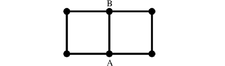
Any state of this system can be described by two qubits, one for the left path and one for the right path, because Gauss’s law then determines the center path uniquely. Such a tiny system is a valuable place to study error mitigation because a single time step requires only a simple circuit while more and more time steps will require more and more entangling gates. The real-time evolution of this system was studied previously as the first example of self-mitigation [17]. The Hamiltonian, in units of , is
| (1) | |||||
where and is the coupling constant, i.e. the strength of the strong interaction for this physics theory. The Pauli gates acting on qubit are , and .
Imaginary time evolution is not a unitary operation, so how can it be implemented on a quantum computer? We use an algorithm developed by Motta et al., called quantum imaginary time evolution (QITE) [71], which can be described as follows. The evolution we seek is
| (2) |
where is the real-valued Euclidean time parameter. We can define a normalized state such that for positive . The evolution can always be expressed as
| (3) |
for some unitary operator and positive . An immediate consequence is
| (4) |
The operator can be determined from a state tomography of that reflects the specific qubit connectivities of .
For our physics example, Eq. (1) confirms that the Hamiltonian is purely real, meaning that we can restrict ourselves to real-valued basis states as well. Together with Eqs. (2) and (3), this realness means must be purely imaginary, leading to a general expression with odd powers of gates,
| (5) | |||||
The state tomography that determines the values of the coefficients is presented in Sec. IV.1. With those values in hand, and with obtained from the calculation of Eq. (4), the state at a small value of can be computed from Eq. (3). In particular, we use
| (6) | |||||
| (7) | |||||
| (8) |
where is a CNOT gate with qubit as control and qubit as target.
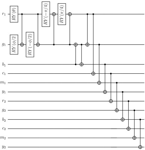
For sufficiently small , the operator can be approximated by a product of six factors, one for each term in . For a better approximation, that first-order Trotter expression can be replaced by the second-order Trotter expression represented by the circuit shown in Fig. 2. To reach a larger value of , we can perform a sequence of small steps where the circuit is several end-to-end copies of Fig. 2. Notice that the tomography needs to be computed separately for each step, using the state at the previous step as input.
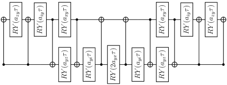
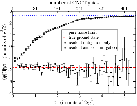
Because the two-qubit CNOT gate is noisier than a single-qubit gate on quantum hardware, the gates in Fig. 2 have been ordered in a way that minimizes the number of CNOT gates. Also, the CNOT gate at the end of one Trotter step will cancel the CNOT gate at the beginning of the next step. As well, the very first CNOT gate in the circuit can be omitted because the initial control qubit is always off. Nevertheless, the open symbols in Fig. 3 show that only the first two or three time steps approach the true ground state energy and then subsequent time steps move further and further away. The quantum computation is overwhelmed by hardware noise without ever reaching the correct result.
Self-mitigation is able to extract the true result from the computed data. The original implementation [17], which was inspired by the work of Urbanek et al. [72], has subsequently been used and extended in various ways [18, 19, 21, 56, 73, 74, 75, 76, 70, 77]. The basic idea is to run a mitigation circuit that is identical to the physics circuit except that in the second half of the circuit. If your circuit has an odd number of second-order Trotter steps, use in the center gate (see, for example, Fig. 2) and insert a barrier to prevent CNOT cancellation.
The true outcome of the mitigation circuit should be identical to the initial state, i.e. all qubits should be in the off position. Comparison of the computed results with this known true result provides a measurement of hardware errors. The physics circuit will have similar hardware errors because the two circuits are identical up to the sign of in the latter half.
More precisely, randomized compiling (see Sec. IV.2) is used to convert CNOT errors into incoherent noise that is well described by the depolarizing noise model [72]. For our example of imaginary time evolution, this leads to a pair of ratios,
| (9) |
| (10) |
where . These equations give the true expectation value of a Pauli string as the ratio of results computed by a physics run and a mitigation run. They are the counterparts of Eq. (8) in the original paper [17] but look slightly different because the previous work studied probabilities that equalled in the pure noise limit whereas the present work employs expectation values of Pauli strings that are zero for pure noise.
The filled data points of Fig. 3 were obtained by computing each term of Eq. (1) from the ratios in Eqs. (9) and (10). The physics runs and mitigation runs (with 50 randomized compilings for each) and the readout error mitigation runs were all completed within a single qiskit job [78] to ensure they were experiencing the same hardware conditions. Whereas the unmitigated data points in Fig. 3 approach the pure noise limit of , where only the first term in Eq. (1) makes a nonzero contribution, the self-mitigated data points in Fig. 3 remain consistent with the true ground state as increases. Error bars grow as the circuit gets longer, but meaningful results are still obtained with more than 400 CNOT gates. This success provides an incentive to move toward larger lattices, including novel three-dimensional approaches like the triamond lattice.
II.2 The SU(2) Hamiltonian for a triamond lattice
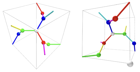
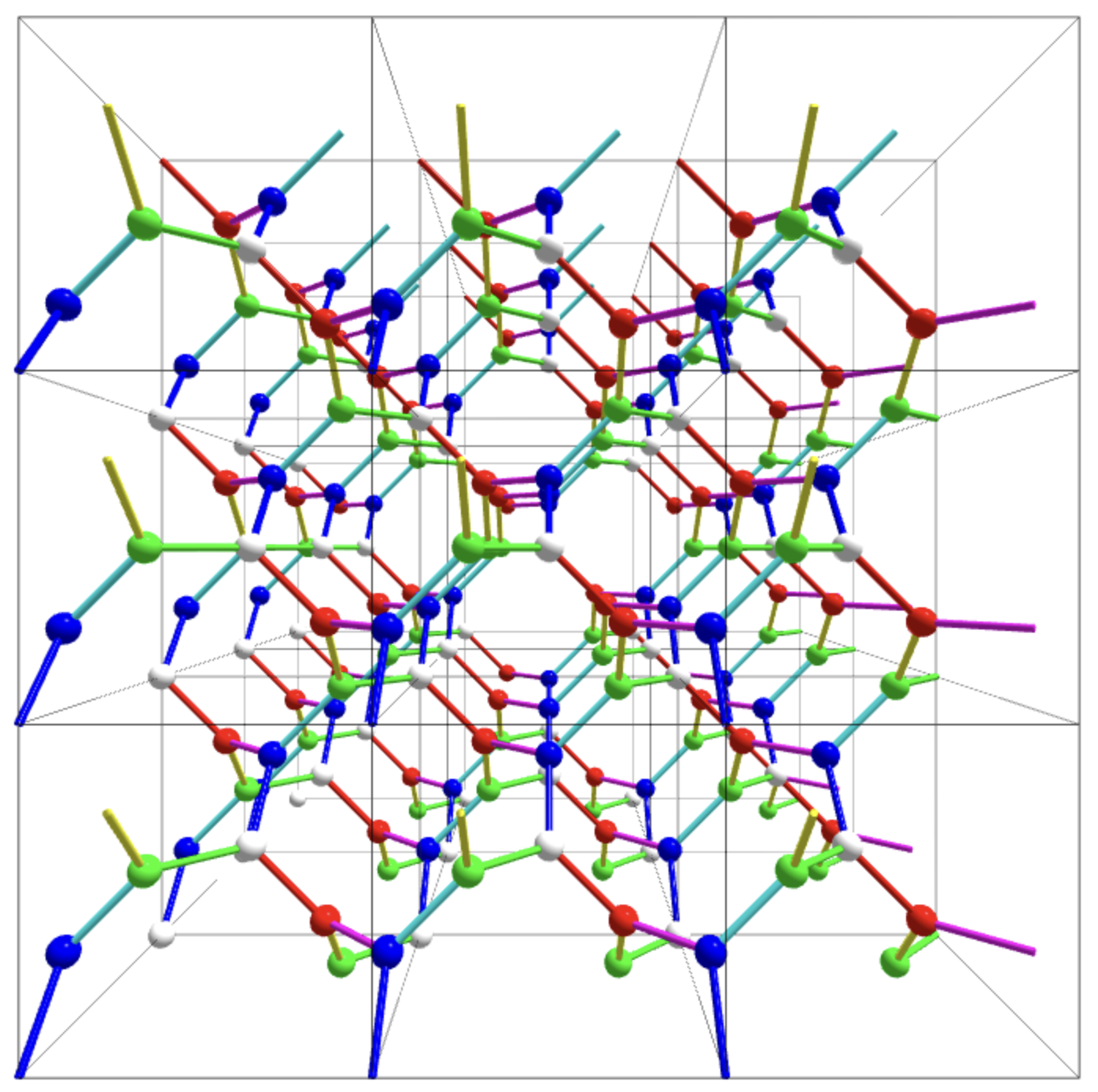
Figs. 4 and 5 show the locations of lattice sites and gauge links on a triamond lattice. See also our two-minute video presentation [79], which provides views of the triamond lattice from a camera moving around it.
To introduce the triamond lattice quantitatively, we will first define six unit vectors labeled as colors (red, green, blue, cyan, magenta, yellow) to aid the discussion,
| (11) |
| (12) |
where , and are the standard orthonormal vectors. Every gauge link in the triamond lattice is along one of these color directions. As an aside, we note that the colors defined here have nothing to do with the colors of quantum chromodynamics.
Each lattice site is touched by three gauge links that lie in a plane. The complete lattice has just four sets of parallel planes, so we color each site white, red, green or blue to represent which plane is at that site. The links and sites form a color scheme that is motivated by the well-known RGB model of colors: each white site is touched by red, green and blue links, each red site is touched by red, magenta and yellow links, each green site is touched by green, cyan and yellow links, and each blue site is touched by blue, cyan and magenta links.
The angle between any two planes is , which is familiar because this same angle lies between any pair of lines joining the center of a cube to neighboring corners. Because the unit vector orthogonal to a plane is only unique up to its sign, the triamond lattice is chiral. Specifically, the mirror image of Fig. 5 is a distinct but equally valid triamond lattice.
Notice that the white sites of a triamond lattice form a body-centered cubic (bcc) structure. It is useful to compare the options of defining a lattice gauge theory on a triamond lattice, on a bcc lattice, or on a simple cubic lattice. Relative to a simple cubic lattice of the same volume, a bcc lattice has twice as many lattice sites, gauge links that are shorter by a factor of , and each bcc site has 8 nearest neighbors compared to 6 for the simple cubic lattice. This suggests that a bcc lattice could be valuable for efficient discussions of the continuum limit, perhaps alongside simple cubic studies. Importantly, the bcc and simple cubic lattices both have more than three gauge links touching each lattice site, meaning that extra qubits would be needed within each lattice site (and a convention must be chosen) to fully define the quantum state of the lattice [36, 40, 54]. In a sense, the triamond lattice can be viewed as a bcc lattice where those implicit qubits have been made explicit and unambiguous by creating the red, green and blue sites.
Although the white sites do form a bcc lattice, the triamond lattice is more economical than merely being a clarified bcc lattice. Imagine, for example, shrinking the red, green and blue links into their white sites. The remaining lattice would not be bcc because it would have only 6 links per unit cell (2 cyan, 2 magenta, and 2 yellow) whereas a bcc lattice would require 8 links per unit cell.
The comparison to bcc is encouraging, but our primary motivation for proposing the triamond lattice is the fact that it has exactly three links touching each site, so the values of each gauge link are sufficient to define basis states for the lattice. For planar physics, a hexagonal lattice succeeds in having three links touching each site, and SU(2) gauge theory has recently been implemented on a hexagonal lattice [58, 60]. Notice that the shortest closed paths on a hexagonal lattice have six gauge links.
The shortest closed paths on a triamond lattice have 10 gauge links. We refer to these as elementary plaquettes. Among the 10 gauge links comprising any elementary plaquette, one of the 6 colors is absent and the other 5 colors always occur twice. The lattice has only 6 orientations of plaquettes (the non-red plaquette, the non-green plaquette, etc.), with copies of them translated spatially throughout the lattice.
To perform any quantum computation on a triamond lattice, we need a Hamiltonian. For SU(2) gauge theory, the Hamiltonian is the non-Abelian generalization of quantum electrodynamics and is written as a sum of electric terms and magnetic terms [22]. In the continuum limit, the Hamiltonian is
| (13) | |||||
| (14) | |||||
| (15) |
where each trace is over the SU(2) indices of the electric field or field strength tensor .
On a lattice, each gauge link is an element of SU(2),
| (16) |
and the component of the gauge field at site that points in direction is an element of the SU(2) algebra,
| (17) |
Our computations will be performed in the electric basis, where the magnetic terms are best expressed as a sum of all elementary plaquettes in this lattice and each plaquette is the trace of the ordered product of the 10 gauge links comprising that plaquette. The somewhat tedious derivation of this lattice Hamiltonian is outlined in Sec. IV.3. The result is
| (18) | |||||
| (19) | |||||
| (20) |
where the lattice spacing is defined to be the distance between nearest-neighbor sites, i.e. the length of each gauge link on the lattice. The sum in over 6 plaquettes, , for each white lattice site includes all plaquettes on the lattice. Specifically, there is one of each type of plaquette (non-red, non-green, etc.) associated with each white site, and we use the subscript to identify the color that is absent from the plaquette.
Any eigenstate of is fully defined by providing the quantum numbers for every gauge link on the triamond lattice, , , , …. Our shorthand for an eigenstate is . The diagonal matrix elements of the Hamiltonian are
| (21) |
and the off-diagonal matrix elements from initial state to final state come from Eq. (20) with
| (24) | |||||
where the right-hand side has a standard symbol and the product includes the 10 sites in order around the plaquette. For SU(2), either direction around the plaquette gives the same result. There are three links at each site, one external to the plaquette (subscript ), one in the forward direction around the plaquette (subscript ), and one in the backward direction around the plaquette (subscript ). Eq. (24) is not specific to the triamond lattice and has been obtained previously by other authors [54, 55].
II.3 Computations on the triamond unit cell
As shown in Fig. 4, a unit cell contains 12 gauge links. By using periodic boundary conditions, a single unit cell becomes a viable three-dimensional lattice having exactly three gauge links touching each site. If each SU(2) gauge link is truncated to just two basis states, and , the unit cell accommodates basis states.
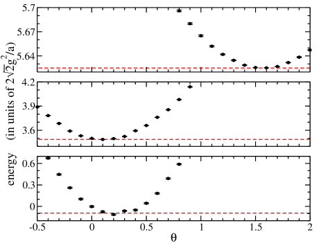
A simple way to begin exploring this theory is to use the variational method, which will find the lowest energy state among all states that couple to a selected ansatz. Fig. 6 shows three energy eigenstates obtained from three different ansatze, each having just one variational parameter. (We name the parameter in every case, but they are three different parameters.) Each of these examples is successful in finding a true eigenstate of the Hamiltonian. The 12-qubit quantum circuits that produced these results can be found in Sec. IV.4.
To gain more intuition, notice that there is no 10-sided path inside a unit cell. This means any plaquette operator will wrap around the lattice and touch one of the gauge links twice, thus changing that value of twice. With our truncation to , this means only 8 gauge links are changed when a plaquette operator is applied to the single-cell lattice.
For example, begin with on all 12 links (called the bare vacuum) and then apply a non-red plaquette. The non-red plaquette touches one of the cyan links twice while avoiding the other cyan link, thus producing a state with for all red and cyan links but for the 8 other links. If we had applied a non-cyan plaquette instead, the result would have been exactly the same because it touches one of the red links twice. Similarly, the non-green and non-magenta plaquettes are identical to each other ( for green and magenta but for the 8 other links), and the non-blue and non-yellow plaquettes are identical to each other ( for blue and yellow but for the 8 other links).
In fact, any number of plaquette operators can be applied to the bare vacuum one after the other in any order, and the final state will always be one of these four basis states: the bare vacuum, the non-red non-cyan plaquette, the non-green non-magenta plaquette and the non-blue non-yellow plaquette. The part of the Hamiltonian matrix that governs these four states is
| (25) |
Of the 4096 basis states for the periodic unit cell, only 32 obey Gauss’s law. The requirement of Gauss’s law is that each site has either all three gauge links with or exactly one gauge link with . Because the triamond lattice is symmetric under color interchanges, the 3232 Hamiltonian for Gauss-compliant states can be block diagonalized into eight 44 blocks, including the one shown explicitly in Eq. (25). Each of the 32 states has exactly 0, 4, 6 or 8 of the gauge links with . From top to bottom, the three examples in Fig. 6 are dominated by a state where the number of gauge links with is 6, 4 and 0 respectively. In particular, the bottom panel of Fig. 6 is showing the true ground state of the theory, which is built from four basis states.
Block diagonalizing the Hamiltonian is simple enough for such a small lattice, but phenomenological applications will require lattices with more than a single unit cell, and this is where the Hilbert space grows rapidly. A lattice with unit cells with have gauge links. Truncating each link to leads to basis states, and the ground state is built from of them. Larger lattices are where the variational method, imaginary time evolution, and other algorithms implemented with error mitigation on quantum computers have the potential to be of great value.
III Discussion
In this work, SU(2) gauge theory has been truncated to and studied on small lattices.
Self-mitigation has allowed the QITE algorithm [71] to find the ground state of a lattice with two square plaquettes on an IBM quantum computer. As shown in Fig. 3, the computation without self-mitigation did not attain the correct ground state. The basic effect of self-mitigation is a rescaling of expectation values, where raw results from the physics circuit are divided by results from a mitigation circuit according to Eqs. (9) and (10). The Hamiltonian’s expectation value is a linear combination of the individual rescaled expectation values, leading to the large improvement observed in Fig. 3 where, from an initial value of zero, the self-mitigated and unmitigated results ultimately move in opposite directions. The unmitigated result is approaching the pure noise limit while the self-mitigated result finds the true value quickly and remains consistent with it.
The error bars on Fig. 3 are statistical only, and self-mitigation has clearly handled the dominant systematic error. The mitigated result at happens to be furthest from the true ground state, being almost four standard deviations away, but subsequent time steps agree nicely with the true ground state. This demonstrates a valuable feature of the QITE algorithm. Output from one time step is needed as input for the following step, and yet the algorithm recovers quickly from an outlier.
The application of QITE to a larger lattice will require more terms in the expression for in Eq. (5), leading to more expectation values that need to be computed. However, the expression for will generally not require all possible Pauli strings but is instead governed by the correlation length of the physics under consideration [71]. It will be interesting to see future studies that use self-mitigated QITE to examine non-Abelian gauge theories on larger lattices.
The triamond crystal offers a systematic way to define three-dimensional lattices. Because there are only three gauge links touching each lattice site, the quantum numbers of the links themselves are sufficient to fully define any basis state of the lattice. This is not true for a simple cubic lattice [58]. In fact, the triamond lattice is the only highly symmetric lattice that achieves this goal in three dimensions. To be more precise, the triamond lattice is the only three-dimensional lattice that is strongly isotropic and has three gauge links per site [65]. Strong isotropy refers to the fact that rotation (or reflection) of the lattice around any site can interchange any pair of links at that site while leaving the physical structure of the entire lattice invariant [65]. In particular, a simple cubic lattice is not strongly isotropic [65, 68].
Another interesting glimpse into the symmetries of the triamond lattice comes from noticing that the six vectors comprising a triamond lattice form a regular tetrahedron. Begin with one gauge link of each color (recall Eqs. (11) and (12)) and translate each one spatially without any rotations. The red, green and blue links will form the equilateral triangular base of the tetrahedron. The cyan, magenta and yellow links rise from the corners of that base to meet at the top of the tetrahedron. As might be expected from the sentences preceding Eq. (25), the cyan link of the tetrahedron touches all links except the red one, the magneta link touches all but green, and the blue link touches all but yellow.
For eyes used to seeing cubic lattices, the triamond might seem difficult to visualize. However, our derivation shows that the SU(2) Hamiltonian has the familiar form of a sum over just a few plaquette orientations, in this case six, and our quantum circuits for obtaining ground and excited states (see Figs. 7 and 8) are quite simple due to the triamond symmetries. The triamond lattice has only the expected parameters, namely the gauge coupling and the lattice volume, but it provides extra gauge links inside a unit cell, representing a smaller lattice spacing and a new trajectory for approaching the continuum limit of a gauge theory.
The present study has explored error mitigation and the triamond lattice as separate steps toward a common goal. Future work can combine error mitigation with the triamond lattice to continue the progress toward a practical implementation of lattice gauge theories on quantum computers.
IV Methods
IV.1 Tomography for the QITE algorithm
The QITE procedure [71] needs optimal values for the coefficients in Eq. (5). For notational convenience the subscripts can be combined into a single subscript, so with running from 1 to 6. The values can be obtained by minimizing Trotter errors, which means minimizing the difference between
| (26) |
and
| (27) |
It is more convenient to work with a scalar function rather than states, so we actually minimize
| (28) |
where the 6-component vector and the 66 matrix are real-valued. Minimization results in
| (29) |
with
| (30) | |||||
| (31) | |||||
| (32) | |||||
| (33) | |||||
| (34) | |||||
| (35) |
and the only nonzero entries in are
| (36) | |||||
| (37) | |||||
| (38) | |||||
| (39) | |||||
| (40) | |||||
| (41) | |||||
| (42) | |||||
| (43) | |||||
| (44) | |||||
| (45) | |||||
| (46) | |||||
| (47) |
The commutators defining the elements of use the Hamiltonian from Eq. (1). The numerical computation of , and (from Eq. (4)) requires nine expectation values. Three of them can be obtained by preparing the state in a quantum computer and measuring each qubit, which gives
| (48) | |||||
| (49) | |||||
| (50) |
where is the probability that qubit is 1, and is the probability that both qubits are 1. Three other expectation values are obtained by preparing the state in a quantum computer and measuring each qubit, which gives
| (51) | |||||
| (52) | |||||
| (53) |
The remaining three expectation values are obtained similarly: Preparing gives
| (54) |
Preparing gives
| (55) |
Preparing gives
| (56) |
Our computations create and measure these five circuits separately for each time step. This means each one is self-mitigated, with 50 randomized compilings of its physics circuit and 50 of its mitigation circuit.
IV.2 Randomized compiling for CNOT gates
The conversion of CNOT errors into incoherent noise is accomplished by randomizing the input to each CNOT gate in a circuit [72, 17]. Two random Pauli gates are applied immediately before the CNOT gate, one to the control qubit and the other to the target qubit. Specifically, each gate is chosen randomly from the set . Immediately after the CNOT gate, two Pauli gates are applied to ensure that the combined effect of Pauli gates would not change the circuit’s output on error-free hardware. The 16 options are shown explicitly in Table 1.
| Applied before the CNOT | Applied after the CNOT | ||
| control | target | control | target |
| I | I | I | I |
| I | X | I | X |
| I | Y | Z | Y |
| I | Z | Z | Z |
| X | I | X | X |
| X | X | X | I |
| X | Y | Y | Z |
| X | Z | Y | Y |
| Y | I | Y | X |
| Y | X | Y | I |
| Y | Y | X | Z |
| Y | Z | X | Y |
| Z | I | Z | I |
| Z | X | Z | X |
| Z | Y | I | Y |
| Z | Z | I | Z |
IV.3 Deriving the triamond SU(2) Hamiltonian
This section outlines the derivation that begins with gauge links in the form of Eq. (16) on a triamond lattice and arrives at the Hamiltonian in Eqs. (18-20). The coefficients in Eqs. (18-20) are defined by their need to agree with continuum SU(2) gauge theory, so our first step will be to expand the sum over plaquettes in powers of the lattice spacing.
Consider a general gauge link, , where is a white site on the lattice. The lattice spacing enters through the vectors and . As a specific example, the gauge link that begins at the nearest green site and points toward the neighboring yellow site is
| (57) | |||||
Although not displayed here, terms at and must also be retained. Performing 10 such expansions provides an expression for the non-blue plaquette, which is
| (58) | |||||
and can be expanded to become
| (59) | |||||
where all fields are evaluated at . The expression for the non-yellow plaquette is similar to this non-blue result and summing the two of them removes some cross terms,
| (60) | |||||
The sum of non-green and non-magenta plaquettes can be obtained from this by relabeling colors and subscripts. The same is true for the sum of non-red and non-cyan. Finally, the sum of all 6 plaquettes is
| (61) |
where the field strength tensor is .
The continuum expression for the magnetic Hamiltonian, Eq. (15), can easily be converted from an integral to a sum,
| (62) |
where is the volume per white site. There are two white sites in each unit cell, and the volume of a unit cell is , so . Therefore the magnetic Hamiltonian becomes
| (63) |
The constant term has no effect on dynamics so it can be dropped and we are left with the expression given in Eq. (20).
IV.4 Hamiltonian and circuits for triamond unit cell
To obtain the results in Fig. 6, we begin with the Hamiltonian of SU(2) gauge theory truncated to on a unit cell of the triamond lattice with periodic boundary conditions. The general expression was obtained in Sec. II.2 and here it is written in terms of Pauli operators.
The Hamiltonian is the sum of an electric part and three magnetic parts,
| (66) |
The electric part is a sum of contributions from all gauge links as in Eq. (21),
| (67) |
The magnetic terms correspond respectively to application of the non-red non-cyan plaquette,
| (68) | |||||
application of the non-green non-magenta plaquette,
| (69) | |||||
and application of the non-blue non-yellow plaquette.
| (70) | |||||
Notice that each magnetic term has 8 Pauli gates and a projector acting on the other 4 qubits.
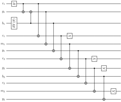
The next thing needed to obtain the results in Fig. 6 is a quantum circuit to prepare the ansatz containing the variational parameter. Based on the discussion surrounding Eq. 25, we anticipate that the physical ground state will have a contribution from the bare ground state as well as a triply degenerate contribution from three plaquette terms. Our variational parameter will be used to adjust the relative strengths of these two contributions. Our circuit is displayed in Fig. 7 and is responsible for the bottom panel of Fig. 6. This particular ansatz is quite simple, with two qubits at its core and extra CNOT gates adjusting the other qubits in a straightforward way. The circuit has been designed such that it requires minimal connectivity among the 12 qubits and is suitable, for example, to run on IBM’s heavy hex architecture without additional swap gates. The center panel of Fig. 6 uses the trial state obtained from the circuit in Fig. 8. The top panel of Fig. 6 uses a trial state that differs from Fig. 8 simply by appending a Pauli gate at the end of the circuit for each cyan, magenta and yellow qubit.
The final step to obtain the results in Fig. 6 is to measure the expectation value of each term in the Hamiltonian. Each term is a product of and gates. Expectation values involving only gates can be obtained directly from measurements of the state itself. Expectation values involving gates can be obtained by rotating into the computational basis with a pair of Hadamard gates, . Each data point in Fig. 6 comes from the linear combination of output from 4 separate runs of the circuit, one for , one for , one for , and one for .
References
- [1] C. Gattringer and C. B. Lang, “Quantum chromodynamics on the lattice,” Lect. Notes Phys. 788, 1-343 (2010) Springer, 2010, doi:10.1007/978-3-642-01850-3
- [2] F. Knechtli, M. Günther and M. Peardon, “Lattice Quantum Chromodynamics: Practical Essentials,” Springer, 2017, ISBN 978-94-024-0997-0, 978-94-024-0999-4 doi:10.1007/978-94-024-0999-4
- [3] N. Brambilla, S. Eidelman, C. Hanhart, A. Nefediev, C. P. Shen, C. E. Thomas, A. Vairo and C. Z. Yuan, “The states: experimental and theoretical status and perspectives,” Phys. Rept. 873, 1-154 (2020) doi:10.1016/j.physrep.2020.05.001 [arXiv:1907.07583 [hep-ex]].
- [4] P. Bicudo, “Tetraquarks and pentaquarks in lattice QCD with light and heavy quarks,” Phys. Rept. 1039, 1-49 (2023) doi:10.1016/j.physrep.2023.10.001 [arXiv:2212.07793 [hep-lat]].
- [5] T. Aoyama, N. Asmussen, M. Benayoun, J. Bijnens, T. Blum, M. Bruno, I. Caprini, C. M. Carloni Calame, M. Cè and G. Colangelo, et al. “The anomalous magnetic moment of the muon in the Standard Model,” Phys. Rept. 887, 1-166 (2020) doi:10.1016/j.physrep.2020.07.006 [arXiv:2006.04822 [hep-ph]].
- [6] K. Nagata, “Finite-density lattice QCD and sign problem: Current status and open problems,” Prog. Part. Nucl. Phys. 127, 103991 (2022) doi:10.1016/j.ppnp.2022.103991 [arXiv:2108.12423 [hep-lat]].
- [7] L. Funcke, T. Hartung, K. Jansen and S. Kühn, “Review on Quantum Computing for Lattice Field Theory,” PoS LATTICE2022, 228 (2023) doi:10.22323/1.430.0228 [arXiv:2302.00467 [hep-lat]].
- [8] C. W. Bauer, Z. Davoudi, A. B. Balantekin, T. Bhattacharya, M. Carena, W. A. de Jong, P. Draper, A. El-Khadra, N. Gemelke and M. Hanada, et al. “Quantum Simulation for High-Energy Physics,” PRX Quantum 4, no.2, 027001 (2023) doi:10.1103/PRXQuantum.4.027001 [arXiv:2204.03381 [quant-ph]].
- [9] A. Di Meglio, K. Jansen, I. Tavernelli, C. Alexandrou, S. Arunachalam, C. W. Bauer, K. Borras, S. Carrazza, A. Crippa and V. Croft, et al. “Quantum Computing for High-Energy Physics: State of the Art and Challenges. Summary of the QC4HEP Working Group,” [arXiv:2307.03236 [quant-ph]].
- [10] D. Banerjee, M. Bögli, M. Dalmonte, E. Rico, P. Stebler, U. J. Wiese and P. Zoller, “Atomic Quantum Simulation of U(N) and SU(N) Non-Abelian Lattice Gauge Theories,” Phys. Rev. Lett. 110, no.12, 125303 (2013) doi:10.1103/PhysRevLett.110.125303 [arXiv:1211.2242 [cond-mat.quant-gas]].
- [11] N. Klco, J. R. Stryker and M. J. Savage, “SU(2) non-Abelian gauge field theory in one dimension on digital quantum computers,” Phys. Rev. D 101, no.7, 074512 (2020) doi:10.1103/PhysRevD.101.074512 [arXiv:1908.06935 [quant-ph]].
- [12] A. Ciavarella, N. Klco and M. J. Savage, “Trailhead for quantum simulation of SU(3) Yang-Mills lattice gauge theory in the local multiplet basis,” Phys. Rev. D 103, no.9, 094501 (2021) doi:10.1103/PhysRevD.103.094501 [arXiv:2101.10227 [quant-ph]].
- [13] Y. Y. Atas, J. Zhang, R. Lewis, A. Jahanpour, J. F. Haase and C. A. Muschik, “SU(2) hadrons on a quantum computer via a variational approach,” Nature Commun. 12, no.1, 6499 (2021) doi:10.1038/s41467-021-26825-4 [arXiv:2102.08920 [quant-ph]].
- [14] S. A Rahman, R. Lewis, E. Mendicelli and S. Powell, “SU(2) lattice gauge theory on a quantum annealer,” Phys. Rev. D 104, no.3, 034501 (2021) doi:10.1103/PhysRevD.104.034501 [arXiv:2103.08661 [hep-lat]].
- [15] A. N. Ciavarella and I. A. Chernyshev, “Preparation of the SU(3) lattice Yang-Mills vacuum with variational quantum methods,” Phys. Rev. D 105, no.7, 074504 (2022) doi:10.1103/PhysRevD.105.074504 [arXiv:2112.09083 [quant-ph]].
- [16] M. Illa and M. J. Savage, “Basic elements for simulations of standard-model physics with quantum annealers: Multigrid and clock states,” Phys. Rev. A 106, no.5, 052605 (2022) doi:10.1103/PhysRevA.106.052605 [arXiv:2202.12340 [quant-ph]].
- [17] S. A Rahman, R. Lewis, E. Mendicelli and S. Powell, “Self-mitigating Trotter circuits for SU(2) lattice gauge theory on a quantum computer,” Phys. Rev. D 106, no.7, 074502 (2022) doi:10.1103/PhysRevD.106.074502 [arXiv:2205.09247 [hep-lat]].
- [18] R. C. Farrell, I. A. Chernyshev, S. J. M. Powell, N. A. Zemlevskiy, M. Illa and M. J. Savage, “Preparations for quantum simulations of quantum chromodynamics in 1+1 dimensions. I. Axial gauge,” Phys. Rev. D 107, no.5, 054512 (2023) doi:10.1103/PhysRevD.107.054512 [arXiv:2207.01731 [quant-ph]].
- [19] Y. Y. Atas, J. F. Haase, J. Zhang, V. Wei, S. M. L. Pfaendler, R. Lewis and C. A. Muschik, “Simulating one-dimensional quantum chromodynamics on a quantum computer: Real-time evolutions of tetra- and pentaquarks,” Phys. Rev. Res. 5, no.3, 033184 (2023) doi:10.1103/PhysRevResearch.5.033184 [arXiv:2207.03473 [quant-ph]].
- [20] R. C. Farrell, I. A. Chernyshev, S. J. M. Powell, N. A. Zemlevskiy, M. Illa and M. J. Savage, “Preparations for quantum simulations of quantum chromodynamics in 1+1 dimensions. II. Single-baryon -decay in real time,” Phys. Rev. D 107, no.5, 054513 (2023) doi:10.1103/PhysRevD.107.054513 [arXiv:2209.10781 [quant-ph]].
- [21] A. N. Ciavarella, “Quantum simulation of lattice QCD with improved Hamiltonians,” Phys. Rev. D 108, no.9, 094513 (2023) doi:10.1103/PhysRevD.108.094513 [arXiv:2307.05593 [hep-lat]].
- [22] J. B. Kogut and L. Susskind, “Hamiltonian Formulation of Wilson’s Lattice Gauge Theories,” Phys. Rev. D 11, 395-408 (1975) doi:10.1103/PhysRevD.11.395
- [23] S. Chandrasekharan and U. J. Wiese, “Quantum link models: A Discrete approach to gauge theories,” Nucl. Phys. B 492, 455-474 (1997) doi:10.1016/S0550-3213(97)00006-0 [arXiv:hep-lat/9609042 [hep-lat]].
- [24] M. Mathur, “Harmonic oscillator prepotentials in SU(2) lattice gauge theory,” J. Phys. A 38, 10015-10026 (2005) doi:10.1088/0305-4470/38/46/008 [arXiv:hep-lat/0403029 [hep-lat]].
- [25] T. Byrnes and Y. Yamamoto, “Simulating lattice gauge theories on a quantum computer,” Phys. Rev. A 73, 022328 (2006) doi:10.1103/PhysRevA.73.022328 [arXiv:quant-ph/0510027 [quant-ph]].
- [26] L. Tagliacozzo, A. Celi, P. Orland and M. Lewenstein, “Simulations of non-Abelian gauge theories with optical lattices,” Nature Commun. 4, 2615 (2013) doi:10.1038/ncomms3615 [arXiv:1211.2704 [cond-mat.quant-gas]].
- [27] E. Zohar, J. I. Cirac and B. Reznik, “Cold-Atom Quantum Simulator for SU(2) Yang-Mills Lattice Gauge Theory,” Phys. Rev. Lett. 110, no.12, 125304 (2013) doi:10.1103/PhysRevLett.110.125304 [arXiv:1211.2241 [quant-ph]].
- [28] E. Zohar, J. I. Cirac and B. Reznik, “Quantum simulations of gauge theories with ultracold atoms: local gauge invariance from angular momentum conservation,” Phys. Rev. A 88, 023617 (2013) doi:10.1103/PhysRevA.88.023617 [arXiv:1303.5040 [quant-ph]].
- [29] K. Stannigel, P. Hauke, D. Marcos, M. Hafezi, S. Diehl, M. Dalmonte and P. Zoller, “Constrained dynamics via the Zeno effect in quantum simulation: Implementing non-Abelian lattice gauge theories with cold atoms,” Phys. Rev. Lett. 112, no.12, 120406 (2014) doi:10.1103/PhysRevLett.112.120406 [arXiv:1308.0528 [quant-ph]].
- [30] R. Anishetty and I. Raychowdhury, “SU(2) lattice gauge theory: Local dynamics on nonintersecting electric flux loops,” Phys. Rev. D 90, no.11, 114503 (2014) doi:10.1103/PhysRevD.90.114503 [arXiv:1408.6331 [hep-lat]].
- [31] E. Zohar and M. Burrello, “Formulation of lattice gauge theories for quantum simulations,” Phys. Rev. D 91, no.5, 054506 (2015) doi:10.1103/PhysRevD.91.054506 [arXiv:1409.3085 [quant-ph]].
- [32] A. Mezzacapo, E. Rico, C. Sabín, I. L. Egusquiza, L. Lamata and E. Solano, “Non-Abelian Lattice Gauge Theories in Superconducting Circuits,” Phys. Rev. Lett. 115, no.24, 240502 (2015) doi:10.1103/PhysRevLett.115.240502 [arXiv:1505.04720 [quant-ph]].
- [33] P. Silvi, E. Rico, M. Dalmonte, F. Tschirsich and S. Montangero, “Finite-density phase diagram of a (1+1)-d non-abelian lattice gauge theory with tensor networks,” Quantum 1, 9 (2017) doi:10.22331/q-2017-04-25-9 [arXiv:1606.05510 [quant-ph]].
- [34] M. C. Bañuls, K. Cichy, J. I. Cirac, K. Jansen and S. Kühn, “Efficient basis formulation for 1+1 dimensional SU(2) lattice gauge theory: Spectral calculations with matrix product states,” Phys. Rev. X 7, no.4, 041046 (2017) doi:10.1103/PhysRevX.7.041046 [arXiv:1707.06434 [hep-lat]].
- [35] D. Banerjee, F. J. Jiang, T. Z. Olesen, P. Orland and U. J. Wiese, “From the quantum link model on the honeycomb lattice to the quantum dimer model on the kagomé lattice: Phase transition and fractionalized flux strings,” Phys. Rev. B 97, no.20, 205108 (2018) doi:10.1103/PhysRevB.97.205108 [arXiv:1712.08300 [cond-mat.str-el]].
- [36] I. Raychowdhury, “Low energy spectrum of SU(2) lattice gauge theory: An alternate proposal via loop formulation,” Eur. Phys. J. C 79, no.3, 235 (2019) doi:10.1140/epjc/s10052-019-6753-0 [arXiv:1804.01304 [hep-lat]].
- [37] P. Sala, T. Shi, S. Kühn, M. C. Bañuls, E. Demler and J. I. Cirac, “Variational study of U(1) and SU(2) lattice gauge theories with Gaussian states in 1+1 dimensions,” Phys. Rev. D 98, no.3, 034505 (2018) doi:10.1103/PhysRevD.98.034505 [arXiv:1805.05190 [hep-lat]].
- [38] I. Raychowdhury and J. R. Stryker, “Solving Gauss’s Law on Digital Quantum Computers with Loop-String-Hadron Digitization,” Phys. Rev. Res. 2, no.3, 033039 (2020) doi:10.1103/PhysRevResearch.2.033039 [arXiv:1812.07554 [hep-lat]].
- [39] E. Zohar and J. I. Cirac, “Removing Staggered Fermionic Matter in and Lattice Gauge Theories,” Phys. Rev. D 99, no.11, 114511 (2019) doi:10.1103/PhysRevD.99.114511 [arXiv:1905.00652 [quant-ph]].
- [40] I. Raychowdhury and J. R. Stryker, “Loop, string, and hadron dynamics in SU(2) Hamiltonian lattice gauge theories,” Phys. Rev. D 101, no.11, 114502 (2020) doi:10.1103/PhysRevD.101.114502 [arXiv:1912.06133 [hep-lat]].
- [41] Y. Ji et al. [NuQS], “Gluon Field Digitization via Group Space Decimation for Quantum Computers,” Phys. Rev. D 102, no.11, 114513 (2020) doi:10.1103/PhysRevD.102.114513 [arXiv:2005.14221 [hep-lat]].
- [42] V. Kasper, G. Juzeliunas, M. Lewenstein, F. Jendrzejewski and E. Zohar, “From the Jaynes–Cummings model to non-abelian gauge theories: a guided tour for the quantum engineer,” New J. Phys. 22, no.10, 103027 (2020) doi:10.1088/1367-2630/abb961 [arXiv:2006.01258 [quant-ph]].
- [43] Z. Davoudi, I. Raychowdhury and A. Shaw, “Search for efficient formulations for Hamiltonian simulation of non-Abelian lattice gauge theories,” Phys. Rev. D 104, no.7, 074505 (2021) doi:10.1103/PhysRevD.104.074505 [arXiv:2009.11802 [hep-lat]].
- [44] R. Dasgupta and I. Raychowdhury, “Cold-atom quantum simulator for string and hadron dynamics in non-Abelian lattice gauge theory,” Phys. Rev. A 105, no.2, 023322 (2022) doi:10.1103/PhysRevA.105.023322 [arXiv:2009.13969 [hep-lat]].
- [45] V. Kasper, T. V. Zache, F. Jendrzejewski, M. Lewenstein and E. Zohar, “Non-Abelian gauge invariance from dynamical decoupling,” Phys. Rev. D 107, no.1, 014506 (2023) doi:10.1103/PhysRevD.107.014506 [arXiv:2012.08620 [quant-ph]].
- [46] A. Kan, L. Funcke, S. Kühn, L. Dellantonio, J. Zhang, J. F. Haase, C. A. Muschik and K. Jansen, “Investigating a (3+1)D topological -term in the Hamiltonian formulation of lattice gauge theories for quantum and classical simulations,” Phys. Rev. D 104, no.3, 034504 (2021) doi:10.1103/PhysRevD.104.034504 [arXiv:2105.06019 [hep-lat]].
- [47] E. Zohar, “Quantum simulation of lattice gauge theories in more than one space dimension—requirements, challenges and methods,” Phil. Trans. A. Math. Phys. Eng. Sci. 380, no.2216, 20210069 (2021) doi:10.1098/rsta.2021.0069 [arXiv:2106.04609 [quant-ph]].
- [48] I. Raychowdhury, “Toward quantum simulating non-Abelian gauge theories,” Indian J. Phys. 95, no.8, 1681-1690 (2021) doi:10.1007/s12648-021-02170-6 [arXiv:2106.11475 [hep-lat]].
- [49] N. Klco, A. Roggero and M. J. Savage, “Standard model physics and the digital quantum revolution: thoughts about the interface,” Rept. Prog. Phys. 85, no.6, 064301 (2022) doi:10.1088/1361-6633/ac58a4 [arXiv:2107.04769 [quant-ph]].
- [50] D. González-Cuadra, T. V. Zache, J. Carrasco, B. Kraus and P. Zoller, “Hardware Efficient Quantum Simulation of Non-Abelian Gauge Theories with Qudits on Rydberg Platforms,” Phys. Rev. Lett. 129, no.16, 160501 (2022) doi:10.1103/PhysRevLett.129.160501 [arXiv:2203.15541 [quant-ph]].
- [51] M. Carena, E. J. Gustafson, H. Lamm, Y. Y. Li and W. Liu, “Gauge theory couplings on anisotropic lattices,” Phys. Rev. D 106, no.11, 114504 (2022) doi:10.1103/PhysRevD.106.114504 [arXiv:2208.10417 [hep-lat]].
- [52] X. Yao, “SU(2) gauge theory in 2+1 dimensions on a plaquette chain obeys the eigenstate thermalization hypothesis,” Phys. Rev. D 108, no.3, L031504 (2023) doi:10.1103/PhysRevD.108.L031504 [arXiv:2303.14264 [hep-lat]].
- [53] T. Jakobs, M. Garofalo, T. Hartung, K. Jansen, J. Ostmeyer, D. Rolfes, S. Romiti and C. Urbach, “Canonical momenta in digitized Su(2) lattice gauge theory: definition and free theory,” Eur. Phys. J. C 83, no.7, 669 (2023) doi:10.1140/epjc/s10052-023-11829-9 [arXiv:2304.02322 [hep-lat]].
- [54] T. V. Zache, D. González-Cuadra and P. Zoller, “Quantum and Classical Spin-Network Algorithms for q-Deformed Kogut-Susskind Gauge Theories,” Phys. Rev. Lett. 131, no.17, 171902 (2023) doi:10.1103/PhysRevLett.131.171902 [arXiv:2304.02527 [quant-ph]].
- [55] T. Hayata and Y. Hidaka, “String-net formulation of Hamiltonian lattice Yang-Mills theories and quantum many-body scars in a nonabelian gauge theory,” JHEP 09, 126 (2023) doi:10.1007/JHEP09(2023)126 [arXiv:2305.05950 [hep-lat]].
- [56] A. Chan, Z. Shi, L. Dellantonio, W. Dür and C. A. Muschik, “Hybrid variational quantum eigensolvers: merging computational models,” [arXiv:2305.19200 [quant-ph]].
- [57] C. W. Bauer, Z. Davoudi, N. Klco and M. J. Savage, “Quantum simulation of fundamental particles and forces,” Nature Rev. Phys. 5, no.7, 420-432 (2023) doi:10.1038/s42254-023-00599-8
- [58] B. Müller and X. Yao, “Simple Hamiltonian for quantum simulation of strongly coupled (2+1)D SU(2) lattice gauge theory on a honeycomb lattice,” Phys. Rev. D 108, no.9, 094505 (2023) doi:10.1103/PhysRevD.108.094505 [arXiv:2307.00045 [quant-ph]].
- [59] C. W. Bauer, I. D’Andrea, M. Freytsis and D. M. Grabowska, “A new basis for Hamiltonian SU(2) simulations,” [arXiv:2307.11829 [hep-ph]].
- [60] L. Ebner, B. Müller, A. Schäfer, C. Seidl and X. Yao, “Eigenstate Thermalization in 2+1 dimensional SU(2) Lattice Gauge Theory,” [arXiv:2308.16202 [hep-lat]].
- [61] E. J. Gustafson, H. Lamm and F. Lovelace, “Primitive Quantum Gates for an Discrete Subgroup: Binary Octahedral,” [arXiv:2312.10285 [hep-lat]].
- [62] S. Endo, Z. Cai, S. C. Benjamin and X. Yuan, “Hybrid Quantum-Classical Algorithms and Quantum Error Mitigation,” J. Phys. Soc. Jap. 90, no.3, 032001 (2021) doi:10.7566/JPSJ.90.032001 [arXiv:2011.01382 [quant-ph]].
- [63] F. Laves, “Zur Klassifikation der Silikate. Geometrische Untersuchungen möglicher Silicium-Sauerstoff- Verbände als Verknüpfungsmöglichkeiten regulärer Tetraeder,” Zeitschrift für Kristallographie, 82, no.1-6, 1 (1932) doi.org/10.1524/zkri.1932.82.1.1
- [64] H. S. M. Coxeter, “On Laves’ Graph Of Girth Ten,” Canadian Journal of Mathematics, 7, 18 (1955) doi:10.4153/CJM-1955-003-7
- [65] T. Sunada, “Crystals That Nature Might Miss Creating,” Notices of the American Mathematical Society, 55, no.2, 208 (2008). https://www.ams.org/notices/200802/tx080200208p.pdf
- [66] C. H. Séquin, “Intricate Isohedral Tilings of 3D Euclidean Space,” in Bridges Leeuwarden: Mathematics, Music, Art, Architecture, Culture, London: Tarquin Publications (2008), ISBN 9780966520194, http://archive.bridgesmathart.org/2008/bridges2008-139.html
- [67] J. H. Conway, H. Burgiel, C. Goodman-Strauss, “The symmetries of things,” A. K. Peters Ltd, Wellesley (2008), ISBN 9781568812205
- [68] R. Suizu and K. Awaga, “Line graph theory reveals hidden spin frustration and bond frustration in molecular crystals with strong isotropy,” J. Mater. Chem, C10, 1196 (2022).
- [69] Y. Chai, A. Crippa, K. Jansen, S. Kühn, V. R. Pascuzzi, F. Tacchino and I. Tavernelli, “Entanglement production from scattering of fermionic wave packets: a quantum computing approach,” [arXiv:2312.02272 [quant-ph]].
- [70] R. C. Farrell, M. Illa, A. N. Ciavarella and M. J. Savage, “Quantum Simulations of Hadron Dynamics in the Schwinger Model using 112 Qubits,” [arXiv:2401.08044 [quant-ph]].
- [71] M. Motta, C. Sun, A. T. K. Tan, M. J. O. Rourke, E. Ye, A. J. Minnich, F. G. S. L. Brandão and G. K. L. Chan, “Determining eigenstates and thermal states on a quantum computer using quantum imaginary time evolution,” Nature Phys. 16, 205-210 (2019) doi:10.1038/s41567-019-0704-4 [arXiv:1901.07653 [quant-ph]].
- [72] M. Urbanek, B. Nachman, V. R. Pascuzzi, A. He, C. W. Bauer and W. A. de Jong, “Mitigating depolarizing noise on quantum computers with noise-estimation circuits,” Phys. Rev. Lett. 127, no.27, 270502 (2021) doi:10.1103/PhysRevLett.127.270502 [arXiv:2103.08591 [quant-ph]].
- [73] C. Charles, E. J. Gustafson, E. Hardt, F. Herren, N. Hogan, H. Lamm, S. Starecheski, R. S. Van de Water and M. L. Wagman, “Simulating lattice gauge theory on a quantum computer,” [arXiv:2305.02361 [hep-lat]].
- [74] R. C. Farrell, M. Illa, A. N. Ciavarella and M. J. Savage, “Scalable Circuits for Preparing Ground States on Digital Quantum Computers: The Schwinger Model Vacuum on 100 Qubits,” [arXiv:2308.04481 [quant-ph]].
- [75] M. Asaduzzaman, R. G. Jha and B. Sambasivam, “A model of quantum gravity on a noisy quantum computer,” [arXiv:2311.17991 [quant-ph]].
- [76] L. Hidalgo and P. Draper, “Quantum Simulations for Strong-Field QED,” [arXiv:2311.18209 [hep-ph]].
- [77] O. Kiss, M. Grossi and A. Roggero, “Quantum error mitigation for Fourier moment computation,” [arXiv:2401.13048 [quant-ph]].
- [78] M. S. Anis et al., Qiskit: An open-source framework for quantum computing, doi:10.5281/zenodo.2573505 (2021).
- [79] https://vimeo.com/904585432
- [80] E. H. Moore, “On the reciprocal of the general algebraic matrix,” Bulletin of the American Mathematical Society. 26 (9): 394–395 (1920) doi:10.1090/S0002-9904-1920-03322-7
- [81] R. Penrose, “A Generalized inverse for matrices,” Proc. Cambridge Phil. Soc. 51, 406-413 (1955) doi:10.1017/S0305004100030401