Advancing Scanning Probe Microscopy Simulations: A Decade of Development in Probe-Particle Models

Abstract

The probe-particle model is an open-source package designed for simulation of scanning probe microscopy experiments, employing non-reactive, flexible tip apices (e.g., carbon monoxide, xenon, or hydrogen molecules) to achieve sub-molecular resolution. This abstract introduces the latest version of the probe-particle model, highlighting substantial advancements in accuracy, computational performance, and user-friendliness over previous versions. To demonstrate this we provide a comprehensive review of theories for simulating non-contact Atomic Force Microscopy (nc-AFM), spanning from the simple Lennard-Jones potential to the latest full density-based model. Implementation of these theories are systematically compared against ab initio calculated reference, showcasing their respective merits. All parts of the probe-particle model have undergone acceleration by 1-2 orders of magnitude through parallelization by OpenMP on CPU and OpenCL on GPU. The updated package includes an interactive graphical user interface (GUI) and seamless integration into the Python ecosystem via pip, facilitating advanced scripting and interoperability with other software. This adaptability positions the probe-particle model as an ideal tool for high-throughput applications, including the training of machine learning models for the automatic recovery of atomic structures from nc-AFM measurements. We envision significant potential for this application in future single-molecule analysis, synthesis, and advancements of surface science in general. Additionally, we discuss simulations of other sub-molecular scanning-probe imaging techniques, such as bond-resolved scanning tunneling microscopy and kelvin probe force microscopy, all built on the robust foundation of the probe-particle model. Altogether this demonstrates the broad impact of the model across diverse domains of surface science and molecular chemistry.

Keywords: Scanning Probe Microscopy, Atomic Force Microscopy Simulations, Bond-Resolved Atomic Force Microscopy

1 Introduction

The first Scanning Tunneling Microscopy (STM) and Atomic Force Microscopy (AFM) instruments, developed in 1981 [1] and 1986 [2], respectively, showcased the ability to visualize individual atoms of inorganic substrates. It took, however, another two decades of scanning probe microscopy (SPM) development to distinguish individual atoms inside organic molecules separated by a distance less than 1.5 Å, achieving sub-molecular resolution. This was accomplished by passivating the apex of the metallic tip with an inert molecule (carbon monoxide, hydrogen) or atom (Xe) [3, 4]. Due to their low reactivity, these tip apices reduce the possibility of damaging or manipulating the sample. Furthermore, the molecules are rather loosely attached to metallic tips, which makes them flexible. As a result, high-resolution scanning probe microscopy (HR-SPM) techniques need to function at low temperatures ($\leq 10~{}K$) to minimize thermal motion and prevent the passivating molecule or atom from desorbing from the tip.

The flexibility of the molecule attached to the tip allows it to deflect during the interaction with the sample. The tip apex deflection produces image distortions, which manifest themselves as either sharp lines at the ridges of the potential energy surface resembling bonds in HR-AFM [5] or a discontinuous contrast in the HR-STM images [5, 6]. A similar effect can be also found in Inelastic Electron Tunnelling Spectroscopy (IETS) [7].

The SPM has become a powerful tool for the chemical analysis and synthesis of individual organic molecules due to its ability to distinguish atoms at close distances, manipulate them, as well as to differentiate bond types. For instance, the HR-AFM with CO-decorated tip is sensitive to a bond order in aromatic systems [8], free electron pairs in highly electronegative atoms [9], the orbital configuration of transition metals in organometallic compounds [10].

The capabilities of SPM techniques made them invaluable tools not only in fundamental research (e.g. for the development of futuristic molecular and material nanotechnology [11]) but also in practical industrial applications. Currently, SPM helps in deciphering the chemical structures of individual molecules within complex mixtures, such as crude oil or decomposing and carbonized organic materials in the depth of oceans [12, 13, 14]. HR-SPM has been also extremely useful for the recognition of complex materials and their surfaces such as calcium carbonate and fluoride [15, 16], showing the HR-SPM general applicability over several scientific disciplines.

Due to single molecule resolution, HR-SPM techniques allows avoiding preparation of pure substances in macroscopic quantities which is required by other techniques for structural analysis such as X-ray or neutron diffraction. For example, the modern AFM machines, which can employ an automatic tip preparation [17], are restricted mainly by the sample preparation and are physically capable of scanning thousands of molecules per day for molecules deposited on metals, which could be great candidates for high-throughput usage of HR-SPM. However, the data interpretation, typically done by teams of human experts with the aid of atomistic simulations, proves to be a tedious and challenging process. This bottleneck hampers the broader adoption of SPM-based analytical methods beyond basic research.

The probe-particle model, first introduced nearly a decade ago [5], has become a widely used tool for simulating high-resolution AFM and STM images. The model enables the rationalization of experimentally observed SPM contrast and its attribution to chemical structure. From here on, we will focus on AFM simulations with the probe-particle model - PPAFM. PPAFM provides a good accuracy of simulated images at low computational cost. This enables rapid exploration of candidate molecular or surface structures and the exploration of suitable imaging parameters to match experimentally observed contrast to an a priori unknown geometry. Moreover, in recent years, PPAFM has emerged as a key driver of progress in the field of automatic interpretation of AFM data using machine-learned models [18, 19, 20], as well as for the construction of large datasets [21] of simulated AFM data. To the best of our knowledge, the PPAFM has served as the primary tool for generating training data for all machine-learned high-resolution AFM interpretation models published to date.

However, despite nearly a decade of development, the documentation surrounding PPAFM has been relatively scarce, leaving potential users largely unaware of its recent features, such as GPU acceleration, real-time Graphical User Interface (GUI), capability to conduct Kelvin Probe Force Microscopy (KPFM) simulations, and most importantly, implementations of advanced models of electrostatic and Pauli repulsion interactions based on ab initio calculated densities and potentials. Therefore, in this article, we aim to present the full spectrum of capabilities offered by the latest release of PPAFM and present it as a comprehensive toolbox for high-throughput simulations, encompassing not only high-resolution microscopy AFM but also STM, KPFM, IETS, and other related SPM techniques. The latest version of PPAFM provides an improved user interface and integration with various platforms. The installation process of PPAFM has become more streamlined. Last but not least, PPAFM is now accompanied by enhanced documentation. We believe that this enhancement will open the field of AFM simulation towards new users and new applications in molecular design, materials science, and surface science.

The paper is organized as follows. Section 2 describes the theoretical background of the PPAFM model in general as well as implemented models of tip-sample interaction in order of increasing accuracy. Section 3 discusses implemented models for the simulation of other SPM techniques such as STM, IETS and KPFM, which builds on top of the AFM model. Section 4 describes the code from the user’s perspective. The technical details concerning the implementation of the method are provided in section 5. Finally, the conclusion is given in section 6.

2 AFM simulation models

2.1 Tip description

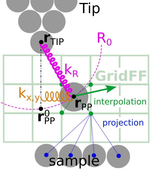
Figure 1: Schematics of forces acting on the flexible probe particle (PP) in PPAFM: The PP represents the very last atom of the non-reactive, flexible tip-apex (e.g. O atom of attached CO molecule), its position is denoted ${\vec{r}}_{PP}$. It is anchored to a rigid AFM tip by radial spring with high stiffness $k_{R}$ which keeps it in a certain distance $R_{0}$ from the anchor point $R_{TIP}$, and a lateral spring $k_{x,y}$ which tries to return to equilibrium position $R^{0}_{PP}$ under the tip. Besides the forces from the tip, also forces of the sample act on PP. These forces are calculated by interpolation of grid projected forcefield (GridFF). GridFF can be calculated by projection of atomic potentials (see Eq. 5, Eq. 6) or by convolution of grid projected densities (see Eq. 7, Eq. 8).

The original probe-particle model was based on a simple idea: simulating a non-reactive, flexible tip apex such as an attached CO molecule (or tip decoration like H₂, Xe [4], NTCDA [22] etc.) by modelling it as a single spherical particle attached to the end of an AFM tip by a lever with a bending spring. This spherical particle, which we call the probe particle (PP), represents the very last atom of the flexible tip apex (e.g. O atom in the CO-decorated tip). This simplistic approach is motivated by the fact that the short-range forces, that determine the measured sub-molecular contrast rapidly decay with distance and thus can be neglected for the other atoms of the tip-apex. This allows us to separate the forces from the tip (indexed with $T$) and forces from a sample (indexed with $S$) so that the overall force acting on the PP ($F^{PP}$) during its relaxation is evaluated as follows:

$$F^{PP}({\vec{r}}_{PP})=F^{T}({\vec{r}}_{PP})+F^{S}({\vec{r}}_{PP}),$$ (1)

The forces from the sample are discussed in greater detail in section 2.2.

The model for the forces from the tip is as follows:

$$F^{T}({\vec{r}}_{PP})=-k_{R}(|{\vec{d}}|-R_{0})({\vec{d}}/|{\vec{d}}|)-{\vec{k}_{x,y}}\odot({\vec{d}}-{\vec{d}}_{0})$$ (2)

Here, ${\vec{d}}={\vec{r}}_{PP}-{\vec{r}}_{TIP}$ is the displacement of the PP position ${\vec{r}}_{PP}$ with respect to the anchor point ${\vec{r}}_{TIP}$ to which the PP is attached (e.g. metallic tip apex to which the CO molecule it attached). $R_{0}=|\vec{d}_{0}|$ stands for the equilibrium distance from the anchor point and ${\vec{d}}_{0}={\vec{r}}^{0}_{PP}-{\vec{r}}_{TIP}$ is the equilibrium displacement of PP from the anchor point (which is typically $(0,0,R_{0})$ for a symmetric tip but may be deflected in x,y to simulate an asymmetric CO tip). Finally, $k_{R}$ is the radial stiffness constant and $\vec{k}_{x,y}=(k_{x},k_{y},0)$ sets the bending stiffness and $\odot$ denotes the component-wise product of vectors. This differs from the original model [5], which used the Lennard-Jones potential for the radial force, keeping the PP under the tip, while here we are using the strong spring force $k_{R}$, as this is a computationally faster and more stable solution. The lateral movement of the PP is still controlled by the lateral springs $k_{x}$ and $k_{y}$ as it is shown in Fig. 1(a). From our experience, CO tips are best reproduced using a lateral stiffness of 0.24-0.25 N/m [23].

The z-component of the short-range forces acting on the tip ($F_{z}^{tip}$) can then be calculated as the z-component of the radial spring force acting on the PP, $F_{z}^{tip}(\vec{r_{tip}})=-F^{T}_{R,z}$ at the fully relaxed position of the PP, as these forces balance each other out. $F_{z}^{tip}$ is then used for calculating the actually measured frequency shift $\Delta f$ using the formula derived by Giessibl [24]:

$$\Delta f^{tip}(\vec{r_{tip}})=-\frac{f_{0}}{2k}\frac{8}{\pi A^{2}}\int_{-A/2}^{A/2}\frac{zF_{z}^{tip}(\vec{r_{tip}}+\hat{A}z)}{\sqrt{A^{2}/4-z^{2}}}dz,$$ (3)

where $k$ is the stiffness and $f_{0}$ is the base oscillation frequency of the cantilever, $A$ is the peak-to-peak amplitude of the oscillation of the AFM tip and $\hat{A}$ is the normalized direction vector of the oscillation (typically in the z-direction).

2.2 Sample-tip interaction

The sample-tip interaction comprise of Pauli repulsion $F_{Pauli}$, van der Waals attraction (or London dispersion force) $F_{vdW}$, and electrostatic interaction $F_{el}$ between the PP and the sample:

$$F^{S}({\vec{r}}_{PP})=F_{Pauli}({\vec{r}}_{PP})+F_{vdW}({\vec{r}}_{PP})+F_{el}({\vec{r}}_{PP}).$$ (4)

The precision of the PPAFM simulation can be tuned by the level of theory describing these interactions.

In the following section, we cover the historical development of the different approximate models and their applicability. Despite the actual implementation relying on forces, for simplicity, we only discuss formulas to compute energy components. The respective formula for the force can be obtained as a derivative of the energy ${\vec{F}}({\vec{r}}_{PP})=-\nabla E({\vec{r}}_{PP})$.

2.2.1 Lennard-Jones

In the original (and the simplest) PPAFM model [5] the motion of the PP, ${\vec{r}}_{PP}$, is governed by a potential obtained as a sum of pair-wise Lennard-Jones potentials between the PP and all the atoms of the sample. The attractive and repulsive parts of Lennard-Jones potential simulate the attractive London dispersion and the Pauli repulsion respectively. The total potential is evaluated as follows:

$$E_{LJ}(\vec{r}_{PP})=e_{PP}\sum_{i}e_{i}\left[\left(\frac{R_{i,PP}}{|{\vec{r}}_{i}-{\vec{r}}_{PP}|}\right)^{12}-\left(\frac{R_{i,PP}}{|{\vec{r}}_{i}-{\vec{r}}_{PP}|}\right)^{6}\right]$$ (5)

Here the position of the sample atoms ${\vec{r}}_{i}$ are considered rigid (i.e. not movable), and traditional mixing rules such as $R_{i,PP}=R_{i}+R_{PP}$ and $e_{i,PP}=e_{i}e_{PP}$ are used to evaluate the equilibrium distance $R_{i,PP}$ and binding energy $e_{i,PP}$ of the $i$-th atom of the sample and the PP. The default parameters $e_{i},R_{i}$ are taken from the OPLS force field [25], but PPAFM also allows for a change of the element-based parameters in a user-provided parameter file.

2.2.2 Lennard-Jones with point charge electrostatics

Already in the same year, the model was modified to include the electrostatic interactions between the tip and the sample [7] to simulate image artifacts in IETS signal over electronegative nitrogen atoms in phthalocyanine.

Initially, the electrostatics was implemented as a sum of Coulomb potentials between classical point charges positioned at the centre of the PP ($q_{PP}$) and the sample atoms ($q_{i}$):

$$E_{el}({\vec{r}}_{PP})=k_{\mathrm{e}}q_{PP}\sum_{i}\frac{q_{i}}{|{\vec{r}}_{i}-{\vec{r}}_{PP}|},$$ (6)

where $k_{\mathrm{e}}$ is the Coulomb constant. Simultaneously with improvements of the physics captured by the PPAFM model, the assumption of a rigid sample allowed significant optimizations and acceleration of the simulations. Both the electrostatic and the LJ force field can be pre-calculated and stored on a real space grid, from which they are interpolated during the simulations. For a large sample containing hundreds of atoms this accelerates the simulations by 1-2 orders of magnitude (see sec. 5.1).

2.2.3 Lennard-Jones with density functional theory based electrostatics

A more accurate model of the electrostatics was developed in the same year using a grid-based real-space representation of electrostatic potential of the sample ($V_{S}$). $V_{S}$ is obtained as the Hartree potential from sample electronic structure calculation from density functional theory (DFT). The electrostatic potential acting on the PP with its charge density ($\rho_{PP}$) is obtained through a cross-correlation integral:

$$E_{el}({\vec{r}}_{PP})=\int_{\vec{r}}\rho_{PP}({\vec{r}}+{{\vec{r}}_{PP}})V_{S}(\vec{r})d\vec{r}.$$ (7)

The evaluation of this cross-correlation integral was accelerated using the Fast-Fourier Transform (FFT), relying on the convolution theorem (see sec. 5.1).

We found that the distortions in AFM images by electrostatic field to a large extent explain for example the over-enhanced bond-length contrast in fullerenes or other Kekule structures [8, 26] but also the repulsive contrast over triple bonds and free electron pairs [9]. Nevertheless, the charge required to reproduce experimental contrast with monopole charge distribution was unrealistically high (0.2-0.4e).

In further applications of this model for mapping of the electrostatic force field of a TOAT molecule and a PTCDA layer [27], and for imaging of H₂O clusters on sodium chloride [28, 29], we concluded that a quadrupolar charge distribution on the PP is a better model for real charge distribution of a CO molecule and therefore better reproduces the observed image contrast. This was further supported by a DFT calculation of the CO-tip density [28] and more detailed analysis conducted by other authors [30].

While point-charge electrostatics proved useful for quick and easy model calculations independent of ab initio inputs, which were often conducted by external experimental groups through a web interface [31], DFT-based electrostatics of the sample was, nevertheless, found necessary to properly simulate intricate image effects, such as those arising from free electron pairs and triple bonds. For the CO tip the quadrupole moment can vary in between -0.025 to -0.15 $e\times\AA{}^{2}$, depending on the experiment [32, 18, 27].

A minor disadvantage of the cross-correlation-based approach (see sec. 5.1) is the assumption that the PP moves without rotation (i.e., bending of the CO tip is simulated by shifting rather than rotating the CO molecule). This assumption is accurate for models considering spherically symmetric PPs (e.g., monopole electrostatics, spherical Lennard-Jones potential). However, for models considering quadrupolar electrostatics, or ab initio electron density of the tip, the assumption of the irrotational PP may pose a problem. According to our experience with the complex-tip model [33] and comparison of our PPAFM model against the direct integration model by Ellner at al. [30] the differences caused by the multipole rotation are minor. This can be understood from the fact that bending angles are rather small at tip-sample distance relevant for high-resolution imaging experiments, and the bending is most significant at the close range where the interaction is dominated by the Pauli rather than electrostatic interaction.

2.2.4 Full density-based model

Pauli repulsion modeled by the repulsive part $(1/r^{12})$ of the spherically symmetric Lennard-Jones potential cannot reproduce delicate effects emerging from rearrangements of the electron density in the sample which are often visible using HR-AFM techniques [8, 9, 10]. Some of these limitations can be mitigated by modification of the Lennard-Jones parameters of individual atoms (especially van der Waals radius) to match the iso-surface of electron density obtained from a DFT calculation [10]. This approach allows to distinguish between different occupations of the atomic orbitals for atoms of the same element and it was also successfully used for calculations of ionic materials, such as calcite or calcium fluoride [16, 15]. Nevertheless, such approach is still limited by the spherical symmetry of the Lennard-Jones potential, therefore it cannot fully recover non-spherical effects such as free-electron pairs and variation of density in covalent bonds.

In order to addresses these limitations, Ellner et al. [34] introduced an improved model called the full density-based model (FDBM), where both the Pauli repulsion and electrostatics are calculated directly from electron density obtained from DFT. While electrostatics is still calculated using Eq. 7, the Pauli repulsion is newly calculated by the integral of the product of the tip and the sample charge densities scaled by a fitting constant $A$. Eventually the product is raised to exponent $\beta$ (although $\beta$ is typically close to one):

$$E_{Pauli}({\vec{r}}_{PP})=A\int_{\vec{r}}\left[\rho_{PP}({\vec{r}}+{{\vec{r}}_{PP}})\rho_{S}(\vec{r}))\right]^{\beta}d\vec{r}$$ (8)

The magnitude of the repulsion is significantly more sensitive to the exponent $\beta$ than the multiplicative factor $A$. Even a change of only $0.1$ in $\beta$ results in a significant change in the observed contrast, higher values typically resulting in reduced sharpness. However, if the scanning distance and $A$ are adjusted along with $\beta$, similar-looking contrast can be observed with multiple distinct combinations of the parameters. Since this formula can be interpreted as a cross-correlation similarly to Eq. 7, we can also utilize FFT for acceleration allowing us to conduct FDBM simulations in $\sim$1 minute on single CPU and fraction of a second using contemporary GPUs (see sec. 5.1).

The resulting model, combined with an appropriate dispersion interaction model (previously modeled by the attractive part of the Lennard-Jones potential), and properly fitted, could remarkably reproduce experimentally measured images of rigid molecules. Particularly, it better captures the free electron pairs (e.g., oxygen and nitrogen heteroatoms) and Kekule structures (e.g., triple bonds), which were previously only emulated through the repulsive electrostatic field in the original Lennard-Jones-based model sometimes using unrealistically high tip charge [26]. Now FDBM also accounts for Pauli repulsion, capturing the electron hardness of free electron pairs on oxygen and nitrogen atoms.

The dispersion interaction model typically used with the FDBM is the Grimme DFT-D3 [35] dispersion correction, which we have also recently implemented in PPAFM, in particular in the Becke-Johnson damping form [36]. One notable aspect of the DFT-D3 correction is that the interaction coefficients for each atom depend on their chemical environment, based on proximity, in order to account for the changing polarizability due to bonding. In principle the distance calculations to determine the bonding configuration would also include the PP. However, since the PP is supposed to be chemically inert, we choose to exclude the PP from this calculation, which allows the interaction coefficients in the sample to be calculated independent of the PP position, significantly speeding up the calculation.

The DFT-D3 energy also has parameters that are adjusted for particular DFT functionals - namely s₆, s₈, a₁, and a₂ [35]. So far there has not been any extensive study on the effect of these parameters on PPAFM simulations and thus we recommend to stick to the parameters connect with the DFT functional used for calculation of the FDBM models input. PPAFM provides here predefined parameter values for many of commonly used DFT functionals.

2.2.5 Comparison of AFM simulation models

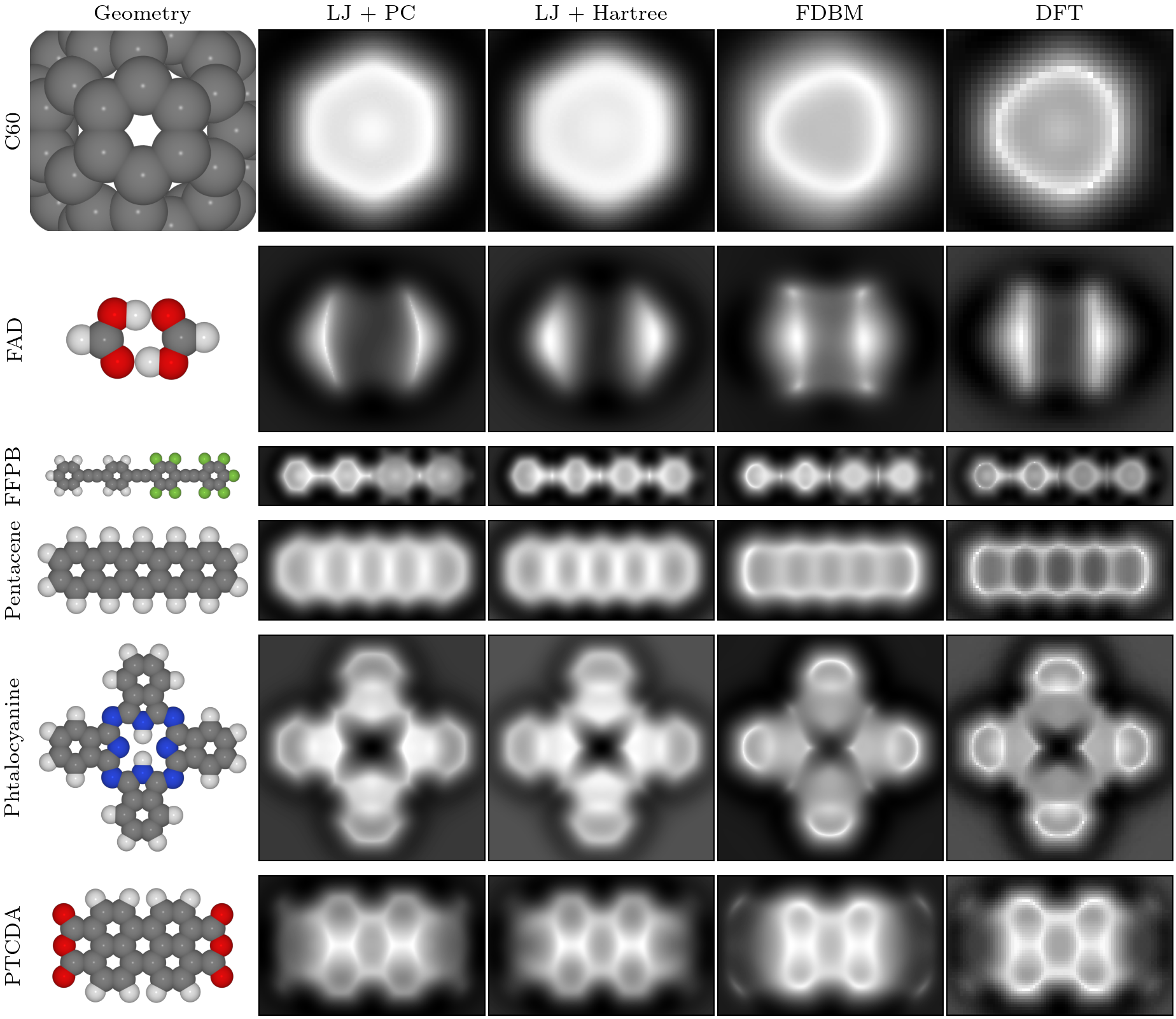
Figure 2: Comparison of PPAFM simulations with different models of tip-sample interaction. The columns depict different models. Starting from the left, they are Lennard-Jones + point charges (LJ+PC), Lennard-Jones + Hartree (LJ+Hartree), Full density based model (FDBM), and a DFT simulation used as a reference, where tip-sample interaction at each pixel was calculated as an independent relaxation of the tip using the CP2K program. For the Lennard-Jones based simulation model (both with point-charge and Hartree potential) we used a quadrupole charge distributions on the tip with the quadrupole moment $-0.05\,e\times\AA{}^{2}$. For the point-charge simulations we used Mulliken charges reported by FHI-aims [37]. For FDBM model we set the multiplicative factor $A=1.2$ and exponent $\beta=1.2$ (see Eq. 8) which provided best overall match to DFT for all the molecules.

In order to illustrate strengths and weaknesses of each tip-sample interaction model we plot in Fig. 2 results calculated for a representative selection of molecules. We compare our PPAFM simulations against a DFT reference calculations performed via CP2K [38] with PBE exchange-correlation functional and Grimme DFT-D3 [35] used for the van der Waals correction. Each of the selected molecules represent some characteristic chemical moieties manifested as characteristic features in AFM and was previously discussed in HR-AFM related literature. To make the comparison consistent we choose same simulation parameters for each molecule, despite this choice may be not optimal to represent DFT reference or experimentally observed contrast. This means that for FDBM model we set the multiplicative factor $A=12$ and exponent $\beta=1.2$ (see Eq. 8), which provided best overall match to DFT for all the molecules. We found that the best match is visible if we offset z-distance by $-0.2\,\AA$ between the DFT and the PPAFM simulations in order to get a roughly matching level of sharpness in the observed contrast. In the FDBM simulation the electrostatics used a DFT-calculated charge density on the CO-tip. For the Lennard-Jones based simulation model (both with point-charge and Hartree potential) the we used quadrupole charge distributions on the tip with quadrupole moment $-0.05\,e\times\AA{}^{2}$. For point charges simulations we used Mulliken charges reported by FHI-aims [37].

C60 Fullerene was studied as an example of bond order discrimination [8]. Difference in the apparent bond length, as well as the ovaloid shape of electron cloud is very well reproduced by the FDBM model. To some degree the difference in apparent bond length can be reproduced also with the LJ+Hartree model, nevertheless unrealistically high charge of the tip is needed to reproduce experimental (or DFT calculated) contrast [26].

FAD (Formic acid dimer)) represents carboxylic groups which often dimerize in self-assembled structures studied by AFM [9, 39]. The FDBM again provides contrast most similar to DFT data, including bright spots above oxygen atoms. This is due to ability of FDBM to reflect localized electron pairs in Pauli repulsion. Nevertheless these bright spots are visible also in LJ+PC and LJ+Hartree simulations at higher tip-sample separation where electrostatic forces dominate [9].

FFPB molecule (4-(4-(2,3,4,5,6- pentafluorophenylethynyl)- 2,3,5,6- tetrafluorophenylethynyl) phenylethynylbenzene) was studied to see the effect of electron depletion on the AFM contrast in a benzene ring ($\pi$-hole), caused by the electron withdrawing substituents (fluorines) [40, 41]. In DFT simulations this is visible as darker contrast over fluorinated rings, which can be attributed to a faster decay of the electron density [42] (due to deeper electrostatic potential and lower work function) and by electrostatic attraction between the ($\pi$-hole) and free electron pair of CO tip. Surprisingly, this effect is best reproduced by LJ+PC model, which used Mulliken charges obtained from DFT calculation. Another characteristic feature clearly visible in this molecule is the triple bond rendered as bright line perpendicular to the bond. This effect is caused by the toroidal shape of the $\pi$-electron cloud around the triple bond [43, 9], which produce a quadrupolar field both in electrostatics and Pauli repulsion. FDBM again reproduce this feature best thanks to incorporation of proper aspherical Pauli repulsion, while the Lennard-Jones potential is composed of spherical potentials around each atom and therefore cannot reproduce this feature. Nevertheless both LJ+PC and LJ+Hartree can reproduce the electrostatic contribution of this repulsive feature.

Pentacene molecule was one of the first molecules for which bond-resolved AFM images were measured [3]. Beside the five hexagonal rings the experiment and DFT simulations shows clearly increased repulsion over the ends of the aromatic system. This effect is to a large degree caused by higher attractive van der Waals background in the center as was explained in original paper [3]. Nevertheless our simulation done at closer tip-sample separation shows, that the effect is pronounced even at distance where van der Waals contribution is negligible. This is reproduced by FDBM but not with LJ-based models. Without detailed analysis we can only speculate that this is because tails of occupied frontier molecular orbitals (HOMO, HOMO-1 etc.) which contribute most to Pauli repulsion are more supressed in the center due to presence of nodes. Similar effect we often see in high resolution STM experiments also for other molecules. All models including FDBM and LJ-based models reproduce very well the distortion (elongation) of the rings perpendicular to the molecule axis, which is caused by deflection of the probe mostly due to lateral gradient of van der Waals potential (with a slight contribution from electrostatics), as was discussed previously [44, 27].

Phtalocyanine molecule was widely studied in the SPM community [45, 46, 10, 47] due its great potential for molecular electronics and catalysis, and for biological importance of porphirine derivatives. The main features which can be seen in HR-AFM experiments and which are perfectly reproduced by DFT simulations are: (i) The bright peripheral benzene rings contrasting against the darker porphirine center, and (ii) sharp pointy corners of imine nitrogens. Both of these features are nicely reproduced by FDBM, which properly accounts for the Pauli repulsion affected by slower decay of electron clouds in benzene rings (with respect to the porphirine center), as well as Pauli repulsion of the free electron pairs of these nitrogens. The LJ-based model incorrectly renders the pentagonal rings brighter. This is a simple effect of higher concentration of repulsive atoms in the pentagon ring in contrast to the hexagon. This failure of the LJ model to reproduce this effect is understandable, as it cannot account for rate of decay of tails of electron density. Nevertheless, the pointyness of the nitrogen groups is rather well reproduced mostly due to the significant role of the electrostatic forces which cause apparent shrinking of these areas as previously discussed [7].

PTCDA (Perylene carboxylic anhydride) is perhaps the most studied molecule in the SPM community [4, 42, 5, 27, 48], mostly due to experimental convenience and formation of well ordered self-assembled monolayers. The experiments as well as DFT simulations show the central perylene system considerably brighter than the peripheral anhydride groups. This is more-or-less reproduced by all models, although FDBM model excels in this aspect, as it reflects higher Pauli repulsion due to the longer extent of the electron cloud over the perylene system [42]. All models properly describe apparent enlargement of the anhydride groups and shrinking of the perylene group caused by electrostatic forces [27]. In addition, the DFT simulation shows bright repulsive features over the carbonyl oxygens, which are again best reproduced by FDBM model.

Despite generally superior accuracy of the FDBM approach, the PPAFM code allow users to choose from various simulation models (Lennard-Jones, Morse, point charges, model charge density integration, FDBM) the one which offers an optimal compromise between accuracy and simplicity for their particular application. Such a choice should not be motivated by computational cost of AFM simulations, as our efficient GPU implementation allows interactive simulations even on the FDBM level.

Nevertheless, the simpler models (e.g., Lennard-Jones + point charges) limit reliance on DFT data (i.e. charge density and Hartree potential are not required). This makes those simple models very convenient for fast screening over various modeled sample geometries or creation of databases for machine learning approaches. The dependence of the DFT electrostatics and FDBM method on DFT calculations (at least thousand times slower) and large amount of volumetric data are making this method less attractive for fast high-throughput simulation scenarios. For rapid training of AFM recognition models, we recommend pre-training the model on the data obtained from simple Lennard-Jones and point-charge-based simulations, with the refinement step performed on fewer examples generated by the FDBM (similar approach was used in [20]).

Notice that Lennard-Jones simulations presented in 2 were done using default Lennard-Jones parameters which depend only on chemical elements, not on more detailed atomic types (i.e. we do not distinguish different sub-types of carbon like sp¹, sp², aromatic, carboxylic etc.). With more careful selection of atomic types and of Lennard-Jones parameters (particularly the atomic radius) even the simple Lennard-Jones model can simulate the different extent of electron clouds and bring LJ-PC model closer to AFM experiments without the need of DFT inputs [10, 16]. Although FDBM model does not depend on such detailed choice of atomic types (assuming van der Waals D3 parameters are given, and has minor effect on resulting contrast), it still depend on choice of the two global parameters (scaling factors $A$ and exponent $\beta$ in Eq. 8). Optimal choice of these two parameters is still under debate, and may be system dependent.

3 Other PP-SPM simulation modes

AFM simulation models discussed in previous section are the central part of probe-particle simulations as they determine forces acting on PP and therefore also its relaxation (deflection). This deflection then modify the measured contrast of other signals (such as STM [5, 6] and IETS [7]), typically by sharpening or introducing discontinuities to the contrast. Beside this other forces can emerge in the junction between tip and sample e.g. due to polarization of the PP or the molecule under study by external electric field. These microscopic contributions of the polarization force which is responsible for sub-molecular contrast in Kelvin probe force microscopy (KPFM) can be also simulated within the PPAFM framework. The following section discusses simulation techniques of all these different techniques which are built on top of the PPAFM core.

3.1 Kelvin probe force microscopy

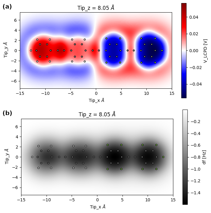
Figure 3: (a) LCPD map taken over the FFPB molecule, simulated using the KPFM functionality of PPAFM. (b) AFM image for the same tip distance as in the LCPD map. Images in both panels are overlaid with atomic structure of the FFPB molecule. The Tip_z = $8.05$ Å distance quoted as the height of the scanning plane position was measured between the molecular plane and the anchor pivot (metallic apex) of the tip. The tip distance $z_{\mathrm{tip}}=4.05$ Å used to scale the electric field induced by the voltage between the tip and the molecule was smaller by $R_{0}=4.00$ Å. A CO-tip model with the static quadrupole moment of $-0.05$ $e\times\AA{}^{2}$ and default electric polarizability was used. The capacitance of the metallic part of the tip was modeled with a sphere of the $R_{\mathrm{tip}}=40$ nm radius.

Traditionally, KPFM experiments measured the electrostatic forces between tip and sample due to external electric potentials and differences between the work functions of the two materials. In this process the tip and the sample can be seen as the plates of a capacitor. The force between such plates depends quadratically on the potential difference between the tip and the sample $V$ and linearly on the gradient of the effective capacitance $C({\vec{r}}_{tip})$ with respect to the position of the tip.

$${\vec{F}}({\vec{r}}_{tip})=\frac{V^{2}}{2}\nabla C({\vec{r}}_{tip}).$$ (9)

Although KPFM experiments were originally intended to measure mesoscopic features such as the work function of the studied materials and long-range charge domains, the development of atomically precise SPM techniques had allowed to achieve sub-molecular KPFM contrast, corresponding to variations of the charge distribution and polarizability within individual organic molecules [46, 49, 40, 50]. Nevertheless, the quantitative relation between the measured quantities and the electronic structure of the molecules was under debate. We developed a Kelvin Probe Force Microscopy modality into the PPAFM code in order to put these relations on quantitative ground and provide a straightforward tool for the simulation of these phenomena.

In this implementation, the bias dependence of both the charge density of the probe and the electrostatic potential of the sample is introduced in Eq. 7, to study its effect on the force ${\vec{F}}_{PP}({\vec{r}}_{tip})$ and the corresponding frequency shift $\Delta f$. As has been shown in our previous publications [51, 41], the sub-molecular variation of $\Delta f(V)$ originates mostly from the intrinsic charges within the tip or the sample that interact with bias-induced electric polarization of the opposite electrode. The output of the KPFM mode can be represented as a map of (apparent) local contact potential difference (LCPD or $V_{\mathrm{LCPD}}$), which corresponds to the bias voltage at which the maximum of the (approximately) parabolic $\Delta f(V)$ dependence lies.

Currently, the KPFM functionality is implemented in the PPAFM package in two variants. In the first version, the changes in the charge densities of the tip and sample due to the application of an external field in the z-direction must be provided as inputs from external DFT calculations. In the second version, analytically generated tip polarizations, fitted to the DFT calculated ones, are provided for user convenience. For a more detailed description of the usage of the KPFM module and the theoretical basis of the model, please refer to the code manual and the supplementary information of [51].

As an example of a KPFM simulation, Fig. 3a shows the LCPD map over the FFPB molecule. The LCPD is affected by the local electric charges on the molecule: positive charge under the tip tends to shift the LCPD towards more negative values, negative charge towards more positive values. The resulting figure clearly shows the polarization within the molecule. The two positive-charged (electron-depleted) benzene rings in the right-hand-side half of the molecule are surrounded by negative charge of the fluorine atoms, while the two electron-rich benzene rings in the left-hand-side half are surrounded by more positive hydrogen atoms. Notice that the simulated contrast is consistend with experimentally measured KPFM pictures from literature [40]. KPFM experiments usually need to be performed with larger tip–sample distance as compared to HR-AFM; we have considered this in our choice of tip distance for the simulation depicted in Fig. 3. The blurred AFM image in shown in Fig. 3b, dominated by attractive tip-sample interactions, is simulated at the same tip-sample distance as the KPFM image in Fig. 3b. Compare this with the HR-AFM of FFPB in Fig. 2 simulated at much closer tip-sample separation.

3.2 Bond-resolved STM

Despite the fact that the bond-resolved STM technique preceded sub-molecular resolution in the AFM [4], this technique received less attention in scientific community because the interpretation of the measured signal was unclear. In order to put the interpretation of these techniques on more quantitative grounds, and provide a straightforward simulation tool, we developed PPSTM [6, 52] which builds on top of PPAFM. The PPSTM code can be used as a standalone STM simulation package (independent of PPAFM) to simulate normal STM with rigid (e.g. metallic) tip. It is based on Chen’s rules [53] approximation of Bardeen tunneling theory to evaluate tunneling current between the tip and sample.

Nevertheless, the real strength of the PPSTM code is in its capability to calculate high-resolution (i.e. bond-resolved) STM images obtained with flexible tip-apices (e.g. CO, Xe, H₂) on organic molecules. In this application PPSTM is combined with the PPAFM code for pre-calculating the PP positions ${\vec{r}}_{PP}$ for each position of the tip ${\vec{r}}_{tip}$ during the scanning. This essentially just shifts the position of the orbitals located on the PP involved in the Chen’s tunneling formulas, as is illustrated in Fig. 4(a), which distorts the resulting image and gives rise to the characteristic sharp contrast in the high-resolution STM images as was described in [5, 6]. Bond-resolved imaging and STM simulations can be especially beneficial for STM machines without AFM possibilities, since STM measurements are tipically experimentally simpler than AFM. This was used for example for study of carbon nanoribbons and other graphitic structures [54, 55].

The main drawback of this approach is the added complexity of the interpretation and theoretical rationalization of the measured STM signal, which depends both on geometrical relaxation of probe-particle as well as on the electronic structure of the sample, and the tip, as is illustrated in Fig. 4(b) and (c). The interpretation is even more complicated (in comparison to AFM) when the electronic structure of the molecule is modified by interaction with interface state of the substrate, especially on metallic substrates [6]. Precise DFT calculations and use of hybrid functionals is often required to reproduce these delicate interface states in order to achieve agreement with experiment.

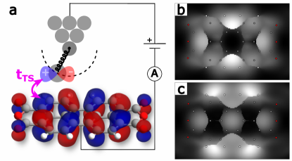
Figure 4: Schematics of PPSTM with example of PTCDA. (a) PPSTM calculates the electron tunneling rate $T_{TS}$ between the molecular orbitals of the sample and the tip using Chen’s rules [53]. The orbitals of the tip are modeled by atomic orbitals, like $s,p_{z},p_{x}$ (on the image) and $p_{y}$, positioned at the probe particle. This is done for the PP positions previously relaxed by PPAFM in order to account for the displacement of e.g. a CO molecule caused by the interaction with the sample. (b,c) Examples of a simulated PPSTM of the PTCDA molecule image using the dIdV mode. The model electronic structure of the tip was chosen to be $13\%$ of $s$ PP orbital and $87\%$ of $p_{x}$ and $p_{y}$ orbitals. This configuration best reproduced experimentally observed contrast measured with CO-tip in the previous publications (e.g. [32]). (b) at the sample bias corresponding to the HOMO orbital energy. (c) at the sample bias corresponding to the LUMO orbital energy. Please note that in the experiment the STM contrast can be affected by interaction of molecular orbitals with the interface states the substrate, forming a delicate electronic structure.

3.3 Inelastic scanning tunneling microscopy

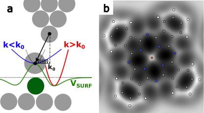
Figure 5: PP-IETS with example of Iron Phtalocyanine (FePc). (a) Schematic illustration of the PP-IETS imaging mechanism. The stiffness of the lateral CO vibration ($k_{0}$) is modified by curvature of the tip-sample interaction potential $V_{surf}$. The stiffness as well as the associated vibration frequency is increased at the position of a convex $V_{surf}$ and decreased at position of a concave potential (e.g. above atoms and bonds). Due to broadening of peaks measured in IETS spectroscopy, this softening of the modes above atoms and bonds allows detecting higher amplitude of inelastic tunneling signal originating from lateral CO vibration below the base energy $\epsilon_{0}$ associated with the base stiffness $k_{0}$, as was done by the Ho group [56]. For a more detailed explanation please see [7, 32]. (b) Example of an IETS map calculated by PPAFM on the iron phtalocyanine (FePc) molecule using just a Lennard-Jones force-field. Notice that in this particular simulation neither the distortions caused by electrostatics as discussed in [7] nor the modulation of the tunneling signal by orbital symmetry discussed in [32] are present.

Another method to achieve sub-molecular resolution, very close to the HR-AFM contrast, was demonstrated by the Ho group with inelastic STM [56]; however, without explanation of its mechanism. Already in the same year we were able to explain and simulate the observed contrast with the new IETS module added to our PPAFM package [7]. This module calculates the change of the stiffness (resp. vibration frequency) of lateral vibration modes of the CO molecule attached to AFM tip due to its interaction with the sample (see Fig. 5a). In repulsive regime the ridge-lines in tip-sample interaction potential (e.g. over the bonds between atoms in the sample) introduce negative curvature to the total potential in which the CO molecule vibrates. This effectively decreases the stiffness and vibration frequency of the relevant vibration mode, therefore shifting the inelastic tunneling peaks to lower energy. The technique discovered by Ho group basically maps the stiffness of the CO vibration as the tip moves over the sample. This effect is visible in simulated map shown in Fig. 5b, where bright contrast above the atoms and bonds correspond to increased inelastic tunnelling signal at energy (i.e. bias voltage set-point) below the base energy of latheral CO vibration mode. The amplitude of the peak is related to shift of the peak energy when considering e.g. Gaussian broadening as explained in [7].

Later we were able to improve this technique by considering the modulation of the observed signal by the variation of the tunneling current which depends on the orbital symmetry [32]. More precisely, the inelastic signal is modulated by electron-phonon coupling between the tunneling (calculated by Chen’s rules as in section 3.2) and the lateral vibration mode. Spatial dependence of this electron-phonon coupling is therefore proportional to the lateral derivative of the tunneling signal (i.e. derivative along the vibration vectors), as described in detail in [32].

4 PPAFM from the user perspective

4.1 Installation

The default way to install the PPAFM code is through the pip installer for Python packages. This can be achieved by running

⬇

pip install ppafm

on the command line. This installs the package from the Python Package Index (PyPI), which contains pre-compiled distributions of the PPAFM code for several operating systems. If the binary files for your environment do not exist, the ”pip” tool will attempt to compile them upon download. Additionally, pip installs all the necessary Python dependencies. Some non-Python GPU dependencies, however, might be installed separately from appropriate OpenCL-capable GPU drivers and related libraries. For more experienced users and developers we provide alternative ways of installing and running the code. The most up-to-date installation instructions can always be found in the repository [57]. They include installation in a dedicated Conda environment, Docker container, building from the source code, and others.

4.2 Command-line user interface

The command-line interface (CLI) of the PPAFM code provides users with access to the full capabilities of the package. This is an alternative to the graphical user interface discussed in the following section. The CLI interface allows to run simulations on supercomputers, cloud computers, and other computational resources without a graphical interface. Also, the CLI interface is used for high-throughput simulations when run by a workflow manager.

Once the PPAFM package is installed user gets access to a variety of tools to compute force fields, relax the probe particle, and plot the results. Below is an example of launching PPAFM to compute the Lennard-Jones force field:

⬇

ppafm-generate-ljff -i structure.xyz

In the example above we specify an XYZ file with an input structure. Additionally, the user can create a ”params.ini” file containing more fine-tuning settings of the simulation. If the file is present in the folder, the code will pick it up automatically. The PPAFM repository [57] contains detailed instructions on how to use PPAFM throught the CLI.

4.3 Graphical user interface

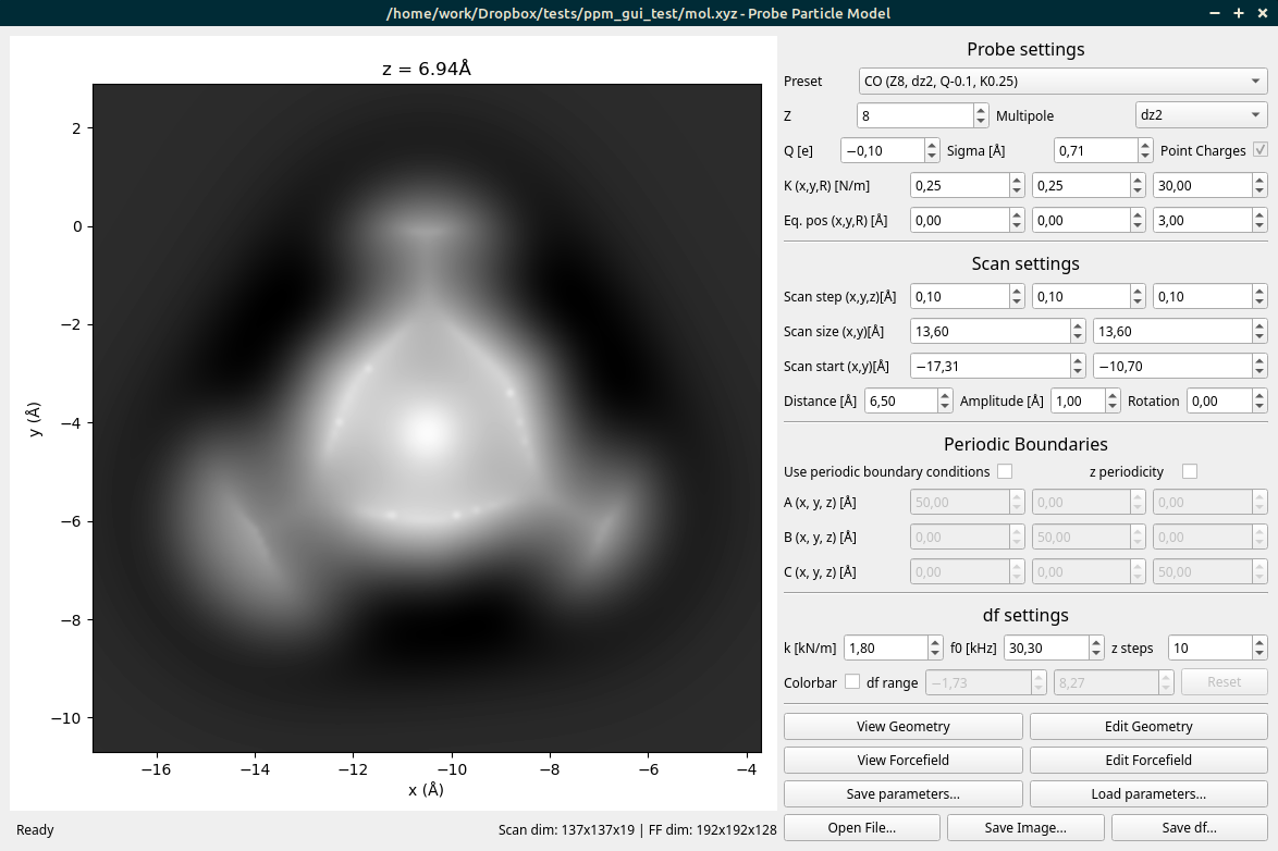
Figure 6: Interactive GUI for GPU-accelerated PPAFM simulations. The user can interactively modify imaging parameters by using input boxes or a mouse-wheel, and image contrast is updated automatically.

The latest GPU-accelerated version of the PPAFM code is so fast that interacting with the user solely through scripts or a bash terminal becomes a significant bottleneck. Simulations of a full stack of AFM images with typical resolutions of 200x200x20 pixels take $\small\sim\>\!$$0.1\text{\,}\mathrm{s}$ on a typical desktop computer equipped with a dedicated GPU. For this reason, we have developed a simple graphical user interface (GUI) (see Fig. 6) that enables users to quickly explore simulation results obtained with different inputs. Users can vary parameters such as the bending stiffness of the CO tip, oscillation amplitude of the AFM cantilever, effective charge of the tip, or parameters of the FDBM model, and immediately visualize the results for comparison with experimental references. This approach is particularly useful for new users who are trying to familiarize themselves with the code and gain intuition about how various imaging parameters can affect measured AFM contrast. This exploration can be also useful to the experimentalist who wishes to gain an idea of what to expect from the images from a real HR-AFM machine. Another application is manually finding the set of parameters that most closely resembles a specific set of reference AFM images obtained with a particular setup. This can be used, for example, in the refinement of training data for machine-learned models of automatic image interpretation.

4.4 Integration with other software

In order to fully exploit the computational efficiency of the PPAFM code (especially in GPU-accelerated version) for machine-learning and other high-throughput applications, we provide a Python application programming interface (API) which allows for seamless integration with other Python-based software. In particular, this API was used to rapidly generate training data for a machine-learning application for automated AFM image interpretation [18].

The Python API is structured in multiple levels that reflect the different computational steps in the PPAFM simulation. On the high level, the user can simply provide a molecular geometry or Hartree potential from a DFT calculation, construct a simulator with given physical parameters, and run the whole simulation in one step. On the lower level, the user could choose to manually construct the PP-sample force field with the different chosen force field models (sec. 2.2) or run the PP relaxation for a given force field.

The API also provides tools for easily creating large datasets of AFM simulations for machine learning applications. In particular, this was used in a previous study by Alldritt et al. [18], who used so-called image descriptors for identifying the atomic structures of molecules. PPAFM provides implementations for several different image descriptors that the user can compute for a given molecular geometry. In order to create datasets of both AFM simulations and any desired image descriptors, we provide a high-level generator API that takes a list of samples (geometry, Hartree potential) as an input and generates batches of samples containing the AFM images, the descriptors, and the molecule structures, ready for use in machine-learning training as is or for storing on the disk for later use. Additionally, it is possible to introduce randomizations to the simulation parameters during the generation process to account for parameters varying during the experiment, either from a predefined list of randomization operations or custom user-defined operations.

5 Implementation Details

5.1 Numerical methods

5.1.1 Grid force-field

In order to accelerate the relaxation the PP interacting with the sample we split the simulation into two steps:

1. Force field generation: The first step involves projection of all components of the sample potential and force-field (i.e. electrostatic, Pauli, van der Waals, see Eq. 4) onto a uniform rectangular real-space grid covering the whole simulation supercell. This means, that for each such grid point we sum atomic contribution in Eqs. 5 and 6 from all atoms of the sample, or evaluate the integrals in Eqs. 7 and 8.

   A typical spacing of the grid points is 0.1-0.2 Å which produces 1-10 million sampling points for typical simulation supercell of size 20x20x20 Å. In the CPU implementation the components of these grid force-fields are typically saved into files (e.g. FFLJ_$[x|y|z]$.xsf, FFel_$[x|y|z]$.xsf). In the GPU implementation this is typically not done, since saving and loading of these data files from disk is often slower than the evaluation on GPU.

2. Relaxation: In the second step, the PP position is optimized by the FIRE relaxation algorithm [58] using the forces interpolated from previously constructed grid force field. Currently we used tri-linear interpolation of the forces (which corresponds to quadratic interpolation of the potential). But we are experimenting with tri-cubic interpolation of the potential which may allow us to use larger grid spacing and avoid storage of forces (i.e. improve memory efficiency).

In practice, the two-step simulation procedure was found to be approximately 10-100 times faster than implementation not using an intermediate grid-based force field for typical samples comprising of tens to hundreds of atoms. The simulation speed of the two-step procedure is typically limited by the first step (force field generation), which takes roughly 1 minute on a single CPU for typical grid size comprising of a million points (100x100x100). In the case of Lennard-Jones and point-charge electrostatics the algorithm is perfectly parallelizable and it scales proportionally to number of CPUs when OpenMP acceleration is used (which is on by default in the CPU version) and it takes just $\small\sim\>\!$$0.1\text{\,}\mathrm{s}$ when using OpenCL accelerated code on contemporary GPU equipped desktops with thousands of cores.

5.1.2 Convolution theorem

The evaluation of the electrostatic force-field from the electrostatic potential of the sample and the tip charged density distribution Eq. 7 and the evaluation of the Pauli repulsion from the overlap of the sample and tip charged densities Eq. 8 have the form of a cross-correlation. Therefore they can be expressed using the convolution theorem simply as a product in the Fourier space (with an additional complex conjugation in the cross-correlation case). For a typical grid size (e.g. 100x100x100 = 1 million points) such transformation using Fast Fourier transform is orders magnitude faster than direct integration of the formulas Eq. 7, Eq. 8 point-by-point in real space (the scaling is $O((n\log(n))^{3})$ for FFT vs $O(n^{6})$ for direct integration, where $n=100$ is the grid dimension in one direction). The calculation of Eq. 7 and Eq. 8 using FFT was implemented on both CPU and GPU and the computational cost is similar to Lennard-Jones and point-charge electrostatics. In the current implementation the CPU version computes the FFT using NumPy [59] (not parallized) and the GPU version uses Reikna [60].

5.2 Code structure

5.2.1 Python package with a C++/OpenCL backend

PPAFM code is designed to behave as standard Python package and exposes a Python front-end to the user, allowing sophisticated scripting. Python (with NumPy) is used to implement of the high-level logic, and most of utility functions for saving and loading simulation parameters, molecular geometry and some operations on 3D datagrids. Matplotlib library is used for plotting of final results. The computational core of the package is implemented in C++ (for CPU version) and OpenCL (for GPU version). The C++ code is interfaced with Python using the ctypes-library in Python.

5.2.2 GPU implementation

Modern graphics processing units (GPUs) possess thousands of independent computing cores, offering orders of magnitude higher raw computing power than traditional CPUs. However, efficient utilization of this computing power is limited to tasks that are naturally parallel (i.e., independent) and not memory-bound (either by main memory bandwidth or cache size). AFM simulations are ideal for GPU acceleration since the simulations of individual pixels (i.e., positions of the AFM tip) are virtually independent. Furthermore, the simulation scheme that evaluates the sample potential through interpolation of the real-space grid can be accelerated using texture interpolation hardware.

The GPU accelerated simulations are so fast that the timing is relevant only for interactive work (GUI) or high-throughput tasks such as machine learning. For this purpose we conducted a simple performance test using a typical desktop GPU (AMD RX 6700 XT) using the phtalocyanine molecule as an example (force field grid size 256x256x128). The full simulation (force-field grid generation and tip relaxation) takes $\small\sim\>\!$$0.025\text{\,}\mathrm{s}$ using the LJ+PC force field, $\small\sim\>\!$$0.066\text{\,}\mathrm{s}$ using LJ+Hartree, and $\small\sim\>\!$$0.12\text{\,}\mathrm{s}$ using FDBM. Of the simulation time, $0.01\text{\,}\mathrm{s}$ $\small\sim$ $0.02\text{\,}\mathrm{s}$ goes into the relaxation step, meaning that most of the time is typically spent on the force field calculation, aside from small systems using point charges. Additional time is taken loading the input files from disk and preparing arrays in the GPU memory, which actually become the bottleneck for single simulations. However, these operations are amortized if a batch of simulations is run using the same grid, as is the case for example in the GUI when changing simulation parameters not related to the grid size. Here, for the phtalocyanine molecule the most time-consuming part of the simulation is the FFT-convolution, but in systems with a large number of atoms (e.g. a periodic surface slab) the Lennard-Jones calculation can become just as expensive or even more so, reducing the difference in computational cost between the different force field models.

—————————————

6 Summary and conclusions

In this paper, we summarize the significant development that probe-particle model has gone through during its roughly decade-long history since its inception [5], and illustrate its computational efficiency together with its versatility through wide variety of applications in the field of high-resolution scanning probe microscopy. Although a brute-force DFT calculation of the force between the tip and the sample still provides slightly higher accuracy than even the most advanced FDBM-PPAFM simulation, the computational speed of the PPAFM code allows to rapidly test different molecular or surface structures and parameters and see the expected simulation results almost instantly, using either the command-line or convenient GUI interface. The unparalleled numerical efficiency of PPAFM (especially in its GPU-accelerated version) has been recently exploited for production of large databases of simulated AFM data for training machine-learned models for reconstruction of molecular geometry from AFM images. In this area we expect great application potential, as it opens door to widespread use of high-resolution SPM methods as tool for routine single-molecule analysis.

Data availability

All the data and computational procedures for obtaining the simulated images presented in this paper can be found in [61].

References

- [1] G. Binnig, H. Rohrer, Ch. Gerber and E. Weibel “Tunneling through a controllable vacuum gap” In Applied Physics Letters 40.2, 1982, pp. 178–180 DOI: 10.1063/1.92999
- [2] G. Binnig, C. F. Quate and Ch. Gerber “Atomic Force Microscope” In Physical Review Letters 56.9 American Physical Society (APS), 1986, pp. 930–933 DOI: 10.1103/physrevlett.56.930
- [3] Leo Gross et al. “The Chemical Structure of a Molecule Resolved by Atomic Force Microscopy” In Science 325.5944 American Association for the Advancement of Science (AAAS), 2009, pp. 1110–1114 DOI: 10.1126/science.1176210
- [4] R Temirov et al. “A novel method achieving ultra-high geometrical resolution in scanning tunnelling microscopy” In New Journal of Physics 10.5 IOP Publishing, 2008, pp. 053012 DOI: 10.1088/1367-2630/10/5/053012
- [5] Prokop Hapala et al. “Mechanism of high-resolution STM/AFM imaging with functionalized tips” In Physical Review B 90.8, 2014, pp. 085421 DOI: 10.1103/PhysRevB.90.085421
- [6] Ondrej Krejčí, Prokop Hapala, Martin Ondráček and Pavel Jelínek “Principles and simulations of high-resolution STM imaging with a flexible tip apex” In Physical Review B 95.4, 2017, pp. 045407 DOI: 10.1103/PhysRevB.95.045407
- [7] Prokop Hapala, Ruslan Temirov, F. Stefan Tautz and Pavel Jelínek “Origin of High-Resolution IETS-STM Images of Organic Molecules with Functionalized Tips” In Physical Review Letters 113.22, 2014, pp. 226101 DOI: 10.1103/PhysRevLett.113.226101
- [8] Leo Gross et al. “Bond-Order Discrimination by Atomic Force Microscopy” In Science 337.6100 American Association for the Advancement of Science (AAAS), 2012, pp. 1326–1329 DOI: 10.1126/science.1225621
- [9] Joost Lit et al. “Submolecular Resolution Imaging of Molecules by Atomic Force Microscopy: The Influence of the Electrostatic Force” In Physical Review Letters 116.9, 2016, pp. 096102 DOI: 10.1103/PhysRevLett.116.096102
- [10] Bruno Torre et al. “Non-covalent control of spin-state in metal-organic complex by positioning on N-doped graphene” In Nature Communications 9.1, 2018, pp. 2831 DOI: 10.1038/s41467-018-05163-y
- [11] Philipp Leinen et al. “Autonomous robotic nanofabrication with reinforcement learning” In Science Advances 6.36 American Association for the Advancement of Science (AAAS), 2020 DOI: 10.1126/sciadv.abb6987
- [12] Bruno Schuler et al. “Unraveling the Molecular Structures of Asphaltenes by Atomic Force Microscopy” In Journal of the American Chemical Society 137.31 American Chemical Society (ACS), 2015, pp. 9870–9876 DOI: 10.1021/jacs.5b04056
- [13] Shadi Fatayer et al. “Direct Visualization of Individual Aromatic Compound Structures in Low Molecular Weight Marine Dissolved Organic Carbon” In Geophysical Research Letters 45.11 American Geophysical Union (AGU), 2018, pp. 5590–5598 DOI: 10.1029/2018gl077457
- [14] Katharina Kaiser et al. “Visualization and identification of single meteoritic organic molecules by atomic force microscopy” In Meteoritics and Planetary Science 57.3 Wiley, 2022, pp. 644–656 DOI: 10.1111/maps.13784
- [15] Jonas Heggemann et al. “Differences in Molecular Adsorption Emanating from the (2 × 1) Reconstruction of Calcite(104)” PMID: 36794827 In The Journal of Physical Chemistry Letters 14.7, 2023, pp. 1983–1989 DOI: 10.1021/acs.jpclett.2c03243
- [16] Alexander Liebig, Prokop Hapala, Alfred J. Weymouth and Franz J. Giessibl “Quantifying the evolution of atomic interaction of a complex surface with a functionalized atomic force microscopy tip” In Scientific Reports 10.1 Springer ScienceBusiness Media LLC, 2020 DOI: 10.1038/s41598-020-71077-9
- [17] Benjamin Alldritt et al. “Automated tip functionalization via machine learning in scanning probe microscopy” In Computer Physics Communications 273, 2022, pp. 108258 DOI: 10.1016/j.cpc.2021.108258
- [18] Benjamin Alldritt et al. “Automated structure discovery in atomic force microscopy” In Science Advances 6.9, 2020, pp. eaay6913 DOI: 10.1126/sciadv.aay6913
- [19] Jaime Carracedo-Cosme, Carlos Romero-Muñiz, Pablo Pou and Rubén Pérez “Molecular Identification from AFM Images Using the IUPAC Nomenclature and Attribute Multimodal Recurrent Neural Networks” In ACS Applied Materials & Interfaces 15.18 American Chemical Society (ACS), 2023, pp. 22692–22704 DOI: 10.1021/acsami.3c01550
- [20] Binze Tang et al. “Machine learning-aided atomic structure identification of interfacial ionic hydrates from AFM images” In National Science Review 10.7 Oxford University Press (OUP), 2022 DOI: 10.1093/nsr/nwac282
- [21] Jaime Carracedo-Cosme, Carlos Romero-Muñiz, Pablo Pou and Rubén Pérez “QUAM-AFM: A Free Database for Molecular Identification by Atomic Force Microscopy” In Journal of Chemical Information and Modeling 62.5 American Chemical Society (ACS), 2022, pp. 1214–1223 DOI: 10.1021/acs.jcim.1c01323
- [22] A. M. Sweetman et al. “Mapping the force field of a hydrogen-bonded assembly” In Nature Communications 5.1 Springer ScienceBusiness Media LLC, 2014 DOI: 10.1038/ncomms4931
- [23] Alfred John Weymouth, Thomas Hofmann and Franz J. Giessibl “Quantifying Molecular Stiffness and Interaction with Lateral Force Microscopy” In Science 343.6175, 2014, pp. 1120–1122 DOI: 10.1126/science.1249502
- [24] F. J. Giessibl “A direct method to calculate tip–sample forces from frequency shifts in frequency-modulation atomic force microscopy” In Applied Physics Letters 78.1 AIP Publishing, 2001, pp. 123–125 DOI: 10.1063/1.1335546
- [25] William L. Jorgensen and Julian Tirado-Rives “The OPLS [optimized potentials for liquid simulations] potential functions for proteins, energy minimizations for crystals of cyclic peptides and crambin” In Journal of the American Chemical Society. 110.6, 1988, pp. 1657–1666 DOI: 10.1021/ja00214a001
- [26] P. Hapala et al. “Simultaneous nc-AFM/STM Measurements with Atomic Resolution” In Noncontact Atomic Force Microscopy: Volume 3 Springer International Publishing, 2015, pp. 29–49 DOI: 10.1007/978-3-319-15588-3˙3
- [27] Prokop Hapala et al. “Mapping the electrostatic force field of single molecules from high-resolution scanning probe images” In Nature Communications 7.1 Springer ScienceBusiness Media LLC, 2016 DOI: 10.1038/ncomms11560
- [28] Jinbo Peng et al. “Weakly perturbative imaging of interfacial water with submolecular resolution by atomic force microscopy” In Nature Communications 9.1, 2018, pp. 122 DOI: 10.1038/s41467-017-02635-5
- [29] Jinbo Peng et al. “The effect of hydration number on the interfacial transport of sodium ions” In Nature 557.7707, 2018, pp. 701–705 DOI: 10.1038/s41586-018-0122-2
- [30] Michael Ellner et al. “The Electric Field of CO Tips and Its Relevance for Atomic Force Microscopy” In Nano Letters 16.3 American Chemical Society (ACS), 2016, pp. 1974–1980 DOI: 10.1021/acs.nanolett.5b05251
- [31] Prokop and Hapala “ppafm web interface” Institutte of Physics of the Czech Academy of Sciences, http://ppr.fzu.cz/, 2023
- [32] Bruno De La Torre et al. “Submolecular Resolution by Variation of the Inelastic Electron Tunneling Spectroscopy Amplitude and its Relation to the AFM/STM Signal” In Physical Review Letters 119.16, 2017, pp. 1–6 DOI: 10.1103/PhysRevLett.119.166001
- [33] Marco Di Giovannantonio et al. “On-Surface Synthesis of Indenofluorene Polymers by Oxidative Five-Membered Ring Formation” In Journal of the American Chemical Society 140.10, 2018, pp. 3532–3536 DOI: 10.1021/jacs.8b00587
- [34] Michael Ellner, Pablo Pou and Rubén Pérez “Molecular Identification, Bond Order Discrimination, and Apparent Intermolecular Features in Atomic Force Microscopy Studied with a Charge Density Based Method” In ACS Nano 13.1 American Chemical Society (ACS), 2019, pp. 786–795 DOI: 10.1021/acsnano.8b08209
- [35] Stefan Grimme, Jens Antony, Stephan Ehrlich and Helge Krieg “A consistent and accurate ab initio parametrization of density functional dispersion correction (DFT-D) for the 94 elements H-Pu” In The Journal of Chemical Physics 132.15, 2010, pp. 154104 DOI: 10.1063/1.3382344
- [36] Erin R. Johnson and Axel D. Becke “A post-Hartree-Fock model of intermolecular interactions: Inclusion of higher-order corrections” In The Journal of Chemical Physics 124.17, 2006, pp. 174104 DOI: 10.1063/1.2190220
- [37] Volker Blum et al. “Ab initio molecular simulations with numeric atom-centered orbitals” In Computer Physics Communications 180.11, 2009, pp. 2175–2196 DOI: https://doi.org/10.1016/j.cpc.2009.06.022
- [38] Thomas D. Kühne et al. “CP2K: An electronic structure and molecular dynamics software package - Quickstep: Efficient and accurate electronic structure calculations” In The Journal of Chemical Physics 152.19, 2020, pp. 194103 DOI: 10.1063/5.0007045
- [39] Percy Zahl et al. “Hydrogen bonded trimesic acid networks on Cu(111) reveal how basic chemical properties are imprinted in HR-AFM images” In Nanoscale 13.44 Royal Society of Chemistry (RSC), 2021, pp. 18473–18482 DOI: 10.1039/d1nr04471k
- [40] Nikolaj Moll et al. “Image Distortions of a Partially Fluorinated Hydrocarbon Molecule in Atomic Force Microscopy with Carbon Monoxide Terminated Tips” In Nano Letters 14.11 American Chemical Society (ACS), 2014, pp. 6127–6131 DOI: 10.1021/nl502113z
- [41] B. Mallada et al. “Visualization of -hole in molecules by means of Kelvin probe force microscopy” In Nature Communications 14.1 Springer ScienceBusiness Media LLC, 2023 DOI: 10.1038/s41467-023-40593-3
- [42] Nikolaj Moll et al. “A simple model of molecular imaging with noncontact atomic force microscopy” In New Journal of Physics 14.8 IOP Publishing, 2012, pp. 083023 DOI: 10.1088/1367-2630/14/8/083023
- [43] Dimas G. Oteyza et al. “Direct Imaging of Covalent Bond Structure in Single-Molecule Chemical Reactions” In Science 340.6139 American Association for the Advancement of Science (AAAS), 2013, pp. 1434–1437 DOI: 10.1126/science.1238187
- [44] M. Neu et al. “Image correction for atomic force microscopy images with functionalized tips” In Phys. Rev. B 89 American Physical Society, 2014, pp. 205407 DOI: 10.1103/PhysRevB.89.205407
- [45] Peter Liljeroth, Jascha Repp and Gerhard Meyer “Current-Induced Hydrogen Tautomerization and Conductance Switching of Naphthalocyanine Molecules” In Science 317.5842 American Association for the Advancement of Science (AAAS), 2007, pp. 1203–1206 DOI: 10.1126/science.1144366
- [46] Fabian Mohn, Leo Gross, Nikolaj Moll and Gerhard Meyer “Imaging the charge distribution within a single molecule” In Nature Nanotechnology 7.4 Springer ScienceBusiness Media LLC, 2012, pp. 227–231 DOI: 10.1038/nnano.2012.20
- [47] Pengcheng Chen et al. “Observation of electron orbital signatures of single atoms within metal-phthalocyanines using atomic force microscopy” In Nat. Commun. 14.1, 2023, pp. 1460 DOI: 10.1038/s41467-023-37023-9
- [48] Jiří Doležal et al. “Real Space Visualization of Entangled Excitonic States in Charged Molecular Assemblies” In ACS Nano 16.1 American Chemical Society (ACS), 2021, pp. 1082–1088 DOI: 10.1021/acsnano.1c08816
- [49] F. Albrecht et al. “Probing Charges on the Atomic Scale by Means of Atomic Force Microscopy” In Physical Review Letters 115.7 American Physical Society (APS), 2015 DOI: 10.1103/physrevlett.115.076101
- [50] Bruno Schuler et al. “Contrast Formation in Kelvin Probe Force Microscopy of Single -Conjugated Molecules” In Nano Letters 14.6 American Chemical Society (ACS), 2014, pp. 3342–3346 DOI: 10.1021/nl500805x
- [51] B. Mallada et al. “Real-space imaging of anisotropic charge of -hole by means of Kelvin probe force microscopy” In Science 374.6569 American Association for the Advancement of Science (AAAS), 2021, pp. 863–867 DOI: 10.1126/science.abk1479
- [52] Ondřej Krejčí et al. “PPSTM” In GitHub repository GitHub, https://github.com/Probe-Particle/PPSTM, 2023
- [53] C. Julian Chen “Tunneling matrix elements in three-dimensional space: The derivative rule and the sum rule” In Physical Review B 42 American Physical Society, 1990, pp. 8841–8857 DOI: 10.1103/PhysRevB.42.8841
- [54] Daniel J. Rizzo et al. “Topological band engineering of graphene nanoribbons” In Nature 560.7717 Springer ScienceBusiness Media LLC, 2018, pp. 204–208 DOI: 10.1038/s41586-018-0376-8
- [55] James Lawrence et al. “Combining high-resolution scanning tunnelling microscopy and first-principles simulations to identify halogen bonding” In Nature Communications 11.1 Springer ScienceBusiness Media LLC, 2020 DOI: 10.1038/s41467-020-15898-2
- [56] Chi Chiang, Chen Xu, Zhumin Han and W. Ho “Real-space imaging of molecular structure and chemical bonding by single-molecule inelastic tunneling probe” In Science 344.6186 American Association for the Advancement of Science (AAAS), 2014, pp. 885–888 DOI: 10.1126/science.1253405
- [57] Prokop Hapala et al. “ppafm” In GitHub repository GitHub, https://github.com/Probe-Particle/ppafm, 2023
- [58] Erik Bitzek et al. “Structural Relaxation Made Simple” In Physical Review Letters 97.17 American Physical Society (APS), 2006 DOI: 10.1103/physrevlett.97.170201
- [59] Charles R. Harris et al. “Array programming with NumPy” In Nature 585.7825 Springer ScienceBusiness Media LLC, 2020, pp. 357–362 DOI: 10.1038/s41586-020-2649-2
- [60] Bogdan Opanchuk “Reikna” In GitHub repository GitHub, https://github.com/fjarri/reikna, 2023
- [61] Martin Ondráček, Aliaksandr Yakutovich, Niko Oinonen and Ondřej Krejčí “Datasets for the paper ”Advancing Scanning Probe Microscopy Simulations: A Decade of Development in Probe-Particle Models”” Zenodo, 2024 DOI: 10.5281/zenodo.10563098