Extension of Recurrent Kernels to different Reservoir Computing topologies

Abstract

Reservoir Computing (RC) has become popular in recent years due to its fast and efficient computational capabilities. Standard RC has been shown to be equivalent in the asymptotic limit to Recurrent Kernels, which helps in analyzing its expressive power. However, many well-established RC paradigms, such as Leaky RC, Sparse RC, and Deep RC, are yet to be analyzed in such a way. This study aims to fill this gap by providing an empirical analysis of the equivalence of specific RC architectures with their corresponding Recurrent Kernel formulation. We conduct a convergence study by varying the activation function implemented in each architecture. Our study also sheds light on the role of sparse connections in RC architectures and propose an optimal sparsity level that depends on the reservoir size. Furthermore, our systematic analysis shows that in Deep RC models, convergence is better achieved with successive reservoirs of decreasing sizes.

[first]organization=Department of Information Engineering and Mathematics, University of Siena,city=Siena, postcode=53100, country=Italy [second]organization=Biomedical Imaging Group, École Polytechnique Fédérale de Lausanne,addressline=Station 17, city=Lausanne, postcode=1015, country=Switzerland

1 Introduction and related work

Reservoir Computing is a machine learning technique used for training Recurrent Neural Networks, which fixes the internal weights of the network and trains only a linear layer, resulting in faster training times [9]. Its simplicity and effectiveness have made it a popular choice for various tasks [12]. Additionally, the random connections within Reservoir Computing networks make them a useful framework for comparison with biological neural networks [1].

Over time, researchers have proposed several methods to optimize and enhance Reservoir Computing’s performance and efficiency. The availability of these diverse Reservoir Computing variants provides flexibility in selecting the most appropriate configuration for a given task. One such method is Leaky Reservoir Computing, which stabilizes the dynamics of the reservoir and enables tuning of its memory by adjusting the leak rate [11]. There is also Sparse Reservoir Computing, which consists in a sparse initialisation of weight connections (proposed in the original formulation of Echo State Networks [9]); since its first appearance, Sparse Reservoir Computing has been commonly used to speed up computation. Finally, Deep Reservoir Computing allows for the use of reservoirs with different time dynamics [6]. Other innovative approaches to Reservoir Computing which are not the focus of this work include using structured transforms [3] and physical implementations [16], as proposed in recent studies.

Increasing the number of neurons in a Reservoir Computing network leads to the convergence of its behavior to a recurrent kernel, as discussed in [3]. In machine learning, kernel methods are commonly employed to train linear models on non-linear data by calculating scalar products between input points in a dual space. Recurrent kernels are a variant in which these scalar products are dynamically updated over time based on changes in the input data. As kernel methods require the calculation of scalar products between all pairs of input points, recurrent kernels offer an interesting alternative to Reservoir Computing when the number of data points is limited. Additionally, recurrent kernels have been useful for theoretical studies, such as stability analysis in Reservoir Computing, as they provide a deterministic limit with analytical expressions [2].

Prior research on Recurrent Kernels has been mainly limited to vanilla Reservoir Computing and structured transforms. In this work, we extend the application of Recurrent Kernels to other Reservoir Computing topologies, such as Leaky, Sparse, and Deep Reservoir Computing. Specifically, we define the appropriate Recurrent Kernels for each topology, investigate similarities in their corresponding limits, and evaluate their convergence numerically. By broadening the scope of Recurrent Kernels, we aim to demonstrate their versatility and effectiveness in a range of Reservoir Computing configurations. Similar to Next-Generation Reservoir Computing [7], they provide alternatives to Reservoir Computing without random matrices.

Our main contributions are listed as follow:

• We define the Recurrent Kernel limit for Leaky RC, Sparse RC, and Deep RC

• We conduct a thorough numerical study on the convergence of these RC paradigms to their Recurrent Kernel counterparts, for different activation functions

• Our results show that sparse RC is equivalent to the non-sparse case, as long as the sparsity rate. This suggests that sparse RC does not have increased or decreased expressivity compared to vanilla RC

• We show that, in Deep Reservoir Computing, first reservoirs should be larger than subsequent ones, in order to decrease the amount of noise transmitted in the subsequent layers. However, this effect is quite small and reservoirs with equal sizes should perform similarly in practice.

2 Background

2.1 Reservoir Computing

Reservoir Computing, like all recurrent neural network architectures, receives sequential input $\mathbf{i}^{(t)}\in\mathbb{R}^{d}$ for $t\in\mathbb{N}$. The simplest model for Reservoir Computing, commonly called the Echo-State Network (ESN) [10], comprises a set of neurons $\mathbf{x}^{(t)}\in\mathbb{R}^{N}$ with fixed random weights, with $N$ the number of neurons in the reservoir. The initial state of the network $\mathbf{x}^{(0)}$ is randomly initialized, typically from a random gaussian distribution. The network is then updated according to the following equation:

$$\mathbf{x}^{(t+1)}=\frac{1}{\sqrt{N}}f\left(\sigma_{r}\mathbf{W}_{r}\mathbf{x}^{(t)}+\sigma_{i}\mathbf{W}_{i}\mathbf{i}^{(t)}\right).$$ (1)

Here, $\mathbf{W}_{r}\in\mathbb{R}^{N\times N}$ and $\mathbf{W}_{i}\in\mathbb{R}^{N\times d}$ are the reservoir and input weight matrices, $\sigma_{r}$ and $\sigma_{i}$ are reservoir and input scaling factors, and $f$ is an element-wise nonlinearity, often a sigmoid—which is well approximated by the (Gauss) error function. The factor $1/\sqrt{N}$ ensures proper normalization of the L2-norm of $\mathbf{x}$ when $N$ goes to infinity. Each weight of $\mathbf{W}_{r}$ and $\mathbf{W}_{i}$ is drawn from a normal Gaussian distribution with unit variance:

$$p(w)=\frac{1}{\sqrt{2\pi}}e^{-w^{2}/2}$$ (2)

An essential hyperparameter to tune is the scaling factor $\sigma_{r}$. It significantly impacts the dynamics and stability of the reservoir. It influences the dynamics of the reservoir: when $\sigma_{r}$ is small, the updates in Eq. (1) are contractant, while the reservoir becomes a chaotic nonlinear system for large $\sigma_{r}$. Therefore, this hyperparameter is often optimized to maximize performance for a given task.

The output of Reservoir Computing $\mathbf{o}^{(t)}\in\mathbb{R}^{n}$ is computed using a linear model applied to the state of the reservoir, as given by:

$$\mathbf{o}^{(t)}=\mathbf{W}_{\mathrm{out}}\mathbf{x}^{(t)}.$$ (3)

The training step for this model involves a linear regression, which is a stark contrast to the non-linear optimization typically employed when training neural networks. Reservoir Computing’s approach is based on the idea that the current state of the reservoir, $\mathbf{x}^{(t)}$, non-linearly encodes the past values of the input time series, $\mathbf{i}^{(t-1)},\mathbf{i}^{(t-2)},$ etc.

2.2 Different variants of Reservoir Computing

Several Reservoir Computing variants have been proposed, which modify the update equations and alter the reservoir dynamics. These variants include adjustments to the updates to tune the reservoir relaxation time, speeding up computation, or introducing a hierarchical structure to enrich the dynamics. The flexibility of Reservoir Computing makes it possible to fine-tune the dynamics precisely for a particular task using these variants.

Sparse Reservoir Computing aims to increase computational efficiency by using sparse internal weight matrices. The computational complexity in Reservoir Computing is mainly determined by the matrix multiplication involving the $N\times N$ internal weight matrix. In Sparse Reservoir Computing, this matrix is made sparse by drawing the weights from a sparse i.i.d. distribution. Specifically, the distribution is given by:

$$p(w_{r})=(1-s)\delta(w_{r})+s\sqrt{\frac{s}{2\pi}}e^{-\frac{sw_{r}^{2}}{2}},$$ (4)

where $\delta$ denotes the Dirac delta function, and $s$ takes values between 0 and 1, controlling the proportion of non-zero weights. $s=1$ corresponds to the original non-sparse case. The variance of the gaussian term is fixed at $1/s$ to ensure that the spectral radius of the matrix stays similar to the non-sparse case. The sparsity level is typically set at 0.05 [17, 5] which means that 5% of the weights are non-zero. We focus here on a sparsity model in which a fraction of the weights are non-zero. Other works define sparsity with a fixed number of connections per neurons [4], the two approaches are equivalent at fixed reservoir sizes.

The sparsity in the weight matrix reduces the computational complexity of the update equation, enabling faster computation without sacrificing performance. This approach is especially useful for large-scale Reservoir Computing systems where the computational cost is significant. Research has shown that the use of sparse matrix multiplication can increase computational speed, while maintaining accuracy. Thanks to their simplicity, they are often used in existing Reservoir Computing works.

Leaky-Reservoir Computing introduces a leak rate to control the typical time scale of changes in the reservoir. The update equation for Leaky-Reservoir Computing is given by:

$$\mathbf{x}^{(t+1)}=(1-a)\mathbf{x}^{(t)}+a\frac{1}{\sqrt{N}}f\left(\sigma_{r}\mathbf{W}_{r}\mathbf{x}^{(t)}+\sigma_{i}\mathbf{W}_{i}\mathbf{i}^{(t)}\right),$$ (5)

where $a\in[0,1]$ is the leak rate. Setting $a=1$ corresponds to the non-leaky Reservoir Computing case described earlier. Decreasing $a$ slows down the speed of changes in the reservoir, thereby controlling the typical time scale of reservoir dynamics. This feature can be useful for tasks in which the input signal changes slowly over time, as it enables the reservoir to better capture the temporal dependencies in the input data.

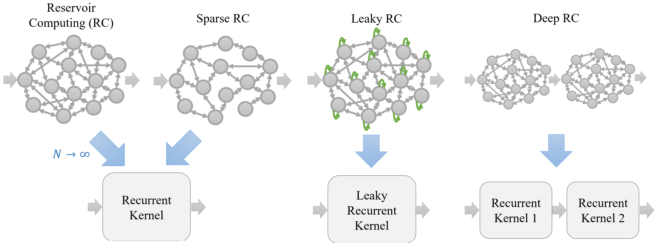
Figure 1: Recurrent Kernels associated with various Reservoir Computing topologies. RC and sparse RC converge to the same RK limit when the reservoir size $N\rightarrow\infty$. Leaky RC and Deep RC converge to their corresponding limits.

Deep Reservoir Computing stacks multiple reservoir layers to form a deep architecture also called a Deep Echo State Network (deepESN) [6]. The first layer operates like the reservoir in a shallow Reservoir Computing architecture and is fed by the external input, while each successive layer is fed by the output of the previous one. The reservoir layer of a deepESN can be expressed as:

$$\mathbf{x}_{l}^{(t+1)}=\frac{1}{\sqrt{N_{l}}}f\left(\sigma_{r}\mathbf{W}_{r}^{l}\mathbf{x}_{l}^{(t)}+\sigma_{i}\mathbf{W}_{i}^{l}\mathbf{u}_{l}^{(t)}\right)$$ (6)

where the index $l=1,\ldots,L$ describes the layer with a reservoir of size $N_{l}$, $\mathbf{u}_{l}^{(t)}$ is the input for the $l$-th layer:

$$\mathbf{u}_{l}^{(t)}=\begin{cases}\mathbf{i}^{(t)}\text{ if }l=1\\ \mathbf{x}_{l-1}^{(t+1)}\text{ if }l>1.\end{cases}$$ (7)

One of the main ideas is that each reservoir is encoding the recent past of its received input. Thus, the first layer has limited memory while the subsequent ones are able to extend this memory and build more complex representations of the input signal. It is possible to further add different leak rates to enforce slower dynamics for the deeper reservoir layers.

The output of a deepESN at each time step $t$ can be computed by applying any linear model to the different reservoir states. One commonly choose to define the linear model on the concatenation of all reservoir states; the output $\mathbf{o}^{(t)}$ is given by:

$$\mathbf{o}^{(t)}=\mathbf{W}_{\mathrm{out}}\left[\begin{matrix}\mathbf{x}_{1}^{(t)}\\ \mathbf{x}_{2}^{(t)}\\ \vdots\\ \mathbf{x}_{L}^{(t)}\end{matrix}\right]$$ (8)

where $\mathbf{W}_{\mathrm{out}}\in\mathbb{R}^{n\times\sum_{l}N_{l}}$ is a weight matrix that maps the concatenated reservoir states to the output. The concatenation of the reservoir states from each layer allows for the capture of information across multiple time scales, enabling the deepESN to model more complex temporal patterns.

The different variants presented above are not exclusive. For example, it is common to introduce different leak rates and sparse internal weight matrices to each layer of a deepESN.

Other strategies have also been proposed to alleviate the dense matrix multiplication by the reservoir weights. Structured Reservoir Computing [3] provides another alternative for reducing computational cost, where the reservoir weights are replaced by a structured transform instead. Next-generation Reservoir Computing [7] replaces the non-linear recurrent reservoir by an explicit mapping with polynomial combination of past inputs. As such, it can be interpreted as a non-recurrent temporal kernel.

2.3 Recurrent Kernels

In machine learning, kernels are functions that measure the similarity between pairs of data points, in a high-dimensional space to enable effective linear models. This mapping into the higher-dimensional feature space is often done implicitly by computing the scalar products between data points. This observation can be extended to Reservoir Computing. We consider two reservoirs $\mathbf{x}$ and $\mathbf{y}$ driven by the inputs $\mathbf{i}$ and $\mathbf{j}$ respectively, following the update equation (1). For conciseness, we assume $\sigma_{r}=\sigma_{i}=1$; equations for different values of reservoir and input scales can be obtained by substituting $\mathbf{x}^{(t)}$ by $\sigma_{r}\mathbf{x}^{(t)}$ and $\mathbf{i}^{(t)}$ by $\sigma_{i}\mathbf{i}^{(t)}$. The scalar product between two reservoir states can be expressed as:

$$\left(\mathbf{x}^{(t+1)}\right)^{\top}\mathbf{y}^{(t+1)} =\frac{1}{N}\sum_{l=1}^{N}f\left(\mathbf{w}_{r,l}^{\top}\mathbf{x}^{(t)}+\mathbf{w}_{i,l}^{\top}\mathbf{i}^{(t)}\right)\times$$

$$\qquad\qquad f\left(\mathbf{w}_{r,l}^{\top}\mathbf{y}^{(t)}+\mathbf{w}_{i,l}^{\top}\mathbf{j}^{(t)}\right)$$ (9)

where $\mathbf{w}_{r,l}$ and $\mathbf{w}_{i,l}$ denote the $l$-th line of $\mathbf{W}_{r}$ and $\mathbf{W}_{i}$ respectively. Thanks to the law of large numbers, this quantity converges when the reservoir size $N$ goes to infinity to a deterministic kernel function $k_{0}:\left(\mathbb{R}^{N+d}\right)^{2}\rightarrow\mathbb{R}$ defined as:

$$k_{0}\left(\mathbf{u}^{(t)},\mathbf{v}^{(t)}\right)=\int d\mathbf{w}p(\mathbf{w})f\left(\mathbf{w}^{\top}\mathbf{u}^{(t)}\right)f\left(\mathbf{w}^{\top}\mathbf{v}^{(t)}\right)$$ (10)

where we have introduced $\mathbf{u}^{(t)}=\left[\begin{matrix}\mathbf{x}^{(t)}\\ \mathbf{i}^{(t)}\end{matrix}\right]$, $\mathbf{v}^{(t)}=\left[\begin{matrix}\mathbf{y}^{(t)}\\ \mathbf{j}^{(t)}\end{matrix}\right]$, and $\mathbf{w}=\left[\begin{matrix}\mathbf{w}_{r}\\ \mathbf{w}_{i}\end{matrix}\right]$ a random vector of dimension $N+d$ with i.i.d. normal entries.

To properly define the associated Recurrent Kernel, we need to remove the dependence on the previous reservoir states $\mathbf{x}^{(t)}$ and $\mathbf{y}^{(t)}$, as they themselves depend on the random weights $\mathbf{W}_{r}$ and $\mathbf{W}_{i}$. This is possible if $k_{0}$ is an iterable kernel, i.e. if there exists $k:\mathbb{R}^{3}\rightarrow\mathbb{R}$ such that for all $\mathbf{u},\mathbf{v}\in\mathbb{R}^{N+d}$:

$$k_{0}(\mathbf{u},\mathbf{v})=k(\|\mathbf{u}\|^{2},\|\mathbf{v}\|^{2},\mathbf{u}^{\top}\mathbf{v}).$$ (11)

We show in Appendix that this is always the kernel associated to Reservoir Computing is always iterable, as soon as the weights are sampled from a gaussian distribution (or any rotationnally-invariant distribution $p(\mathbf{w})$). This is an extension of the statement in [3] that assumed translation or rotation-invariant kernels.

We define the recurrent kernel by replacing $\left(\mathbf{x}^{(t+1)}\right)^{\top}\mathbf{y}^{(t+1)}$ in Eq. (2.3) by $k^{(t+1)}\left(\mathbf{i}^{(t)},\mathbf{j}^{(t)},\ldots\right)$. Similarly, we replace in Eq. (11) $\left(\mathbf{u}^{(t)}\right)^{\top}\mathbf{v}^{(t)}$ by $k^{(t)}(\mathbf{i}^{(t-1)},\mathbf{j}^{(t-1)},\ldots)+\left(\mathbf{i}^{(t)}\right)^{\top}\mathbf{j}^{(t)}$, and perform the same operation for the norms (i.e. symmetric scalar products). This leads to the following definition of a Recurrent Kernel (RK) as a sequence of kernel functions $k^{(t)}:\left(\mathbb{R}^{d}\right)^{2t}\rightarrow\mathbb{R}$ for $t\in\mathbb{N}^{*}$:

$$\begin{cases}k^{(1)}\left(\mathbf{i}^{(0)},\mathbf{j}^{(0)}\right)&=k(1+\|\mathbf{i}^{(0)}\|^{2},1+\|\mathbf{j}^{(0)}\|^{2},\left(\mathbf{i}^{(t)}\right)^{\top}\mathbf{j}^{(t)})\\ k^{(t+1)}\left(\mathbf{i}^{(t)},\mathbf{j}^{(t)},\ldots\right)&=k(k^{(t)}(\mathbf{i}^{(t-1)},\mathbf{i}^{(t-1)},\ldots)+\|\mathbf{i}^{(t)}\|^{2},\\ &\qquad k^{(t)}(\mathbf{j}^{(t-1)},\mathbf{j}^{(t-1)},\ldots)+\|\mathbf{j}^{(t)}\|^{2},\\ &\qquad k^{(t)}(\mathbf{i}^{(t-1)},\mathbf{j}^{(t-1)},\ldots)+\left(\mathbf{i}^{(t)}\right)^{\top}\mathbf{j}^{(t)})\end{cases}$$ (12)

In the first line, we have initialized the RK by choosing $\|\mathbf{x}^{(0)}\|=\|\mathbf{y}^{(0)}\|=1$ and $\left(\mathbf{x}^{(0)}\right)^{\top}\mathbf{y}^{(0)}=0$. As Random Features are randomized approximations of kernel functions [15], Reservoir Computing can be interpreted as a randomized approximation of a well-defined Recurrent Kernel.

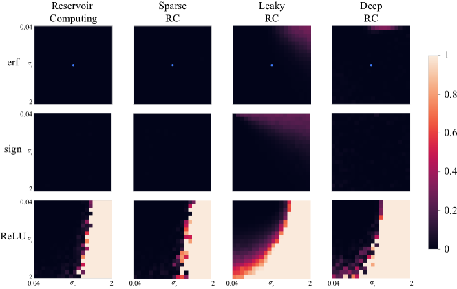
Figure 2: Convergence study of various Reservoir Computing topologies (columns) towards their corresponding Recurrent Kernel limits, for different activation functions $f$ (rows). For each case, the error metric $L$ (Eq. (18), smaller is better) is displayed for weight scaling factors $\sigma_{r}$, $\sigma_{i}$ between 0.04 and 2. Blue dot in the first row: typical operating point $\sigma_{r}=\sigma_{i}=1$.

One can then replace large-scale Reservoir Computing by Recurrent Kernels. To accomplish this, one must compute the recurrent kernels for each pair of training inputs, which are then placed into a matrix known as the Gram matrix. For instance, let us denote by $\mathbf{i}_{m}$, $m=1,\ldots,M$, the different inputs. The Gram matrix $\mathbf{G}^{(t)}\in\mathbb{R}^{M\times M}$ is defined for $t\in\mathbb{N}^{*}$ as:

$$\mathbf{G}^{(t)}=\left[k^{(t)}(\mathbf{i}_{n}^{(t-1)},\mathbf{i}_{m}^{(t-1)},\ldots)\right]_{n,m}$$ (13)

A linear model is trained using the Gram matrix and can be employed for making predictions.

Recurrent Kernels hold promise as a substitute for large-scale Reservoir Computing, as they offer comparable performance as the Reservoir Computing limit with infinitely-many neurons. However, the drawback is the computational time needed for prediction, as scalar products must be computed with each training input for use in the linear model. Additionally, due to their analytic formulation, Recurrent Kernels are well-suited for theoretical studies on Reservoir Computing [2].

Rigorously proving the convergence of Reservoir Computing to the Recurrent Kernel has proven challenging. Three assumptions are typically required [3]:

1. Lipschitz-continuity: the activation function is $l$-Lipschitz;

2. Contractivity: the scaling factor of the reservoir weights needs to satisfy $\sigma_{r}^{2}\leq 1/l$

3. Time-independence: the weight matrix is resampled at each time step.

Interestingly, convergence is usually observed in practice for a wider range of hyperparameters, despite these assumptions being violated.

3 Results

3.1 Extensions of Recurrent Kernels

The Recurrent Kernel for sparse Reservoir Computing corresponds to the same Recurrent Kernel as the non-sparse case. This implies that the performance of a sparse reservoir is equivalent to the one of a nonsparse one as soon as the number of neurons is large enough, typically a few hundreds. To obtain this result, the reservoir activations at each iteration needs not to be sparse, which is generally valid for Reservoir Computing. A more detailed study of the sparse case is provided in Appendix.

The Recurrent Kernel corresponding to Reservoir Computing with leak rate is defined by replacing the update equation of Eq. (12)

$$k^{(t+1)}(\mathbf{i}^{(t)},\mathbf{j}^{(t)},\ldots)= \ (1-a)^{2}k^{(t)}\left(\mathbf{i}^{(t-1)},\mathbf{j}^{(t-1)},\ldots\right)$$

$$+ a^{2}k(k^{(t)}(\mathbf{i}^{(t-1)},\mathbf{i}^{(t-1)},\ldots)+\|\mathbf{i}^{(t)}\|^{2},$$

$$\qquad k^{(t)}(\mathbf{j}^{(t-1)},\mathbf{j}^{(t-1)},\ldots)+\|\mathbf{j}^{(t)}\|^{2},$$

$$\qquad k^{(t)}(\mathbf{i}^{(t-1)},\mathbf{j}^{(t-1)},\ldots)+\left(\mathbf{i}^{(t)}\right)^{\top}\mathbf{j}^{(t)})$$ (14)

It requires several assumptions, most importantly that $f(u)$ is zero mean when $u$ is a normally-distributed random variable. The derivation is provided in Appendix. As described for the vanilla case of Recurrent Kernels, this limit is valid beyond these assumptions and we will study it numerically.

For Deep Reservoir Computing, we can write the kernel limit for each layer. We start by the first layer:

$$k^{(t+1)}_{1}\left(\mathbf{i}^{(t)},\mathbf{j}^{(t)},\ldots\right) =k(k^{(t)}_{1}(\mathbf{i}^{(t-1)},\mathbf{i}^{(t-1)},\ldots)+\|\mathbf{i}^{(t)}\|^{2},$$

$$\qquad k^{(t)}_{1}(\mathbf{j}^{(t-1)},\mathbf{j}^{(t-1)},\ldots)+\|\mathbf{j}^{(t)}\|^{2},$$

$$\qquad k^{(t)}_{1}(\mathbf{i}^{(t-1)},\mathbf{j}^{(t-1)},\ldots)+\left(\mathbf{i}^{(t)}\right)^{\top}\mathbf{j}^{(t)})$$ (15)

For the subsequent layers $l>1$, we obtain the recursive formula:

$$k^{(t+1)}_{l}\left(\mathbf{i}^{(t)},\mathbf{j}^{(t)},\ldots\right) =k(k^{(t)}_{l}(\mathbf{i}^{(t-1)},\mathbf{i}^{(t-1)},\ldots)+k^{(t+1)}_{l-1}(\mathbf{i}^{(t)},\mathbf{i}^{(t)},\ldots),$$

$$\qquad k^{(t)}_{l}(\mathbf{j}^{(t-1)},\mathbf{j}^{(t-1)},\ldots)+k^{(t+1)}_{l-1}(\mathbf{j}^{(t)},\mathbf{j}^{(t)},\ldots),$$

$$\qquad k^{(t)}_{l}(\mathbf{i}^{(t-1)},\mathbf{j}^{(t-1)},\ldots)+k^{(t+1)}_{l-1}(\mathbf{i}^{(t)},\mathbf{j}^{(t)},\ldots))$$ (16)

The Recurrent Kernel prediction is performed by concatenating the reservoir states of the different layers and using a linear model. This corresponds to a sum of the different Gram matrices:

$$k_{\mathrm{tot}}^{(t+1)}(\mathbf{i}^{(t)},\mathbf{j}^{(t)},\ldots)=\sum_{l}k_{l}^{(t+1)}(\mathbf{i}^{(t)},\mathbf{j}^{(t)},\ldots)$$ (17)

3.2 Convergence study

We show in Figure 2 a numerical convergence study of the various Reservoir Computing topologies to their respective Recurrent Kernel limits. Two random inputs of length 10 and dimension 100 are generated and fed to reservoirs of size 200. When applicable, the sparsity level is set at $s=0.8$ and the leak rate at $a=0.5$. For Deep Reservoir Computing, we use a sequence of two reservoirs of size 200.

We compute the final Gram matrix $G^{\mathrm{RC}}$ at time $T+1=11$. This Gram matrix is compared with the Gram matrix $G^{\mathrm{RK}}$ obtained using the associated Recurrent Kernel. The metric displayed is the Frobenius norm between the final Gram matrices:

$$L=\left\|G_{\mathrm{RC}}^{(T+1)}-G_{\mathrm{RK}}^{(T+1)}\right\|^{2}_{F}.$$ (18)

This metric is computed for different values of the reservoir weight standard deviations $\sigma_{r}$ and $\sigma_{i}$ which dictate the dynamics of the reservoir between 0 and 2. We perform this study for three typical activation functions: erf (differentiable and bounded), ReLU (sub-differentiable and unbounded), and sign (discontinuous and bounded).

We see that in the sparse case, the convergence is fundamentally similar to non-sparse Reservoir Computing. We observe convergence over the whole parameter range for bounded activation functions. For ReLU, convergence is achieved for small values of $\sigma_{r}$ with a slight dependence on $\sigma_{i}$. This is due to errors accumulating with the ReLU activation function.

For leaky Reservoir Computing and Deep Reservoir Computing, the convergence region is generally smaller. For bounded activations, it typically does not converge for large $\sigma_{r}$ and small $\sigma_{i}$. This typically corresponds to an unstable case [2] that is not used in practice. For ReLU, convergence is achieved for a range of parameters $(\sigma_{r},\sigma_{i})$ slightly smaller than the non-leaky case. When the reservoir or input weights are large, error accumulates and activations diverge, more evidence is provided in Appendix.

3.3 How to choose sparsity level

Our framework enables us to compare reservoirs with different sparsity levels. Since Sparse RC converges to the same limit regardless of the level of sparsity, we compute the normalized error metric as defined in Eq. (18) for different reservoir sizes in Fig. 3 (top row). The error metric being dependent on the reservoir size, we normalize it between 0 and 1 to represent all curves on the same graph. The error metric being dependent on the stochastic realization of the weights, we perform a Monte-Carlo estimation with at least $10^{4}$ realizations to decrease the estimation variance.

We observe that sparse RC achieves the same convergence as RC which corresponds to $s=1$. One can decrease the sparsity level until a threshold below which the approximation error increases. This threshold decreases with the reservoir size: larger reservoirs handle low sparsity levels better.

In the bottom row of Fig. 3, we plot the threshold defined as $10\%$ of the non-sparse limit. We see that we can decrease the sparsity factor quite dramatically: for a reservoir size $N=1000$, we can decrease the sparsity rate down to $s=0.02$. This value is below the typical sparsity level of 0.05 [17, 5], which could lead to further computational and memory savings. Note that the decrease does not seem to be inversely-proportional to the reservoir size. We suspect that as the reservoir size increases, it becomes a better approximation of the RK limit and it becomes difficult to reduce $s$ while keeping the same approximation quality.

3.4 Optimal Deep Reservoir Computing sizes

In practice, our study enables to study how to set the subsequent reservoir weights. Should we choose the first or second reservoir to be larger? To investigate this question, we compute the previous metric given in Eq. (18) for a fixed computational budget $n_{1}^{2}+n_{2}^{2}=2\times 200^{2}$. This quadratic scaling corresponds to the computational and memory complexity of the dense matrix multiplication, which is the limiting factor in Eq. (1). Each point is an average of 4000 repetitions.

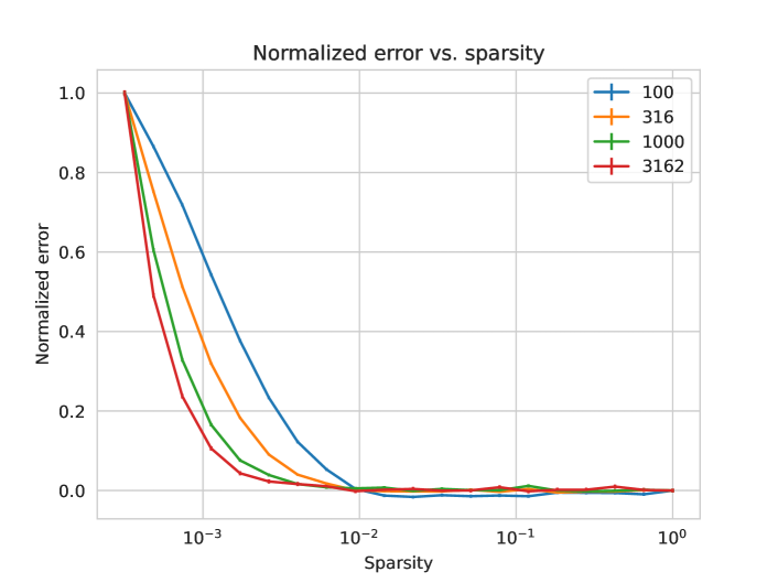
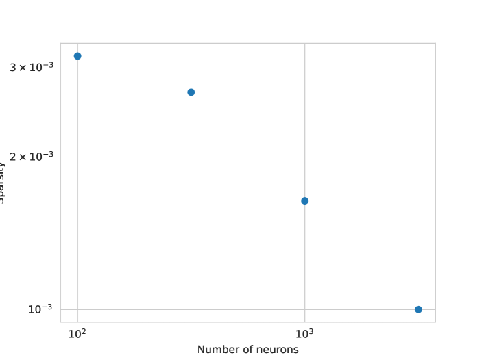
Figure 3: (Top) Error metric (Eq. (18)) normalized between 0 and 1 as a function of sparsity for different reservoir sizes. (Bottom) Sparsity threshold above which the error metric is within $10\%$ of the non-sparse limit. This gives an admissible sparsity level which decreases with the reservoir size.

The metric as a function of $n_{1}$ is depicted in Fig. 4. We see that the extreme cases yield high error. When the first reservoir size is too small, the error of the first RK is detrimental even though the second reservoir is closer to its limit. Similarly, the second reservoir size cannot be too small or the second recurrent kernel is not well approximated. There is a wide region for which the error is relatively small.

We performed a Nelder-Mead optimization to find the optimal reservoir sizes for different depths. For $L=2$, we obtain $n_{1},n_{2}=209,190$, for $L=2$, we obtain $n_{1},n_{2},n_{3}=207,202,190$. Thus, the optimal shapes have first reservoir sizes that are larger than subsequent ones. This decreases the noise that is transmitted to the next layers.

In a nutshell, a good rule of thumb to choose the reservoir sizes in Deep Reservoir Computing is to choose them all equal. First reservoirs can be chosen slightly (5%) larger than the last ones to decrease further the distance with the asymptotic limit performance.

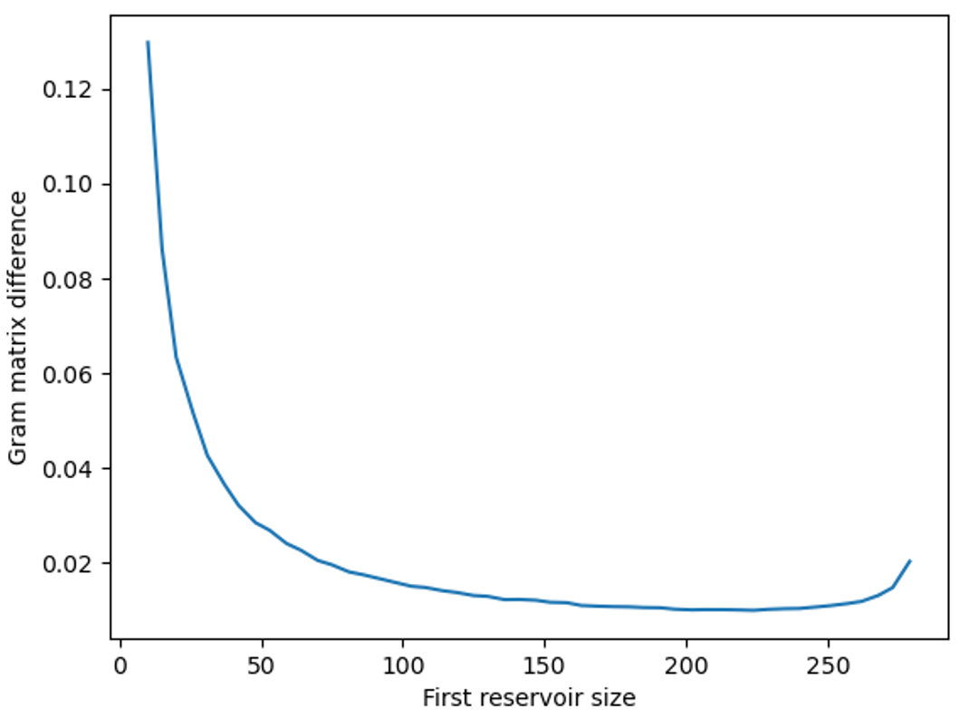
Figure 4: Error metric (Eq. (18)) for Deep Reservoir Computing for varying reservoir sizes. We vary the first layer size $N_{1}$ for a fixed computational budget $N_{1}^{2}+N_{2}^{2}=2\times 200^{2}$.

4 Discussion

In our study, we have derived the Recurrent Kernel limit of different reservoir topologies. We have shown that different topologies can lead to the same asymptotic limit. More specifically, the presence of sparsity does not affect convergence at all, which justifies the sparse initialization of reservoir weights to speed up computation. Convergence has been studied numerically and validated for a wide range of parameters, especially for bounded activation functions. Finally, we have derived how Recurrent Kernels extend to Deep Reservoir Computing, and how it sheds new insight on how to set the consecutive reservoir sizes.

It may be interesting in the future to optimize for computational cost in practice, through the use of a dedicated sparse linear algebra library and compare with structured transforms. Other topologies based on random connections may also be explored, such as: random features [15] and extreme learning machines [8], which approximate a kernel in expectation with non-recursive random embeddings; gaussian processes [13], stochastic processes defined by a mean and a covariance, which can give an accurate estimate of the uncertainty in regression tasks ; and random vector functional link networks [14], wherein the weights of the network are generated randomly and output weights are computed analytically.

Appendix A Iterable kernels for any rotationally-invariant distribution

We prove here that the kernel limit defined in Eq. (10) is iterable as soon as the weights are random gaussian, for any activation function $f$.

For any fixed timestep $t$, using the invariance by rotation of $p(\mathbf{w})$, we can change the basis to:

$$\begin{cases}\mathbf{u}^{(t)}=u_{1}\mathbf{e}_{1}\\ \mathbf{v}^{(t)}=v_{1}\mathbf{e}_{1}+v_{2}\mathbf{e}_{2}\end{cases}$$ (19)

with $\mathbf{e}_{1}$ and $\mathbf{e}_{2}$ the first two vectors of an orthonormal basis. Importantly, $u_{1}$, $v_{1}$, and $v_{2}$ only depend on scalar products $\|\mathbf{u}^{(t)}\|^{2}$, $\|\mathbf{v}^{(t)}\|^{2}$, and $\left(\mathbf{u}^{(t)}\right)^{\top}\mathbf{v}^{(t)}$:

$$\begin{cases}u_{1}=\|\mathbf{u}^{(t)}\|\\ v_{1}=\left(\mathbf{v}^{(t)}\right)^{\top}\mathbf{e}_{1}=\frac{1}{\|\mathbf{u}^{(t)}\|}\left(\mathbf{v}^{(t)}\right)^{\top}\mathbf{u}^{(t)}\\ v_{2}=\sqrt{\|\mathbf{v}^{(t)}\|^{2}-v_{1}^{2}}=\sqrt{\|\mathbf{v}^{(t)}\|^{2}-\frac{1}{\|\mathbf{u}^{(t)}\|^{2}}\left(\left(\mathbf{v}^{(t)}\right)^{\top}\mathbf{u}^{(t)}\right)^{2}}\end{cases}$$ (20)

The kernel limit in Eq. (10) can be rewritten as an integral over two gaussian random variables $w_{1}$ and $w_{2}$:

$$k_{0}\left(\mathbf{u}^{(t)},\mathbf{v}^{(t)}\right) =\int dw_{1}dw_{2}p(w_{1})p(w_{2})f(w_{1}u_{1})f(w_{1}v_{1}+w_{2}v_{2})$$ (21)

$$\equiv k\left(\|\mathbf{u}^{(t)}\|^{2},\|\mathbf{v}^{(t)}\|^{2},\left(\mathbf{u}^{(t)}\right)^{\top}\mathbf{v}^{(t)}\right).$$ (22)

Thus, the kernel limit for all RC algorithms with random gaussian weights is an iterable kernel, allowing us to define an associated Recurrent Kernel. As we see in this proof, it can be extended to any rotationally-invariant distribution of weights $p(\mathbf{w})$.

Appendix B Sparse Random Features

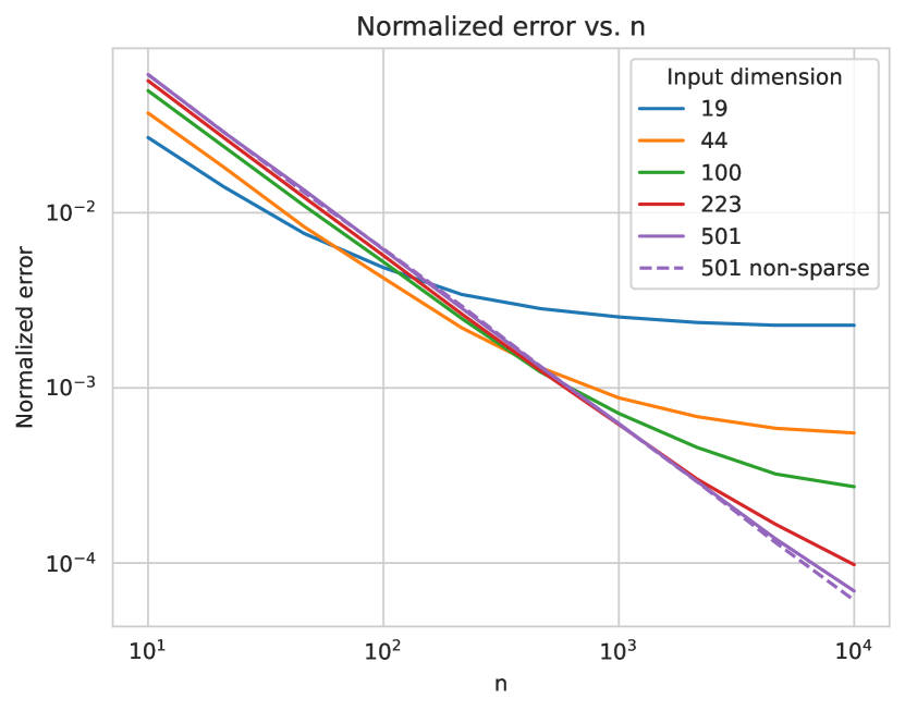
Figure 5: Approximation error Eq. (24) of sparse Random Features as a function of Random Feature dimension $n$. An example of non-sparse convergence is given with dashed lines.

We investigate the convergence of Eq. (2.3) to its single-step limit defined in Eq. (10) when the weights $\mathbf{w}$ are sparse. This can be interpreted as a sparse Random Feature embedding.

We initialize a random vector $\mathbf{u}\in\mathbb{R}^{d}$ (i.i.d. uniform between 0 and 1) and generate Random Features embedding following:

$$\psi(\mathbf{u})=f(\mathbf{W}\mathbf{u}).$$ (23)

$\mathbf{W}\in\mathbb{R}^{n\times d}$ is an i.i.d. random matrix and $f$ an element-wise non-linearity. In this context, we can also define the single-step kernel function $k_{0}(\mathbf{u},\mathbf{v})$ of Eq. (10). The approximation error is given by:

$$l=|\left(\psi(\mathbf{u})\right)^{\top}\psi(\mathbf{v})-k_{0}(\mathbf{u},\mathbf{v})|^{2}.$$ (24)

This quantity is displayed in Fig. 5 as a function of Random Feature dimension $n$, for different input dimension and for non-sparse (gaussian) and sparse ($s=0.1$) random vector $\mathbf{w}$. It is averaged over $10^{4}$ repetitions.

First, we see that in the non-sparse case, convergence is achieved with a fixed rate; only a single curve is displayed as the non-sparse curves only differ by a prefactor. In the sparse case, convergence is similar for small $n$, until a certain value after which the approximation error reaches a plateau.

In Reservoir Computing, input and output sizes $d$ and $n$ are similar, we see that this operating point is before this threshold for $s=0.1$. Instead, the sparsity level $s$ can be varied as displayed in Fig. 3.

Appendix C Derivation of the limit for leaky Reservoir Computing

We motivate here the definition of the leaky Recurrent Kernel as defined in Eq. (3.1). Using the leaky RC update equation (5), we have:

$$\left(\mathbf{x}^{(t+1)}\right)^{\top}\mathbf{y}^{(t+1)} =\left(\frac{a}{\sqrt{N}}f\left(\mathbf{W}\mathbf{u}^{(t)}\right)+(1-a)\mathbf{x}^{(t)}\right)^{\top}$$ (25)

$$\qquad\qquad\left(\frac{a}{\sqrt{N}}f\left(\mathbf{W}\mathbf{v}^{(t)}\right)+(1-a)\mathbf{y}^{(t)}\right)$$

$$=\frac{a^{2}}{N}f\left(\mathbf{W}\mathbf{u}^{(t)}\right)^{\top}f\left(\mathbf{W}\mathbf{v}^{(t)}\right)$$ (26)

$$\qquad\qquad+\frac{a(1-a)}{\sqrt{N}}f\left(\mathbf{W}\mathbf{u}^{(t)}\right)^{\top}\mathbf{y}^{(t)}$$

$$\qquad\qquad+\frac{a(1-a)}{\sqrt{N}}f\left(\mathbf{W}\mathbf{v}^{(t)}\right)^{\top}\mathbf{x}^{(t)}$$

$$\qquad\qquad+(1-a)^{2}\left(\mathbf{x}^{(t)}\right)^{\top}\mathbf{y}^{(t)}$$

The first term converges to the non-sparse limit $k_{0}\left(\mathbf{u}^{(t)},\mathbf{v}^{(t)}\right)$. The last term corresponds to the previous recurrent kernel limit $k^{(t)}(\mathbf{i}^{(t-1)},\mathbf{j}^{(t-1)},\ldots)$. Furthermore, we neglect the two cross-product terms, which results in Eq. (3.1). These cross-products are not straightforward to analyze as the previous reservoir state $\mathbf{y}^{(t)}$ also depend on the random weights $\mathbf{W}$.

References

- Damicelli et al. [2022] Damicelli, F., Hilgetag, C.C., Goulas, A., 2022. Brain connectivity meets reservoir computing. PLoS Computational Biology 18, e1010639.
- Dong et al. [2022] Dong, J., Börve, E., Rafayelyan, M., Unser, M., 2022. Asymptotic stability in reservoir computing, in: 2022 International Joint Conference on Neural Networks (IJCNN), IEEE. pp. 01–08.
- Dong et al. [2020] Dong, J., Ohana, R., Rafayelyan, M., Krzakala, F., 2020. Reservoir computing meets recurrent kernels and structured transforms. Advances in Neural Information Processing Systems 33, 16785–16796.
- Gallicchio [2020] Gallicchio, C., 2020. Sparsity in reservoir computing neural networks, in: 2020 International Conference on Innovations in Intelligent SysTems and Applications (INISTA), IEEE. pp. 1–7.
- Gallicchio and Micheli [2011] Gallicchio, C., Micheli, A., 2011. Architectural and markovian factors of echo state networks. Neural Networks 24, 440–456.
- Gallicchio et al. [2017] Gallicchio, C., Micheli, A., Pedrelli, L., 2017. Deep reservoir computing: A critical experimental analysis. Neurocomputing 268, 87–99.
- Gauthier et al. [2021] Gauthier, D.J., Bollt, E., Griffith, A., Barbosa, W.A., 2021. Next generation reservoir computing. Nature communications 12, 5564.
- Huang et al. [2006] Huang, G.B., Zhu, Q.Y., Siew, C.K., 2006. Extreme learning machine: theory and applications. Neurocomputing 70, 489–501.
- Jaeger [2001] Jaeger, H., 2001. The “echo state” approach to analysing and training recurrent neural networks-with an erratum note. Bonn, Germany: German National Research Center for Information Technology GMD Technical Report 148, 13.
- Jaeger and Haas [2004] Jaeger, H., Haas, H., 2004. Harnessing nonlinearity: Predicting chaotic systems and saving energy in wireless communication. science 304, 78–80.
- Jaeger et al. [2007] Jaeger, H., Lukoševičius, M., Popovici, D., Siewert, U., 2007. Optimization and applications of echo state networks with leaky-integrator neurons. Neural networks 20, 335–352.
- Lukoševičius and Jaeger [2009] Lukoševičius, M., Jaeger, H., 2009. Reservoir computing approaches to recurrent neural network training. Computer Science Review 3, 127–149.
- MacKay et al. [1998] MacKay, D.J., et al., 1998. Introduction to gaussian processes. NATO ASI series F computer and systems sciences 168, 133–166.
- Malik et al. [2023] Malik, A.K., Gao, R., Ganaie, M., Tanveer, M., Suganthan, P.N., 2023. Random vector functional link network: recent developments, applications, and future directions. Applied Soft Computing , 110377.
- Rahimi and Recht [2007] Rahimi, A., Recht, B., 2007. Random features for large-scale kernel machines. Advances in neural information processing systems 20.
- Tanaka et al. [2019] Tanaka, G., Yamane, T., Héroux, J.B., Nakane, R., Kanazawa, N., Takeda, S., Numata, H., Nakano, D., Hirose, A., 2019. Recent advances in physical reservoir computing: A review. Neural Networks 115, 100–123.
- Xue et al. [2007] Xue, Y., Yang, L., Haykin, S., 2007. Decoupled echo state networks with lateral inhibition. Neural Networks 20, 365–376.