Precision Mars Entry Navigation with Atmospheric Density Adaptation via Neural Networks

Abstract

Discrepancies between the true Martian atmospheric density and the onboard density model can significantly impair the performance of spacecraft entry navigation filters. This work introduces a new approach to online filtering for Martian entry by using a neural network to estimate atmospheric density and employing a consider analysis to account for the uncertainty in the estimate. The network is trained on an exponential atmospheric density model, and its parameters are dynamically adapted in real time to account for any mismatches between the true and estimated densities. The adaptation of the network is formulated as a maximum likelihood problem, leveraging the measurement innovations of the filter to identify optimal network parameters. The incorporation of a neural network enables the use of stochastic optimizers known for their efficiency in the machine learning domain within the context of the maximum likelihood approach. Performance comparisons against previous approaches are conducted in various realistic Mars entry navigation scenarios, resulting in superior estimation accuracy and precise alignment of the estimated density with a broad selection of realistic Martian atmospheres sampled from perturbed Mars-GRAM data.

1 Introduction

Among the most demanding challenges encountered in spacecraft navigation is atmospheric entry, particularly Martian entry. The entry phase is characterized by its intense dynamics, scarcity of available measurements, and uncertain atmospheric information [1]. While knowledge of the Martian atmosphere, weather, and seasons has improved over the last decades, it is not as accurately predicted as the atmosphere of Earth. Large uncertainties in models used to estimate the Martian atmosphere can make navigation during the entry phase challenging and can significantly degrade guidance solutions affecting landing accuracy [2]. The development of standard Entry, Descent, and Landing (EDL) systems is additionally complicated by atmospheric variability across Martian years. These systems typically employ a correction mechanism, adjusting a nominal exponential profile with a multiplicative factor based on the drag force experienced by the spacecraft [3]. However, constraining density estimation to an exponential profile poses challenges due to the significant atmospheric dust content on Mars, known to increase the temperature of the lower atmosphere and subsequently reduce its density [4]. As a result of this, future human and robotic Mars exploration missions require an improvement in navigation solutions by several orders of magnitude over the current state-of-the-art [5].

Traditionally, Mars entry missions have used inertial measurement units (IMU) for navigation, in lieu of onboard models of non-conservative forces. However, the drawback of IMU-based solutions lies in their tendency to drift over time, especially in the absence of external measurements. When employed for state correction rather than propagation, IMU measurements alone can result in rendering most estimation states unobservable [6]. Due to this, different techniques have been explored to improve the navigation solutions during Martian entry. In early efforts of using only IMU measurements for entry navigation, Zanetti and Bishop [7] successfully quantified the accuracy of state estimates through dead-reckoning during a standard Mars atmospheric entry. Following this approach, Lou et al. [8] presented a strategy attempting to mitigate the effects of unobservable uncertain parameters through consider analysis during entry, achieving promising results. Additionally, Jiang et al. [9] introduced a more accurate multi-sensor strategy, where instead of only using an IMU for navigation, information from real-time flush air data system, a single orbiting radio beacon, and an IMU were fused using an unscented Kalman filter, providing better estimation results. More recently, the integration of aerodynamic pressure and aerothermal sensor data for real-time navigation has been proposed [10]. Nevertheless, most of these solutions encounter a common challenge: the use of an onboard exponential atmospheric density model, or reliance on external measurements like orbiting or surface beacons. These assumptions may pose difficulties when faced with real density profiles, potentially leading to filter divergence. Furthermore, it is worth noting that due to the presence of the heat-shield cover, onboard optical or radio navigation may not be available during entry [10]. Currently, a promising research area for entry navigation involves addressing the atmospheric uncertainty, offering potential improvements in estimation accuracy for Mars entry missions.

The descent and landing phases are typically supported by sensors such as altimeters, velocimeters, or LIDARs, which can aid the navigation solution [11, 12]. Since these sensors are not available during the entry phase, this segment presents the most significant challenge for navigation performance. Due to the limited availability of sensors during entry, accurate density estimation becomes crucial. Correctly estimating atmospheric density and quantifying its inherent uncertainty can greatly improve navigation outputs, thus enhancing overall precision landing performance. A range of methodologies have been investigated to address the atmospheric uncertainties within the Martian environment, with the aim of improving the performance of EDL systems. These approaches can be categorized into two main groups: offline reconstructions, which involves working with real data acquired during the entry phase, and online estimation techniques designed for use during the entry phase. Dutta et al. [13] conducted an analysis of various estimation techniques, including the extended Kalman filter (EKF) and the unscented Kalman filter (UKF) for offline reconstruction. In their work, the main objective was to reconstruct the vehicle’s trajectory, aerodynamic coefficients, and the atmospheric profile experienced by the system in an offline context. Subsequently, in their follow-up work [14], they demonstrated how adaptive filtering techniques, such as covariance matching [15], could enhance the estimation performance of aerodynamic coefficients and atmospheric properties. These advanced techniques were later employed to successfully reconstruct atmospheric properties using real data acquired by the Mars Science Laboratory (MSL) [16].

To improve the precision of filtering techniques in online estimation for EDL, various strategies have also been explored. A common solution involves carrying a nominal density onboard the filter and augmenting the system state to estimate a correction factor that accounts for the deviation between the nominal density and the actual density experienced by the system [10, 2]. In addition, machine learning approaches have also been used for density estimation in EDL problems. Wagner et al. [17] used an ensemble of neural networks to dynamically adapt to real-time changes in atmospheric properties during Martian entry. Additionally, Amato and McMahon [18] employed a long short-term memory network to estimate atmospheric density based on inertial measurements and guidance commands. Most recently, Roelke et al. [19] introduced two density profile prediction techniques for aerocapture, using density histories computed from navigation measurements to enhance targeting accuracy.

In this work, we propose a new approach to onboard filtering for Martian entry by using a neural network (trained pre-flight on a simplified model retrieved from Mars-GRAM trajectories) to estimate atmospheric density and accounting for atmospheric uncertainty through a consider approach. The atmospheric mismatch between the true density and the model used by the filter is addressed by adapting the parameters of the network in real-time using the measurement innovations of the navigation filter. The adaptation of the network is performed using aerodynamic pressure measurements, aerothermal sensor data, and an IMU, mirroring sensor configurations from prior Martian EDL missions [20, 21, 22]. By leveraging the capabilities of state-of-the-art stochastic optimizers, nonlinear activation functions, and automatic differentiation, the adaptation step is posed as a maximum likelihood (ML) problem, resulting in consistent filtering performance and accurate estimation of the true density.

The remainder of this paper is organized as follows: First, a background of Martian entry is provided in Section 2. Previous approaches to density adaptation are introduced in Section 3, and the approach to density adaptation using neural networks is presented in Section 4. The performance of the new approach is compared to previous approaches on a realistic Mars entry navigation scenario in Section 5. Finally, Section 6 provides conclusions and outlines future work opportunities.

2 Martian Entry

This section provides insight into the dynamics, measurement, and atmospheric density models used in Martian entry. The aim of this analysis is to emphasize the importance of acquiring an accurate atmospheric density estimate during the entry phase. A clear understanding of these fundamentals is important for recognizing the crucial role that accurate density estimation plays in mission success [1].

2.1 Dynamics

The dynamics of entry vehicles during Martian entry are often represented using a simplified three degrees-of-freedom (3-DOF) model. In this approach and for the entirety of this work, point mass dynamics are assumed, meaning that no consideration is given to attitude dynamics - a common convention observed in prior literature [23, 6, 24]. The position of the vehicle is described in terms of planet-centric coordinates, which include the planet-centric radius ($r$), latitude ($\phi$), and longitude ($\theta$) [24],

$$\dot{r} =v\sin(\gamma),$$ (1)

$$\dot{\phi} =\frac{\cos(\gamma)\sin(\psi)}{r}{v},$$ (2)

$$\dot{\theta} =\frac{\cos(\gamma)\cos(\psi)}{r\cos(\phi)}v.$$ (3)

The use of planet-centric latitude and longitude ($\phi$ and $\theta$) facilitates the application of spherical equations of motion, even when dealing with a non-spherical planet, as the radius of the planet is allowed to vary with latitude and longitude [24]. The velocity ($v$), flight path angle ($\gamma$), and heading angle ($\psi$) are defined relative to the planet surface and are based on the vehicle-carried local horizontal frame (LH). The flight path angle is defined as negative-down and the heading angle is defined in the horizontal plane where $0^{\circ}$ is due East and due North is $90^{\circ}$ [24]. The equations describing the time evolution of the velocity-related terms are given by:

$$\dot{v} =-D-g\sin(\gamma)+\omega^{2}r\cos(\phi)\left[\sin(\gamma)\cos(\phi)-\cos(\gamma)\sin(\phi)\sin(\psi)\right],$$ (4)

$$\dot{\gamma} =\frac{1}{v}\left[L\cos(\sigma)-g\cos(\gamma)+\frac{v^{2}}{r}\cos(\gamma)+2\omega v\cos(\phi)\cos(\psi)\right]$$ (5)

$$+\frac{1}{v}\left[\omega^{2}r\cos(\phi)\left(\cos(\gamma)\cos(\phi)+\sin(\gamma)\sin(\phi)\sin(\psi)\right)\right],$$

$$\dot{\psi} =\frac{1}{v}\left[L\frac{\sin(\sigma)}{\cos(\gamma)}-\frac{v^{2}}{r}\cos(\gamma)\cos(\psi)\tan(\phi)+2\omega v\left(\tan(\gamma)\cos(\phi)\sin(\psi)-\sin(\phi)\right)\right]$$ (6)

$$-\frac{1}{v}\left[\frac{\omega^{2}r}{\cos(\gamma)}\sin(\phi)\cos(\phi)\cos(\psi)\right],$$

where $\omega$ represents the planetary rotation rate, $g$ is the planetary gravity, $\sigma$ is the bank angle, and the lift ($L$) and drag ($D$) accelerations are defined as follows:

$$D =\frac{1}{2}\rho\left(\cdot\right)v_{\infty}^{2}\frac{C_{d}S}{m},$$ (7)

$$L =\frac{1}{2}\rho\left(\cdot\right)v_{\infty}^{2}\frac{C_{l}S}{m}.$$ (8)

with $v_{\infty}=v-W$, where $W$ represents the wind velocity. The parameter $\rho\left(\cdot\right)$ is the atmospheric density, where the notation $(\cdot)$ signifies its dynamic nature during the entry phase. Given the dependency of lift and drag accelerations on atmospheric density, all velocity-related terms become directly influenced by changes in atmospheric density. As a result, the temporal evolution of the position implicitly relies on atmospheric density variations.

Given the substantial hypersonic speeds associated with the entry phase, wind velocities are considerably lower compared to the velocity of the vehicle, i.e., $v/W\ll 1$ [18]. In such cases, it is reasonable to make the approximation that $v_{\infty}\approx v$. Moreover, for brief-duration flights such as the entry phase in EDL, the impact of planetary rotation can be deemed negligible [10]. Hence, by omitting terms related to planetary rotation and assuming a first-order gravity model, the equations governing velocity parameters simplify to:

$$\dot{v} =-\frac{1}{2}\rho\left(\cdot\right)v^{2}\frac{C_{d}S}{m}-\frac{\mu}{r^{2}}\sin(\gamma),$$ (9)

$$\dot{\gamma} =\frac{1}{v}\left[\frac{1}{2}\rho\left(\cdot\right)v^{2}\frac{C_{l}S}{m}\cos(\sigma)-\frac{\mu}{r^{2}}\cos(\gamma)+\frac{v^{2}}{r}\cos(\gamma)\right],$$ (10)

$$\dot{\psi}=\frac{1}{v}\left[\frac{1}{2}\rho\left(\cdot\right)v^{2}\frac{C_{l}S}{m}\frac{\sin(\sigma)}{\cos(\gamma)}-\frac{v^{2}}{r}\cos(\gamma)\cos(\psi)\tan(\phi)\right].$$ (11)

By reviewing the dynamics that govern Martian entry, it becomes evident that errors in the estimation of atmospheric density can significantly impact the dynamics, leading to a considerable degradation in the propagation of filtering states. This emphasizes just how crucial it is to attain an accurate estimate of density for navigation solutions.

2.2 Onboard Sensors

The measurement model of the onboard sensors typically used in EDL missions is closely tied to the atmospheric density estimate as well. In this work, three distinct onboard sensors are under consideration. These sensors encompass an IMU, a cluster of pressure sensors strategically placed on the heat shield of the vehicle, and a suite of thermocouples situated on the forebody of the vehicle. These sensors are carefully selected to replicate the sensor configurations used in past Martian EDL missions [10, 20, 21, 22]. The IMU measures the non-gravitational accelerations encountered by the entry vehicle. In this work, these measurements are conducted relative to the body frame, as follows:

$$\tilde{\bm{a}}^{b}=T_{v}^{b}\bm{a}^{v}+\bm{\eta}_{\bm{a}},$$ (12)

where $\bm{\eta}_{\bm{a}}\in\mathbb{R}^{3}$ represents measurement noise, $T_{v}^{b}$ is the transformation matrix to change coordinates from velocity frame to body frame, and $\bm{a}^{v}\in\mathbb{R}^{3}$ are the non-gravitational accelerations in the velocity frame defined as:

$$\bm{a}^{v}=\begin{bmatrix}-D&L\sin\left(\sigma\right)&L\cos\left(\sigma\right)\end{bmatrix}^{\mathrm{T}}.$$ (13)

The pressure sensors are assumed to offer a reasonably accurate evaluation of the stagnation-point pressure, while the thermocouples are assumed to provide real-time measurements of the heating rate. It is important to acknowledge that the precision of these measurements may vary according to the flight regime. For instance, pressure transducers optimized for hypersonic flight may not deliver satisfactory results during supersonic flight. Nevertheless, this work assumes the availability of measurements throughout the entire entry stage. The dynamic pressure measurement, assuming an aggregate measurement from all relevant sensor arrays, is expressed as follows [10]:

$$\tilde{q}=\frac{1}{2}\rho\left(\cdot\right)v^{2}+\eta_{q}.$$ (14)

The measured convective heating rate is modeled by the Sutton-Graves relation, such that [25, 26]:

$$\tilde{\dot{Q}}_{s}=k\left(\frac{\rho\left(\cdot\right)}{R_{n}}\right)^{\frac{1}{2}}v^{3}+\eta_{\dot{Q}_{s}},$$ (15)

where $k=1.9027\times 10^{-4}$ kg^1/2m^-1, $R_{n}$ is the vehicle nose radius and $w_{\dot{Q}_{s}}\in\mathbb{R}$ is measurement noise. These equations further emphasize the critical importance of having an accurate atmospheric density estimate, as they all rely on this fundamental parameter. This connection illustrates how easily a navigation system can diverge when confronted with inaccurate estimates or inaccurate density models stored in the onboard computer of the vehicle, emphasizing the critical role of obtaining a highly accurate density estimate for mission success and safety.

2.3 Density Models

To model Martian atmospheric density, various approaches are available, ranging from more intricate models for increased accuracy to simpler equations for faster estimates, although with reduced precision. The most straightforward equation for modeling atmospheric density is based on an exponential law, assuming isothermal equilibrium [27]. This model is represented by the equation:

$$\hat{\rho}=\rho_{0}\exp\left(-\frac{(r-r_{0})}{h_{s}}\right),$$ (16)

where $r_{0}$ represents the reference radial position, $\rho_{0}$ is the density at the reference radial position, and $h_{s}$ stands for the atmospheric scale height. It is worth noting that while the atmosphere is not isothermal at all altitudes, the parameters in (16) can be adjusted piece-wise to better align with the real atmospheric density. However, as previously mentioned, constraining Martian density to an exponential profile can be challenging due to the variability in dust content, seasonal changes, and wind patterns [4]. In response to potential errors in the exponential model, the COSPAR model was developed using data collected from Viking 1, Viking 2, and Mariner missions [1]. Although lacking consideration for factors like longitude, latitude, seasonal variations, and dust content, the COSPAR model offers more precision than the basic exponential model. The simplified COSPAR model is expressed as a modified exponential equation,

$$\hat{\rho}=\rho_{0}\exp\left\{-\beta_{\rho}\left(r-r_{0}\right)+\gamma_{\rho}\cos\left[\omega_{\rho}\left(r-r_{0}\right)\right]+\delta_{\rho}\sin\left[\omega_{\rho}\left(r-r_{0}\right)\right]\right\},$$ (17)

where $\beta_{\rho},\gamma_{\rho},\omega_{\rho}$ and $\delta_{\rho}$ are nominal coefficients adjustable to better fit real atmospheric data. Both the exponential and COSPAR models rely on ad hoc parametrizations for estimating atmospheric density.

The Mars Global Reference Atmospheric Model (GRAM) 2010 represents a significant improvement in atmospheric modeling compared to previous models. Mars-GRAM is an engineering-level atmospheric model constructed using input data tables derived from NASA Ames Mars General Circulation Model (MGCM) and the University of Michigan Mars Thermospheric General Circulation Model (MTGCM) outputs. This model has undergone validation against Radio Science and thermal emission spectrometer (TES) data, encompassing both nadir and limb observations. Additionally, it can model potential perturbations in the atmosphere, a feature frequently employed in Monte Carlo simulations for high-fidelity engineering [28].

While Mars-GRAM excels in providing realistic estimates for potential atmospheric density profiles encountered during entry missions, it is usually avoided for online estimation due to its substantial computational overhead. Instead, online estimation approaches commonly use simplified models paired with adaptive techniques, validated through Monte Carlo simulations using truth trajectories propagated using atmospheric density values obtained from Mars-GRAM [2].

3 Approaches to Density Adaptation

As models cannot provide a perfect estimation of the atmospheric density, various adaptive techniques can be used to address potential errors or unforeseen behavior that the vehicle may encounter during the entry phase. The first approach involves covariance matching, wherein adjustments are made to the process noise and measurement covariance matrices to align with the state and measurement innovations in the navigation filter. The second technique entails the estimation of correction parameters, used to rectify a nominal density profile established during the offline phases of the navigation filter design. Lastly, multiple model adaptive estimation can also be used for this purpose, where a bank of estimators operates in parallel, yielding a more robust estimate by considering different density profiles. This section delves into the presentation and discussion of each of these approaches.

Covariance matching techniques have found utility in atmospheric reconstruction due to the inherent uncertainty in atmospheric parameters, where the process noise and measurement covariances matrices are often unknown. When directly estimating the density, that is, the density is part of the estimation state, covariance matching techniques have been shown to be advantageous [14]. It is worth noting that incorporating the density as part of the state introduces constraints, notably on the dynamics, as the equation for the rate of change is derived from the hydrostatic equation and the perfect gas law [13].

Mehra [29] introduced a covariance matching algorithm yielding a non-unique solution for the estimated covariances. Shortly after, Myers and Tapley [15] presented an algorithm for providing a unique estimate of noise covariance matrices using batches of state and measurement innovations. To estimate the covariance matrices, the use of the following equations was proposed [15]. Considering a linear state estimation problem, that is,

$${\bm{x}}_{k} =\mathit{\Phi}_{k,k-1}\bm{x}_{k-1}+\bm{q}_{k-1},$$ (18)

$$\bm{y}_{k} =H_{k}{\bm{x}}_{k}+\bm{\eta}_{k},$$ (19)

where, $\bm{x}$ represents the state, $k$ is the time index, $\mathit{\Phi}_{k,k-1}$ is the state transition matrix that maps from time step $k-1$ to time step $k$, $H_{k}$ is the state observation matrix, $\bm{q}_{k-1}$ and $\bm{\eta}_{k}$ represent process and measurement noise realizations respectively, the estimated process noise covariance matrix is given by [15]:

$$\hat{Q}=\frac{1}{N-1}\sum_{i=1}^{N}\left[\left(\bm{\nu}^{(x)}_{i}-\bar{\bm{\nu}}^{(x)}_{i}\right)\left(\bm{\nu}^{(x)}_{i}-\bar{\bm{\nu}}^{(x)}_{i}\right)^{\mathrm{T}}-\left(\frac{N-1}{N}\left[\mathit{\Phi}_{i,i-1}P^{+}_{i-1}\mathit{\Phi}_{i,i-1}^{\mathrm{T}}-P^{+}_{i}\right]\right)\right],$$ (20)

where $N$ is the batch size, and $\bm{\nu}^{(x)}$ are the state innovations, such that:

$$\bm{\nu}^{(x)}_{i}=\hat{\bm{x}}_{i}^{+}-\mathit{\Phi}_{i,i-1}\hat{\bm{x}}_{i-1}^{+}.$$ (21)

The ($+$) represents updated (corrected) estimates and $P_{i}^{+}$ is the posterior state error covariance. Similarly, the estimated measurement noise covariance is given by [15]:

$$\hat{R}=\frac{1}{N-1}\sum_{i=1}^{N}\left[\left(\bm{\nu}^{(y)}_{i}-\bar{\bm{\nu}}^{(y)}_{i}\right)\left(\bm{\nu}^{(y)}_{i}-\bar{\bm{\nu}}^{(y)}_{i}\right)^{\mathrm{T}}-\left(\frac{N-1}{N}\left[H_{i}P^{-}_{i}H_{i}^{\mathrm{T}}\right]\right)\right],$$ (22)

where $\bm{\nu}^{(y)}$ are the measurement innovations:

$$\bm{\nu}^{(y)}_{i}=\bm{y}_{i}-H_{i}\hat{\bm{x}}_{i}^{-}.$$ (23)

In this case, the ($-$) represents propagated (predicted) estimates and $P_{i}^{-}$ is the propagated state error covariance. Despite the simplicity of covariance matching for adapting to uncertainty in dynamics and measurement models, it is worth noting that the lack of convergence proof [29] can raise concerns, especially if wanted to be used for online estimation in missions requiring high precision, such as Martian entry.

Another approach to atmospheric density adaptation includes the correction to a nominal profile by augmenting the estimation state [2]. In this solution, a nominal density profile ($\rho_{\mathrm{nominal}}$) is determined offline and carried by the onboard navigation system. The nominal profile is corrected in an online fashion to account for potential errors. To correct the nominal profile, different approaches can be used. For example, the estimated state can be augmented with a correction factor for the density [2],

$$\bm{x}_{a}=\left[\bm{x}\;\;\kappa\right]^{\mathrm{T}},$$ (24)

where:

$$\kappa=\frac{\rho}{\rho_{\mathrm{nominal}}}.$$ (25)

With this approach, the estimated density can be calculated as:

$$\hat{\rho}=\hat{\kappa}\rho_{\mathrm{nominal}}.$$ (26)

Estimating $\kappa$ in this manner behaves more favorably from a numerical perspective because the estimator primarily seeks to refine an existing approximate density profile rather than directly estimating the density [2]. The estimated value will tend to hover near one, regardless of altitude, when the nominal density profile closely approximates the actual density experienced by the vehicle. A different way of correcting a nominal profile involves directly modeling the atmosphere as in (16) and estimating the density at the reference radial position ($\rho_{0}$) and the atmospheric scale height ($h_{s}$) [10], thus:

$$\bm{x}_{a}=\left[\bm{x}\;\;\rho_{0}\;\;h_{s}\right].$$ (27)

However, this solution can be ill-conditioning since the exponential model can amplify errors at higher altitudes [14]. It is important to note that augmentation approaches perform the adaptation to the atmospheric density as a linear function of the measurement, since the extended Kalman filter (EKF) and the unscented Kalman filter (UKF) are typically used in these scenarios.

Lastly, multiple model adaptive estimation [1, 30] and the use of neural ensembles [17] have been proposed for the adaptation of the atmospheric density in Martian entry; these solutions are highly dependent on the number of filters used (in the case of multiple model filtering) or in the number of density models stored in the neural ensemble.

4 Density Adaptation with Neural Networks

This work introduces a new approach that uses neural networks within a maximum likelihood framework to adapt to fluctuations in atmospheric density. Previous approaches that have employed maximum likelihood adaptive filtering for tasks like flight-path reconstruction [31], typically rely on analytical expressions and Newton-Raphson methods to solve the optimization problem. In contrast, we propose the use of the maximum likelihood approach within a machine learning framework, enabling the use of well-established stochastic optimization methods that have undergone extensive research and refinement [32]. This new adaptive filtering technique follows two distinct stages: offline training of a neural network, and its online adaptation for accurate atmospheric density estimation.

4.1 Offline training

First, a neural network is trained to predict atmospheric density as a function of the planet-centric radius, as represented by the equation,

$$\hat{\rho}=\mathcal{N}\!\mathcal{N}(r,\bm{\xi}),$$ (28)

where the weights and biases of the trained neural network are denoted by $\bm{\xi}$. To train the neural network, synthetic data is generated by simulating Martian entry dynamics using a low-fidelity model of atmospheric density. To create the low-fidelity model, a least-squares exponential fit is obtained from multiple realizations of Mars-GRAM profiles. This fitting process aims to match the data to an exponential model represented as (16). Using this exponential model, it becomes straightforward to generate synthetic data by simulating various entry trajectories and recording planet-centric radius and atmospheric density at a predefined sampling rate.

4.1.1 Practical Implementation

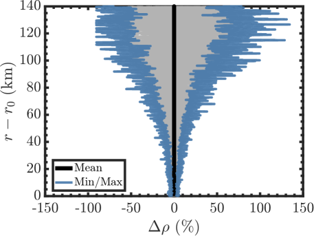
This section describes the implementation of the offline training of the neural network. It is important to highlight that various implementations can be employed for the neural network, as this network is only a starting point for the online estimation portion. To generate the training data, as previously described, a least squares exponential fit was applied to multiple Mars-GRAM profiles. Figure 1 shows the Mars-GRAM profiles used for the implementation of the neural network. To generate these profiles, the density and wind random perturbations were set to 1, representing a standard deviation in the range of 2% to 45% of the unperturbed mean.

Figure 1: Altitude as a function of the density variation for the Mars-GRAM profiles generated. The gray lines show the different atmospheric profiles.

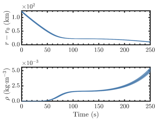
Using this exponential fit, 1000 different entry trajectories were simulated based on the dynamic equations outlined in Section 2.1. Each trajectory was initialized with distinct initial conditions, and data on atmospheric density and planet-centric radius were recorded at 0.5-second intervals during the simulations. The trajectories were propagated for 250 seconds reaching an altitude of approximately 11 kilometers above the Martian surface, a typical point marking the end of the entry phase [10]. Figure 2 shows different propagated trajectories that use different initial conditions coupled with the exponential fit for the density.

Figure 2: Altitude as a function of time (top) and density as obtained from the least squares exponential fit (bottom).

To train the neural network, a method similar to that introduced by Amato and McMahon [18] was adopted. To facilitate the training process, the output data, which represents atmospheric density, was transformed using the equation,

$$\varrho_{k}=\sqrt{\mathcal{B}-\log_{10}\rho_{k}},$$ (29)

where $\mathcal{B}$ is a shifting factor ensuring that the argument of the square root is always positive. For this work, $\mathcal{B}=0$ since the atmospheric density is consistently expressed in SI base units, ensuring that the argument of the square root is always non-negative. To assess the possibility of overfitting, a train/validation split on the data was conducted. Both the training input and output data were normalized, following the transformations,

$$i_{k} =\frac{r_{k}-\bar{r}}{\sigma_{r}},$$ (30)

$$o_{k} =\frac{\varrho_{k}-\bar{\varrho}}{\sigma_{\varrho}}.$$ (31)

where $i_{k}$ is the input to the network and $o_{k}$ represents the output. Here, $\bar{r}$ represents the mean of all training input data, $\sigma_{r}$ is the associated standard deviation, $\bar{\varrho}$ is the mean of all training output data, and $\sigma_{\varrho}$ is the associated standard deviation. With the normalized training data, a simple feed-forward network with one hidden layer with 100 neurons, and using $\tanh$ as the activation function was trained. The network was trained for 1000 epochs using Adam as the optimizer with a varying learning rate ranging from $l_{r_{\min}}=10^{-6}$ to $l_{r_{\max}}=10^{-2}$. Figure 3 illustrates the procedure for estimating atmospheric density based on the planet-centric radius using the trained neural network. The planet-centric radius ($r_{k}$) is first normalized, and this normalized input ($i_{k}$) is fed into the neural network. Subsequently, the output ($o_{k}$) is unnormalized to derive the transformed density ($\varrho_{k}$), and the density ($\rho_{k}$) is computed using the inverse mapping. The network operations are given by:

$$\bm{a}_{k} =\tanh\left\{W^{(i)}{i}_{k}+\bm{b}^{(i)}_{k}\right\},$$ (32)

$$\bm{o}_{k} =W^{(o)}\bm{a}_{k}+\bm{b}^{(o)}_{k},$$ (33)

where $\bm{a}_{k}\in\mathbb{R}^{100}$ are the neurons in the hidden layer, $W^{(i)}\in\mathbb{R}^{100\times 1}$ is the vector of weights for the first layer, $i_{k}\in\mathbb{R}$ represents the input and $\bm{b}^{(i)}_{k}\in\mathbb{R}^{100}$ are the biases for the first layer. Similarly, $o_{k}\in\mathbb{R}$ is the output of the network, and $W^{(o)}\in\mathbb{R}^{1\times 100}$ and $\bm{b}^{(o)}_{k}\in\mathbb{R}$ are the weights and biases for the output layer, respectively.

Figure 3: Network architecture used to estimate the atmospheric density from the planet-centric radius.

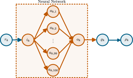
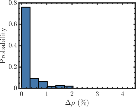
Figure 4 displays the percentage error between the estimated density from the trained neural network and the actual density in the validation set. As it can be seen, the network accurately predicts the density, as most errors are less than 1%, suggesting a good fit to the exponential model. It is important to note that the accuracy of this network is not crucial for the proposed approach. The network is expected to perform poorly on real atmospheric density profiles, which is why the weights and biases will be updated online to adapt to a higher fidelity density model. However, achieving a good fit to an exponential model is desirable.

Figure 4: Probability histogram of the relative error between the predicted density from the trained neural network and the density in the validation set.

4.2 Online estimation

Once the neural network has been trained, an online adaptation scheme can be applied. For this work, the state to be estimated is defined as:

$$\bm{x}=\left[r\,\,\phi\,\,\theta\,\,v\,\,\phi\,\,\psi\,\,B\,\,L/D\right]^{T},$$ (34)

where the inverse of the ballistic coefficient ($B$) is modeled as a random walk, employing a similar approach for modeling the lift-to-drag ratio ($L/D$) [10]. The available measurement vector is expressed as:

$$\bm{y}=\left[\tilde{\bm{a}}^{b}\,\,\tilde{q}\,\,\tilde{\dot{Q}}_{s}\right].$$ (35)

To simplify notation, the dynamics and measurement models are defined as:

$$\dot{\bm{x}} =f(\bm{x},\rho),$$ (36)

$$\bm{y}_{k} =h\left(\bm{x}_{k},\rho_{k}\right)+\bm{\eta_{k}},$$ (37)

where $f$ are the dynamics presented in section 2.1, $h$ refers to the measurement model in section 2.2, $\rho$ is the atmospheric density and $\bm{\eta_{k}}$ represents measurement noise. Process noise is modeled in the solution of the dynamics,

$$\bm{x}_{k}=F\left(\bm{x}_{k-1},\rho_{k-1}\right)+\bm{q}_{k-1}$$ (38)

where $F$ is the flow of (36) and $\bm{q}_{k-1}$ is the process noise. For this scenario, the selected online estimator is the Unscented Schmidt-Kalman filter (USKF) [33, 34]. The USKF is a linear update filter known for its robustness in handling nonlinear dynamics and measurements. This choice eliminates the need for partial derivatives both during time propagation and measurement updates, which can otherwise lead to computational slowdown as the neural network is being used to approximate the density, thus requiring the need of more complicated partial derivatives. Additionally, this filter incorporates a consider analysis to account for the uncertainty in the atmospheric density estimates, as this quantity is not part of the filter’s state space.

4.2.1 Time propagation

Each iteration starts from the previous time posterior estimate of the state $\hat{\bm{x}}^{+}_{a,k-1}$ and covariance $P^{+}_{a,k-1}$, where both the estimate and covariance are augmented to include the consider parameter,

$$\hat{\bm{x}}^{+}_{a,k-1}=\begin{bmatrix}\hat{\bm{x}}^{+\mathrm{T}}_{k-1}&\hat{\bm{c}}^{+}_{k-1}\end{bmatrix}^{\mathrm{T}},$$ (39)

$$P^{+}_{a,k-1}=\begin{bmatrix}P^{+}_{k-1}&C^{+}_{k-1}\\ \left(C^{+}_{k-1}\right)^{\mathrm{T}}&P^{+}_{c,k-1}\end{bmatrix},$$ (40)

where the initial value $P^{+}_{c,0}$ is user-defined (note that $\hat{\bm{c}}^{+}_{0}=1$ and $C^{+}_{0}=0_{n_{x}\times 1}$). With these augmented state and covariance, a set of posterior estimates is built by calculating the associated sigma points [35],

$$\bm{\mathcal{X}}^{(0)} =\hat{\bm{x}}^{+}_{a,k-1},$$ (41)

$$\bm{\mathcal{X}}^{(i)} =\hat{\bm{x}}^{+}_{a,k-1}+\left(\sqrt{L+\lambda P^{+}_{a,k-1}}\right)^{(i)},\hskip 10.00002pti=1,\cdots,L,$$ (42)

$$\bm{\mathcal{X}}^{(i)} =\hat{\bm{x}}^{+}_{a,k-1}-\left(\sqrt{L+\lambda P^{+}_{a,k-1}}\right)^{(i)},\hskip 10.00002pti=L+1,\cdots,2L,$$ (43)

resulting in a set of $2L+1$ samples. The scaling parameter $\lambda$ is defined as $\lambda=\alpha^{2}\left(L+\kappa\right)-L$, where $\alpha$ and $\kappa$ are secondary scaling parameters and $L=n_{x}+1$. The superscript $(i)$ denotes the $i$-th column of the matrix in parenthesis. The parameter $\alpha$ controls the spread of points around $\hat{\bm{x}}^{+}_{a,k-1}$ and is typically set to a small positive value ($10^{-4}\leq\alpha\leq 1$), and $\kappa$ is usually chosen as $3-L$ [35]. The set of posterior estimates at time step $k-1$ is then given by:

$${\hat{\bm{\mathcal{X}}}}^{+(i)}_{k-1} =\bm{\mathcal{X}}^{(i)}(1:n_{x}),$$ (44)

where $\bm{\mathcal{X}}^{(i)}(a:b)$ represents Matlab notation. After calculating the sigma points, these can be propagated to the next time step by integrating the dynamics and using the trained neural network to estimate the density. With $F(\bm{x},\rho)$ representing the flow of $f(\bm{x},\rho)$ and modeling the consider parameter as an exponentially correlated random variable (ECRV) [36] centered at one, the states are propagated by (note that the operator $\mathcal{N}\!\mathcal{N}\left(\cdot\right)$ handles the normalization and transformation steps):

$$\bm{\hat{\mathcal{X}}}^{-(i)}_{k} =F\left({\hat{\bm{\mathcal{X}}}}^{+(i)}_{k-1},\mathcal{P}^{(i)}_{k-1}\right),$$ (45)

$$\mathcal{P}^{(i)}_{k-1} =\hat{\bm{\mathcal{X}}}^{+(i)}_{k-1}(n_{x}+1)\cdot\mathcal{N}\!\mathcal{N}\left(\hat{\bm{\mathcal{X}}}^{+(i)}_{k-1}(1),\bm{\xi}_{k-1}\right),$$ (46)

where $\hat{\bm{\mathcal{X}}}^{+(i)}_{k-1}(n_{x}+1)$ is the consider parameter at each sigma point, $\hat{\bm{\mathcal{X}}}^{+(i)}_{k-1}(1)$ is the estimated planet-centric radius at each sigma points and $\bm{\xi}_{k-1}$ are the current weights and biases of the neural network. Note that the consider parameter is dispersing the solution of the neural network to account for the uncertainty in the atmospheric density estimate. With the propagated sigma points, a prior estimate and covariance can be calculated by a weighted sum, such that:

$$\hat{\bm{x}}^{-}_{a,k} =\sum_{i=0}^{2L}w_{m}^{(i)}\hat{\bm{\mathcal{X}}}^{-(i)}_{k},$$ (47)

$$P^{-}_{a,k} =\sum_{i=0}^{2L}w_{c}^{(i)}\left[\hat{\bm{\mathcal{X}}}^{-(i)}_{k}-\hat{\bm{x}}^{-}_{k}\right]\left[\hat{\bm{\mathcal{X}}}^{-(i)}_{k}-\hat{\bm{x}}^{-}_{k}\right]^{\mathrm{T}}+Q_{a,k-1},$$ (48)

where the weights are given by [37]:

$$w_{m}^{(0)} =\frac{\lambda}{L+\lambda},$$ (49)

$$w_{c}^{(0)} =\frac{\lambda}{L+\lambda}+1-\alpha^{2}+\beta,$$ (50)

$$w_{m}^{(i)} =w_{c}^{(i)}=\frac{1}{2\left(L+\lambda\right)},\hskip 15.00002pti=1,...,2L,$$ (51)

and the augmented process noise covariance is defined as:

$$Q_{a,k-1}=\begin{bmatrix}Q_{k-1}&0_{n_{x}\times 1}\\ 0_{1\times n_{x}}&Q_{c,k-1}\end{bmatrix},$$ (52)

with $Q_{c,k-1}=\left(1-\exp\left\{-2\Delta t_{k}/\tau\right\}\right)P_{ss}$, where $\Delta t_{k}$ is the propagation interval, $\tau$ is the time constant of the ECRV and $P_{ss}$ is the steady-state covariance of this variable. The constant $\beta$ is used to incorporate prior knowledge of the probability distribution. Under the assumption of a scalar, Gaussian prior distribution $\beta=2$ is usually regarded as optimal since it can cancel second-order error terms [37]. From the augmented state and covariance, the estimation state and its covariance can be retrieved by selecting the first $n_{x}$ elements of the resulting vector and the $n_{x}$ by $n_{x}$ upper block of the resulting matrix.

4.2.2 Maximum Likelihood optimization

Once a measurement ($\bm{y}_{k}$) is obtained, a loss function is constructed using the measurement log likelihood,

$$\mathcal{L}\left(\xi_{k-1}\right) =\left[\bm{y}_{k}-h\left(\hat{\bm{x}}^{-}_{k},\hat{\rho}_{k-1}\right)\right]^{\mathrm{T}}R^{-1}\left[\bm{y}_{k}-h\left(\hat{\bm{x}}^{-}_{k},\hat{\rho}_{k-1}\right)\right],$$ (53)

$$\hat{\rho}_{k-1} =\mathcal{N}\!\mathcal{N}\left(\hat{\bm{x}}^{-}_{k}(1),\bm{\xi}_{k-1}\right).$$ (54)

This loss function highlights the fact that the adaptation is performed in a nonlinear fashion with respect to the measurement, as opposed to the previous augmentation approaches described in section 3. Thus, a minimization problem can be constructed, where,

$$\bm{\xi}_{k}=\arg\min_{\xi_{k-1}}\mathcal{L}\left(\xi_{k-1}\right).$$ (55)

When dealing with non-convex problems, fine-tuning the learning rate in traditional optimization algorithms (such as Newton-Raphson) can present challenges and may lead to divergence issues. Instead, we propose the use of automatic differentiation and stochastic optimizers to address the minimization problem in (55). Given that this problem pertains to the optimization of the weights and biases of a neural network, back-propagation (also known as adjoint-mode differentiation) can be employed to compute precise gradients (up to floating-point precision). Furthermore, the adaptive and stochastic optimization capabilities offered by the Adam optimizer [32] can be leveraged to minimize the loss function. A notable advantage of using the Adam optimizer is its ability to incorporate memory of previous gradients from earlier time steps, thereby assisting in the fine-tuning of the adaptive learning rate within the optimizer. Starting from an initial gradient $\nabla_{\bm{\xi}_{k-1}}\mathcal{L}$, an initial moving average of the gradient $\bar{\nabla}_{k-1}$, and an initial moving average of the squared gradient $\left(\bar{\nabla}_{k-1}\right)^{2}$, where the notation $\left(\cdot\right)^{2}$ indicates element-wise square, Adam iteratively updates the network parameters as follows. First the moving average of the gradient and the gradient squared are updated,

$$\bar{\nabla}_{k-1}^{\star} =\beta_{1}\bar{\nabla}_{k-1}+\left(1-\beta_{1}\right)\nabla_{\bm{\xi}_{k-1}}\mathcal{L},$$ (56)

$$\left(\bar{\nabla}_{k-1}^{\star}\right)^{2} =\beta_{2}\left(\bar{\nabla}_{k-1}\right)^{2}+\left(1-\beta_{2}\right)\left(\nabla_{\bm{\xi}_{k-1}}\mathcal{L}\right)^{2},$$ (57)

where $\beta_{1}$ and $\beta_{2}$ are exponential decay rates of the moving averages being estimated. Once these two estimates are obtained, the network parameters are updated using the following equation:

$$\bm{\xi}_{k-1}^{\star}=\bm{\xi}_{k-1}-\alpha_{\mathcal{L}}\left({\bar{\nabla}_{k-1}^{\star}}\Big{/}\left[{\sqrt{\left(\bar{\nabla}_{k-1}^{\star}\right)^{2}}+\epsilon}\right]\right).$$ (58)

Here, $\alpha_{\mathcal{L}}$ represents the step size, and $\epsilon$ is a small constant used to prevent numerical overflow. This process repeats until a convergence criterion is met. When a convergence criterion is satisfied, the updated network parameters and moving averages are saved for the measurement update and the next iteration. Thus, upon reaching convergence,

$$\bar{\nabla}_{k} =\bar{\nabla}_{k-1}^{\star},$$ (59)

$$\left(\bar{\nabla}_{k}\right)^{2} =\left(\bar{\nabla}_{k-1}^{\star}\right)^{2},$$ (60)

$$\bm{\xi}_{k} =\bm{\xi}_{k-1}^{\star}.$$ (61)

For this work, the moving average of the gradient was initialized to zero, and the square of the gradient was initialized to the current gradient squared. Additionally, the moving averages were not corrected for the initialization bias. These design strategies were informed by the performance of the algorithm when deployed online in different filtering tests. In practice, the maximization step is only performed if the initially evaluated loss exceeds a predetermined threshold ($\mathcal{T}$). This helps alleviate the computational burden of the online filter and leads to less noisy outcomes. Algorithm 1 provides a comprehensive overview of the maximum likelihood optimization step. In this algorithm, a maximum patience value $(p_{\max})$ is defined to prevent the degradation of the neural network in the event of encountering unfavorable gradients.

Algorithm 1 Maximum Likelihood optimization

1:$\hat{\bm{x}}^{-}_{a,k},P^{-}_{a,k},\bm{\xi}_{k-1},\bar{\nabla}_{k-1},\left(\bar{\nabla}_{k-1}\right)^{2},\alpha_{\mathcal{L}},\beta_{1},\beta_{2},p_{\max},\mathcal{T}$

2:$\bm{\xi}_{k},\bar{\nabla}_{k},\left(\bar{\nabla}_{k}\right)^{2}$

3:Calculate initial loss: $\mathcal{L}(\bm{\xi}_{k-1})$

4:Initialize patience: $p=0$

5:while $\mathcal{L}(\bm{\xi}_{k-1})$ < $\mathcal{T}$ do

6:     Apply back-propagation to obtain the gradients: $\nabla_{\bm{\xi}_{k-1}}\mathcal{L}$

7:     Use Adam to obtain new parameters, average gradient and average gradient squared:

8:     $\left[\bm{\xi}^{\star}_{k-1},\bar{\nabla}^{\star}_{k-1},\left(\bar{\nabla}^{\star}_{k-1}\right)^{2}\right]$ = Adam$\left[\bm{\xi}_{k-1},\nabla_{\bm{\xi}_{k-1}}\mathcal{L},\bar{\nabla}_{k-1},\left(\bar{\nabla}_{k-1}\right)^{2},\alpha_{\mathcal{L}},\beta_{1},\beta_{2}\right]$

9:     Evaluate new loss: $\mathcal{L}(\bm{\xi}^{\star}_{k-1})$

10:     if $\mathcal{L}(\bm{\xi}^{\star}_{k-1})$ < $\mathcal{L}(\bm{\xi}_{k-1})$ then

11:         Update adapted parameters: $\bm{\xi}_{k-1}\leftarrow\bm{\xi}^{\star}_{k-1}$

12:         Update Adam parameters: $\left(\bar{\nabla}_{k-1},\left(\bar{\nabla}_{k-1}\right)^{2}\right)\leftarrow\left(\bar{\nabla}_{k-1}^{\star},\left(\bar{\nabla}^{\star}_{k-1}\right)^{2}\right)$

13:         Update loss: $\mathcal{L}(\bm{\xi}_{k-1})\leftarrow\mathcal{L}(\bm{\xi}^{\star}_{k-1})$

14:     else

15:         Update patience: $p=p+1$

16:     end if

17:     if $p=p_{\max}$ then

18:         break

19:     end if

20:end while

21:Save adapted parameters: $\bm{\xi}_{k}\leftarrow\bm{\xi}_{k-1}$

22:Save Adam parameters: $\left(\bar{\nabla}_{k},\left(\bar{\nabla}_{k}\right)^{2}\right)\leftarrow\left(\bar{\nabla}_{k-1},\left(\bar{\nabla}_{k-1}\right)^{2}\right)$

4.2.3 Measurement update

Once the adapted weights and biases of the network have been obtained, the measurement update can be performed. To do this, sigma points are calculated around the prior estimate by using the propagated state and covariance and using the same approach as in equations (41)-(43). With the set of prior sigma points, a set of expected measurements is calculated by using the measurement model and the adapted weights and biases of the network,

$$\hat{\mathcal{Y}}^{(i)}_{k} =h\left(\hat{\bm{\mathcal{X}}}^{-(i)}_{k},\mathcal{P}^{(i)}_{k}\right),$$ (62)

$$\mathcal{P}^{(i)}_{k} =\hat{\bm{\mathcal{X}}}^{-(i)}_{k}(n_{x}+1)\cdot\mathcal{N}\!\mathcal{N}\left(\hat{\bm{\mathcal{X}}}^{-(i)}_{k}(1),\bm{\xi}_{k}\right).$$ (63)

Notice again that the atmospheric density estimate obtained from the network is slightly perturbed by the consider parameter for each sigma point in order to account for uncertainties. With the set of expected measurements, the predicted mean, its covariance and cross-covariance with the state can be calculated to perform a Kalman update. Using a similar weighted sum as in the time propagation,

$$\hat{\bm{y}}_{k} =\sum_{i=0}^{2L}w_{m}^{(i)}\hat{\mathcal{Y}}^{(i)}_{k},$$ (64)

$$P_{yy,k} =\sum_{i=0}^{2L}w_{c}^{(i)}\left[\hat{\bm{\mathcal{Y}}}^{(i)}_{k}-\hat{\bm{y}}_{k}\right]\left[\hat{\bm{\mathcal{Y}}}^{(i)}_{k}-\hat{\bm{y}}_{k}\right]^{\mathrm{T}}+R_{k},$$ (65)

$$P_{x_{a}y,k} =\sum_{i=0}^{2L}w_{c}^{(i)}\left[\hat{\bm{\mathcal{X}}}^{-(i)}_{k}-\hat{\bm{x}}^{-}_{k}\right]\left[\hat{\bm{\mathcal{Y}}}^{(i)}_{k}-\hat{\bm{y}}_{k}\right]^{\mathrm{T}},$$ (66)

where $R_{k}$ is the measurement noise covariance, and the weights are calculated using the same equations as in the time propagation. It is important to note that for the measurement update, the constants $\alpha,\beta$ and $\kappa$ do not necessarily have to be the same as in the time propagation step. With the obtained matrices, a Kalman gain is calculated,

$$K_{k}=P_{x_{a}y,k}P_{yy,k}^{-1}=\begin{bmatrix}K_{x,k}\\ K_{c,k}\end{bmatrix}$$ (67)

Finally, a Kalman update can be performed to obtain the posterior estimate and covariance, such that:

$$\hat{\bm{x}}^{+}_{a,k} =\hat{\bm{x}}^{-}_{a,k}+\begin{bmatrix}K_{x,k}\\ 0\end{bmatrix}\left(\bm{y_{k}}-\hat{\bm{y}}_{k}\right),$$ (68)

$$P^{+}_{a,k} =P^{-}_{a,k}-\begin{bmatrix}K_{x,k}P_{yy,k}K_{x,k}^{\mathrm{T}}&K_{x,k}P_{yy,k}K_{c,k}^{\mathrm{T}}\\ K_{c,k}P_{yy,k}K_{x,k}^{\mathrm{T}}&0\end{bmatrix}.$$ (69)

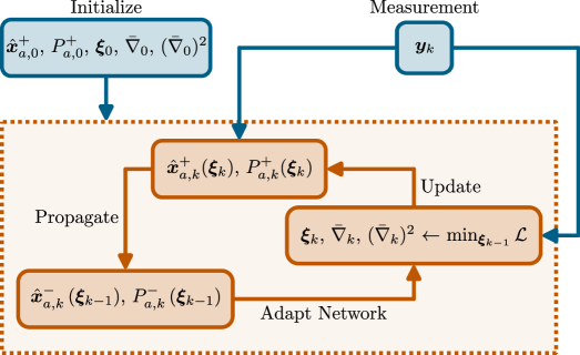
Just as with the time propagation, from the augmented state and covariance, the estimation state and its covariance can be retrieved by selecting the first $n_{x}$ elements of the resulting vector and the $n_{x}$ by $n_{x}$ upper block of the resulting matrix. It is important to note that the consider parameter and its associated covariance are not updated in this filter. A summary of the complete online estimation scheme is presented in Fig. 5. First, the neural network is trained offline to obtain the initial weights and biases ($\bm{\xi}_{0}$) and the initial Adam parameters ($\bar{\nabla}_{0}$, $(\bar{\nabla}_{0})^{2}$), state and covariance ($\hat{\bm{x}}^{+}_{a,0}$, $P^{+}_{a,0}$) are set as the starting point ($k-1$). Then, the state and covariance are propagated ($\hat{\bm{x}}^{-}_{a,k}$, $P^{-}_{a,k}$) using the current network. Once the measurement is obtained $(\bm{y}_{k})$, the loss function $(\mathcal{L})$ is minimized using Adam and the network ($\bm{\xi}_{k}$) and optimizer parameters ($\bar{\nabla}_{k}$, $(\bar{\nabla}_{k})^{2}$) are adapted. Finally, the state and covariance are updated ($\hat{\bm{x}}^{+}_{a,k}$, $P^{+}_{a,k}$) using the adapted network.

Figure 5: Flowchart of the density adaptation scheme.

5 Results and Discussion

To assess the density adaptation scheme, a comprehensive Monte Carlo testing approach was employed. This involved conducting 500 Monte Carlo runs to thoroughly evaluate the robustness and performance of the algorithms presented. Each true trajectory was simulated using an independent and distinct Mars-GRAM density trajectory from the previously mentioned set, as depicted in Fig. 1. Given that Mars-GRAM trajectories provide density at discrete altitudes, trajectory points were interpolated using a cubic spline to determine density values at the query altitude.

All trajectories were initialized with the entry conditions for the Mars Science Laboratory (MSL), outlined in Table 1. This implies simulating potential MSL entry trajectories for various densities the vehicle might encounter. It is crucial to note that these trajectories are simulated in an open-loop fashion, meaning that no bank control is executed, as the focus of this work is solely on the navigation aspect. However, the methodology presented herein is expected to be robust to control inputs. A constant bank angle ($\sigma=0$) and a constant angle of attack ($\alpha=-17^{\circ}$) were assumed for all trajectories, based on the available initial entry conditions of the MSL.

Table 1: Entry conditions for the true trajectories

Parameter	Value	Standard Deviation (3$\sigma$)
$r_{0}$ (m) [16]	$3.5222\text{\times}{10}^{6}$	$3.2066\text{\times}{10}^{1}$
$\phi_{0}$ (deg) [16]	$-0.3919\text{\times}{10}^{1}$	$7.8100\text{\times}{10}^{-4}$
$\theta_{0}$ (deg) [16]	$1.2672\text{\times}{10}^{2}$	$3.6700\text{\times}{10}^{-4}$
$v_{0}$ (m/s) [16]	$6.0833\text{\times}{10}^{3}$	$2.6059\text{\times}{10}^{-2}$
$\gamma_{0}$ (deg) [16]	$1.5489\text{\times}{10}^{1}$	$4.0000\text{\times}{10}^{-4}$
$\psi_{0}$ (deg) [16]	$9.3206\text{\times}{10}^{1}$	$2.6800\text{\times}{10}^{-4}$
$B_{0}$ (m2/kg)	$7.1000\text{\times}{10}^{-3}$ [38]	$4.8000\text{\times}{10}^{-3}$ [10]
$L_{0}/D_{0}$ (n.d.)	$2.4000\text{\times}{10}^{-1}$ [38]	$1.5178\text{\times}{10}^{-1}$ [10]

The true dynamics were propagated for 350 seconds, reaching altitudes close to 11 kilometers. In addition, the dynamics were propagated with additive zero-mean Gaussian process noise and measurements were calculated using the true state with additive zero-mean Gaussian noise as well. Both the process noise and measurement noise were assumed to be white and uncorrelated with any additional sources of error. For this work, all sensors were sampled at a uniform frequency of 4 Hz. Tables 2 and 3 provide the statistics used for the process and measurement noise, respectively. The consider parameter was modeled as an ECRV with $\tau=5$ and $P_{ss}=$1\text{\times}{10}^{-3}$$.

Table 2: Process noise statistics

Parameter	Standard Deviation ($3$$\sigma$)
$r$ (m)	-
$\phi$ (deg)	-
$\theta$ (deg)	-
$v$ (m/s)	$3\text{\times}{10}^{-1}$
$\gamma$ (deg)	$4\text{\times}{10}^{-6}$
$\psi$ (deg)	$4\text{\times}{10}^{-7}$
$B$ (m2/kg)	$1\text{\times}{10}^{-5}$
$L/D$ (n.d.)	$3\text{\times}{10}^{-5}$

Table 3: Measurement noise statistics

Parameter	Standard Deviation ($3$$\sigma$)
$\tilde{\bm{a}}^{b}$ $(\mu g)$ [24]	$1\text{\times}{10}^{2}$
$\tilde{q}$ (% of reading) [20]	$1$
$\tilde{\dot{Q}}_{s}$ (% of reading)	$1$

To evaluate the effectiveness of the density adaptation scheme, three filters were implemented for a comparative analysis. The first filter, labeled UKF-CM (CM for covariance matching), uses the least squares exponential fit to the Mars-GRAM trajectories for density estimation and implements a covariance matching technique to estimate the process noise covariance as defined in (20), with a moving window of 5 time steps, following the approach presented in [14]. Since the estimate of the process noise covariance may become negative definite, the diagonal elements are always reset to the absolute value of their estimates [15]. This filter is implemented using an unscented Kalman filter [35] without consider analysis, since the tuning of the process noise covariance is expected to account for the uncertainty in the density. The second filter, denoted as UKF-AC (AC for augmentation and correction), augments the estimation state to compute a correction to a nominal profile as defined in (24) and (25). The nominal profile is derived from the least squares exponential fit to the Mars-GRAM trajectories. This filter is implemented using a UKF without consider analysis as the augmentation of the state mirrors the consider approach, with the distinction that the consider parameter and covariance are updated. The third filter, referred to as USKF-NN (NN stands for neural network), adheres to the framework detailed in Section 4. The chosen filters are intended to enable a meaningful comparison of similar strategies, as each solution uses identical base state spaces and measurements. This approach ensures a fair assessment of the strategies under consideration.

The parameters used for the maximum likelihood optimization are summarized in Table 4. It is important to note that the learning rate within Adam is dynamically lowered with respect to the time step ($k$), as higher gradients are expected when the vehicle reaches maximum dynamic pressure. All filters use the same values for the parameters in the unscented transform, where $\alpha=1$, $\kappa=3-L$, and $\beta=2$. The initial filter state is sampled from a Gaussian distribution for each Monte Carlo simulation, with the true state as its mean and a diagonal covariance matrix following the uncertainty values as described in Table 1.

Table 4: Maximum Likelihood parameters used in the USKF-NN

Parameter	Value
$\beta_{1}$	0.1
$\beta_{2}$	0.9
$p_{\max}$	1
$\alpha_{\mathcal{L}}$	$0.01/k$

To quantify the accuracy of each filter, the time-averaged mean absolute error (MAE) is used, defined as:

$$\mathrm{MAE}_{i}=\frac{1}{N_{k}}\sum_{k=1}^{N_{k}}\sum_{j=1}^{N_{m}}\frac{\left|x_{i}(k)^{(j)}-\hat{x}^{+}_{i}(k)^{(j)}\right|}{N_{m}},$$ (70)

where $N_{k}$ is total number of discrete steps in each simulation, $N_{m}$ is the number of Monte Carlo simulations, $x_{i}(k)^{(j)}$ is the $i$-th true state and $\hat{x}^{+}_{i}(k)^{(j)}$ is the $i$-th posterior estimate. Table 5 presents the time-averaged MAE obtained for each state using the three studied filtering strategies. The USKF-NN consistently outperforms both the UKF-CM and the UKF-AC, demonstrating significantly lower estimation errors across all states. This improvement serves as evidence that the newly introduced adaptation scheme can outperform previous strategies. Notably, the UKF-AC obtains a lower estimation error than the UKF-CM for most of the estimated states, attributed to the adaptive density scheme employed in the UKF-AC.

Table 5: Time-averaged mean absolute error for the three filtering strategies

Parameter	UKF-CM	UKF-AC	USKF-NN
${r}$ (m)	$2.9360\text{\times}{10}^{03}$	$3.9804\text{\times}{10}^{03}$	$6.3226\text{\times}{10}^{01}$
${\phi}$ (deg)	$1.8868\text{\times}{10}^{-01}$	$8.0763\text{\times}{10}^{-03}$	$6.1745\text{\times}{10}^{-04}$
${\theta}$ (deg)	$1.0707\text{\times}{10}^{-02}$	$4.8417\text{\times}{10}^{-04}$	$1.5682\text{\times}{10}^{-04}$
${v}$ (m/s)	$2.0236\text{\times}{10}^{01}$	$0.6606\text{\times}{10}^{01}$	$5.5082\text{\times}{10}^{-01}$
${\gamma}$ (deg)	$3.9092\text{\times}{10}^{01}$	$7.2287\text{\times}{10}^{-01}$	$1.2009\text{\times}{10}^{-02}$
${\psi}$ (deg)	$1.8280\text{\times}{10}^{-03}$	$1.1586\text{\times}{10}^{-03}$	$1.1572\text{\times}{10}^{-03}$
${B}$ (m2/kg)	$8.2719\text{\times}{10}^{-05}$	$1.8397\text{\times}{10}^{-04}$	$4.4882\text{\times}{10}^{-05}$
${L}/D$ (n.d.)	$1.9518\text{\times}{10}^{-03}$	$1.8588\text{\times}{10}^{-03}$	$1.8434\text{\times}{10}^{-03}$

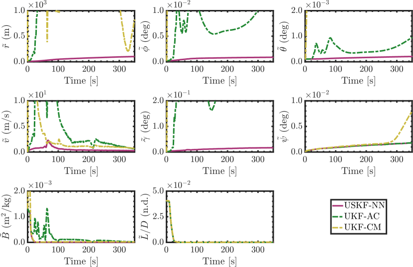
Figure 6 displays the mean absolute error as a function of time for each estimation state and each of the three filtering strategies. The USKF-NN outperforms every other filter for all considered time steps, achieving the lowest estimation error across all states. In contrast, the UKF-AC and the UKF-CM show high estimation errors, particularly in states affected by the atmospheric density. The states not dependent on the density for dynamic propagation, such as the heading angle (since the bank angle is set to zero), the inverse of the ballistic coefficient, and the lift-to-drag ratio, have similar estimation errors across all the filtering strategies. There is an exception for the heading angle in UKF-CM, where the estimation error tends to diverge at the end of the trajectory. This figure highlights the significant improvement in accuracy achieved when the onboard atmospheric density is adapted following the maximum likelihood approach, especially in states whose dynamic propagation is influenced by the atmospheric conditions.

Figure 6: Mean absolute error for each state obtained with each of the three filtering strategies.

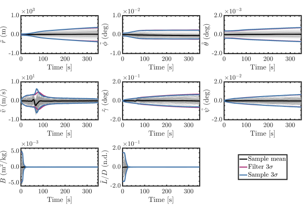
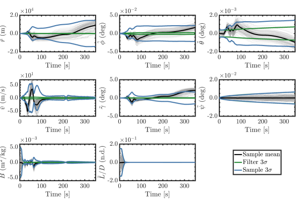
The consistency improvement of the USKF-NN over the other filtering strategies can be further analyzed in Fig. 7 and Fig. 8. These figures show the error plots obtained with the USKF-NN and the UKF-AC, respectively. The error plots for the UKF-CM are not presented, as they were not considered particularly informative for the analysis since the filter is highly inconsistent. The estimates obtained with the USKF-NN exhibit minimal bias as the estimation error remains close to zero mean for all states. In addition, the predicted covariance of this filter closely aligns with the sample variance of the errors, showing that the USKF-NN is a consistent filter for this scenario. It is important to note that the estimates for the velocity struggle to be zero mean when maximum dynamic pressure is reached (although the covariance of the filter accounts for this error), but the filter quickly recovers maintaining unbiased estimates for the remainder of the flight. Conversely, the UKF-AC struggles to obtain unbiased estimates as the errors are highly biased (the estimates for the heading angle remain unbiased since $\sigma=0$, thus making the dynamic propagation of this state independent of the density). The disparity between the true atmospheric density and the onboard estimated density can rapidly introduce bias into the estimates, explaining the sub-optimal performance of the UKF-AC in this regard. This filter also struggles in capturing the uncertainty of its estimates as the predicted filter covariance does not match the variance of the estimation errors.

With the measurement setup used in this work, the estimated states are not entirely observable (A more comprehensive observability analysis is detailed in [39]). Consequently, only the velocity and aerodynamic parameters emerge as truly observable states, as seen in Fig. 7. Nevertheless, the USKF-NN achieves consistent results that can potentially be improved as more measurements become available in the descent and landing phases. The results from the UKF-AC are uninformative and it would be difficult to recuperate the estimates once more measurements are available.

Figure 7: Estimation error as a function of time for the results obtained with the USKF-NN. The gray lines show different Monte Carlo trajectories.

Given the comparable strategies employed by the UKF-AC and the USKF-NN, both incorporating online adaptation of the atmospheric density model, it is important to quantify the error in the density estimates associated with this online adaptation. To measure the difference between the true atmospheric density and the estimate generated by each filter, the time-averaged mean absolute percentage error (MAPE) is used. In this work, this metric is defined as follows:

$$\mathrm{MAPE}=\frac{1}{N_{k}}\sum_{k=1}^{N_{k}}\frac{1}{N_{m}}\sum_{j=1}^{N_{m}}\frac{\left|\rho(k)^{(j)}-\hat{\rho}(k)^{(j)}\right|}{\rho(k)^{(j)}},$$ (71)

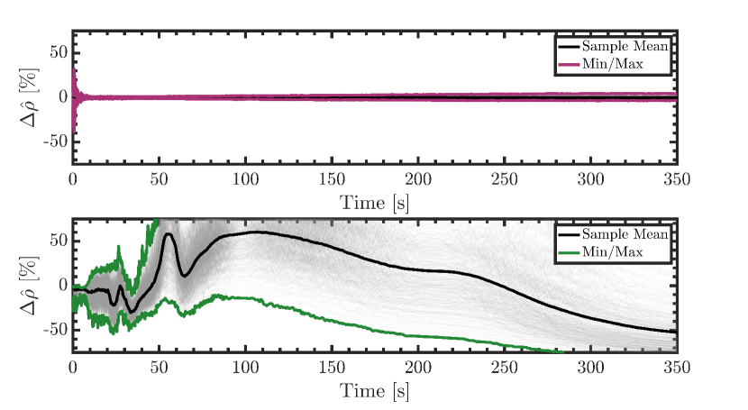
where $N_{k}$ is total number of discrete steps in each simulation, $N_{m}$ is the number of Monte Carlo simulations, $\rho(k)^{(j)}$ is the true atmospheric density and $\hat{\rho}(k)^{(j)}$ is the estimated density. Table 6 displays the time-averaged MAPE of the density estimates for both the UKF-AC and USKF-NN. The estimates derived from the USKF-NN significantly outperform those from the UKF-AC, evidenced by the substantial difference in MAPE. The USKF-NN excels over the UKF-AC by nearly two orders of magnitude, representing a smaller error in relation to the true density.

Table 6: Time-averaged mean absolute percentage error of the estimated densities

Filter	MAPE (%)
UKF-AC	$38.3435$
USKF-NN	$0.6734$

Figure 8: Estimation error as a function of time for the results obtained with the UKF-AC. The gray lines show different Monte Carlo trajectories. Note that, for improved readability, the $\bm{y}$-scale differs from that in Fig. 7 for variables $\tilde{r}$, $\tilde{\theta}$, $\tilde{v}$, and $\tilde{\gamma}$.

The difference in density estimates between these two filters can be further analyzed in Fig. 9, which depicts the MAPE as a function of time for both solutions. The figure clearly illustrates the superior performance of the USKF-NN over the UKF-AC. The density estimates generated by the USKF-NN closely track the true density, exhibiting a very low percentage error. In contrast, the UKF-AC struggles to accurately follow the true density, resulting in relative errors that exceed the 50% mark. As previously mentioned, the USKF-NN adapts the density model in a nonlinear fashion with respect to the measurement, while the UKF-AC employs a linear update to this model. The discernible difference in error between the USKF-NN and the UKF-AC explains the improvement in estimated states, as depicted in Fig. 7, highlighting the performance gains achieved through this nonlinear adaptation technique.

Figure 9: Mean absolute percentage error of the estimated density as a function of time for the USKF-NN (top) and the UKF-AC (bottom).

6 Conclusions

This work introduces a new approach to onboard real-time filtering for Martian entry using a neural network to estimate atmospheric density and employing a consider analysis to account for the uncertainty in this parameter. The network is trained on a simple exponential atmospheric density model, and its parameters are dynamically adapted in real-time to address any disparities between the true and estimated densities. The adaptation of the network is formulated as a maximum likelihood problem, leveraging the measurement innovations of the filter in a nonlinear fashion to identify optimal network parameters. The incorporation of a neural network enables the use of stochastic optimizers from the machine learning domain (such as Adam) within the context of the maximum likelihood adaptive estimation. Adam is highly optimized for neural networks and known for its accuracy and efficiency.

Three different filtering strategies were implemented to evaluate the effectiveness of the new adaptation scheme. An unscented Kalman filter with covariance matching, an unscented Kalman filter with density adaptation by state augmentation, and the newly presented approach were tested through a Monte Carlo analysis with different possible atmospheric profiles sampled from Mars-GRAM. The new approach outperformed the other two filters in terms of estimation error, yielding mostly unbiased and consistent estimates. Additionally, the new approach successfully adapted the onboard density model to match the atmospheric profiles provided by Mars-GRAM within an error of 0.7%.

Future work includes the incorporation of this new adaptation technique into a closed-loop simulation to evaluate the robustness of the solution to control inputs. Additionally, the modeled dynamics can be expanded to encompass the attitude of the vehicle as part of the state to leverage measurements from the gyroscope in the inertial measurement unit, potentially improving filtering performance and nonlinear adaptation.

References

- Zanetti [2007] Zanetti, R., “Advanced Navigation Algorithms for Precision Landing,” Ph.D. thesis, The University of Texas at Austin, 2007.
- Tracy et al. [2023] Tracy, K., Falcone, G., and Manchester, Z., “Robust Entry Guidance with Atmospheric Adaptation,” Proceedings of the AIAA SciTech Forum, National Harbor, MD, 2023.
- Putnam and Braun [2014] Putnam, Z. R., and Braun, R. D., “Drag-Modulation Flight-Control System Options for Planetary Aerocapture,” Journal of Spacecraft and Rockets, Vol. 51, No. 1, 2014, pp. 139–150.
- Liu et al. [2018] Liu, G., England, S. L., Lillis, R. J., Withers, P., Mahaffy, P. R., Rowland, D. E., Elrod, M., Benna, M., Kass, D. M., Janches, D., and Jakosky, B., “Thermospheric Expansion Associated With Dust Increase in the Lower Atmosphere on Mars Observed by MAVEN/NGIMS,” Geophysical Research Letters, Vol. 45, No. 7, 2018, pp. 2901–2910.
- Braun and Manning [2006] Braun, R. D., and Manning, R. M., “Mars exploration entry, descent and landing challenges,” 2006 IEEE Aerospace Conference, Big Sky, Montana, 2006.
- Lévesque [2006] Lévesque, J., “Advanced Navigation and Guidance for High-Precision Planetary Landing on Mars,” Ph.D. thesis, University of Sherbrooke, 2006.
- Zanetti and Bishop [2007] Zanetti, R., and Bishop, R., “Precision Entry Navigation Dead-Reckoning Error Analysis: Theoretical Foundations of the Discrete-Time Case,” Proceedings of the AAS/AIAA Astrodynamics Specialist Conference, Mackinac Island, MI, 2007.
- Lou et al. [2015] Lou, T., Fu, H., Zhang, Y., and Wang, Z., “Consider unobservable uncertain parameters using radio beacon navigation during Mars entry,” Advances in Space Research, Vol. 55, No. 4, 2015, pp. 1038–1050.
- Jiang et al. [2018] Jiang, X., Li, S., and Huang, X., “Radio/FADS/IMU integrated navigation for Mars entry,” Advances in Space Research, Vol. 61, No. 5, 2018, pp. 1342–1358.
- Zewge and Bang [2023] Zewge, N. S., and Bang, H., “A Distributionally Robust Fusion Framework for Autonomous Multisensor Spacecraft Navigation during Entry Phase of Mars Entry, Descent, and Landing,” Remote Sensing, Vol. 15, No. 1139, 2023.
- Marcus et al. [2022] Marcus, C., Setterfield, T., and Zanetti, R., “Variable Resolution Quadtree Mapping for Planetary Landing Using Planar Elements,” Proceedings of the AAS Guidance and Control Conference, Breckenridge, CO, 2022.
- Marcus and Zanetti [2023] Marcus, C., and Zanetti, R., “MHN-SLAM for Planetary Landing,” Proceedings of the AAS/AIAA Astrodynamics Specialist Conference, Big Sky, MT, 2023.
- Dutta et al. [2013] Dutta, S., Braun, R., Russel, R., Striepe, S., and Clark, I., “Comparison of Statistical Estimation Techniques for Mars Entry, Descent, and Landing Reconstruction,” Journal of Spacecraft and Rockets, Vol. 50, No. 6, 2013, pp. 1207–1221.
- Dutta et al. [2014] Dutta, S., Braun, R., and Karlgaard, C., “Uncertainty Quantification for Mars Entry, Descent, and Landing Reconstruction Using Adaptive Filtering,” Journal of Spacecraft and Rockets, Vol. 51, No. 3, 2014, pp. 967–977.
- Myers and Tapley [1976] Myers, K., and Tapley, B., “Adaptive Sequential Estimation with Unknown Noise Statistics,” IEEE Transactions on Automatic Control, Vol. 21, No. 4, 1976, pp. 520–523.
- Dutta and Braun [2014] Dutta, S., and Braun, R., “Statistical Entry, Descent, and Landing Performance Reconstruction of the Mars Science Laboratory,” Proceedings of the AIAA Atmospheric Flight Mechanics Conference, National Harbor, MD, 2014.
- Wagner et al. [2011] Wagner, J. J., Wilhite, A. W., Stanley, D. O., and Powell, R. W., “An Adaptive Real Time Atmospheric Prediction Algorithm for Entry Vehicles,” Proceedings of the 3rd AIAA Atmospheric Space Environments Conference, Honolulu, Hawaii, 2011.
- Amato and McMahon [2021] Amato, D., and McMahon, J. W., “Deep Learning Method for Martian Atmosphere Reconstruction,” Journal of Aerospace Information Systems, Vol. 18, 2021, pp. 728–738.
- Roelke et al. [2023] Roelke, E., McMahon, J. W., Braun, R. D., and Hattis, P. D., “Atmospheric Density Estimation Techniques for Aerocapture,” Journal of Spacecraft and Rockets, Vol. 60, 2023, pp. 942–956.
- Gazarik et al. [2008] Gazarik, M. J., Wright, M. J., Little, A., Cheatwood, F. M., Herath, J. A., Munk, M. M., Novak, F. J., and Martinez, E. R., “Overview of the MEDLI Project,” Proceedings of the 2008 IEEE Aerospace Conference, Big Sky, MT, 2008.
- Hwang et al. [2016] Hwang, H., Bose, D., White, T., Wright, H., Schoenenberger, M., Kuhl, C., Trombetta, D., Santos, J., Oishi, T., Karlgaard, C., and et al, “Mars 2020 Entry, Descent and Landing Instrumentation 2 (MEDLI2),” Proceedings of the 46th AIAA Thermophysics Conference, Washington DC, USA, 2016.
- White et al. [2022] White, T., Mahzari, M., Miller, R., Tang, C., Monk, J., Santos, J., Karlgaard, C., Alpert, H., Wright, H., and Kuhl, C., “Mars Entry Instrumentation Flight Data and Mars 2020 Entry Environments,” Proceedings of the AIAA SCITECH 2022 Forum, San Diego, CA, 2022.
- Vinh and Busemann [1980] Vinh, N., and Busemann, R., A.and Culp, Hypersonic and Planetary Entry Flight Mechanics, The University of Michigan Press, 1980.
- Braun and Manning [2007] Braun, R. D., and Manning, R. M., “Statistical Reconstruction of Mars Entry, Descent, and Landing Trajectories and Atmospheric Profiles,” Proceedings of the AIAA SPACE 2007 Conference & Exposition, Long Beach, California, 2007.
- Sutton and Randolph A. Graves [1971] Sutton, K., and Randolph A. Graves, J., “A General Stagnation-Point Convective-Heating Equation for Arbitrary Gas Mixtures,” Tech. rep., NASA Langley Research Center, 1971.
- Benito and Mease [2010] Benito, J., and Mease, K. D., “Reachable and Controllable Sets for Planetary Entry and Landing,” Journal of Guidance, Control, and Dynamics, Vol. 33, No. 3, 2010, pp. 641–654.
- Regan and Anandakrishnan [1993] Regan, F. J., and Anandakrishnan, S. M., Dynamics of Atmospheric Re-Entry, American Institute of Aeronautics and Astronautics, 1993.
- Justh [2014] Justh, H., Mars Global Reference Atmospheric Model 2010 Version: Users Guide, NASA, 2014.
- Mehra [1972] Mehra, R., “Approaches to adaptive filtering,” IEEE Transactions on Automatic Control, Vol. 17, No. 5, 1972, pp. 693–698.
- Marschke et al. [2008] Marschke, J., Crassidis, J., and Lam, Q., “Multiple Model Adaptive Estimation for Inertial Navigation During Mars Entry,” Proceedings of the AIAA/AAS Astrodynamics Specialist Conference and Exhibit, Honolulu, Hawai, 2008.
- Chu et al. [1996] Chu, Q. P., Mulder, J. A., and van Woerkom, P. T., “Modified Recursive Maximum Likelihood Adaptive Filter for Nonlinear Aircraft Flight-Path Reconstruction,” Journal of Guidance, Control and Dynamics, Vol. 19, No. 6, 1996, pp. 1285–1295.
- Kingma and Ba [2017] Kingma, D. P., and Ba, J., “Adam: A Method for Stochastic Optimization,” Proceedings of the 3rd International Conference for Learning Representations, San Diego, CA, 2017.
- Zanetti and DeMars [2013] Zanetti, R., and DeMars, K. J., “Joseph Formulation of Unscented and Quadrature Filters with Application to Consider States,” Journal of Guidance, Control, and Dynamics, Vol. 36, No. 6, 2013, pp. 1860–1864.
- Stauch and Jah [2015] Stauch, J., and Jah, M., “Unscented Schmidt–Kalman Filter Algorithm,” Journal of Guidance, Control, and Dynamics, Vol. 38, No. 1, 2015, pp. 117–123.
- Julier and Uhlmann [2004] Julier, S., and Uhlmann, J., “Unscented filtering and nonlinear estimation,” Proceedings of the IEEE, Vol. 92, No. 3, 2004, pp. 401–422.
- Zanetti and D’Souza [2013] Zanetti, R., and D’Souza, C., “Recursive Implementations of the Consider Filter,” Journal of the Astronautical Sciences, Vol. 60, No. 3, 2013, p. 672–685.
- Wan and van der Merwe [2001] Wan, E. A., and van der Merwe, R., Kalman Filtering and Neural Networks, John Wiley & Sons, Ltd, 2001.
- Way et al. [2006] Way, D. W., Powell, R. W., Chen, A., Steltzner, A. D., Martin, A. M. S., Burkhart, P. D., and Mendeck, G. F., “Mars Science Laboratory: Entry, Descent, and Landing System Performance,” 2006 IEEE Aerospace Conference, Big Sky, Montana, 2006.
- Lévesque and de Lafontaine [2007] Lévesque, J., and de Lafontaine, J., “Innovative Navigation Schemes for State and Parameter Estimation During Mars Entry,” Journal of Guidance Control and Dynamics, Vol. 30, No. 1, 2007, pp. 169–184.