Multiply Robust Estimation of Causal Effect Curves for Difference-in-Differences Designs

Abstract

Researchers commonly use difference-in-differences (DiD) designs to evaluate public policy interventions. While established methodologies exist for estimating effects in the context of binary interventions, policies often result in varied exposures across regions implementing the policy. Yet, existing approaches for incorporating continuous exposures face substantial limitations in addressing confounding variables associated with intervention status, exposure levels, and outcome trends. These limitations significantly constrain policymakers’ ability to fully comprehend policy impacts and design future interventions. In this study, we propose innovative estimators for causal effect curves within the DiD framework, accounting for multiple sources of confounding. Our approach accommodates misspecification of a subset of treatment, exposure, and outcome models while avoiding any parametric assumptions on the effect curve. We present the statistical properties of the proposed methods and illustrate their application through simulations and a study investigating the diverse effects of a nutritional excise tax.

Keywords Dose Response  $\cdot$ Doubly Robust  $\cdot$ Health Policy  $\cdot$ Semiparametric

1 Introduction

Public policies wield significant influence on a broad spectrum of population outcomes, including those related to public health and economics.(Pollack Porter et al., 2018) Accordingly, decision-makers require rigorous evaluation of such policies to comprehend their effectiveness and inform the design of subsequent policy initiatives. Complicating the comprehensive assessment of policy effects, units within a study may be differentially exposed to a policy for various reasons. For example, exposure to an excise tax policy may depend on the ease in which a buyer can evade the tax (e.g., geographic proximity to cross-border shopping) or responsive price adjustments made by the seller which may diminish the actual tax rate seen by consumers.(Chaloupka et al., 2019) These differential exposures can lead to effect heterogeneity that, if understood, can help identify affected populations and inspire future interventions that may generate a different exposure distribution.(Cintron et al., 2022)

When evaluating effects of binary policy interventions, researchers commonly use difference-in-differences (DiD) approaches, which exploit the so-called counterfactual parallel trends assumption to utilize outcomes from a control group, measured before and after the intervention, to impute what would have happened in the treated group in the absence of intervention.(Heckman et al., 1997; Abadie, 2005) This assumption requires that there are no confounding differences between treated and control groups that also affect the outcome trend between the before- and after-intervention windows. Recent work has demonstrated that incorporating a continuous measure of exposure requires even stricter parallel trends assumptions.(Callaway et al., 2021) As DiD methods to incorporate continuous exposure measures are limited, many researchers alternatively conduct subgroup analyses to explore effect heterogeneity, but these cannot identify causal differences between subgroups as they adjust for confounding within, rather than between, subgroups.

In the DiD setting with a binary exposure variable, substantial methodology has been developed to relax the counterfactual parallel trends assumption by adjusting for observed confounders between the treated and control groups.(Abadie, 2005; Li and Li, 2019; Sant’Anna and Zhao, 2020) However, few works have targeted confounding between different exposure levels among the treated group when estimating effect curves in DiD studies. Han and Yu (2019) considered DiD extensions of the approach developed by Hirano and Imbens (2004) to estimate causal effect curves by utilizing an estimate for the generalized propensity score with continuous exposures as a bias-adjusting covariate in a regression model. However, this approach hinges entirely on accurately specifying the conditional density function for the continuous exposure given covariates and may yield unstable estimates even under correct specification.(Austin, 2018) Beyond DiD studies, there have been notable advancements in estimating dose-response curves in the presence of confounding. These include doubly robust estimators that utilize both propensity scores and outcome regression models to estimate effect curves and generally improve upon approaches solely reliant on the propensity score in terms of both efficiency and robustness.(Díaz and van der Laan, 2013; Kennedy et al., 2017; Bonvini and Kennedy, 2022) Still, methods to harness these properties have yet to be developed to account for the multiple levels of confounding – between treated and control groups and between different exposure levels among the treated group – and longitudinal design present in policy evaluations that employ a control group.

In this work, we develop novel estimators for causal effect curves that account for multiple sources of confounding under a DiD framework. Our methodology incorporates both outcome and treatment models to rigorously adjust for confounding effects and exploits the efficiency of semi-parametric influence-function based estimators. Our estimators are multiply robust in the sense that only a subset of the four required nuisance function models need to be well-specified for consistent effect estimation. To further mitigate potential model misspecification, our approach allows for flexible modeling techniques to capture complex confounding relationships and non-parametric effect curves.

The remainder of the paper is organized as follows: in Section 2, we introduce the setting of interest, identification assumptions, and proposed estimators. In Section 3, we demonstrate finite sample properties of our estimators under different nuisance function model specifications through simulation studies. We then apply our methodology to study the effects of the Philadelphia beverage tax in Section 4 and conclude with a discussion in Section 5.

2 Methods

2.1 Setting

We assume an intervention is introduced between two time-periods, $t=0,1$. Units, denoted with subscript $i$, are either in the intervention group, $A_{i}=1$, or not, $A_{i}=0$, and the intervention assignment status at time $t$ is denoted by $Z_{it}=tA_{i}\in\{0,1\}$. The actual exposure to the intervention received by a unit is measured by $D_{i}\in\mathbbm{R}$, with the exposure status given by $\zeta_{it}=tD_{i}$. Depending on our choice of exposure, a “zero" exposure may not represent true protection from the intervention and therefore we denote this by $D_{i}=\emptyset$ or $\zeta_{it}=\emptyset$. We denote population-level vectors for intervention and exposure variables as $\mathbf{A}$, $\mathbf{Z_{t}}$, $\mathbf{D}$, and $\boldsymbol{\zeta_{t}}$, respectively. We observe outcomes of interest at each time point, $Y_{it}$. Finally, units and their outcomes may differ according to a vector of observed pre-intervention covariates, $\mathbf{X_{i}}$, although we could also include time-varying covariates assuming time-invariant effects.(Zeldow and Hatfield, 2021)

The following assumptions allow us to define potential outcomes in terms of intervention and exposure status as $Y_{it}^{(Z_{it},\zeta_{it})}$:

Assumption 1 (Arrow of Time)

$Y_{i0}^{(\mathbf{Z_{0}},\boldsymbol{\zeta_{0}},\mathbf{Z_{1}},\boldsymbol{\zeta_{1}})}=Y_{i0}^{(\mathbf{Z_{0}},\boldsymbol{\zeta_{0}})}$

Assumption 2 (Stable Unit Treatment Value Assumption (SUTVA))

$Y_{it}^{(\mathbf{Z_{t}},\boldsymbol{\zeta_{t}})}=Y_{it}^{(Z_{it},\zeta_{it})}$

Assumption 1 states that potential outcomes do not depend on future treatment or exposure, which would be violated if for example units adapted their behavior in anticipation of an upcoming effect. After connecting potential outcomes to treatment at a given time, we further assume that potential outcomes of a given unit only depend on population intervention and exposure status through a unit’s own intervention and exposure status (Assumption 2). This formulation can be considered a relaxation of the traditional SUTVA from the setting with only a binary intervention by allowing potential outcomes to vary according to $\zeta_{it}$ in addition to $Z_{it}$.

We are primarily interested in estimating a curve for the causal effect of the intervention at different exposure levels, $\delta$, as represented by what we denote the Average Dose Effect on the Treated:

$$ADT(\delta):=\Psi(\delta)=E[Y_{1}^{(1,\delta)}-Y_{1}^{(0,\emptyset)}|A=1]$$ (1)

This estimand answers the question, what would be the average effect of a policy on the treated group where all treated units received the exposure of $\delta$? The Average Treatment Effect on the Treated (ATT) commonly estimated in DiD studies under a binary treatment study has one unobserved potential outcome for treated units – $Y_{1}^{(0,\emptyset)}$, which is unobserved for all treated units. Additionally, standard dose response curves focus on identifying analogies to $Y_{1}^{(1,\delta)}$, which is unobserved for treated units $i$, where $D_{i1}\neq\delta$. To estimate (1) in our setting, we must identify both sets of unobserved potential outcomes.

A natural extension of the $ADT(\delta)$ would consider the expected value of (1) over a relevant distribution of doses to quantify an aggregate effect, which we refer to as the Stochastic Average Dose Effect on the Treated:

$$\begin{split}SADT&:=\Psi=E_{\mathbbm{D}}[E[Y_{1}^{(1,\delta)}-Y_{1}^{(0,\emptyset)}|A=1]|A=1]\\ &=\int\limits_{\mathbbm{D}}ADT(\delta)df(\delta|A=1)\end{split}$$ (2)

This estimand represents the average effect of an intervention that randomly assigns treatment to the treated group based on the density of exposures, $f$, and thus carries a different interpretation than other proposed aggregate DiD estimands like the ATT or average slope effects from Callaway et al. (2021) and de Chaisemartin and D’Haultfoeuille (2022). While stochastic estimands like the $SADT$ have many potential uses (e.g., (Muñoz and van der Laan, 2012)), we primarily will use the $SADT$ for its relevance in deriving an estimator for the $ADT(\delta)$.

2.2 Identification

To identify the $ADT(\delta)$ and $SADT$, we require additional assumptions to link the unobservable potential outcomes to observable data. The strong assumption of binary DiD approaches is that of counterfactual parallel trends:

Assumption 3 (Conditional Counterfactual Parallel Trends Between Treated and Control)

$E[Y_{1}^{(0,\emptyset)}-Y_{0}^{(0,\emptyset)}|A=1,\mathbf{X}]=E[Y_{1}^{(0,\emptyset)}-Y_{0}^{(0,\emptyset)}|A=0,\mathbf{X}]$

Assumption 3 allows us to connect $E[Y_{1}^{(0,\emptyset)}|A=1]$ in (1) to observable potential outcomes in the control group, $A=0$. While the DiD design innately adjusts for baseline differences between the treated and control groups by within-group differencing, it does not address confounding between treatment group and outcome trends. Here, we have adopted the approach several have taken to relax this assumption by assuming parallel trends holds after conditioning on a set of observed baseline confounders.(Abadie, 2005; Li and Li, 2019; Sant’Anna and Zhao, 2020)

To connect $E[Y_{1}^{(1,\delta)}|A=1]$ to observable potential outcomes for all treated units, we require an additional, parallel trends assumption:

Assumption 4 (Conditional Counterfactual Parallel Trends Among Treated Between Doses)

$E[Y_{1}^{(1,\delta)}-Y_{0}^{(0,\emptyset)}|A=1,D=\delta,\mathbf{X}]=E[Y_{1}^{(1,\delta)}-Y_{0}^{(0,\emptyset)}|A=1,\mathbf{X}]\text{ for all }\delta\in\mathbbm{D}$

For intuition, consider similar units, as defined by $\mathbf{X}$, between (i) the subset of the treated group that receives a particular exposure level, $\delta$, and (ii) the entire treated group. In principle, we then require that the observed trends in group (i) are representative of the counterfactual trends in group (ii) were all of group (ii) given that exposure level when intervened on. A visual example of this assumption is presented in Figure 1. Previous works have noted the necessity of similar assumptions in the continuous exposure setting either unconditionally or with regards to conditional distributions rather than expectations.(Callaway et al., 2021; Han and Yu, 2019)

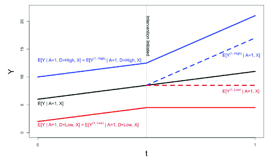
Figure 1: An example of Assumption 4 where exposure level is discretized into high and low dose for visualization.

While assumptions regarding parallel trends are by definition untestable using observed data, it is common for practitioners to test for counterfactual parallel trends between the treated and control groups leading up to the intervention when multiple pre-treatment observations are available (e.g., $t=-1$) under a binary treatment.(Bilinski and Hatfield, 2018) The test derives its usefulness by assuming the fully observable relationship between $E[Y_{0}^{(0,\emptyset)}-Y_{-1}^{(0,\emptyset)}|A=1]$ and $E[Y_{0}^{(0,\emptyset)}-Y_{-1}^{(0,\emptyset)}|A=0]$ is a reasonable proxy for the unobservable relationship between $E[Y_{1}^{(0,\emptyset)}-Y_{0}^{(0,\emptyset)}|A=1]$ and $E[Y_{1}^{(0,\emptyset)}-Y_{0}^{(0,\emptyset)}|A=0]$. Similar placebo tests are possible for Assumption 4, however part of this assumption, $E[Y_{t}^{(1,\delta)}|A=1]$, is unobservable even in the pre-treatment period. Therefore, the usefulness of comparable tests assessing $E[Y_{0}^{(0,\emptyset)}-Y_{-1}^{(0,\emptyset)}|A=1,D=\delta]=E[Y_{0}^{(0,\emptyset)}-Y_{-1}^{(0,\emptyset)}|A=1]$ also depends on how well these trends represent counterfactual trends at different exposure levels.

The final two assumptions are extensions of standard causal inference assumptions to the continuous exposure setting:

Assumption 5 (Consistency)

$Y_{it}^{(z_{it},d_{it})}=Y_{it}$ when $(Z_{it},D_{it})=(z_{it},d_{it})$

Assumption 6 (Positivity)

There is $\epsilon>0$ such that

(i) $\epsilon\leq\pi_{A}(\mathbf{x})<1$ for all $\mathbf{x}\in\mathbbm{X}$ and

(ii) $\epsilon\leq\pi_{D}(\delta|\mathbf{x},A=1)$ for all $\mathbf{x}\in\mathbbm{X}|A=1,\text{ }\delta\in\mathbbm{D}$,

where $\pi_{A}(\mathbf{x})=P(A=1|\mathbf{x})$ and $\pi_{D}(\delta|\mathbf{x},A=1)=f(\delta|A=1,\mathbf{X})$.

Here, we require a stricter positivity assumption (Assumption 6) than the binary setting, which only requires Assumption 6(i). Assumption 6(ii) relates to covariate overlap between the different dose levels and would violated if certain subpopulations, defined by confounders $\mathbf{X}$, were restricted from certain exposure levels.

After these assumptions, we then can frame (1) and (2) fully with observable data as:

Theorem 1 (Identifiability)

Under Assumptions 1-6, (1) is identifiable through $\Psi(\delta)=E[\mu_{1,\Delta}(\delta,\mathbf{X})-\mu_{0,\Delta}(\mathbf{X})|A=1]$, where $\mu_{1,\Delta}(\delta,\mathbf{X})=E[Y_{1}-Y_{0}|A=1,D=\delta,\mathbf{X}]$ and $\mu_{0,\Delta}(\mathbf{X})=E[Y_{1}-Y_{0}|A=0,\mathbf{X}]$.

Accordingly, (2) is then identifiable through $\Psi=E[\Psi(D)|A=1]$.

2.3 Multiply-Robust Estimator

An ideal estimator for (1) would then be based on the efficient influence function (EIF) for this estimand, as EIF-based estimators come with optimal convergence properties and often, though not necessarily, certain robustness to model misspecification. However, the EIF is not tractable for (1) without requiring parametric restrictions on the form of the otherwise infinite-dimensional curve as such a curve does not satisfy the requirement for pathwise differentiability.(Kennedy, 2022) Parametric restrictions generally limit method applicability and data fit, so we do not consider this a viable path forward. However, the EIF for (2) is tractable and given by:

Theorem 2 (Efficient Influence Function for $\Psi$)

The efficient influence function for $\Psi$, is given by:

$$\phi(\mathbf{O})=\frac{A}{P(A=1)}\xi(Y_{1},Y_{0},A,D,\mathbf{X})+\tau(Y_{1},Y_{0},A,\mathbf{X})+J(A,\mathbf{X})-\Psi$$

Where

$$\xi(Y_{1},Y_{0},A,D,\mathbf{X}) =m(D)+\frac{(Y_{1}-Y_{0})-\mu_{1,\Delta}(D,\mathbf{X})}{\pi_{D}(D|A=1,\mathbf{X})}f(D|A=1)$$

$$\tau(Y_{1},Y_{0},A,\mathbf{X}) =\frac{A}{P(A=1)}\mu_{0,\Delta}(\mathbf{X})+\frac{1-A}{P(A=1)}\frac{\pi_{A}(\mathbf{X})}{1-\pi_{A}(\mathbf{X})}[(Y_{1}-Y_{0})-\mu_{0,\Delta}(\mathbf{X})]$$

$$J(A,\mathbf{X}) =\frac{A}{P(A=1)}[\int\limits_{\mathbbm{D}}\{\mu_{1,\Delta}(d,\mathbf{X})-m(d)\}df(d|A=1)]$$

And $m(D)=\int\limits_{\mathbbm{X}}\mu_{1,\Delta}(D,\mathbf{x})dP(\mathbf{x}|A=1)$, $f(D|A=1)=\int\limits_{\mathbbm{X}}\pi_{D}(D|A=1,\mathbf{x}))dP(\mathbf{x}|A=1)$

While notationally complex, the resulting influence function is largely intuitive. Note that $\xi(\mathbf{Y_{1},Y_{0},A,D,\mathbf{X}})$ strongly corresponds to $E[Y_{1}-Y_{0}|A=1,D=D]=E[Y_{1}(1,D)-Y_{0}(0,\emptyset)|A=1]$. Here, $m(D)$ averages the conditional expectation, $\mu_{1,\Delta}(D,\mathbf{X})=E[Y_{1}-Y_{0}|A=1,D,\mathbf{X}]$ across all covariates in the treated group. The second term of $\xi$ re-weights observed deviations from expectation by the balance-inducing generalized propensity score weight, $w^{(1)}=f(D)/\pi_{D}(D|A=1,\mathbf{X})$, as a sort of bias correction term when $\mu_{1,\Delta}$ is misspecified. Similarly, $\tau(Y_{1},Y_{0},A,\mathbf{X})$ correseponds to $E[Y_{1}-Y_{0}|A=1]=E[Y_{1}(0,\emptyset)-Y_{0}(0,\emptyset)|A=1]$, where now we plug in treated unit covariates to $\mu_{0,\Delta}(\mathbf{X})=E[Y_{1}-Y_{0}|A=0,\mathbf{X}]$. The second term re-weights observed deviations from expectation for the control group by ATT propensity score weights, $w^{(0)}=\pi_{A}(\mathbf{X})/(1-\pi_{A}(\mathbf{X}))$ as a sort of bias correction term when $\mu_{0}$ is misspecified. Finally, we note that $J(\mathbf{A,\mathbf{X}})$ is independent of exposure dose and $E[J(\mathbf{A,\mathbf{X}})|A=1]=0$, so will not factor into point estimation for either (1) or (2). A similar decomposition for $\xi$ and $J$ was noted by Kennedy et al. (2017) to generate their so-called pseudo-outcomes when estimating a dose response curve for $E[Y^{(\delta)}]$ under a cross-sectional study design.

Utilizing this influence function and subsequent decomposition, we then can estimate (1) and (2) with an multi-step, plug-in procedure:

1. Estimate nuisance functions as $\hat{\pi}_{D},\hat{\pi}_{A},\hat{\mu}_{1,\Delta},\hat{\mu}_{0,\Delta}$.

2. Plug in data and estimated nuisance functions to construct $\hat{\tau}(\mathbf{O};\hat{\pi}_{A},\hat{\mu}_{0,\Delta})$ and take the empirical mean of $\hat{\tau}$ to obtain $\hat{\theta}_{0}$.

3. Plug in data and estimated nuisance functions to construct $\hat{\xi}(\mathbf{O};\hat{\pi}_{D},\hat{\mu}_{1,\Delta})$ and regress $\hat{\xi}$ on dose variable $D$ using a flexible regression function $r_{n}(\hat{\xi},D)$ to obtain $\hat{\theta}(\delta)$.

4. For (1), take the difference $\hat{\theta}(\delta)-\hat{\theta}_{0}$ as $\hat{\Psi}(\delta)$.

5. For (2), take the empirical mean of $\frac{A}{P(A=1)}\hat{\xi}-\hat{\tau}$ as $\hat{\Psi}$.

Practically speaking, $\hat{\pi}_{D}$ and $\hat{\mu}_{1,\Delta}$ must be estimated only using data from the $A=1$ group whereas $\hat{\pi}_{A}$ requires data from both $A=1$ and $A=0$ groups. Estimation of $\hat{\mu}_{0,\Delta}$ could incorporate data from both $A=1$ and $A=0$ groups, but the efficiency gained from utilizing $A=1$ data comes at the cost of robustness in that correctly specifying $\hat{\mu}_{0,\Delta}$ would require properly modeling treatment effect dynamics, linking its specification to that of $\hat{\mu}_{1,\Delta}$. Another generally beneficial step in practice is to normalize $w^{(1)}$ and $w^{(0)}$ to both have mean one as in Hajek weighted estimators, which has previously been noted as important for improving the stability of doubly robust DiD estimators.(Sant’Anna and Zhao, 2020)

The decomposition of the influence function $\phi$ also suggests components related to doubly-robust estimators for both $E[Y_{1}(1,D)-Y_{0}(0,\emptyset)|A=1]$ and $E[Y_{1}(0,\emptyset)-Y_{0}(0,\emptyset)|A=1]$, foreshadowing the multiple robustness properties of our proposed estimator:

Theorem 3 (Multiple Robustness)

Suppose that Assumptions 1-6 hold. Additionally assume that:

1. At least one of the dose-specific nuisance functions {$\pi_{D}$, $\mu_{1,\Delta}$} are correctly specified.

2. At least one of the intervention-specific nuisance functions {$\pi_{A}$, $\mu_{0,\Delta}$} are correctly specified.

Then, $\hat{\Psi}$ is a consistent estimator for (2). Further, if $r_{n}(\xi,d)$ is a regression estimator such that $r_{n}(\xi,d)\overset{p}{\to}E[\xi|D=d]$, then $\hat{\Psi}(\delta)$ is a consistent estimator for (1) when $\delta$ is an exposure value in the interior of the compact support of $D$.

Thereby, we only require one correct model specification in each specified pair of nuisance functions corresponding to $E[Y_{1}(1,D)-Y_{0}(0,\emptyset)|A=1]$ and $E[Y_{1}(0,\emptyset)-Y_{0}(0,\emptyset)|A=1]$, respectively. Accordingly, our estimator will result in consistent effect estimation in 9 of the 16 ($56\%$) permutations of correct/incorrect nuisance function specifications (i.e., {$\pi_{D}\in\{\text{Correct,Incorrect}\},\mu_{1,\Delta}\in\{\text{Correct,Incorrect}\},\pi_{A}\in\{\text{Correct,Incorrect}\},\mu_{0,\Delta}\in\{\text{Correct,Incorrect}\}$}). Compared to standard doubly robust estimators which only require two nuisance functions and thus achieve consistent effect estimation in 3 of the 4 ($75\%$) specification permutations, we see the required cost of addressing multiple levels of confounding in terms of robustness. However, if we consider the specification of both outcome models, $\{\mu_{1,\Delta},\mu_{0,\Delta}\}$, together and both propensity score models, $\{\pi_{D},\pi_{A}\}$, together, then we have consistent estimates in 3 of the 4 specification permutations and further achieve consistency under additional “partial” misspecifications.

The requirements regarding $r_{n}$ suggest the use of a flexible non-parametric regression function to avoid misspecifying the conditional density of $\xi$ given $D$. Following Kennedy et al. (2017), we specifically consider a local linear kernel regression estimator for $r_{n}$, which is a non-parametric estimator imposing relatively few regularity conditions regarding effect curves and nuisance functions for consistency in this framework (Appendix).

2.4 Uncertainty Quantification

Calculating confidence intervals for these multi-step estimators is non-trivial, particularly for $\Psi(D)$ which does not absorb the semi-parametric efficiency guarantees of influence-function based estimators for binary treatments when all nuisance functions are well-specified. Since standard non-parametric regressors are consistent but centered at a smoothed version of the effect curve, rather than the true curve, we adapt previous works in expressing uncertainty about this smoothed curve (Wasserman, 2006; Kennedy et al., 2017). While our estimator is asymptotically normal under mild restrictions on nuisance function convergence rates (Appendix), we note that such results ignore finite-sample uncertainty in the estimation of nuisance functions and may lead to underestimated variances (Lunceford and Davidian, 2004). Thereby, we consider two alternative approaches.

First, we follow previous approaches that represent plug-in causal inference estimators as a series of unbiased estimating equations (i.e., score equations for specified parametric nuisance function models, sample mean equation for $\theta_{0}$ using $\hat{\tau}_{i}$, and kernel regression equation for $\hat{\theta}(D)$ using $\hat{\xi}_{i}$) and apply M-estimation theory to engineer sandwich estimators for the variance of estimated parameters.(Stefanski and Boos, 2002; Cole et al., 2023) Concretely, this approach first defines the estimating equation $\Gamma_{i}(\eta,\delta)$ by:

$$\sum\limits_{i=1}^{n}\Gamma_{i}(\eta,\delta)=\sum\limits_{i=1}^{n}\begin{bmatrix}\theta(\delta)-\ell_{i}(\delta)\hat{\xi_{i}}\\ \theta_{0}-\hat{\tau_{i}}\\ A_{i}S_{\pi_{D}}(Y_{i1},Y_{i0},D_{i},\mathbf{X}_{i};\alpha^{(D)},\sigma^{2})\\ A_{i}S_{\mu_{1}}(Y_{i1},Y_{i0},D_{i},\mathbf{X}_{i};\beta^{(D)})\\ S_{\pi_{A}}(Y_{i1},Y_{i0},\mathbf{X}_{i};\alpha^{(A)})\\ (1-A_{i})S_{\mu_{0}}(Y_{i1},Y_{i0},\mathbf{X}_{i};\beta^{(0)})\end{bmatrix}=0$$

where $\eta=(\theta(\delta),\tau,\alpha^{(D)},\sigma^{2},\beta^{(D)},\alpha^{(A)},\beta^{(0)})$ are estimable parameters; $S_{\pi_{D}}$, $S_{\mu_{1}}$, $S_{\pi_{A}}$, and $S_{\mu_{0}}$ are score equations for parametric nuisance models; and $\ell_{i}(\delta)$ are the local linear kernel regression estimation weights.(Wasserman, 2006) We then use the sandwich variance formula as:

$$\hat{V}(\hat{\eta})=\{\sum\limits_{i=1}^{n}\frac{\partial}{\partial\eta^{\prime}}\Gamma_{i}(\hat{\eta})\}^{-1}\{\sum\limits_{i=1}^{n}\Gamma_{i}^{\bigotimes 2}(\hat{\eta})\{\sum\limits_{i=1}^{n}\frac{\partial}{\partial\eta}\Gamma_{i}^{\prime}(\hat{\eta})\}^{-1}$$

Finally, we can calculate $\hat{V}(\hat{\Psi}(\delta))=V(\hat{\theta}(\delta)-\hat{\theta}_{0})=\hat{V}_{1,1}(\hat{\eta})+\hat{V}_{2,2}(\hat{\eta})-2\hat{V}_{1,2}(\hat{\eta})$ and derive $95\%$ confidence intervals under a normal approximation for each $\delta$. The calculated sandwich estimator under linear ($\pi_{D},\mu_{1,\Delta},\mu_{0,\Delta}$) and logistic ($\pi_{A}$) models is provided in the Appendix.

Still, this sandwich estimator only applies for a restricted set of nuisance function models, which may be inadequate for complex dynamics, and rely on correct specification of all nuisance functions. Alternatively, bootstrapping approaches can be used to express pointwise uncertainty about the smoothed kernel estimate under certain regularity conditions like those required for consistency of $r_{n}$ described in the Appendix.(Wasserman, 2006) Further, bootstrap approaches have been shown to better account for finite sample variability and model misspecification than parametric formulations of asymptotic approximations for previous doubly robust estimators.(Funk et al., 2011) Throughout this paper, we implement a non-parametric weighted bootstrap where we sample unit-specific, rather than observation-specific, weights to account for correlation between multiple observations of the same unit. After sampling these weights from an $exponential(1)$ distribution, we then scale the weights such that the sum of weights in each treatment group are equal to their observed sample sizes and utilize these weights for each fitted model and population mean required in the estimation process. Allowing for small but non-zero weights, unlike a discrete bootstrap sampling approach, is particularly helpful for stabilizing bootstrap sample estimates which otherwise may only have data from a few exposure levels. We then estimate the $2.5$ and $97.5$ percentiles among 500 bootstrap replicates as our interval bounds.

2.5 Multiple Observation Times

For simplicity, we introduced methods with one observation before the intervention ($t=0$) and one observation after ($t=1$). In practice, we often have multiple observation times within these periods that we would like to incorporate additional information from. Following the design of our data example, we consider multiple post-intervention observation times, $m=1,...,M$, where each of these observation times has a corresponding pre-intervention observation time (e.g., corresponding months of the year before and after a policy implementation).(Hettinger et al., 2023) Further, to distinguish from studies involving related to staggered adoption and dynamic treatment regimes, we consider a single intervention time for all treated units where the exposure is constant for all times after the intervention. Presuming our parallel trends assumptions now hold between each of the $m$ pairs of corresponding observation times, we can calculate $m$-time specific effects as defined in the $M=1$ setting and average them over all $m$. Alternative approaches for multiple observation times will depend on the study and we refer the reader to Callaway and Sant’Anna (2021) for frameworks under more complex designs. When estimating outcome-based nuisance functions under multiple observation times, practitioners must consider efficiency and robustness trade-offs when deciding between modeling each observation time separately or incorporating time into a single model. For propensity score models, we utilize a single model to mimic that interventions and exposures are only assigned once, but time-specific weights and their interpretation have been further explored by Stuart et al. (2014). Finally, both mentioned sandwich and bootstrapping uncertainty approaches are readily extensible to this setting. Sandwich estimators require stacking additional estimating equations for each observation time into the formulation of $\Gamma_{i}(\eta,\delta)$, while described bootstrap approaches, which re-sample units, already account for within-unit correlation induced by multiple observations.(Li and Li, 2019)

3 Simulation Studies

We conducted numerical studies to examine the finite-sample properties of our proposed methods relative to alternative approaches under different forms of model misspecification. Specifically, our data generating mechanism, which roughly matches the structure of our data example in the following section, simulated normally distributed covariates,

$$\mathbf{X_{i}}=(X_{i1},X_{i2},X_{i3},X_{i4})^{T}\sim N(\mathbf{0},\mathbf{I}_{4})$$

a binary intervention,

$$A_{i}\mid\mathbf{X_{i}}\sim Bern(expit(-0.3+0.15X_{i1}+0.15X_{i2}-0.15X_{i3}+0.25X_{i4}))$$

$$expit(z)=exp(z)/[1+exp(z)]$$

a normally distributed exposure among treated units,

$$D_{i}\mid\mathbf{X_{i}},A=1\sim N(\mu=6+0.45X_{i1}+0.4X_{i2}-0.45X_{i3}+0.9X_{i4},\sigma^{2}=4)$$

a normally distributed outcome at time $t=0$,

$$Y_{i0}\mid\mathbf{X_{i}},A_{i}\sim N(\mu=10+0.4X_{i1}-X_{i2}+0.4X_{i3}+0.3X_{i4}+2A_{i},\sigma^{2}=0.3^{2})$$

and a normally distributed outcome at time $t=1$ where the expected trend is determined by confounders, intervention group, and exposure level,

$$Y_{i1}\mid\mathbf{X_{i}},A_{i},D_{i}\sim N(\mu=Y_{i0}+A_{i}\lambda_{1}(\mathbf{X_{i}},D_{i})+(1-A_{i})\lambda_{0}(\mathbf{X_{i}}),\sigma^{2}=0.1^{2})$$

$$\lambda_{1}(\mathbf{X_{i}},D_{i})=1+0.2X_{i1}+0.2X_{i2}+0.3X_{i3}-0.1X_{i4}+2A_{i}+$$

$$\hskip 113.81102ptD(0.1-0.1X_{i1}+0.1X_{i3}-0.01/10D^{2})$$

$$\lambda_{0}(\mathbf{X_{i}})=-3-X_{i1}+0.7X_{i2}+0.6X_{i3}-0.6X_{i4}$$

To analyze the simulated data, we compared our proposed, multiply robust method (MR) to four alternative estimators. First, we estimated a standard linear two-way fixed effects (TWFE) model, $Y_{it}=\beta_{0}+\boldsymbol{\beta}^{\prime}\mathbf{X_{i}}+\gamma_{T}t+\gamma_{A}A_{i}+\gamma_{D}A_{i}D_{i}+\tau_{A}tA_{i}+\tau_{D}tA_{i}D_{i}+\epsilon_{it}$, and calculated an effect curve as $\hat{\Psi}^{(twfe)}(\delta)=\hat{\tau}_{A}+\hat{\tau}_{D}\delta$. This is an analogous approach to the model studied by Callaway et al. (2021) that does not adjust for confounding between intervention or exposure levels and outcome trends. Second, we estimated a flexible, confounding-naive difference-in-differences estimator as $\hat{\Psi}^{(naive)}(\delta)=\hat{E}[Y_{1}-Y_{0}|D=\delta,A=1]-\hat{E}[Y_{1}-Y_{0}|A=0]$, where the first expectation is estimated with a local linear kernel regression and the second with a sample mean. Then, we considered outcome regression and IPW analogies to our proposed estimator. The outcome regression approach relies entirely on specification of $\mu_{1,\Delta}$ and $\mu_{0,\Delta}$ and estimates $\hat{\Psi}^{(or)}(\delta)=\hat{E}[\hat{\mu}_{1,\Delta}(\mathbf{X})-\hat{\mu}_{0,\Delta}(\mathbf{X})|A=1]$ with a sample mean over treated units. The IPW approach relies entirely on specification of $\pi_{D}$ and $\pi_{A}$, estimating $\hat{\theta}^{(ipw)}(\delta)=\hat{E}[\hat{w}^{(1)}(Y_{1}-Y_{0})|A=1,D=\delta]$ with a local linear kernel regression and $\hat{\theta}^{(ipw)}_{0}=\hat{E}[\hat{w}^{(0)}(Y_{1}-Y_{0})|A=0]$ with a sample mean over control units, to get $\hat{\Psi}^{(ipw)}(\delta)=\hat{\theta}^{(ipw)}(\delta)-\hat{\theta}^{(ipw)}_{0}$. This is a similar approach to that of Han and Yu (2019) but using the estimated propensity scores for weights rather than covariate adjustment.

We consider nuisance function misspecification by developing models under the specified mean functions, but using $\mathbf{X}$ for covariates in our model under a correct specification and $\mathbf{W}$ for covariates under an incorrect specification, where $\mathbf{W}$ is the same covariate transformation as given in Kang and Schafer (2007). For each of the 16 permuations of nuisance model specification, we then generate 1000 simulated datasets for each of three sample sizes: $n=200$, $1000$, and $10000$. Potential estimators are compared using integrated absolute mean bias and root mean squared error (RMSE) where summations are taken over the density of $D$ as estimated from a super-population with $n=1,000,000$. The $10\%$ of mass at each boundary are excluded from evaluation as these values may not frequently be observed in simulations. Finally, for $n=200$ datasets, we assess finite sample inference properties by calculating the integrated coverage probabilities and interval width of confidence intervals derived from the described sandwich and bootstrap variance approaches for our proposed, multiply robust estimator.

3.1 Results

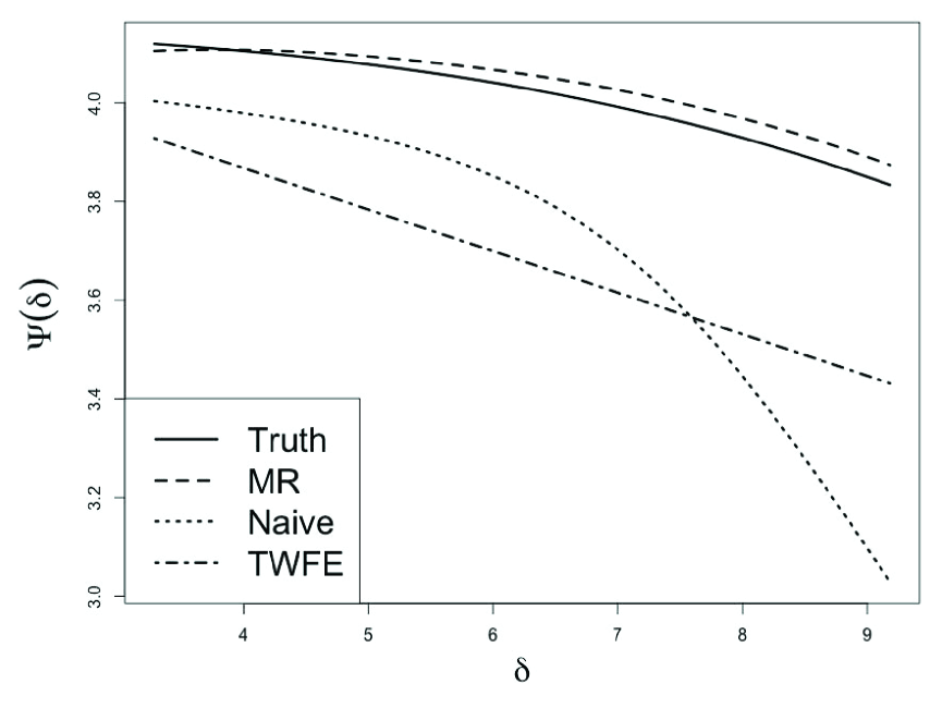
Figure 2: An example fit for one simulated dataset ($n=1000$) showing the true effect curve and estimated effect curves using the multiply robust (MR), confounding-naive (Naive), and two-way fixed effects (TWFE) approaches. A constant difference between the MR and Naive approaches represents confounding between treated and control groups while the increasing difference over values of $\delta$ represents confounding between units at different exposure levels.

Table 1: Comparison of Bias (RMSE) of effect curve estimates under multiply robust (MR), outcome regression (OR), and inverse probability weighting (IPW) approaches in simulation scenarios varying by nuisance function specification ($n=200$). Green cells represent scenarios where both sources of confounding are correctly adjusted for asymptotically, whereas orange and red cells represent scenarios where one and both sources are not correctly adjusted for, respectively. Confounding-naive and two-way fixed effects estimators have Bias (RMSE) of 0.329 (0.169) and 0.384 (0.184) in all scenarios.

Incorrect Models	MR	OR	IPW
None	0.008 (0.019)	0.002 (0.019)	0.015 (0.064)
$\pi_{A}$	0.008 (0.019)	0.002 (0.019)	0.117 (0.09)
$\mu_{0,\Delta}$	0.034 (0.03)	0.089 (0.046)	0.015 (0.064)
$\pi_{D}$	0.008 (0.019)	0.002 (0.019)	0.112 (0.08)
$\mu_{1,\Delta}$	0.028 (0.054)	0.138 (0.056)	0.015 (0.064)
$\pi_{A},\pi_{D}$	0.008 (0.019)	0.002 (0.019)	0.149 (0.112)
$\mu_{0,\Delta},\mu_{1,\Delta}$	0.033 (0.063)	0.186 (0.095)	0.015 (0.064)
$\mu_{0,\Delta},\pi_{D}$	0.034 (0.03)	0.089 (0.046)	0.112 (0.08)
$\pi_{A},\mu_{1,\Delta}$	0.028 (0.054)	0.138 (0.056)	0.117 (0.09)
$\pi_{A},\mu_{0,\Delta}$	0.132 (0.053)	0.089 (0.046)	0.117 (0.09)
$\pi_{D},\mu_{1,\Delta}$	0.119 (0.068)	0.138 (0.056)	0.112 (0.08)
$\pi_{A},\mu_{0,\Delta},\pi_{D}$	0.131 (0.053)	0.089 (0.046)	0.149 (0.112)
$\pi_{A},\mu_{0,\Delta},\mu_{1,\Delta}$	0.140 (0.088)	0.186 (0.095)	0.117 (0.09)
$\pi_{A},\pi_{D},\mu_{1,\Delta}$	0.119 (0.068)	0.138 (0.056)	0.149 (0.112)
$\mu_{0,\Delta},\pi_{D},\mu_{1,\Delta}$	0.116 (0.075)	0.186 (0.095)	0.112 (0.08)
$\pi_{A},\mu_{0,\Delta},\pi_{D},\mu_{1,\Delta}$	0.179 (0.11)	0.186 (0.095)	0.149 (0.112)

Table 2: A comparison of Coverage Probabilities (Interval Widths) for confidence intervals derived from sandwich and bootstrap variances for the proposed, multiply robust estimator in simulation scenarios varying by nuisance function specification ($n=200$).

Incorrect Models	Sandwich	Bootstrap
None	99.1 (0.77)	94.4 (0.52)
$\pi_{A},\pi_{D}$	99.0 (0.77)	94.5 (0.52)
$\mu_{0,\Delta},\mu_{1,\Delta}$	96.2 (0.93)	94.3 (0.85)
$\pi_{A},\mu_{0,\Delta},\pi_{D},\mu_{1,\Delta}$	85.2 (0.90)	84.4 (0.87)

Results summarizing the performance of causal effect curve point estimates are given in Table 1. In all analyzed scenarios, $\hat{\Psi}^{(twfe)}(\delta)$ and $\hat{\Psi}^{(naive)}(\delta)$ exhibit significant bias as they fail to account for confounding between the treated and control groups and between the different exposure levels within the treated group. When $\hat{\pi}_{A}$ or $\hat{\pi}_{D}$ are misspecified ($75\%$ of scenarios), $\hat{\Psi}^{(ipw)}(\delta)$ demonstrates bias, the severity of which depends upon the specific models that are misspecified. Similarly, $\hat{\Psi}^{(or)}(\delta)$ is biased whenever $\hat{\mu}_{0,\Delta}$ or $\hat{\mu}_{1,\Delta}$ are misspecified ($75\%$ of scenarios). On the contrary, our proposed estimator, $\hat{\Psi}^{(mr)}(\delta)$, exhibits bias only when both $\hat{\pi}_{A}$ and $\hat{\mu}_{0,\Delta}$ or both $\hat{\pi}_{D}$ and $\hat{\mu}_{1,\Delta}$ are misspecified ($44\%$ of scenarios). Further, $\hat{\Psi}^{(mr)}(\delta)$ correctly accounts for at least one of the two sources of confounding as long as one of the four nuisance functions are well-specified.

Under correct nuisance function specification, $\hat{\Psi}^{(mr)}(\delta)$ and $\hat{\Psi}^{(or)}(\delta)$ demonstrate the lowest RMSE and thus most efficient estimates. The RMSE of $\hat{\Psi}^{(ipw)}(\delta)$, roughly 5x that of $\hat{\Psi}^{(mr)}(\delta)$ and $\hat{\Psi}^{(or)}(\delta)$ in well-specified scenarios, demonstrates the instability of approaches that rely solely on weighting even under correct model specification. Still, $\hat{\Psi}^{(mr)}(\delta)$ performance may be subject to similar instability when outcome models are misspecified.

Bootstrapped confidence intervals for $\hat{\Psi}^{(mr)}$ generally achieve the specified coverage probabilities in scenarios with consistent effect estimates, suggesting multiply robust inference in these simulations. Robustness of inference has not been proven theoretically for bootstrap approaches but has been observed frequently in practice (Funk et al., 2011). The sandwich variance estimator is conservative under correct nuisance function specification, likely due to the sample size considered ($n=200$) and the asymptotic reliance of similar approaches noted previously (Lunceford and Davidian, 2004). Additionally, the sandwich variance estimator is not robust to any nuisance function misspecification due to its fully parametric specification and only achieves the specified coverage bounds when all models are correctly specified.

4 Application to Nutritional Excise Taxes

4.1 Philadelphia Beverage Tax Study

We applied the proposed methodology to estimate the effects of an excise tax on sugary and sweetened beverages implemented in January 2017 in Philadelphia, Pennsylvania. Previous studies have largely used difference-in-differences methods to estimate the average effect of the tax on volume sales of taxed beverages in Philadelphia and non-taxed neighboring county stores (Roberto et al., 2019; Hettinger et al., 2023; Cawley et al., 2019). Although these studies assessed the impact of the tax as a binary intervention, they identified two significant mechanisms contributing to heterogeneous exposure to the policy. First, as the tax was imposed on the distributor, each individual store had the discretion to determine the extent of corresponding price adjustments. While prior commentaries have speculated that consumers might be more responsive to the awareness of the tax than actual price fluctuations, this hypothesis has yet to be rigorously investigated. Second, compelling evidence suggests a pattern of cross-border shopping in that neighboring non-taxed counties demonstrated a concurrent increase in sales during the tax implementation period. Prior studies have established associations between distance to the border and magnitude of tax effects, but lacked a robust causal framework to effectively control for confounding factors between border proximity and beverage sales (Cawley et al., 2019; Hettinger et al., 2023). A comprehensive understanding of the heterogeneity in tax effects related to both of these exposures is crucial for informing the design of future policies.

In the analysis, we considered 140 pharmacies from Philadelphia as our treated group and 123 pharmacies from Baltimore and non-neighboring Pennsylvania counties as our control group. Data provided by Information Resources Inc. (IRI) and described previously includes volume sales of taxed beverages aggregated in each 4-week period in the year prior to (2016) and after (2017) tax implementation ($m=1,...,13$) (Muth et al., 2016; Roberto et al., 2019). To account for variations in store size, we scaled volume sales for each store by their average 4-week sales in 2016. This scaling not only mitigates many differences in outcome trends between stores in our study, but also facilitates attempts to generalize effects to regions where stores may have a different magnitude of beverage sales.

To quantify the first source of exposure heterogeneity, we assessed the weighted price of taxed beverages per ounce. The measure for price change was determined by calculating the difference between the average metric in the first 4-week period of 2017 (post-tax price) and the average metric across all of 2016 (pre-tax price). Here, we excluded prices after January 2017 from our calculation as these may be influenced by post-tax sales and could incorrectly associate our exposure measure with effect heterogeneity. For the second source of exposure heterogeneity, we calculated, for each store, the percentage of adjacent zip codes also subject to the tax as a measure of protection from cross-border shopping. Unfortunately, the de-identification of stores in our data besides zip code prevented the calculation of a more detailed distance or protection metric. When evaluating effects according to each exposure, we considered several confounding variables including the alternative exposure measure (for models on the treated group), the pre-tax price and sales at a given store, and both the percentage of white residents and average income per household in the zip-code.

We used the proposed kernel smoothing approach to estimate the full effect curve flexibly and estimated our nuisance functions using SuperLearner to limit the potential for model misspecification (van der Laan et al., 2007). Specifically, we included a comprehensive ensemble of generalized linear models, generalized additive models, Lasso, and boosting algorithms as candidate learners for the conditional mean functions of our binomial ($\hat{\pi}_{A}$) and gaussian ($\hat{\pi}_{D},\hat{\mu}_{0,\Delta},\hat{\mu}_{1,\Delta}$) exposures and outcomes. To model the conditional density function of the continuous exposure, we followed previous methodologies to model the squared residuals from the mean model, $\hat{\epsilon}_{i}^{2}$, using SuperLearner under the same set of learners and then estimate the density of $(D_{i}-\hat{D}_{i})/\sqrt{\hat{\epsilon}_{i}^{2}}$ (Hirano and Imbens, 2004; Kreif et al., 2015). To account for the point mass at $D=100\%$ in the second exposure, we estimated the density at this point separately by treating the point as a binomial dependent variable.

4.2 Analysis of Effect Curves

Our exposure measures exhibited substantial heterogeneity. $10\%$ of Philadelphia stores actually decreased their price of taxed beverages following the tax, whereas $59\%$ increased their price by more than the tax amount ($\$0.015$/oz.). $40\%$ of Philadelphia stores were $100\%$ surrounded by other Philadelphia zip codes and the IQR of the remaining $60\%$ of stores was $55-92\%$ surrounded. All confounding variables were significantly associated with the intervention, exposure, and outcome trends in generalized linear models where all confounding variables were included in an additive fashion.

We first used our methodology to assess for parallel trends in the pre-treatment period as described in a previous section by testing known placebo effects for the trends between $m=1$ and $m=2,...,13$ in 2016. In spirit, we treat January 2016 as the “pre-intervention”, $t=0$, time period and the subsequent 2016 periods individually as “post-intervention”, $t=1$, time periods. In addition to only serving as a proxy for the untestable counterfactual parallel trends assumptions, these placebo tests do not directly assess conditional parallel trends in the pre-treatment period as such tests would require estimation of particular parameters in parametric models (limiting confounder adjustment) or conditional effects by $\mathbf{X}$ (an active and challenging area of research in its own right). Instead, these placebo tests assess whether any confounding exists on the population level after adjusting for potential confounders using our methodology. Previous work has used this approach to assess conditional parallel trends in the binary setting (Hettinger et al., 2023). In our setting, our methods generally estimated placebo effects with magnitudes between $10-30\%$ those of non-placebo effects presented in the subsequent section, suggesting observed deviations from parallel trends would explain only a portion of our estimated effects. The only trend exhibiting high risk for violations of parallel trends in the pre-treatment period came between periods $m=1$ and $m=13$, which may indicate consumers adjusting shopping behavior prior to the tax, a violation of Assumption 1 rather than Assumption 4.

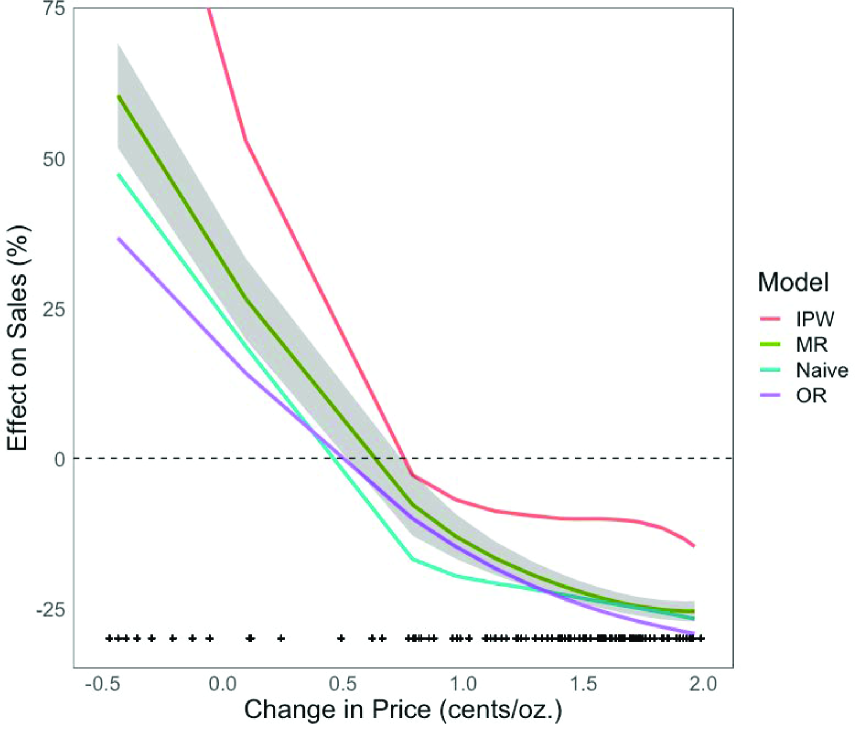
Figure 3: Causal effect curve estimates representing the effect of the tax where all Philadelphia stores change their price by $x$ cents per ounce. Estimates are calculated using the multiply robust (MR), inverse probability weighted (IPW), outcome regression (OR), and confounder-naive (Naive) approaches with pointwise confidence intervals derived for the multiply robust estimator from bootstrapped variance estimates (shaded).

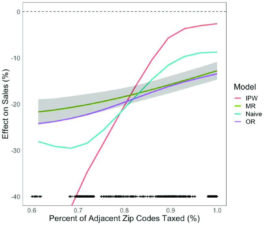
Figure 4: Causal effect curve estimates representing the effect of the tax where all Philadelphia stores are $x\%$ surrounded by taxed zip codes. Estimates are calculated using the multiply robust (MR), inverse probability weighted (IPW), outcome regression (OR), and confounder-naive (Naive) approaches with pointwise confidence intervals derived for the multiply robust estimator from bootstrapped variance estimates (shaded).

Effect curves for both exposure measures under the described multiply robust, IPW, outcome regression, and confounder-naive approaches are visualized with bootstrapped confidence intervals for the multiply robust estimator in Figures 3 and 4. When assessing effect curves related to specific price changes, we saw strong evidence that consumers are responding to specific price changes even after adjusting for observed confounders, regardless of estimator. If all stores were to actually decrease their price following the tax, we estimated that the tax would actually increase sales, whereas if all stores increased their price by $\$0.02$/oz., we estimated that the tax would decrease sales by about $25\%$. While these estimates demonstrate substantial influences of economic competition, we likely would require incorporation of some sort of economic network to truly interpret such effects under counterfactual scenarios like where all pharmacies had decreased their prices since many of these additional sales come from Philadelphia consumers unlikely to change shopping habits under such a scenario. Still, policymakers could utilize this curve to determine the relative elasticity of consumer shopping habits conditional on the observed alternative price points when designing future policies.

Estimated curves for effects of the tax under different exposures to cross-border shopping may assist policy evaluators in understanding effect heterogeneity resulting from cross-border shopping in Philadelphia. Further, policymakers may use the estimated curve to assess what would have happened had all neighboring counties also been taxed, $\hat{\Psi}^{(dr)}(\delta=100\%)$, compared to if only some had been taxed, e.g., , $\hat{\Psi}^{(dr)}(\delta=80\%)$. This counterfactual scenario was previously explored by Lee et al. (2023), wherein they estimated that the tax would still have had a substantial impact under this implementation. Rather than utilizing a cross-border shopping exposure measure among Philadelphia stores, their analytical approach exploited assumptions about which sale increases in non-taxed neighboring counties would be returned to Philadelphia had neighboring counties also been taxed. In our analysis, we similarly estimated a significant tax effect in this counterfactual scenario, suggesting that the tax would have had a $13\%$ effect on store-level sales had all Philadelphia stores been fully surrounded by taxed zip codes, which falls between the estimated effects ignoring confounding ($9\%$) and the estimated aggregate effect over the observed distribution of doses ($17\%$). Notably, $\hat{\Psi}^{(ipw)}(\delta)$ is quite volatile due to large weights accruing near exposure boundaries, supporting the need for outcome models to improve estimate stability.

5 Discussion

In this paper, we introduced a novel approach for estimating causal effect curves within the framework of difference-in-differences designs. These effect curves enable researchers to explore questions such as, “What would be the average effect of a policy where all units were exposed to the policy at the $\delta$-level?”, while accounting for multiple sources of observed confounding commonly encountered in policy evaluations. Crucially, our approach offers a flexible and multiply robust mechanism for confounder adjustment without requiring any parametric assumptions about the form of the effect curve. Further, our approach can incorporate general machine learning and non-parametric modeling techniques by either imposing a limited set of restrictions or utilizing sample splitting techniques (Bonvini and Kennedy, 2022; Chang, 2020). This flexibility and robustness are particularly vital given the additional modeling complexities in this setting with a continuous exposure and two sources of confounding compared to the standard binary exposure setting. Moreover, by harnessing information from both treatment/exposure and outcome models through an influence function-based estimator, our approach enhances the efficiency of existing approaches that rely solely on the propensity score.

While designed for difference-in-differences studies like the application presented, the fundamental concepts of our approach have broader applications. For example, one can readily extend our methodology to accommodate alternative study designs, such as the controlled interrupted time series, by modifying the presented parallel trends assumptions to the new design and altering the derived influence function according to the newly identified conditional expectations (Lopez Bernal et al., 2018). Further, our specification of potential outcomes under a two-dimensional exposure vector resembles the exposure mapping framework introduced by Aronow and Samii (2017). In this framework, our continuous exposure, $D$, is analogous to their exposure mapping function, $h_{it}(\mathbf{A})$, which represents the amount of exposure received through one’s neighbors. As a result, our approach holds promise for estimation of effects specified under interference, where current approaches are highly sensitive to confounding (Clarke, 2017; Butts, 2021). To fully realize these applications, however, future work will need to address uncertainty estimation under such dependencies between units.

Available Code

Code and an example simulated dataset are provided on GitHub at https://github.com/garyhettinger/DiD-interference.

References

- Pollack Porter et al. [2018] Keshia M. Pollack Porter, Lainie Rutkow, and Emma E. McGinty. The Importance of Policy Change for Addressing Public Health Problems. Public Health Reports, 133(1_suppl):9S–14S, 11 2018. ISSN 0033-3549. doi:10.1177/0033354918788880.
- Chaloupka et al. [2019] Frank J. Chaloupka, Lisa M. Powell, and Kenneth E. Warner. The Use of Excise Taxes to Reduce Tobacco, Alcohol, and Sugary Beverage Consumption. Annual Review of Public Health, 40(1):187–201, 4 2019. ISSN 0163-7525. doi:10.1146/annurev-publhealth-040218-043816.
- Cintron et al. [2022] Dakota W. Cintron, Nancy E. Adler, Laura M. Gottlieb, Erin Hagan, May Lynn Tan, David Vlahov, Madellena Maria Glymour, and Ellicott C. Matthay. Heterogeneous treatment effects in social policy studies: An assessment of contemporary articles in the health and social sciences. Annals of Epidemiology, 70:79–88, 6 2022. ISSN 10472797. doi:10.1016/j.annepidem.2022.04.009.
- Heckman et al. [1997] J. J. Heckman, H. Ichimura, and P. E. Todd. Matching As An Econometric Evaluation Estimator: Evidence from Evaluating a Job Training Programme. The Review of Economic Studies, 64(4):605–654, 10 1997. ISSN 0034-6527. doi:10.2307/2971733.
- Abadie [2005] Alberto Abadie. Semiparametric Difference-in-Differences Estimators. The Review of Economic Studies, 72(1):1–19, 1 2005. ISSN 1467-937X. doi:10.1111/0034-6527.00321.
- Callaway et al. [2021] Brantly Callaway, Andrew Goodman-Bacon, and Pedro H. C. Sant’Anna. Difference-in-Differences with a Continuous Treatment. arXiv, 7 2021.
- Li and Li [2019] Fan Li and Fan Li. Double-Robust Estimation in Difference-in-Differences with an Application to Traffic Safety Evaluation. Observational Studies, 5(1):1–23, 2019. ISSN 2767-3324. doi:10.1353/obs.2019.0009.
- Sant’Anna and Zhao [2020] Pedro H.C. Sant’Anna and Jun Zhao. Doubly robust difference-in-differences estimators. Journal of Econometrics, 219(1):101–122, 11 2020. ISSN 03044076. doi:10.1016/j.jeconom.2020.06.003.
- Han and Yu [2019] Bing Han and Hao Yu. Causal difference-in-differences estimation for evaluating the impact of semi-continuous medical home scores on health care for children. Health Services and Outcomes Research Methodology, 19(1):61–78, 3 2019. ISSN 1387-3741. doi:10.1007/s10742-018-00195-9.
- Hirano and Imbens [2004] Keisuke Hirano and Guido W. Imbens. The Propensity Score with Continuous Treatments. pages 73–84. 7 2004. doi:10.1002/0470090456.ch7.
- Austin [2018] Peter C. Austin. Assessing the performance of the generalized propensity score for estimating the effect of quantitative or continuous exposures on binary outcomes. Statistics in Medicine, 37(11):1874–1894, 5 2018. ISSN 0277-6715. doi:10.1002/sim.7615.
- Díaz and van der Laan [2013] Iván Díaz and Mark J. van der Laan. Targeted Data Adaptive Estimation of the Causal Dose–Response Curve. Journal of Causal Inference, 1(2):171–192, 12 2013. ISSN 2193-3677. doi:10.1515/jci-2012-0005.
- Kennedy et al. [2017] Edward H. Kennedy, Zongming Ma, Matthew D. McHugh, and Dylan S. Small. Non-parametric methods for doubly robust estimation of continuous treatment effects. Journal of the Royal Statistical Society: Series B (Statistical Methodology), 79(4):1229–1245, 9 2017. ISSN 1369-7412. doi:10.1111/rssb.12212.
- Bonvini and Kennedy [2022] Matteo Bonvini and Edward H. Kennedy. Fast convergence rates for dose-response estimation. arXiv, 7 2022.
- Zeldow and Hatfield [2021] Bret Zeldow and Laura A. Hatfield. Confounding and regression adjustment in <scp>difference-in-differences</scp> studies. Health Services Research, 56(5):932–941, 10 2021. ISSN 0017-9124. doi:10.1111/1475-6773.13666.
- de Chaisemartin and D’Haultfoeuille [2022] Clément de Chaisemartin and Xavier D’Haultfoeuille. Two-Way Fixed Effects and Differences-in-Differences with Heterogeneous Treatment Effects: A Survey. Technical report, National Bureau of Economic Research, Cambridge, MA, 1 2022.
- Muñoz and van der Laan [2012] Iván Díaz Muñoz and Mark van der Laan. Population Intervention Causal Effects Based on Stochastic Interventions. Biometrics, 68(2):541–549, 6 2012. ISSN 0006-341X. doi:10.1111/j.1541-0420.2011.01685.x.
- Bilinski and Hatfield [2018] Alyssa Bilinski and Laura A. Hatfield. Nothing to see here? Non-inferiority approaches to parallel trends and other model assumptions. arXiv, 5 2018.
- Kennedy [2022] Edward H. Kennedy. Semiparametric doubly robust targeted double machine learning: a review. arXiv, 3 2022.
- Wasserman [2006] Larry Wasserman. All of Nonparametric Statistics. Springer New York, New York, NY, 2006. ISBN 978-0-387-25145-5. doi:10.1007/0-387-30623-4.
- Lunceford and Davidian [2004] Jared K. Lunceford and Marie Davidian. Stratification and weighting via the propensity score in estimation of causal treatment effects: a comparative study. Statistics in Medicine, 23(19):2937–2960, 10 2004. ISSN 0277-6715. doi:10.1002/sim.1903.
- Stefanski and Boos [2002] Leonard A Stefanski and Dennis D Boos. The Calculus of M-Estimation. The American Statistician, 56(1):29–38, 2 2002.
- Cole et al. [2023] Stephen R Cole, Jessie K Edwards, Alexander Breskin, Samuel Rosin, Paul N Zivich, Bonnie E Shook-Sa, and Michael G Hudgens. Illustration of 2 Fusion Designs and Estimators. American Journal of Epidemiology, 192(3):467–474, 2 2023. ISSN 0002-9262. doi:10.1093/aje/kwac067.
- Funk et al. [2011] Michele Jonsson Funk, Daniel Westreich, Chris Wiesen, Til Stürmer, M. Alan Brookhart, and Marie Davidian. Doubly Robust Estimation of Causal Effects. American Journal of Epidemiology, 173(7):761–767, 4 2011. ISSN 1476-6256. doi:10.1093/aje/kwq439.
- Hettinger et al. [2023] Gary Hettinger, Christina Roberto, Youjin Lee, and Nandita Mitra. Estimation of Policy-Relevant Causal Effects in the Presence of Interference with an Application to the Philadelphia Beverage Tax. arXiv, 1 2023.
- Callaway and Sant’Anna [2021] Brantly Callaway and Pedro H.C. Sant’Anna. Difference-in-Differences with multiple time periods. Journal of Econometrics, 225(2):200–230, 12 2021. ISSN 03044076. doi:10.1016/j.jeconom.2020.12.001.
- Stuart et al. [2014] Elizabeth A. Stuart, Haiden A. Huskamp, Kenneth Duckworth, Jeffrey Simmons, Zirui Song, Michael E. Chernew, and Colleen L. Barry. Using propensity scores in difference-in-differences models to estimate the effects of a policy change. Health Services and Outcomes Research Methodology, 14(4):166–182, 12 2014. ISSN 1387-3741. doi:10.1007/s10742-014-0123-z.
- Kang and Schafer [2007] Joseph D. Y. Kang and Joseph L. Schafer. Demystifying Double Robustness: A Comparison of Alternative Strategies for Estimating a Population Mean from Incomplete Data. Statistical Science, 22(4), 11 2007. ISSN 0883-4237. doi:10.1214/07-STS227.
- Roberto et al. [2019] Christina A. Roberto, Hannah G. Lawman, Michael T. LeVasseur, Nandita Mitra, Ana Peterhans, Bradley Herring, and Sara N. Bleich. Association of a Beverage Tax on Sugar-Sweetened and Artificially Sweetened Beverages With Changes in Beverage Prices and Sales at Chain Retailers in a Large Urban Setting. JAMA, 321(18):1799, 5 2019. ISSN 0098-7484. doi:10.1001/jama.2019.4249.
- Cawley et al. [2019] John Cawley, David Frisvold, Anna Hill, and David Jones. The impact of the Philadelphia beverage tax on purchases and consumption by adults and children. Journal of Health Economics, 67:102225, 9 2019. ISSN 01676296. doi:10.1016/j.jhealeco.2019.102225.
- Muth et al. [2016] MK Muth, M Sweitzer, D Brown, K Capogrossi, S Karns, D Levin, A Okrent, P Siegel, and C Zhen. Understanding IRI household-based and store-based scanner data, 4 2016.
- van der Laan et al. [2007] Mark J. van der Laan, Eric C Polley, and Alan E. Hubbard. Super Learner. Statistical Applications in Genetics and Molecular Biology, 6(1), 1 2007. ISSN 1544-6115. doi:10.2202/1544-6115.1309.
- Kreif et al. [2015] Noémi Kreif, Richard Grieve, Iván Díaz, and David Harrison. Evaluation of the Effect of a Continuous Treatment: A Machine Learning Approach with an Application to Treatment for Traumatic Brain Injury. Health Economics, 24(9):1213–1228, 9 2015. ISSN 1057-9230. doi:10.1002/hec.3189.
- Lee et al. [2023] Youjin Lee, Gary Hettinger, and Nandita Mitra. Policy effect evaluation under counterfactual neighborhood interventions in the presence of spillover. arXiv, 3 2023.
- Chang [2020] Neng-Chieh Chang. Double/debiased machine learning for difference-in-differences models. The Econometrics Journal, 23(2):177–191, 5 2020. ISSN 1368-4221. doi:10.1093/ectj/utaa001.
- Lopez Bernal et al. [2018] James Lopez Bernal, Steven Cummins, and Antonio Gasparrini. The use of controls in interrupted time series studies of public health interventions. International Journal of Epidemiology, 47(6):2082–2093, 12 2018. ISSN 0300-5771. doi:10.1093/ije/dyy135.
- Aronow and Samii [2017] Peter M. Aronow and Cyrus Samii. Estimating average causal effects under general interference, with application to a social network experiment. The Annals of Applied Statistics, 11(4), 12 2017. ISSN 1932-6157. doi:10.1214/16-AOAS1005.
- Clarke [2017] Damian Clarke. Estimating Difference-in-Differences in the Presence of Spillovers. Munich Personal RePEc Archive, 2017.
- Butts [2021] Kyle Butts. Difference-in-Differences Estimation with Spatial Spillovers. arXiv, 5 2021.