A stationary population model with an interior interface-type boundary

Abstract.

We propose a stationary system that might be regarded as a migration model of some population abandoning their original place of abode and becoming part of another population, once they reach the interface boundary. To do so, we show a model where each population follows a logistic equation in their own environment while assuming spatial heterogeneities. Moreover, both populations are coupled through the common boundary, which acts as a permeable membrane on which their flow moves in and out. The main goal we face in this work will be to describe the precise interplay between the stationary solutions with respect to the parameters involved in the problem, in particular the growth rate of the populations and the coupling parameter involved on the boundary where the interchange of flux is taking place.

1. Introduction

In this work we analyse the existence of stationary solutions of two different species living separately in two regions of a heterogeneous environment and having an interaction through a permeable membrane, the common boundary of the two regions.

To be more specific, the problem we have in mind is a reaction-diffusion model with spatially heterogeneous coefficients that provides us with the stationary non-negative solutions for an evolution model of two species, that live separately in two subdomains $\Omega_{1}$ and $\Omega_{2}$ of $\Omega\subset\mathbb{R}^{N}$, see Figure 1 and Section 2 for a precise description of the domain. So that, if we denote the density of these populations by $u_{1},u_{2}$, we have that $u_{i}>0$ in $\Omega_{i}$ and $u_{i}=0$ in $\Omega\setminus\Omega_{i}$, with $i=1,2$. The model that describes their stationary behaviour is shown as

(1.1) $$\left\{\begin{array}[]{llll}-\Delta u_{1}(x)=\lambda m_{1}(x)u_{1}(x)-a_{1}(x)u_{1}(x)^{p},&\quad\text{ in }\Omega_{1},&\\[6.0pt] -\Delta u_{2}(x)=\lambda m_{2}(x)u_{2}(x)-a_{2}(x)u_{2}(x)^{p},&\quad\text{ in }\Omega_{2},&\end{array}\right.$$

where $\lambda$ is a real parameter and $p>1$. The weights $m_{i}$ are assumed to be two positive $L^{\infty}(\Omega_{i})$ functions, so that $\lambda m_{i}(x)$ stands for the intrinsic growth rate of $u_{i}$ respectively. The coefficients $a_{i}(x)$ are two non-negative Hölder continuous functions in $\mathcal{C}^{0,\eta}(\overline{\Omega_{i}})$, for some $\eta\in(0,1]$, that measure the crowding effects of the populations in the corresponding subdomains of $\Omega_{i}$. In order to take into account these effects, we define the following subsets, related to the positivity of the potentials $a_{1}$ and $a_{2}$,

(1.2) $$\Omega_{0}^{a_{1}}:=\{x\in\Omega_{1}\;:\;a_{1}(x)=0\}\quad\text{and}\quad\Omega_{0}^{a_{2}}:=\{x\in\Omega_{2}\;:\;a_{2}(x)=0\}$$

so that $\overline{\Omega}_{0}^{a_{1}}\subset\Omega_{1}$, and $\overline{\Omega}_{0}^{a_{2}}\subset\Omega_{2}$, while $a_{i}$ remain positive in the rest of the subdomain $\Omega_{i}$.

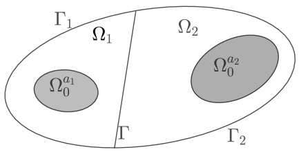
Figure 1. A possible configuration of the domain.

The two populations only interact through the interior boundary, also called interface or membrane $\Gamma$. Moreover, we will consider a hostile outside region. Hence, the boundary conditions read as follows

(1.3) $$\left\{\begin{array}[]{ll}\dfrac{\partial u_{1}}{\partial{\bf n_{1}}}=\dfrac{\partial u_{2}}{\partial{\bf n_{1}}}=\mu(u_{2}-u_{1}),&\quad\text{on }\Gamma,\\[10.0pt] u_{i}=0,&\text{\quad on }\Gamma_{i},\quad\text{with}\quad i=1,2,\\ \end{array}\right.$$

where ${\bf n_{1}}$ is the unitary outward normal vector of $\Gamma$, which points outward with respect to $\Omega_{1}$ and $\mu>0$ is a real parameter, the membrane permeability constant. Note that the intersections between both manifolds $\Gamma_{i}$ and $\Gamma$ satisfy both boundary conditions. Hence, at these points we have the continuity between both sides and the set $\Gamma$ could be assumed to be closed if we include these intersection points, in case of having the standard configuration shown in Figure 1.

The major novelty that we address in this paper stems from the boundary conditions. Indeed, besides the usual Dirichlet data on the boundary of $\Omega$, we also consider an interior interface condition. Our aim is to describe the behaviour of the solutions for that interface problem. The main results that we show, see Sections 5 and 6, state the existence and behaviour of solutions to problem (1.1)–(1.3) considering two different configurations for the potentials $a_{i}$. First, we will deal with the non-degenerate case, in which $a_{i}$ are positive everywhere. We obtain that there exist positive solutions to (1.1)–(1.3) if the parameter $\lambda$ is bigger than a certain $\lambda^{*}$, while below that value $\lambda^{*}$ we just have the trivial solution everywhere. The situation changes radically in the degenerate case, in which we assume two vanishing domains, $\Omega_{0}^{a_{i}}$, inside the subdomains $\Omega_{i}$, where the coefficients $a_{i}$ are neglected. In this case, problem (1.1)–(1.3) has positive solutions if the parameter $\lambda$ is bounded between two precise constants $\lambda^{*}<\lambda<\lambda_{\infty}$. As in the previous case, if $\lambda<\lambda^{*}$ one just finds the trivial solution. If $\lambda\geq\lambda_{\infty}$ we get a blow-up behaviour in uniformly compact subsets of $\Omega_{0}^{a_{i}}$. In the complement of these blow-up regions we find a steady-state solution that blows-up at the border of the regions. We notice that, even though the behaviour we obtain here is similar to a logistic model with spatial heterogeneities and vanishing subdomains (cf. [1]), our model has an important geometrical issue which makes the results more constrained to some conditions. These geometrical aspects give richer situations and allow us to study a novel branch of problems that aim to model situations in which interior membranes appear, a circumstance which has been little studied from a rigorous point of view.

Furthermore, many problems that arise in biology, physics and/or medical science can be modelled by considering two subdomains with a common interior membrane that allows permeation from one domain to the other one. This interface boundary condition, also called the Kedem-Katchalsky interface condition, [21], was introduced in 1961 in a thermodynamic setting. These conditions, describing the flow through the membrane, are compatible with mass conservation lead to flux continuity, and energy dissipation, that gives us that the flux is proportional to the jump of the function through the membrane with proportionality coefficient $\mu$; see [14] for further details.

From a biological point of view, the use of Kedem-Katchalsky interface conditions goes back to [28], where the authors studied the dynamics of the solute in the vessel and in the arterial wall. Since then, biological applications of membrane problems have increased and have been used to describe phenomena such as tumour invasion, transport of molecules through the cell/nucleus membrane, cell polarisation and cell division or genetics, see [14] and references therein.

As far as the study of the mathematical properties is concerned, articles that include a geographical barrier are relatively few. We were only aware of a few works: In [30] a semi-linear parabolic problem is considered. They investigate the effects of the barrier on the global dynamics and on the existence, stability, and profile of spatially non-constant equilibria. A similar problem was previously considered in [12] and [13]. His analysis was mainly in the framework of the existence of weak solutions of parabolic and elliptic differential equations with barrier boundary conditions. The author establishes a new comparison principle, the global existence of solutions, and sufficient conditions of stability and instability of equilibria. He shows, in particular, that the stability of equilibrium changes as the barrier permeability changes through a critical value. Very recently, Ciavolella and Perthame [14] and [15] adapted the well-known $L^{1}$-theory for parabolic reaction-diffusion systems to the membrane boundary conditions case and proved several regularity results. Finally, in [25] a semi-linear elliptic interface problem is studied. The authors analyse the existence and uniqueness of positive solutions, under the assumption that the interface condition in not symmetric, allowing different in and out fluxes of the domain. Although we assume symmetry on the interface our results are also valid for non-symmetric conditions. It is worth mentioning that all these references deal with problems that do not consider refuges (that is $\Omega_{0}^{a_{i}}$ are empty).

Organisation of the paper. — In Section 2 we go through the model we are dealing with and fix the notation that we are going to use throughout the paper. Section 3 is devoted to the study of two auxiliary linear problems that take into account the interface condition. In Section 4 we describe the limit behaviour of a parameter dependent linear elliptic eigenvalue problem that will be crucial to establish the main results of the paper, when applying the method of sub and supersolutions for the existence of solutions. Finally, we state and prove the main results of the paper in Sections 5 and 6. Section 7 is devoted to presenting the conclusions of this paper and to establish some open problems.

2. Preliminaries

The aim of this section is to comment on the special characteristics of the model. In particular, we describe it both from a biological and mathematical point of view. We also describe the notation that we are going to use.

2.1. The model

The equations in (1.1) arise occur in population dynamics as a stationary model of reaction-diffusion equations in which the individuals of a group live in a domain where neither competition or cooperation with other species exists. The model equation

$$-\Delta u(x)=\lambda m(x)u(x)-a(x)u(x)^{p}$$

assuming spatial heterogeneities was first mathematically analysed by Cantrell and Cosner in their seminal paper [11], with $p=2$. Here the population grows following a logistic (when $a>0$) or Malthusian behaviour (in the regions where $a=0$), $\lambda m(x)$ stands for the intrinsic growth rate of the population, since the function $m(x)$ is going to be considered strictly positive, at any point $x$, and $\lambda$ will be a positive parameter. Moreover, $a(x)$ is the so-called intra-specific competition. Therefore, in the regions where $a=0$, the refuges or regions with unlimited resources, the population grows without limits.

Hence, the model we consider here could represent the migration or relation of two groups of the previous population living in different regions of a common habitat, but having some interaction between them, through an interchange of flux on the common boundary, $\Gamma$, that can be seen as a natural or geographical barrier. For the transmission condition

$$\dfrac{\partial u_{1}}{\partial{\bf n_{1}}}=\dfrac{\partial u_{2}}{\partial{\bf n_{1}}}=\mu(u_{2}-u_{1})$$

the parameter $\mu$ measures the strength of the membrane. The flux of individuals remains continuous being proportional to the change of density across the barrier by a rate $1/\mu$. Therefore, the smaller $\mu$ is the stronger the barrier is. And in fact, at the limit, when $\mu\to 0$, there is no transmission across $\Gamma$. The limit problem consists of two populations living separately in two different domains with homogenous mixed boundary conditions, Dirichlet on $\Gamma_{i}$ and Neumann on $\Gamma$, see [9] for properties of this type of problems.

If only one of the populations is zero on $\Gamma$, say $u_{1}$, then, again, the problem for $u_{2}$ becomes uncoupled, with mixed homogenous boundary conditions, Robin on $\Gamma$ and Dirichlet on $\Gamma_{2}$. Clearly, we can understand the problem that defines the behaviour of $u_{1}$ as a problem with non-homogeneous mixed boundary data in $\Omega_{1}$. Moreover, this would also allow the existence of semi-trivial solutions of the type $(u_{1},0)^{T}$ having now $u_{1}$ homogeneous boundary conditions on $\partial\Omega_{1}$.

2.2. Basic notation and functional setting.

Though one of the aims we have in mind consists of understanding this problem as a whole system, in vectorial logistic form in the whole domain $\Omega$, depending on the results and proofs we are dealing with, sometimes it will be more convenient to work with a two equation point of view. For the sake of completeness, we think that it is worth writing this short subsection to state the notation we are going to use throughout the paper.

Domains and geometry: To fix the geometric structure of the problem let $\Omega\subset\mathbb{R}^{N}$, with $N\geq 2$ be a bounded, connected domain. We split $\Omega$ into two non-empty, regular sets, $\Omega_{1}$ and $\Omega_{2}$, such that $\overline{\Omega}=\overline{\Omega}_{1}\cup\overline{\Omega}_{2}$. We will denote by $\Gamma$ the inside boundary, $\Gamma=\overline{\Omega}_{1}\cap\overline{\Omega}_{2}$ and by $\Gamma_{1}:=\partial\Omega_{1}\setminus\Gamma$ and $\Gamma_{2}:=\partial\Omega_{2}\setminus\Gamma$ the outside boundaries. It is worth noting that in Figure 1 we are assuming that $\Gamma_{1}$ and $\Gamma_{2}$ are non-empty. However, it would be also possible to have, say $\Gamma_{1}=\emptyset$ and $\Gamma=\partial\Omega_{1}$ which in turn would mean $\Omega_{1}\subset\Omega_{2}$ (see [27] or [25]). This configuration, though possible and easily applicable, is not considered here. We also assume that these domains, as well as all the possible subsets appearing throughout the paper, are as regular as necessary; let us say with Lipschitz boundary, which again will play a role in obtaining some of the results.

We will use the subscript $1$, respectively $2$, to denote objects (functions, parameters…) defined in $\Omega_{1}$ (resp. $\Omega_{2}$) and each time we write the subscript $i$ we mean $i=1,2$ and we will not mention it anymore.

Vectors: In order to simplify notation, we will use capital letters to denote the vector corresponding to a pair of functions (typically solutions of a system), where the first entry is defined in $\Omega_{1}$, or defined equal to zero in $\Omega_{2}$, and the second one in $\Omega_{2}$. Thus, for example, we will write $U$ to denote the vector $(u_{1},u_{2})^{T}$, where $u_{i}:\Omega_{i}\to\mathbb{R}$ and $U(x)$ will stand for $(u_{1}(x),0)^{T}$ if $x\in\Omega_{1}$ and $(0,u_{2}(x))^{T}$ if $x\in\Omega_{2}$. By abuse of notation we will use $\nabla U$ to denote $(\nabla u_{1},\nabla u_{2})^{T}$. Also, we will write $\Phi>0$ if $\phi_{1}>0$ in $\Omega_{1}$ and $\phi_{2}>0$ in $\Omega_{2}$ and $\Phi\succeq 0$ if we allow one of the components to be identically zero in its domain, while the other one is positive.

Matrices: All the matrices that appear in this paper come from a two equation framework. Hence, they are $2\times 2$ and in most of the cases, diagonal.

We will keep the letter $\mathbf{L}$ to denote the “laplacian diagonal matrix,”  $\mathbf{I}$ will stand for the $2\times 2$ identity matrix and we will denote other matrices using capital boldface letters, for instance

$$\mathbf{L}=\left(\begin{array}[]{cc}-\Delta&0\\ 0&-\Delta\end{array}\right),\qquad\mathbf{F}=\left(\begin{array}[]{cc}f_{1}&0\\ 0&f_{2}\end{array}\right)$$

where $f_{i}$ will be functions. We will denote $\mathbf{L}+\mathbf{F}$ as $\mathbf{L_{F}}$. In Section 5 we will deal with the inverse of the laplacian. With this aim, we will also define the diagonal matrix

(2.1) $${\mathbf{L}^{-1}=\left(\begin{array}[]{cc}(-\Delta)^{-1}&0\\ 0&(-\Delta)^{-1}\end{array}\right)}.$$

As before, we will write $\mathbf{C}>0$ (or $\geq$) to denote a matrix with positive (non-negative) entries and we will write $\mathbf{C}>\mathbf{D}$ if $\mathbf{C}-\mathbf{D}>0$ (respectively $<$ or $\leq$, $\geq$). Moreover, $\mathbf{C}^{+}$ will stand for the positive part of the matrix in the sense that we take the positive part of each entry (which are usually functions) in the matrix.

Integrals: To simplify notation and if no confusion arises, as is commonly occurs in the literature, we will avoid writing differentials on the integrals. It will be understood that integrals in $\Omega$ or $\Omega_{i}$ require $dx$ and integrals over boundaries, for instance $\Gamma$ or $\partial\Omega_{i}$, have a surface differential such as $ds$.

Functional spaces: In order to deal with problem (1.1)–(1.3) and the related ones, described in the next sections, we have to fix our framework. For this reason we denote the space of continuous functions with the flux condition on $\Gamma$ as

$$\mathcal{C}_{\Gamma}(\Omega):=\{\Psi\in\mathcal{C}(\Omega_{1})\times\mathcal{C}(\Omega_{2}):\dfrac{\partial\psi_{1}}{\partial{\bf n_{1}}}=\dfrac{\partial\psi_{2}}{\partial{\bf n_{1}}}=\mu(\psi_{2}-\psi_{1})\ \hbox{on}\ \Gamma\}.$$

As for the continuous functions up to the boundary we will write

$$\mathcal{C}_{\Gamma}(\overline{\Omega}):=\{\Psi\in\mathcal{C}(\overline{\Omega}_{1})\times\mathcal{C}(\overline{\Omega}_{2}):\dfrac{\partial\psi_{1}}{\partial{\bf n_{1}}}=\dfrac{\partial\psi_{2}}{\partial{\bf n_{1}}}=\mu(\psi_{2}-\psi_{1})\ \hbox{on}\ \Gamma\}.$$

We consider, following [27], functions $\psi_{i}$ defined in $\Omega_{i}$ belonging to the spaces $\mathcal{C}_{\star}(\Omega_{i})$ defined as the set of all continuous functions with compact support in $\Omega=\Omega_{1}\cup\Omega_{2}$; that is $\psi_{i}$ is the restriction of a function of compact support in $\Omega$ to the subdomain $\Omega_{i}$ and we define, as before

$$\mathcal{C}_{\star,\Gamma}(\Omega):=\{\Psi\in\mathcal{C}_{\star}(\Omega_{1})\times\mathcal{C}_{\star}(\Omega_{2}):\dfrac{\partial\psi_{1}}{\partial{\bf n_{1}}}=\dfrac{\partial\psi_{2}}{\partial{\bf n_{1}}}=\mu(\psi_{2}-\psi_{1})\ \hbox{on}\ \Gamma\}.$$

Analogously we define the spaces of continuously differentiable and Hölder continuous functions $\mathcal{C}_{\Gamma}^{1}$, $\mathcal{C}_{\Gamma}^{0,\eta}$, $\mathcal{C}_{\Gamma}^{1,\eta}$, $\mathcal{C}^{1}_{\star,\Gamma}$, $\dots$ for some $\eta\in(0,1]$.

We will denote by $\mathcal{L}$ the product space $L^{2}(\Omega_{1})\times L^{2}(\Omega_{2})$, and consider its usual scalar product $\langle\Phi,\Psi\rangle_{\mathcal{L}}=\sum_{i}\langle\varphi_{i},\psi_{i}\rangle_{L^{2}(\Omega_{i})}$ and the induced norm $\|\Phi\|^{2}_{\mathcal{L}}=\langle\Phi,\Phi\rangle_{\mathcal{L}}=\sum_{i}\|\varphi_{i}\|_{L^{2}(\Omega_{i})}^{2}$. Following [14], let $\mathcal{H}_{0}$ be the Hilbert space of functions $H_{0}^{1}(\Omega_{1})\times H_{0}^{1}(\Omega_{2})$, satisfying Dirichlet homogeneous conditions on $\Gamma_{1}$ and $\Gamma_{2}$. Then, we define $\mathcal{H}_{\Gamma}$ as

$$\mathcal{H}_{\Gamma}:=\{\Psi\in\mathcal{H}_{0}:\dfrac{\partial\psi_{1}}{\partial{\bf n_{1}}}=\dfrac{\partial\psi_{2}}{\partial{\bf n_{1}}}=\mu(\psi_{2}-\psi_{1})\ \hbox{on}\ \Gamma\},$$

equipped with the norm

$$\|\Psi\|^{2}_{\mathcal{H}_{\Gamma}}:=\|\nabla\Psi\|^{2}_{\mathcal{L}}=\|\nabla\psi_{1}\|^{2}_{L^{2}(\Omega_{1})}+\|\nabla\psi_{2}\|^{2}_{L^{2}(\Omega_{2})}.$$

Obviously, $\mathcal{H}_{\Gamma}$ is a Hilbert space and we define the scalar product in $\mathcal{H}_{\Gamma}$ as

$$\left\langle\Phi,\Psi\right\rangle_{\mathcal{H}_{\Gamma}}:=\left\langle\nabla\varphi_{1},\nabla\psi_{1}\right\rangle_{L^{2}(\Omega_{1})}+\left\langle\nabla\varphi_{2},\nabla\psi_{2}\right\rangle_{L^{2}(\Omega_{2})}.$$

Thus, since $\mathcal{H}_{\Gamma}$ is a closed linear subspace of $\mathcal{H}_{0}$, it is a Banach space in which the following compact and continuous embedding hold:

(2.2) $$\mathcal{H}_{\Gamma}\hookrightarrow\mathcal{L},\quad{\text{and}\quad\mathcal{H}_{\Gamma}\rightarrow\mathcal{L}_{\Gamma}:=L^{2}(\Gamma)\times L^{2}(\Gamma)}.$$

Moreover, if $\Phi\in\mathcal{H}_{\Gamma}$ we have $\int_{\Gamma}\varphi_{i}^{2}=\int_{\partial\Omega_{i}}\varphi_{i}^{2}$, and due to the trace inequality, we find that

$$\int_{\Gamma}\varphi_{i}^{2}=\|\varphi_{i}\|^{2}_{L^{2}(\partial\Omega_{i})}\leq C_{\Omega_{i}}\|\varphi_{i}\|^{2}_{H^{1}(\Omega_{i})},$$

with $C_{\Omega_{i}}>0$, depending on the domain $\Omega_{i}$. It is worth pointing out that, due to Poincare’s inequality the norms $\|\cdot\|_{\mathcal{H}_{\Gamma}}$ and $\|\cdot\|_{\mathcal{H}_{0}}$ are equivalent. Therefore, if $C_{\Omega}$ is a positive constant, we define a global trace inequality as

$$\left(\int_{\Gamma}\varphi_{1}^{2}+\int_{\Gamma}\varphi_{2}^{2}\right)=\|\Phi\|^{2}_{\mathcal{L}_{\Gamma}}\leq C_{\Omega}\|\Phi\|^{2}_{\mathcal{H}_{\Gamma}}.$$

Finally, we consider the linear operator $\mathbf{L_{F}}:\mathcal{D}(\mathbf{L_{F}})=\mathcal{H}_{\Gamma}\to\mathcal{L}$. Using this framework, we can rephrase our original problem (1.1)–(1.3) as follows:
Find $U\in\mathcal{H}_{\Gamma}$ such that,

(2.3) $$(\mathbf{L}_{-\lambda\mathbf{M}}+\mathbf{A}U^{p-1})U=0,$$

where $U^{p}$ stands for $(u_{1}^{p},u^{p}_{2})^{T}$.

A natural idea of what a positive weak solution is, consists in considering functions that vanish on $\partial\Omega$ but imposing the inside boundary condition. Hence we define a weak solution to (2.3) by formally multiplying (in $\mathcal{L}$) by a test function $\Phi$ and integrating by parts. The precise definition reads as follows:

Definition 2.1.

Let $U\in\mathcal{H}_{\Gamma}$ be positive. We will say that $U$ is a (weak) solution of (2.3) if

$$\int_{\Omega_{1}}\nabla u_{1}\cdot\nabla\varphi_{1}+\int_{\Omega_{2}}\nabla u_{2}\cdot\nabla\varphi_{2}+\int_{\Gamma}\mu(u_{2}-u_{1})(\varphi_{2}-\varphi_{1})=\lambda\langle\mathbf{M}U,\Phi\rangle_{\mathcal{L}}-\langle\mathbf{A}U^{p},\Phi\rangle_{\mathcal{L}},$$

for $\Phi=(\varphi_{1},\varphi_{2})^{T}\in\mathcal{C}_{\star,\Gamma}^{\infty}$.

We define weak sub- and supersolutions as usual; i.e, by replacing in the definition of solution equality by $\leq$ or $\geq$ respectively.

3. Auxiliary problems

This section is devoted to state the general properties for two interface linear problems related to (1.1) that we will use in the next sections. We collect them here for the sake of completeness and refer the reader to [14],  [25], or [30] for the detailed proofs.

3.1. A linear problem

Let us consider the linear problem given by

(3.1) $$\left\{\begin{array}[]{llll}(-\Delta+f_{1}(x))u_{1}(x)=g_{1}(x),&\quad\text{ in }\Omega_{1},&\\[6.0pt] (-\Delta+f_{2}(x))u_{2}(x)=g_{2}(x),&\quad\text{ in }\Omega_{2},&\end{array}\right.\quad$$

together with boundary conditions

(3.2) $$\left\{\begin{array}[]{ll}\dfrac{\partial u_{1}}{\partial{\bf n_{1}}}=\dfrac{\partial u_{2}}{\partial{\bf n_{1}}}=\mu(u_{2}-u_{1}),&\quad\text{on }\Gamma,\\[10.0pt] u_{i}=0,&\text{\quad on }\Gamma_{i},\quad\text{with}\quad i=1,2,\end{array}\right.$$

where $F=(f_{1},f_{2})^{T},G=(g_{1},g_{2})^{T}$ and $F>0$. Using the notation introduced in Section 2 we can rewrite this problem in a more compact form as

(3.3) $$\mathbf{L_{\mathbf{F}}}U={G}\quad\hbox{in}\quad\Omega.$$

Associated with problem (3.1)–(3.2) we define the bilinear form $a:\mathcal{H}_{\Gamma}\to\mathbb{R}$, given by

(3.4) $$a(U,V)=\int_{\Omega_{1}}\nabla u_{1}\cdot\nabla v_{1}+\int_{\Omega_{2}}\nabla u_{2}\cdot\nabla v_{2}+\int_{\Omega_{1}}f_{1}u_{1}v_{1}+\int_{\Omega_{2}}f_{2}u_{2}v_{2}+\int_{\Gamma}\mu(u_{2}-u_{1})(v_{2}-v_{1}),$$

and, consequently, a weak solution of (3.1)–(3.2) is a function $U\in\mathcal{H}_{\Gamma}$ such that

$$a(U,V)=\langle G,V\rangle_{\mathcal{L}}$$

for all $V\in\mathcal{H}_{\Gamma}$.

Theorem 3.1.

If $F\in L^{\infty}(\Omega_{1})\times L^{\infty}(\Omega_{2})$ and $G\in\mathcal{L}$, then (3.1)–(3.2) has a unique weak solution $U$. Moreover, there exits a positive constant $C$, such that

$$\|U\|_{\mathcal{H}_{\Gamma}}\leq C(\|G\|_{\mathcal{L}}+\|U\|_{\mathcal{L}}).$$

Proof.

The proof might be performed after applying Lax-Milgram Theorem by showing first that the biliniear form $a(\cdot,\cdot)$ is continuous and coercive in the Hilbert space $\mathcal{H}_{\Gamma}$. We omit the details here, which can be adapted from [14], [25] and [30]. ∎

Under these conditions, we define the resolvent operator for (3.3), $(\mathbf{L}_{\mathbf{F}})^{-1}\,:\,\mathcal{L}\to\mathcal{H}_{\Gamma}$, by

$$G\in\mathcal{L}\mapsto U:=(\mathbf{L}_{\mathbf{F}})^{-1}G\in\mathcal{H}_{\Gamma},$$

having the following.

Lemma 3.2.

The resolvent operator $(\mathbf{L}_{\mathbf{F}})^{-1}$ is linear, continuous and compact.

Proof.

The continuity and linearity of the resolvent $(\mathbf{L}_{\mathbf{F}})^{-1}$ are clear from Lax-Milgram Theorem. To show the compactness of the resolvent we take a sequence $G_{n}\in\mathcal{L}$ such that

$$\lim_{n\to 0}\|G_{n}-G\|_{\mathcal{L}}=0,$$

and set $U=(\mathbf{L}_{\mathbf{F}})^{-1}G$, $U_{n}=(\mathbf{L}_{\mathbf{F}})^{-1}G_{n}$ for $n\geq 1$. Now, using the bilinear form (3.4), we get

$$a(U_{n}-U,U_{n}-U)=\langle G_{n}-G,U_{n}-U\rangle_{\mathcal{L}},\quad\forall n\geq 1.$$

Since $a(\cdot,\cdot)$ is coercive

$$\|U_{n}-U\|^{2}_{\mathcal{H}_{\Gamma}}\leq C|a(U_{n}-U,U_{n}-U)|=C|\langle G_{n}-G,U_{n}-U\rangle_{\mathcal{L}}|\leq C\|G_{n}-G\|_{\mathcal{L}}\|U_{n}-U\|_{\mathcal{H}_{\Gamma}}.$$

Consequently,

$$\|U_{n}-U\|_{\mathcal{H}_{\Gamma}}\leq C\|G_{n}-G\|_{\mathcal{L}}\to 0,\quad\hbox{as}\quad n\to\infty,$$

showing that the resolvent is a compact operator. ∎

Next, by elliptic regularity, see [24] and [30], and also as a direct consequence of the comparison principle stated in [30], we have the following result:

Theorem 3.3.

Let $F,G\in\mathcal{C}^{0,\eta}(\Omega_{1})\times\mathcal{C}^{0,\eta}(\Omega_{2})$ for some $\eta\in(0,1)$ and $F>0$, then (3.3) has a unique solution $U\in\mathcal{C}^{2,\eta}_{\Gamma}(\Omega)$ that verifies

$$\|U\|_{C^{2,\eta}_{\Gamma}}\leq C\|G\|_{C^{0,\eta}}.$$

Moreover, if $G\geq 0$, then $U\geq 0$.

To end this subsection, let us consider, for $F\in\mathcal{C}^{0,\eta}(\Omega_{1})\times\mathcal{C}^{0,\eta}(\Omega_{2})$ the eigenvalue problem

(3.5) $$\mathbf{L_{\mathbf{F}}}U={\sigma U}\quad\hbox{in}\quad\Omega.$$

This problem will be crucial in the sequel to describe the existence of solutions for the nonlinear problem (2.3). We firs notice that having a compact and positive resolvent, one has that the spectrum of $\mathbf{L_{F}}$ might contain infinitely many isolated eigenvalues (see for instance [8]) and together with the compactness of the operator, we have that the spectrum is discrete and each one of the eigenvalues has finite multiplicity. As it is usual in the literature, see for instance [6], we introduce the following definition.

Definition 3.4.

Given an operator $\mathbf{A}$ and a domain $\mathcal{O}=\mathcal{O}_{1}\cup\mathcal{O}_{2}$, we will say that $\Sigma[\mathbf{A};\mathcal{O}]$ is the principal eigenvalue of $\mathbf{A}$ in $\mathcal{O}$ if $\Sigma[\mathbf{A};\mathcal{O}]$ is the unique value for which $\mathbf{A}\Phi=\Sigma[\mathbf{A};\mathcal{O}]\Phi$ (together with the boundary conditions) possesses a solution $\Phi$ with $\Phi\succeq 0$. Such a function $\Phi$ is called principal eigenfunction.

Note that it is common to assume that the principal eigenfunction is positive in $\mathcal{O}$. In our context we only impose that one of the two components is positive in $\mathcal{O}_{1}$ (or $\mathcal{O}_{2}$), allowing the other one to be identically 0.

Theorem 3.5.

Problem (3.5) has a principal eigenvalue $\Sigma[\mathbf{L_{F}};\Omega]$ which is unique and simple (i.e., the algebraic multiplicity is 1). Moreover, $\Sigma[\mathbf{L_{F}};\Omega]$ is continuous and monotone increasing with respect to $\mu$.

The proof of this result is a consequence of the previous analysis and can be found in [30].

3.2. A weighted linear eigenvalue problem

Let us now extend the results shown for problem (3.5) to a weighted eigenvalue problem of the form

(3.6) $$\mathbf{L_{F}}\Phi=\lambda\mathbf{M}\Phi\quad\hbox{in}\quad\Omega,$$

where $m_{i}$ are assumed to be two positive $L^{\infty}(\Omega_{i})$ functions. Problem (3.6) is the short version of the equivalent problem of finding $(\varphi_{1},\varphi_{2})^{T}\in\mathcal{H}_{\Gamma}$ such that

(3.7) $$\left\{\begin{split}&(-\Delta+f_{1})\varphi_{1}=\lambda m_{1}(x)\varphi_{1}\quad\hbox{in}\quad\Omega_{1},\\ &(-\Delta+f_{2})\varphi_{2}=\lambda m_{2}(x)\varphi_{2}\quad\hbox{in}\quad\Omega_{2}.\end{split}\right.$$

with boundary conditions

(3.8) $${\dfrac{\partial\varphi_{1}}{\partial{\bf n_{1}}}=\dfrac{\partial\varphi_{2}}{\partial{\bf n_{1}}}=\mu(\varphi_{2}-\varphi_{1})\quad\hbox{on}\quad\Gamma,\qquad\varphi_{1}=0\quad\text{on }\Gamma_{1},\qquad\varphi_{2}=0\quad\text{on }\Gamma_{2}.}$$

Similar weighted systems, with the solutions defined in the whole domain $\Omega$, but without the interface boundary condition, were studied in, for instance, [18]. For the one equation setting see [23].

Definition 3.6.

A function $\Psi\in\mathcal{H}$ is said to be strongly positive, denoted by $\Psi\gg 0$, if $\Psi\in\mathcal{C}_{\Gamma}(\Omega)$ and the following two conditions hold:

• For any $x\in\Omega_{i}\cup\Gamma$, $\psi_{i}(x)>0$; and

• for any $y\in\Gamma_{i}$, $\dfrac{\partial\psi_{i}(y)}{\partial\bf n_{i}}<0$ and $\psi_{i}(y)=0$.

Lemma 3.7.

Let $\Phi\in\mathcal{H}_{\Gamma}$ be a non-negative solution of (3.6) associated with a positive eigenvalue $\lambda$. Then $\Phi$ is strongly positive.

Proof.

Let $(\varphi_{1},\varphi_{2})^{T}\in\mathcal{H}_{\Gamma}$ be a non-negative solution of (3.7)–(3.8). Now, following the analysis developed in [26], let $v_{1}\in H_{0}^{1}(\Omega_{1})$ be a positive solution to the auxiliary problem

(3.9) $$\left\{\begin{array}[]{ll}(-\Delta+f_{1})v_{1}=g_{1},&\quad\hbox{in}\quad\Omega_{1},\\ v_{1}=0,&\quad\hbox{on}\quad\partial\Omega_{1},\end{array}\right.\quad\hbox{with}\quad g_{1}=\lambda m_{1}(x)\varphi_{1}\geq 0.$$

By assumption, we have that $\varphi_{1}\geq 0$ on $\Gamma$ and, hence, $\varphi_{1}$ is a supersolution for the auxiliary problem (3.9), such that by the comparison principle and the maximum principle

$$\varphi_{1}\geq v_{1}>0\quad\hbox{in}\quad\Omega_{1}.$$

Furthermore, we show that actually the solution $\varphi_{1}$ is strictly positive on $\Gamma$. Indeed, if we assume that $\varphi_{1}(x_{0})=0$ for some $x_{0}\in\Gamma$, due to Hopf’s Lemma we have that

$$\dfrac{\partial\varphi_{1}(x_{0})}{\partial{\bf n_{1}}}<0,$$

which means that $x_{0}$ is not a minimum of $\varphi_{1}$ in $\overline{\Omega}_{1}$, contradicting the fact that $\varphi_{1}(x_{0})=0$. Therefore, $\varphi_{1}>0$ on $\Gamma$. Condition (ii) is also a direct consequence of Hopf’s Lemma.

On the other hand, we also consider a second auxiliary problem

(3.10) $$\left\{\begin{array}[]{ll}(-\Delta+f_{2})v_{2}=\lambda m_{2}(x)\varphi_{2},&\quad\hbox{in}\quad\Omega_{2},\\ v_{2}=\varphi_{1},&\quad\hbox{on}\quad\partial\Omega_{2}.\end{array}\right.$$

Thanks to the strong maximum principle and since $\varphi_{1}>0$ on $\Gamma\subset\partial\Omega_{2}$ we find that $v_{2}>0$ in $\Omega_{2}$. Consequently, since $\varphi_{2}$ is a supersolution to problem (3.10) it follows that

$$\varphi_{2}\geq v_{2}>0\quad\hbox{in}\quad\Omega_{2},$$

showing the strong positivity of the eigenfunction $\Phi$.

The fact that each $\varphi_{i}\in\mathcal{C}(\Omega_{i})$ follows from elliptic regularity and the previous subsection. ∎

Remark 3.8.

Having that any non-negative solution is actually a strong positive solution is in some sense a way of having the strong Maximum Principle and the existence of a positive strict supersolution. In fact, once we have that the first eigenvalue is positive, by the previous Lemma 3.7 we find that the eigenfunctions associated with it are positive. This provides us with a strict positive supersolution. Indeed, for the operator $\mathbf{L_{F}}+\Lambda{\mathbf{I}}$, with $\Lambda$ a sufficiently large positive constant, positive constants $\Upsilon$ are positive strict supersolutions in the sense that

$$(\mathbf{L}_{\mathbf{F}}+\Lambda{\mathbf{I}})\Upsilon>0\quad\hbox{in}\quad\Omega,\quad\hbox{or}\quad\Upsilon>0\quad\hbox{on}\quad\partial\Omega.$$

Furthermore, we will now prove that the first eigenvalue is actually positive and simple, in the sense of algebraic multiplicity 1, applying Krein-Rutrman Theorem as one of the main ingredients. To do so, the next definition is an important element in order to apply the classical Krein-Rutman Theorem.

Definition 3.9.

Let $P$ be a positive cone with non-empty interior in $\mathcal{H}_{\Gamma}$ and $T:\mathcal{H}_{\Gamma}\to\mathcal{H}_{\Gamma}$ a linear operator. We say that $T$ is strongly positive if

$$T(P\setminus 0)\subset{\rm Int}P.$$

See [5] and [19] for more details on strongly positive operators and positive cones. The next theorem shows that (3.6) has indeed a principal eigenvalue.

Theorem 3.10.

Problem (3.6) has a principal eigenvalue denoted by $\lambda_{1}$. Moreover, $\lambda_{1}$ is real, simple (in the sense of multiplicities) and strictly positive.

The proof of this theorem will relay on the analysis of the eigenvalues of two problems related to (3.6), that we analyse in the following two lemmas.

Lemma 3.11.

Let $r(\mathcal{K}_{\lambda})$ be the spectral radius of the operator $\mathcal{K}_{\lambda}:\mathcal{H}_{\Gamma}\to\mathcal{H}_{\Gamma}$ denoted by

(3.11) $$\mathcal{K}_{\lambda}:=(\mathbf{L}_{\mathbf{F}}+\Lambda\mathbf{I})^{-1}(\lambda\mathbf{M}+(\Lambda+\omega){\mathbf{I}}).$$

For any $\lambda\in\mathbb{R}$ such that

(3.12) $$\lambda m_{i}+(\Lambda+\omega)>0.$$

holds, $r(\mathcal{K}_{\lambda})$ is positive and simple. Moreover, it is the principal eigenvalue of

(3.13) $$\mathcal{K}_{\lambda}\Phi=\sigma\Phi.$$

Proof.

The result is a direct consequence of the Krein-Rutman Theorem (cf. [5, Theorem 3.2]), as well as of several results performed in [17] and [23].

Let us first consider, for a fixed value of $\lambda$, the problem

(3.14) $$\mathbf{L}_{\mathbf{F}-\lambda\mathbf{M}}\Phi=\omega\Phi.$$

It is straightforward to see that $\lambda\in\mathbb{R}$ is an eigenvalue of (3.6) if and only if $\omega=0$ is an eigenvalue of the operator $\mathbf{L}_{\mathbf{F}-\lambda\mathbf{M}}$.

On the other hand, it is also easily seen, see [23] for a weak formulation of the result, that $\omega$ is an eigenvalue of $\eqref{eq:aux.con.omega}$ if and only if $\sigma=1$ is an eigenvalue of problem (3.13), where $\mathcal{K}_{\lambda}$ is an operator denoted by (3.11), for any $\lambda\in\mathbb{R}$. Here $\Lambda$ is a constant (which depends on $\lambda$), chosen sufficiently large, so that condition (3.12) and, thus, $(\mathbf{L}_{\mathbf{F}}+\Lambda\mathbf{I})^{-1}$ exists.

Then, it turns out that $\mathcal{K}_{\lambda}$ is a compact, strongly positive operator (see Definition 3.9). Indeed, first of all observe that thanks to the embedding (2.2), we can ensure that $\mathcal{K}_{\lambda}:\mathcal{H}_{\Gamma}\rightarrow\mathcal{H}_{\Gamma}$ is a compact operator. In order to prove that $\mathcal{K}_{\lambda}$ is strongly positive, let us take $\Phi_{0}\in P\setminus\{0\}$. Thus, thanks to the comparison principle we find that the corresponding components are strictly positive in the interior of the subdomains $\Omega_{i}$ and, thanks to Hopf’s Lemma, we also have that the exterior normal derivatives are negative on the boundary of $\Omega$, where we have homogeneous Dirichlet boundary conditions. In other words, Definition 3.6 is satisfied by $\Phi_{0}$, proving that $\mathcal{K}_{\lambda}$ is strongly positive.

Consequently, due to Krein-Rutman’s Theorem, we have that $\mathcal{K}_{\lambda}$ has positive spectral radius, $r(\mathcal{K}_{\lambda})$, which is a simple eigenvalue of (3.13). Moreover, the associated eigenfunction $\Phi\in{\rm Int}P$ is positive, in the sense that $\Phi\succeq 0$, and there is no other eigenvalue with a positive eigenfunction. Hence, following Definition 3.4, $r(\mathcal{K}_{\lambda})$ is the principal eigenvalue of (3.13). Indeed, thanks to Lemma 3.7 we actually have that the eigenfunction is strongly positive. ∎

Remark 3.12.

It can be seen that, if $\Phi$ is the eigenfunction corresponding to the eigenvalue $\sigma=1$ in problem (3.13), then $\Phi$ is also an eigenfunction for $\omega$ in problem (3.14). The same happens for the pair $(0,\Phi)$ and $(\lambda,\Phi)$ corresponding to (3.14) and (3.6), respectively.

Lemma 3.13.

For any $\omega>0$, there exists $\bar{\lambda}\in\mathbb{R}$ such that $r(\mathcal{K}_{\bar{\lambda}})=1$.

Proof.

First of all observe that, since $(\omega+\Lambda)\mathbf{I}+\lambda\mathbf{M}$ is an increasing function of $\lambda$, we have that, as long as (3.12) holds, $\mathcal{K}_{\lambda_{1}}<\mathcal{K}_{\lambda_{2}}$ for $\lambda_{1}<\lambda_{2}$. Hence, see [5] and [2], $r(\mathcal{K}_{\lambda})$ is a continuous, increasing function of $\lambda$.

Let us assume that $\omega>\Sigma[\mathbf{L_{F}}]$, where $\Sigma[\mathbf{L_{F}}]$ is the principal eigenvalue of (3.5). Then, for $\lambda=0$ and using (3.13), we get that

(3.15) $$r(\mathcal{K}_{0})=\frac{\Lambda+\omega}{\Lambda+\Sigma[\mathbf{L_{F}}]}>1.$$

We claim that there exists $\lambda<0$, with $|\lambda|$ large, such that $r(\mathcal{K}_{\lambda})<1$. By continuity and monotonicity of the spectral radius this yields the desire conclusion in the case $\omega>\Sigma[\mathbf{L_{F}}]$.

To prove such a claim we follow the ideas in [23]. Since

$$(\omega+\Lambda)\mathbf{I}+\lambda\mathbf{M} =(\omega+\Sigma[\mathbf{L_{F}}]-1+\Lambda+1-\Sigma[\mathbf{L_{F}}])\mathbf{I}+\lambda\mathbf{M}$$

$$\leq(\Lambda+\Sigma[\mathbf{L_{F}}]-1)\mathbf{I}+\underbrace{\big{(}(\omega+1-\Sigma[\mathbf{L_{F}}])\mathbf{I}+\lambda\mathbf{M}\big{)}^{+}}_{:=\mathbf{A}^{+}},$$

where $\mathbf{A}^{+}$ is defined as the positive part of the matrix, see Section 1, it yields to

$$r(\mathcal{K}_{\lambda})<\hat{r},$$

being $\hat{r}$ the spectral radius of the operator $(\mathbf{L_{F}}+\Lambda\mathbf{I})^{-1}\big{(}(\Lambda+\Sigma[\mathbf{L_{F}}]-1)\mathbf{I}+\mathbf{A}^{+}\big{)}$. Hence, the claim follows if we show that $\hat{r}<1$ for $\lambda<0$, with $|\lambda|$ large.

By assumption, the weights $m_{i}$ are assumed to be two positive and bounded functions. Thus, we have that

$$\lim_{\lambda\to-\infty}\big{(}(\omega+1-\Sigma[\mathbf{L_{F}}])\mathbf{I}+\lambda\mathbf{M}\big{)}^{+}=\mathbf{0}.$$

Let us denote by $\overline{r}$ the spectral radius of $(\mathbf{L_{F}}+\Lambda\mathbf{I})^{-1}\big{(}(\Lambda+\Sigma[\mathbf{L_{F}}]-1)\mathbf{I}\big{)}$. It is easy to see that

$$\overline{r}=\frac{\Lambda+\Sigma[\mathbf{L_{F}}]-1}{\Lambda+\Sigma[\mathbf{L_{F}}]}<1.$$

Finally, we have $\lim_{\lambda\to-\infty}\hat{r}=\overline{r}<1$, and we conclude that there exists $\bar{\lambda}<0$ such that $r(\mathcal{K}_{\bar{\lambda}})=1.$

Notice that if $0<\omega<\Sigma[\mathbf{L_{F}}]$, then (3.15) becomes $r(\mathcal{K}_{0})<1$. We can repeat the same proof by considering the negative part and taking the limit as $\lambda\to\infty$ to get $\bar{r}>1$. By continuity if $\omega=\Sigma[\mathbf{L_{F}}]$ then $\bar{\lambda}=0$. ∎

Corollary 3.14.

For any $\omega>0$, there exists $\bar{\lambda}\in\mathbb{R}$ such that $\omega$ is the principal eigenvalue of (3.14).

Proof.

Lemma 3.13 implies that given any $\omega>0$ we can find $\bar{\lambda}$ such that $\omega$ is an eigenvalue for the operator $\mathbf{L}_{\mathbf{F}-\bar{\lambda}\mathbf{M}}$, see (3.14). The eigenfunctions corresponding to $\omega$ are the same as the eigenfunctions corresponding to $r(\mathcal{K}_{\bar{\lambda}})$; see Remark 3.12. We conclude the proof by using Lemma 3.11 so that $\omega=\Sigma[\mathbf{L}_{\mathbf{F}-\bar{\lambda}\mathbf{M}};\Omega]$. ∎

Proof of Theorem 3.10.

As we have mentioned above, the problem of analysing the existence of a principal eigenvalue of problem (3.6) is equivalent to the problem of finding a zero principal eigenvalue for (3.14). That is, finding zeros for the function

$$\Sigma(\lambda):=\Sigma[\mathbf{L}_{\mathbf{F}-\lambda\mathbf{M}};\Omega].$$

It can be seen that this function is real analytic, continuous, decreasing and $\Sigma(\lambda)\to-\infty$ as $\lambda\to\infty$; see [5] and [9] for further details. As a consequence of the previous results, we have that $\Sigma(0)>0$. Thus, there exists $\lambda_{1}>0$, such that $\Sigma(\lambda_{1})=0$, which implies that $\lambda_{1}$ is an eigenvalue for (3.6). It is moreover the principal eigenvalue and, as $r(\mathcal{K}_{\lambda})$ is simple, so is $\lambda_{1}$. ∎

4. Asymptotic behaviour of a spatially heterogeneous linear problem

In this section we ascertain the asymptotic behaviour of a parameter dependent linear elliptic eigenvalue problem that will be crucial in the sequel. In particular, the limiting problem obtained in this section will provide us with an eigenfunction used in the following sections to characterise the existence of positive solutions by the method of sub and supersolutions.

Given a real parameter $\alpha$, we consider the linear weighted elliptic eigenvalue problem

(4.1) $$\mathbf{L}_{\alpha\mathbf{A}}\Phi_{\alpha}=\lambda_{\alpha}{\bf M}\Phi_{\alpha}$$

or equivalently

(4.2) $$\left(-\Delta+\alpha a_{i}(x)\right)\varphi_{i,\alpha}=\lambda_{\alpha}m_{i}(x)\varphi_{i,\alpha},\qquad\text{in\ \ }\Omega_{i}$$

together with the boundary conditions given by (1.3).

Here, under the framework explained in the previous section, we assume that the principal eigenfunction $\Phi_{\alpha}$ is normalized, so that

(4.3) $$\int_{\Omega_{1}}m_{1}(x)\varphi_{1,\alpha}^{2}+\int_{\Omega_{2}}m_{2}(x)\varphi_{2,\alpha}^{2}=1.$$

Moreover, since $\Phi_{\alpha}\succeq 0$ we can actually conclude that $\lambda_{\alpha}\geq 0$. In other words, $\lambda_{\alpha}$ is the value such that we have an eigenfunction of the operator $\mathbf{L}_{\alpha\mathbf{A}-\lambda_{\alpha}{\bf M}}$ corresponding to the (principal) eigenvalue zero, i.e.

$$\Sigma[\mathbf{L}_{\alpha\mathbf{A}-\lambda_{\alpha}{\bf M}};\Omega]=0.$$

We also observe that due to the monotonicity of the principal eigenvalue with respect to the domain (see [6] or [9])

$$0=\Sigma[\mathbf{L}_{\alpha\mathbf{A}-\lambda_{\alpha}{\bf M}};\Omega]<\Sigma[\mathbf{L}_{-\lambda_{\alpha}{\bf M}};\Omega_{0}],$$

where $\Omega_{0}=\Omega_{0}^{a_{1}}\cup\Omega_{0}^{a_{2}}$. Furthermore, let us consider the uncoupled problem

$$\left\{\begin{array}[]{l@{\quad}l@{\quad\quad\text{and} \quad\quad}l@{\quad}l}-\Delta\varphi_{1,0}=\sigma_{1}\varphi_{1,0}&\hbox{in}\quad\Omega_{0}^{a_{1}},&\varphi_{1,0}=0&\hbox{on}\quad\partial\Omega_{0}^{a_{1}},\\[4.0pt] -\Delta\varphi_{2,0}=\sigma_{2}\varphi_{2,0}&\hbox{in}\quad\Omega_{0}^{a_{2}},&\varphi_{2,0}=0&\hbox{on}\quad\partial\Omega_{0}^{a_{2}},\end{array}\right.$$

where $\sigma_{i}:=\sigma[-\Delta;\Omega_{0}^{a_{i}}]$ denotes the principal eigenvalue for each equation. We define

$$\sigma[\mathbf{L};\Omega_{0}]=\inf\{\sigma_{1},\sigma_{2}\},$$

which is simple and positive. Note that the actual value of $\Sigma[\mathbf{L};\Omega_{0}]$ depends only on the size of the subdomains $\Omega_{0}^{a_{1}}$ and $\Omega_{0}^{a_{2}}$. Now, applying the monotonicity of the principal eigenvalue with respect to the potential we find that

$$\Sigma[\mathbf{L}_{-\lambda_{\alpha}{\bf M}};\Omega_{0}]\leq\sigma[\mathbf{L};\Omega_{0}]-\lambda_{\alpha}m,$$

where $m:=\inf\{m_{1}(x)|_{\Omega_{1}},m_{2}(x)|_{\Omega_{2}}\}$. Therefore, we have the following estimation for the eigenvalues $\lambda_{\alpha}$,

(4.4) $$\lambda_{\alpha}<\frac{\sigma[\mathbf{L};\Omega_{0}]}{m}.$$

Thanks to the monotonicity of the principal eigenvalue with respect to the potential we know that the eigenvalues $\lambda_{\alpha}$ are increasing in terms of the parameter $\alpha$ and due to (4.4) bounded above. Therefore, for a sufficiently big $\alpha$ we can say that the eigenvalues $\lambda_{\alpha}$ are strictly positive.

The following result will be of great importance in the proof of the main result of this section.

Lemma 4.1.

For each fixed $\alpha>0$, let $(\lambda_{\alpha},\Phi_{\alpha})$ be a solution to (4.1). Then

$$\begin{split}\|\Phi_{\alpha}\|_{\mathcal{H}_{\Gamma}}\leq\lambda_{\alpha},\quad\mu\int_{\Gamma}(\varphi_{2,\alpha}-\varphi_{1,\alpha})^{2}\leq\lambda_{\alpha},\quad\alpha\left(\int_{\Omega_{1}}a_{1}\varphi_{1,\alpha}^{2}+\int_{\Omega_{2}}a_{2}\varphi_{2,\alpha}^{2}\right)\leq\lambda_{\alpha}.\end{split}$$

Proof.

Multiplying (4.1) by $\Phi_{\alpha}\in\mathcal{H}_{\Gamma}$ and integrating by parts we get, for the left-hand side of (4.1)

$$\langle \mathbf{L}_{\alpha{\mathbf{A}}}\Phi_{\alpha},\Phi_{\alpha}\rangle_{\mathcal{L}}$$

$$=\int_{\Omega_{1}}|\nabla\varphi_{1,\alpha}|^{2}-\int_{\Gamma}\varphi_{1,\alpha}\frac{\partial\varphi_{1,\alpha}}{\partial\mathbf{n}_{1}}+\int_{\Omega_{2}}|\nabla\varphi_{2,\alpha}|^{2}+\int_{\Gamma}\varphi_{2,\alpha}\frac{\partial\varphi_{2,\alpha}}{\partial\mathbf{n}_{1}}+\alpha\left(\int_{\Omega_{1}}a_{1}\varphi_{1,\alpha}^{2}+\int_{\Omega_{2}}a_{2}\varphi_{2,\alpha}^{2}\right)$$

$$=\int_{\Omega_{1}}|\nabla\varphi_{1,\alpha}|^{2}+\int_{\Omega_{2}}|\nabla\varphi_{2,\alpha}|^{2}+\int_{\Gamma}\frac{\partial\varphi_{1,\alpha}}{\partial\mathbf{n}_{1}}(\varphi_{2,\alpha}-\varphi_{1,\alpha})+\alpha\left(\int_{\Omega_{1}}a_{1}\varphi_{1,\alpha}^{2}+\int_{\Omega_{2}}a_{2}\varphi_{2,\alpha}^{2}\right).$$

Moreover, due to the inside boundary condition, the previous integral over $\Gamma$ can be written as

$$\int_{\Gamma}\frac{\partial\varphi_{1,\alpha}}{\partial\mathbf{n}_{1}}(\varphi_{2,\alpha}-\varphi_{1,\alpha})=\mu\int_{\Gamma}(\varphi_{2,\alpha}-\varphi_{1,\alpha})^{2}.$$

For the right-hand side of (4.1), we get, since we are considering a normalized $\Phi_{\alpha}$,

$$\lambda_{\alpha}\langle{\bf M}\Phi_{\alpha},\Phi_{\alpha}\rangle_{\mathcal{L}}=\lambda_{\alpha}.$$

Therefore,

$$\int_{\Omega_{1}}|\nabla\varphi_{1,\alpha}|^{2}+\int_{\Omega_{2}}|\nabla\varphi_{2,\alpha}|^{2}+\alpha\left(\int_{\Omega_{1}}a_{1}\varphi_{1,\alpha}^{2}+\int_{\Omega_{2}}a_{2}\varphi_{2,\alpha}^{2}\right)+\mu\int_{\Gamma}(\varphi_{2,\alpha}-\varphi_{1,\alpha})^{2}=\lambda_{\alpha},$$

and we conclude the result. ∎

Subsequently we want to analyse the asymptotic behaviour of (4.1), when the parameter $\alpha$ goes to infinity. To do so, we consider also the following limit uncoupled problem

(4.5) $$\left\{\begin{array}[]{l@{\quad}l@{\quad\quad\text{and} \quad\quad}l@{\quad}l}-\Delta\varphi_{1,\infty}=\lambda_{\infty}m_{1}(x)\varphi_{1,\infty}&\hbox{in}\quad\Omega_{0}^{a_{1}},&\varphi_{1,\infty}=0&\hbox{on}\quad\partial\Omega_{0}^{a_{1}},\\[4.0pt] -\Delta\varphi_{2,\infty}=\lambda_{\infty}m_{2}(x)\varphi_{2,\infty}&\hbox{in}\quad\Omega_{0}^{a_{2}},&\varphi_{2,\infty}=0&\hbox{on}\quad\partial\Omega_{0}^{a_{2}},\end{array}\right.$$

where

(4.6) $$\lambda_{\infty}:=\inf\{\lambda^{m_{1}}[-\Delta,\Omega_{0}^{a_{1}}],\lambda^{m_{2}}[-\Delta,\Omega_{0}^{a_{2}}]\},$$

stands for the principal eigenvalue of problem (4.5) associated with the normalized eigenfunction $\Phi_{\infty}\in H_{0}^{1}(\Omega_{0}^{a_{1}})\times H_{0}^{1}(\Omega_{0}^{a_{2}})$, with

(4.7) $$\varphi_{1,\infty}=0\quad\hbox{in}\quad\Omega\setminus\Omega_{0}^{a_{1}}\quad\hbox{and}\quad\varphi_{2,\infty}=0\quad\hbox{in}\quad\Omega\setminus\Omega_{0}^{a_{2}},$$

and $\lambda^{m_{i}}[-\Delta,\Omega_{0}^{a_{i}}]$ are the principal eigenvalues of $-\Delta\varphi_{i}=\lambda m_{i}(x)\varphi_{i}$ in the domain $\Omega_{0}^{a_{i}}$ under homogeneous Dirichlet boundary conditions. Recall that, thanks to the definition of eigenfunction, we allow that one of the components of $\Phi_{\infty}$ is equal to zero, so that (4.5) may have a trivial equation.

Theorem 4.2.

Let $\Omega_{0}^{a_{1}}$ and $\Omega_{0}^{a_{2}}$ be two non-empty subdomains and let $(\lambda_{\alpha},\Phi_{\alpha})$ and $(\lambda_{\infty},\Phi_{\infty})$ be a solution to (4.1) and (4.5) respectively. Then, Problem (4.1) converges to the limiting problem (4.5) when the parameter $\alpha$ goes to infinity in the sense that $\lambda_{\alpha}\to\lambda_{\infty}$ and $\Phi_{\alpha}\to\Phi_{\infty}$ in $\mathcal{H}_{\Gamma}$.

Before we state the proof of this theorem, let us discuss, through different possible situations, the limiting behaviour of the eigenvalue $\lambda_{\infty}$ depending on the geometrical configuration of the vanishing subdomains $\Omega_{0}^{a_{1}}$ and $\Omega_{0}^{a_{2}}$.

Assume first that

(4.8) $$\lambda_{\infty}=\lambda^{m_{1}}[-\Delta,\Omega_{0}^{a_{1}}]=\lambda^{m_{2}}[-\Delta,\Omega_{0}^{a_{2}}].$$

Then, each equation (4.5) is satisfied with positive uncoupled eigenfunctions that concentrate in the corresponding subdomain of “more than enough resources”, $\Omega_{0}^{a_{i}}$:

$$\varphi_{1,\infty}>0\quad\hbox{in}\quad\Omega_{0}^{a_{1}}\quad\hbox{and}\quad\varphi_{2,\infty}>0\quad\hbox{in}\quad\Omega_{0}^{a_{2}}.$$

On the other hand, if we assume that, for example,

(4.9) $$\lambda_{\infty}=\lambda^{m_{1}}[-\Delta,\Omega_{0}^{a_{1}}]<\lambda^{m_{2}}[-\Delta,\Omega_{0}^{a_{2}}],$$

(which might happen, for instance, if $\Omega_{0}^{a_{2}}$ is bigger than $\Omega_{0}^{a_{1}}$ and $m_{1}=m_{2}$ at every single point), then the limit eigenfunction concentrates in $\Omega_{0}^{a_{1}}$ being zero in the rest of $\Omega$, i.e. $\Phi_{\infty}$ is defined by

$$\varphi_{1,\infty}>0\quad\hbox{in}\quad\Omega_{0}^{a_{1}}\quad\hbox{and}\quad\varphi_{2,\infty}=0\quad\hbox{in}\quad\Omega_{2}.$$

In general, we can conclude that for limit function

(4.10) $$\Phi_{\infty}=\left\{\begin{array}[]{ll}(\varphi_{1,\infty},0)^{T}&\hbox{if}\quad\lambda^{m_{1}}[-\Delta,\Omega_{0}^{a_{1}}]<\lambda^{m_{2}}[-\Delta,\Omega_{0}^{a_{2}}],\\ (0,\varphi_{2,\infty})^{T}&\hbox{if}\quad\lambda^{m_{2}}[-\Delta,\Omega_{0}^{a_{2}}]<\lambda^{m_{1}}[-\Delta,\Omega_{0}^{a_{1}}].\end{array}\right.$$

Observe that the limit eigenfunction pair is just given in the corresponding domain $\Omega_{i}$ while the limit eigenfunction $\Phi_{\infty}$ will be zero on both components in $\Omega\setminus\Omega_{i}$ respectively.

Proof of Theorem 4.2.

Let $\{\alpha_{n}\}_{n\geq 1}$ be an increasing unbounded sequence. For each $\alpha_{n}$ we take the normalised principal eigenfunctions $\Phi_{\alpha_{n}}$ of (4.1) with principal eigenvalue $\lambda_{\alpha_{n}}$. Note that then, thanks to Lemma 4.1 and since the coefficients $m_{1}$ and $m_{2}$ are two positive $L^{\infty}$-functions, the norms for the eigenfunctions $\Phi_{\alpha_{n}}$ are bounded in $\mathcal{H}_{\Gamma}$. Moreover, since the embedding $\mathcal{H}_{\Gamma}\hookrightarrow\mathcal{L}$ is compact, there exist a subsequence of $\{\alpha_{n}\}_{n\geq 1}$, again labeled by $n$, and $\Phi_{\infty}\in\mathcal{L}$ such that

$$\lim_{n\to\infty}\|\Phi_{\alpha_{n}}-\Phi_{\infty}\|_{\mathcal{L}}=0,$$

strongly and weakly in $\mathcal{H}_{\Gamma}$. Thus, we can extract a subsequence, again labelled by $\{\Phi_{\alpha_{n}}\}$, weakly convergent in $\mathcal{H}_{\Gamma}$ and strongly in $\mathcal{L}$ to some function $\Phi_{\infty}$.

Next, we will prove that $\{\Phi_{\alpha_{n}}\}_{n\geq 1}$ is actually a Cauchy sequence in $\mathcal{H}_{\Gamma}$. This implies that $\Phi_{\infty}\in\mathcal{H}_{\Gamma}$ and

(4.11) $$\lim_{n\to\infty}\|\Phi_{\alpha_{n}}-\Phi_{\infty}\|_{\mathcal{H}_{\Gamma}}=0.$$

Indeed, let $n<m$ so that $0<\alpha_{n}<\alpha_{m}$. We define

$$D_{n,m}:=\|\nabla(\Phi_{\alpha_{n}}-\Phi_{\alpha_{m}})\|_{\mathcal{L}}=\underbrace{\int_{\Omega_{1}}\left|\nabla(\varphi_{1,\alpha_{n}}-\varphi_{1,\alpha_{m}})\right|^{2}}_{D_{n,m}^{1}}+\underbrace{\int_{\Omega_{2}}\left|\nabla(\varphi_{2,\alpha_{n}}-\varphi_{2,\alpha_{m}})\right|^{2}}_{D_{n,m}^{2}}.$$

Using separately each of the equations in system (4.2) and taking into account the boundary conditions (1.3) it gives that

$$D_{n,m}^{1}= \int_{\Omega_{1}}\left|\nabla\varphi_{1,\alpha_{n}}\right|^{2}+\int_{\Omega_{1}}\left|\nabla\varphi_{1,\alpha_{m}}\right|^{2}-2\int_{\Omega_{1}}\left\langle\nabla\varphi_{1,\alpha_{n}},\nabla\varphi_{1,\alpha_{m}}\right\rangle$$

$$= \int_{\Omega_{1}}(\lambda_{\alpha_{n}}m_{1}\varphi_{1,\alpha_{n}}-\alpha_{n}a_{1}\varphi_{1,\alpha_{n}})\varphi_{1,\alpha_{n}}+\mu\int_{\Gamma}(\varphi_{2,\alpha_{n}}-\varphi_{1,\alpha_{n}})\varphi_{1,\alpha_{n}}$$

$$+\int_{\Omega_{1}}(\lambda_{\alpha_{m}}m_{1}\varphi_{1,\alpha_{m}}-\alpha_{m}a_{1}\varphi_{1,\alpha_{m}})\varphi_{1,\alpha_{m}}+\mu\int_{\Gamma}(\varphi_{2,\alpha_{m}}-\varphi_{1,\alpha_{m}})\varphi_{1,\alpha_{m}}$$

$$-2\int_{\Omega_{1}}(\lambda_{\alpha_{n}}m_{1}\varphi_{1,\alpha_{n}}-\alpha_{n}a_{1}\varphi_{1,\alpha_{n}})\varphi_{1,\alpha_{m}}-2\mu\int_{\Gamma}(\varphi_{2,\alpha_{n}}-\varphi_{1,\alpha_{n}})\varphi_{1,\alpha_{m}}.$$

The term $D_{n,m}^{2}$ is similar. Thus, rearranging terms, we are driven to

$$D_{n,m} =\lambda_{\alpha_{n}}\int_{\Omega_{1}}m_{1}\varphi_{1,\alpha_{n}}(\varphi_{1,\alpha_{n}}-\varphi_{1,\alpha_{m}})+\lambda_{\alpha_{n}}\int_{\Omega_{2}}m_{2}\varphi_{2,\alpha_{n}}(\varphi_{2,\alpha_{n}}-\varphi_{2,\alpha_{m}})$$

$$\hskip 14.22636pt+\lambda_{\alpha_{m}}\int_{\Omega_{1}}m_{1}\varphi_{1,\alpha_{m}}(\varphi_{1,\alpha_{m}}-\varphi_{1,\alpha_{n}})+\lambda_{\alpha_{m}}\int_{\Omega_{2}}m_{2}\varphi_{2,\alpha_{m}}(\varphi_{2,\alpha_{m}}-\varphi_{2,\alpha_{n}})$$

$$\hskip 14.22636pt+(\lambda_{\alpha_{m}}-\lambda_{\alpha_{n}})\int_{\Omega_{1}}m_{1}\varphi_{1,\alpha_{n}}\varphi_{1,\alpha_{m}}+(\lambda_{\alpha_{m}}-\lambda_{\alpha_{n}})\int_{\Omega_{2}}m_{2}\varphi_{2,\alpha_{n}}\varphi_{2,\alpha_{m}}+R_{n,m}+F_{n,m},$$

where we have denoted by $F_{n,m}$ the sum of all the terms involving integrals over $\Gamma$ and $R_{n,m}$ are the remaining terms (terms involving integrals in $\Omega_{i}$ and the potentials $a_{i}$). Since $\{\alpha_{n}\}$ is increasing we have

$$R_{n,m}=\sum_{i=1,2}\left(-\alpha_{n}\int_{\Omega_{i}}a_{i}(\varphi_{i,\alpha_{n}}-\varphi_{i,\alpha_{m}})^{2}-(\alpha_{m}-\alpha_{n})\int_{\Omega_{i}}a_{i}\varphi_{i,\alpha_{m}}^{2}\right)\leq 0.$$

On the other hand,

$$F_{n,m} =-\mu\int_{\Gamma}(\varphi_{2,\alpha_{n}}-\varphi_{1,\alpha_{n}})^{2}-\mu\int_{\Gamma}(\varphi_{2,\alpha_{m}}-\varphi_{1,\alpha_{m}})^{2}+2\mu\int_{\Gamma}(\varphi_{2,\alpha_{n}}-\varphi_{1,\alpha_{n}})(\varphi_{2,\alpha_{m}}-\varphi_{1,\alpha_{m}})$$

$$=-\mu\int_{\Gamma}\left((\varphi_{2,\alpha_{n}}-\varphi_{1,\alpha_{n}})-(\varphi_{2,\alpha_{m}}-\varphi_{1,\alpha_{m}})\right)^{2}\leq 0.$$

In analysing the terms where the eigenvalues $\lambda_{\alpha_{n}}$ are involved we take into consideration that the sequence $\{\lambda_{\alpha_{n}}\}$ is increasing, thanks to the monotonicity of the principal eigenvalue with respect to the potential and bounded above due to the estimation (4.4). Hence and subsequently, applying Hölder’s inequality, the order of the sequence $\{\lambda_{\alpha_{n}}\}$ and the upper bound for the eigenvalues $\lambda_{\alpha_{n}}$

$${D_{n,m}\leq C\left[\int_{\Omega_{1}}\left(\varphi_{1,\alpha_{n}}-\varphi_{1,\alpha_{m}}\right)^{2}+\int_{\Omega_{2}}\left(\varphi_{2,\alpha_{n}}-\varphi_{2,\alpha_{m}}\right)^{2}\right],\quad\hbox{with $C$ a positive constant}.}$$

Therefore, (4.11) is satisfied and we have that the limit function $\Phi_{\infty}\geq 0$ is normalised in the sense of (4.3).

The next step consists in showing that $\Phi_{\infty}$ is indeed a solution to (4.5). First, we claim that (4.7) holds; that is, $\varphi_{i,\infty}=0$ outside $\Omega_{0}^{a_{i}}$. In fact, thanks to Lemma 4.1 it follows that

$$\lim_{n\to\infty}\left(\int_{\Omega_{1}}a_{1}\varphi^{2}_{1,\alpha_{n}}+\int_{\Omega_{2}}a_{2}\varphi^{2}_{2,\alpha_{n}}\right)=0.$$

Moreover, since the sets $\Omega_{i}$ are disjoint, we have that each of the integrals above is equal to zero and hence, due to the normalization of $\Phi_{\infty}$ and after applying Hölder’s inequality, we find that that

$$\left|\int_{\Omega_{i}}a_{i}\varphi_{i,\alpha_{n}}^{2}-\int_{\Omega_{i}}a_{i}\varphi_{i,\infty}^{2}\right| \leq\int_{\Omega_{i}}a_{i}(\varphi_{i,\alpha_{n}}+\varphi_{i,\infty})|\varphi_{i,\alpha_{n}}-\varphi_{i,\infty}|$$

$$\leq\max_{\bar{\Omega}_{i}}a_{i}\cdot\|\varphi_{i,\alpha_{n}}\!-\!\varphi_{i,\infty}\|_{L^{2}(\Omega_{i})}\left(\int_{\Omega_{i}}\varphi_{i,\alpha_{n}}^{2}\!+\!\varphi_{i,\infty}^{2}\!+\!2\varphi_{i,\alpha_{n}}\varphi_{i,\infty}\right)^{1/2}$$

$$\leq 2C\max_{\bar{\Omega}_{i}}a_{i}\cdot\|\varphi_{i,\alpha_{n}}-\varphi_{i,\infty}\|_{L^{2}(\Omega_{i})}\to 0,$$

where $C$ is a positive constant which depends on the coefficients $m_{i}$. Therefore,

$$\int_{\Omega_{1}}a_{1}\varphi^{2}_{1,\infty}+\int_{\Omega_{2}}a_{2}\varphi^{2}_{2,\infty}=0,$$

which concludes the proof of (4.7), since $a_{i}$ are nonnegative and identically zero in $\Omega_{0}^{a_{i}}$.

Consequently, we show that (4.7) implies that

$$\Phi_{\infty}\in H_{0}^{1}(\Omega_{0}^{a_{1}})\times H_{0}^{1}(\Omega_{0}^{a_{2}}).$$

Indeed for a sufficiently small $\delta>0$, consider the open sets

(4.12) $$\Omega_{\delta}^{a_{i}}:=\{\,x\in\Omega_{i}\;:\;\mathrm{dist}(x,\Omega_{0}^{a_{i}})<\delta\,\}.$$

According to (4.7),

$$\Phi_{\infty}\in H_{0}^{1}(\Omega_{\delta}^{a_{1}})\times H_{0}^{1}(\Omega_{\delta}^{a_{2}}),$$

and, hence, there exists $\delta_{0}>0$ such that

$$\Phi_{\infty}\in\bigcap_{0<\delta<\delta_{0}}\left(H_{0}^{1}(\Omega_{\delta}^{a_{1}})\times H_{0}^{1}(\Omega_{\delta}^{a_{2}})\right).$$

On the other hand, since $\Omega_{0}^{a_{1}}$ and $\Omega_{0}^{a_{2}}$ are smooth subdomains of $\Omega$, they are stable in the sense of Babuska and Výborný [7] and, therefore,

$$H_{0}^{1}(\Omega_{0}^{a_{1}})\times H_{0}^{1}(\Omega_{0}^{a_{2}})=\bigcap_{0<\delta<\delta_{0}}\left(H_{0}^{1}(\Omega_{\delta}^{a_{1}})\times H_{0}^{1}(\Omega_{\delta}^{a_{2}})\right).$$

Finally, we pass to the limit in the weak formulation of (4.1) to show that $\Phi_{\infty}$ is indeed a (weak) solution of (4.5). To this aim, consider the test function

$$\Upsilon=(\upsilon_{1},\upsilon_{2})^{T}\in\mathcal{C}_{0}^{\infty}(\Omega_{0}^{a_{1}})\times\mathcal{C}_{0}^{\infty}(\Omega_{0}^{a_{2}}).$$

Multiplying (4.1) (assuming $\alpha=\alpha_{n}$, with $n>1$) by $\Upsilon$ and integrating by parts gives rise to

$$\int_{\Omega_{0}^{a_{i}}}\nabla\upsilon_{i}\cdot\nabla\varphi_{i,\alpha_{n}}=\lambda_{\alpha_{n}}\int_{\Omega_{0}^{a_{i}}}\upsilon_{i}m_{i}\varphi_{i,\alpha_{n}}.$$

Consequently, passing to the limit as $n\to\infty$, it is apparent that $\Phi_{\infty}$ provides us with a weak solution of the uncoupled problem

$$-\Delta\varphi_{1,\infty}=\ell m_{1}(x)\varphi_{1,\infty}\quad\hbox{in}\quad\Omega_{0}^{a_{1}},\qquad\hbox{and}\qquad-\Delta\varphi_{2,\infty}=\ell m_{2}(x)\varphi_{2,\infty}\quad\hbox{in}\quad\Omega_{0}^{a_{2}},$$

together with (4.7) and $\varphi_{i,\infty}\geq 0$ in $\Omega_{0}^{a_{i}}$ and where $\ell=\lim_{n\to\infty}\lambda_{\alpha_{n}}$. Moreover, by elliptic regularity $\Phi_{\infty}$ is indeed a classical solution $\mathcal{C}^{2,\eta}(\overline{\Omega}_{0}^{a_{1}})\times\mathcal{C}^{2,\eta}(\overline{\Omega}_{0}^{a_{2}})$. Therefore, $\ell=\lambda_{\infty}.$ ∎

5. Existence of solutions for the Non-degenerate case

In this section we characterise the existence and uniqueness of positive solutions $U$ of problem (2.3) in terms of the parameter $\lambda$ in the case in which the coefficients of the non-linear terms $a_{i}$ are strictly positive at every point of the domain $\Omega_{i}$. To this aim we define $\lambda^{*}$ as the principal eigenvalue of the problem

(5.1) $$\mathbf{L}\Phi=\lambda^{*}\mathbf{M}\Phi\qquad\text{ in }\Omega,$$

under the boundary conditions (1.3), whose existence was analysed in Section 3. Note that $\lambda^{*}$ can also be understood as the value such that the principal eigenvalue $\Sigma\left[\mathbf{L}_{-\lambda\mathbf{M}};\Omega\right]$ is $0$.

Theorem 5.1.

Let $\Omega_{0}^{a_{1}}=\Omega_{0}^{a_{2}}=\emptyset$. For any $\lambda$, problem (2.3) admits a unique positive solution $U\in{\mathcal{C}}^{2,\eta}_{\Gamma}(\overline{\Omega})$ if and only if

(5.2) $$\lambda>\lambda^{*}.$$

Remark 5.2.

Observe that condition (5.2) is equivalent to $\Sigma\left[\mathbf{L}_{-\lambda\mathbf{M}};\Omega\right]<0$, since the function $\Sigma(\lambda)=\Sigma\left[\mathbf{L}_{-\lambda\mathbf{M}};\Omega\right]$ is continuous and decreasing with respect to $\lambda$, see [2] for similar problems.

Proof.

The proof, that uses the method of sub and supersolutions, see [4], [5] for further details, follows similar arguments to those shown in [1, Theorem 3.7] so we omit the details. ∎

In the next result we prove that there exists a branch of positive solutions of (2.3) emanating from the trivial solution $(\lambda,{U})=(\lambda,{0})$ at $\lambda=\lambda^{*}$. This, indeed, means that $\lambda^{*}$ is a bifurcation point to a smooth curve of solutions of (2.3), [16]. Moreover, since there is no other bifurcation point, this branch of positive solutions goes to infinity, [29]. Additionally, we will show that the solutions are monotone with respect to the parameter $\lambda$.

Theorem 5.3.

For any $\lambda>\lambda^{*}$, let $\theta(\lambda):=U_{\lambda}$ be the unique positive solution of problem (2.3). Then, the map

$$\theta:\left(\lambda^{*},\infty\right)\ \longrightarrow\ \mathcal{C}_{\Gamma}(\Omega),\text{\quad such that\quad}\lambda\ \mapsto\ \theta(\lambda)$$

is of class $\mathcal{C}^{1}$. Moreover, $\theta(\lambda)>\theta(\eta)$ if $\lambda>\eta>\lambda^{*}$, and $\theta$ bifurcates from $(\lambda,{U})=(\lambda,{0})$ at $\lambda=\lambda^{*}$, i.e.,

(5.3) $$\lim_{\lambda\downarrow\lambda^{*}}\theta(\lambda)={0}.$$

Proof.

Let us consider the operator $\mathfrak{F}:\mathbb{R}\times\mathcal{C}_{\Gamma}(\overline{\Omega})\longrightarrow\mathcal{C}_{\Gamma}(\overline{\Omega}),$ defined by

$$\mathfrak{F}(\lambda,{U}):=(\mathbf{I}-\mathbf{L}^{-1}{(\lambda\mathbf{M}-\mathbf{A}{U}^{p-1})}){U},$$

where $\mathbf{L}^{-1}$ denotes the “inverse laplacian matrix”, denoted by (2.1). We know that $\mathfrak{F}$ is of class $\mathcal{C}^{1}$ and, by elliptic regularity, $\mathfrak{F}(\lambda,\cdot)$ is a compact perturbation of the identity for every $\lambda\in\mathbb{R}$.

We observe that, for each fixed $\lambda>\lambda^{*}$, if $U_{\lambda}\in\mathcal{C}_{\Gamma}(\overline{\Omega})$ is the positive solution to (2.3), then $\mathfrak{F}(\lambda,U_{\lambda})=~{}0$. Moreover, since any non-negative solution turns out to be strongly positive, we have

(5.4) $$0=\Sigma[\mathbf{L}_{-\lambda\mathbf{M}+\mathbf{A}{U}_{\lambda}^{p-1}};\Omega].$$

Differentiating $\mathfrak{F}$ with respect to ${U}$, we have that, for every ${U}\in\mathcal{C}_{\Gamma}(\overline{\Omega})$,

$$D_{{U}}\mathfrak{F}(\lambda,{U}_{\lambda}){U}=\big{(}{\bf I}-\mathbf{L}^{-1}{(\lambda\mathbf{M}-p\mathbf{A}{U_{\lambda}}^{p-1})}\big{)}{U},$$

and, in particular, as consequence of the compactness of the inverse operator $\mathbf{L}^{-1}{\mathbf{M}}$, we get that $D_{{U}}\mathfrak{F}(\lambda,{U}_{\lambda})$ is a Fredhölm operator of index zero, since it is a compact perturbation of the identity map, see [8]. Moreover, we claim that it is injective, and hence a linear topological isomorphism. Indeed, let ${U}\in\mathcal{C}_{\Gamma}(\overline{\Omega})$ such that

$$\big{(}\mathbf{I}-\mathbf{L}^{-1}{(\lambda\mathbf{M}-p\mathbf{A}U_{\lambda}^{p-1})}\big{)}U=0.$$

Then, by elliptic regularity, ${U}\in\mathcal{C}_{\Gamma}^{2,\eta}(\overline{\Omega})$ and, we have that

(5.5) $$\mathbf{L}_{-\lambda\mathbf{M}+p\mathbf{A}U_{\lambda}^{p-1}}U=0.$$

On the other hand, owing to the monotonicity of the principal eigenvalue with respect to the potential, [9], and since $p>1$, we find from (5.4) that

(5.6) $$\Sigma[\mathbf{L}_{-\lambda\mathbf{M}+p\mathbf{A}{U}_{\lambda}^{p-1}};\Omega]>0$$

which implies, together with (5.5) that ${U}={0}$, and hence, that $D_{{U}}\mathfrak{F}(\lambda,{U}_{\lambda})$ is injective. Therefore, we have that $D_{{U}}\mathfrak{F}(\lambda,{U}_{\lambda})$ is a linear topological isomorphism and hence, it is invertible.

Moreover, if we differentiate the nonlinear operator $\mathfrak{F}(\lambda,{U_{\lambda}})$ with respect to the parameter $\lambda$ we have that

$$D_{{U}}\mathfrak{F}(\lambda,{U}_{\lambda})\frac{dU_{\lambda}}{d\lambda}=-D_{\lambda}\mathfrak{F}(\lambda,{U_{\lambda}}).$$

Applying the operator $\mathbf{L}$ on both sides, this latter expression yields

$$\mathbf{L}_{-\lambda\mathbf{M}+p\mathbf{A}{U_{\lambda}}^{p-1}}\frac{d{U}_{\lambda}}{d\lambda}=\mathbf{M}{U}_{\lambda}.$$

Therefore, since (5.6) holds, thanks to the characterisation of the maximum principle [22] we find that $\theta^{\prime}(\lambda)=\frac{d{U}_{\lambda}}{d\lambda}$ is positive and, then, ${U}_{\lambda}$ is increasing with respect to $\lambda$. Moreover, due to the uniqueness of the positive solutions and the application of the Implicit Function Theorem it follows that the map $\theta(\lambda)$ is of class $\mathcal{C}^{1}$.

Finally, to analyse the bifurcation of $\theta(\lambda)$ we observe that $\mathfrak{F}(\lambda,{0})={0}$ for all $\lambda\in\mathbb{R}$ and

$$D_{{U}}\mathfrak{F}(\lambda,{0}){U}=(\mathbf{I}-\lambda\mathbf{L}^{-1}{\mathbf{M}}){U},\qquad\lambda\in\mathbb{R},\;\;{U}\in\mathcal{C}_{\Gamma}(\overline{\Omega}).$$

For each $\lambda\in\mathbb{R}$, we denote by $\mathfrak{L}_{\lambda}$ the linear operator $D_{{U}}\mathfrak{F}(\lambda,{0})$. Also, $\mathfrak{L}_{\lambda}$ is real analytic in $\lambda$, since it is a compact perturbation of the identity of linear type with respect to $\lambda$. Thus, as a consequence, there exists a $\lambda_{0}$ such that $\mathfrak{L}_{\lambda_{0}}U=0$ if and only if there is $U\neq 0$, $U\in\mathcal{C}_{\Gamma}(\overline{\Omega})$ such that

(5.7) $$\mathbf{L}U=\lambda_{0}\mathbf{M}U\quad\hbox{in}\ \Omega\qquad{\rm and}\qquad U=0\quad\hbox{on}\ \partial\Omega.$$

Thus, by definition of $\lambda^{*}$ we get $\lambda_{0}:=\lambda^{*}$ and associated with it there is a unique solution $\Phi_{*}\succ 0$ of (5.7), up to a multiplicative constant. It is clear, then, that ${\rm Ker}[\mathfrak{L}_{\lambda^{*}}]=\mathrm{span}(\Phi_{*})$. Now, set

$$\mathfrak{L}_{1}:=\frac{d\mathfrak{L_{\lambda}}}{d\lambda}=-\mathbf{L}^{-1}{\mathbf{M}}.$$

Moreover, the following condition holds:

(5.8) $$\mathfrak{L}_{1}\Phi_{*}\not\in{\rm R}[\mathfrak{L}_{\lambda^{*}}],$$

see [16]. Indeed, suppose by contradiction that there exists $U\in\mathcal{C}_{\Gamma}(\overline{\Omega})$ such that

$$(\mathbf{I}-\lambda^{*}\mathbf{L}^{-1}{\mathbf{M}}){U}=-\mathbf{L}^{-1}{\mathbf{M}}\Phi_{*}.$$

Thanks to elliptic regularity we have $U\in\mathcal{C}_{\Gamma}^{2,\eta}(\overline{\Omega})$ and $\mathbf{L}_{-\lambda^{*}\mathbf{M}}U=\mathbf{M}\Phi_{*}.$ Multiplying by $\Phi_{*}$ and integrating by parts in $\Omega$ it follows that

$$\int_{\Omega_{1}}u_{1}(-\Delta-\lambda_{*}m_{1}(x))\varphi_{1,*}-\int_{\partial\Omega_{1}}u_{1}\frac{\partial\varphi_{1,*}}{\partial{\bf n}_{1}} +\int_{\Omega_{2}}u_{2}(-\Delta-\lambda_{*}m_{2}(x))\varphi_{2,*}-\int_{\partial\Omega_{2}}u_{2}\frac{\partial\varphi_{2,*}}{\partial{\bf n}_{2}}$$

$$=-\left(\int_{\Omega_{1}}m_{1}(x)\varphi_{1,*}^{2}+\int_{\Omega_{2}}m_{2}(x)\varphi_{2,*}^{2}\right).$$

The left hand side will be zero since it represents the weak expression for the linear eigenvalue problem (5.7) with a test function $U\in\mathcal{C}_{\Gamma}^{2,\eta}(\overline{\Omega})$. However, this is impossible, because the right hand side is negative. Therefore, condition (5.8) holds. Consequently, according to the main theorem of Crandall and Rabinowitz [16], $(\lambda,{U})=(\lambda^{*},{0})$ is a bifurcation point from $(\lambda,{U})=(\lambda,{0})$ to a smooth curve of positive solutions of (2.3), since $\Phi_{*}\succ 0$. Moreover, due to the uniqueness proved in Theorem 5.1, condition (5.3) holds. Finally, applying the global bifurcation theorem of Rabinowitz [29] such a smooth curve of positive solutions is actually an unbounded branch of positive solutions since there is only one simple eigenvalue for the problem (5.7). ∎

6. Existence of solutions for the degenerate case

We are now concerned with the case in which $a_{1}=0$ and $a_{2}=0$ in some open subdomains of $\Omega_{1}$ and $\Omega_{2}$; that is, we assume spatial heterogeneities such that $\Omega_{0}^{a_{1}}\neq\emptyset$ and $\Omega_{0}^{a_{2}}\neq\emptyset$.

Definition 6.1.

We say that $\underline{U}$ is a nonnegative subsolution (respectively $\overline{U}$ is a nonnegative supersolution) to equation (2.3) if $U\geq 0$ and

$$\left\{\begin{array}[]{ll}\mathbf{L}_{-\lambda\mathbf{M}-\mathbf{A}\underline{U}^{p-1}}\underline{U}\leq 0\quad({\rm resp.\ }\geq)&\quad\hbox{in}\quad\Omega,\\[5.0pt] \underline{U}\leq 0\quad({\rm resp.\ }\geq),&\quad\hbox{on}\quad\partial\Omega,\\[5.0pt] \dfrac{\partial\underline{u}_{1}}{\partial{\bf n_{1}}}\leq\mu(\underline{u}_{2}-\underline{u}_{1})\quad\dfrac{-\partial\underline{u}_{2}}{\partial{\bf n_{1}}}\leq\mu(\underline{u}_{2}-\underline{u}_{1})&\quad\hbox{on}\quad\Gamma,\quad({\rm resp.\ }\geq).\\ \end{array}\right.$$

Theorem 6.2.

Let $\Omega_{0}^{a_{1}}\neq\emptyset,\Omega_{0}^{a_{2}}\neq\emptyset$. Then, Problem (2.3) admits a unique positive solution $U\in{\mathcal{C}}_{\Gamma}^{2,\eta}(\overline{\Omega})$ if and only if

(6.1) $$0<\lambda^{*}<\lambda<\lambda_{\infty},$$

where $\lambda^{*}$ is given by (5.1) and $\lambda_{\infty}$ is given by (4.6).

Remark 6.3.

Analogously to Remark 5.2, condition (6.1) is equivalent to

(6.2) $$\Sigma\left[\mathbf{L}_{-\lambda\mathbf{M}};\Omega\right]<0<\Sigma\left[\mathbf{L}_{-\lambda\mathbf{M}};\Omega_{0}\right].$$

Indeed, the function $\Sigma(\lambda):=\Sigma\left[\mathbf{L}_{-\lambda\mathbf{M}};\mathcal{O}\right]$, for any domain $\mathcal{O}$, is continuous and decreasing in $\lambda$, so that there exists a unique value for the parameter $\lambda$, say $\hat{\lambda}$, for which $\Sigma(\lambda)=0$. Thus, if $\Sigma(\lambda)$ stands for the principal eigenvalue of the problem $\mathbf{L}_{-\lambda\mathbf{M}}\Phi=\Sigma(\lambda)\Phi$ in $\mathcal{O}$, we will find that $\Sigma(\lambda)>0$ if $\lambda<\hat{\lambda}$ and $\Sigma(\lambda)<0$ if $\lambda>\hat{\lambda}$. Using now, $\Omega$ and $\Omega_{0}$ instead of $\mathcal{O}$ we arrive at condition (6.1). Recall that for $\Omega_{0}$ we have characterised $\hat{\lambda}$ as $\lambda_{\infty}$ in Section 4.

Proof.

Let us assume that ${U}\in{\mathcal{C}}_{\Gamma}^{2,\eta}(\overline{\Omega})$ is a positive solution of problem (2.3). Thanks to the uniqueness of the principal eigenvalue we have

$$\Sigma\left[\mathbf{L}_{-\lambda\mathbf{M}+\mathbf{A}{U}^{p-1}};\Omega\right]=0.$$

Then, applying the monotonicity of the principal eigenvalue with respect to the potential,

$$\Sigma\left[\mathbf{L}_{-\lambda\mathbf{M}};\Omega\right]<\Sigma\left[\mathbf{L}_{-\lambda\mathbf{M}+\mathbf{A}{U}^{p-1}};\Omega\right]=0.$$

Moreover, due to the monotonicity of the principal eigenvalue with respect to the domain and the spatial configuration of $a_{i}$ it follows that

$$0=\Sigma\left[\mathbf{L}_{-\lambda\mathbf{M}+\mathbf{A}{\bf U}^{p-1}};\Omega\right]<\Sigma\left[\mathbf{L}_{-\lambda\mathbf{M}};\Omega_{0}\right].$$

Note that, depending on the order of the eigenvalues given by (4.8) or (4.9), the value of $\lambda_{\infty}$ might be different. However, we are not distinguishing those cases here. It is just the smallest one.

On the other hand, if (6.1) holds we obtain the existence of positive solutions for problem (2.3) applying the method of sub and supersolutions.

First we choose the supersolution and to do so, let us consider for sufficiently small $\delta>0$, the sets $\Omega_{\delta}^{a_{i}}$ defined in (4.12). By the continuous dependence with respect to the domains, see [6],

$$\lim_{\delta\to 0}\Sigma[-\Delta-\lambda m_{i};\Omega_{\delta}^{a_{i}}]=\Sigma[-\Delta-\lambda m_{i};\Omega_{0}^{a_{i}}].$$

Therefore, by assumption, for sufficiently small $\delta>0$,

(6.3) $$0<\Sigma[-\Delta-\lambda m_{i};\Omega_{\delta}^{a_{i}}]<\Sigma[-\Delta-\lambda m_{i};\Omega_{0}^{a_{i}}],$$

see (6.2). Let $\varphi_{\delta,i}$, denote the principal eigenfunction associated with $\Sigma[-\Delta-\lambda m_{i};\Omega_{\delta}^{a_{i}}]$, for $\delta$ fixed with zero Dirichlet data on $\partial\Omega_{\delta}^{a_{i}}$. Now, consider $\Psi=(\psi_{1},\psi_{2})^{T}$ defined as

$$\psi_{i}:=\left\{\begin{array}[]{ll}\varphi_{\delta,i}&\hbox{in}\;\;\overline{\Omega}_{\delta/2}^{a_{i}},\\ \varphi_{+,i}&\hbox{in}\;\;\Omega_{i}\setminus\overline{\Omega}_{\delta/2}^{a_{i}},\end{array}\right.$$

where $\varphi_{+,i}$ is any smooth extension, positive and separated away from zero, chosen such that $\Psi\in\mathcal{C}^{2}_{\Gamma}(\Omega)$. Note that $\varphi_{+,i}$ exists since $\varphi_{\delta,i}$ is positive and bounded away from zero on $\partial\Omega_{\delta/2}^{a_{i}}$.

Subsequently, we show that $k\Psi$ is a supersolution of (2.3) for sufficiently large $k$. Indeed, by construction, $k\Psi$ verifies the boundary condition on $\Gamma$ and it is non-negative on $\partial\Omega$. Moreover, since $a_{i}=0$ in $\Omega_{\delta/2}^{a_{i}}$ and $k>0$, from (6.3) we have

$$(-\Delta-\lambda m_{i})k\varphi_{\delta,i}=\Sigma[-\Delta-\lambda m_{i};\Omega_{\delta}^{a_{i}}]k\varphi_{\delta,i}\geq 0\quad\text{\ in\ }\Omega_{\delta/2}^{a_{i}}.$$

Finally, in $\Omega_{i}\setminus\overline{\Omega}_{\delta/2}^{a_{i}}$ it follows that

$$(-\Delta-\lambda m_{i})\varphi_{+,i}+a_{i}k^{p-1}\varphi_{+,i}^{p}\geq 0,$$

for sufficiently large $k>1$, since $a_{i}$ and $\varphi_{+,i}$ are positive and bounded away from zero. Therefore, $k\Psi$ provides us with a supersolution of (2.3) for sufficiently large $k>1$.

As a subsolution we take $\epsilon\Phi_{0}$, for $0<\epsilon\ll 1$, and where $\Phi_{0}$ is the eigenfunction associated with the principal eigenvalue $\Sigma[\mathbf{L}_{-\lambda\mathbf{M}};\Omega]$. Indeed

$$\epsilon(-\Delta-\lambda m_{i})\varphi_{i,0}=\epsilon\Sigma\left[\mathbf{L}_{-\lambda\mathbf{M}};\Omega\right]\varphi_{i,0}<-a_{i}(x)\epsilon^{p}\varphi_{i,0}^{p}\quad\hbox{in}\quad\Omega_{i},$$

for sufficiently small $\epsilon>0$, since $\Sigma\left[\mathbf{L}_{-\lambda\mathbf{M}};\Omega\right]<0$, see (6.2). On the boundary we have the equality.

Once we have a subsolution and a supersolution to problem (2.3), applying standard iteration arguments we are provided with the existence of a positive solution for the system (2.3). Moreover, as for the non-degenerate case, the uniqueness follows again as shown in [1, Theorem 3.7]. ∎

Remark 6.4.

Theorem 5.3 holds in the case we are considering in this section since the monotonicity with respect to the potential used in (5.6) only requires $a_{i}$ to be different from zero in sets of positive measure; see [3] for a discussion on that matter.

Next we analyse the asymptotic behaviour of the solution ${U}_{\lambda}$ when the parameter $\lambda$ is in the interval $(\lambda^{*},\lambda_{\infty})$ but approximates to $\lambda_{\infty}$, both inside the sets $\Omega_{0}^{a_{1}}$ and $\Omega_{0}^{a_{2}}$ and outside them.

We have already seen in Theorem 5.3 that ${U}_{\lambda}$ is strictly increasing for $\lambda\in(\lambda^{*},\lambda_{\infty})$, see also Remark 6.4. However, we shall prove that positive solutions actually blow-up when $\lambda$ approaches $\lambda_{\infty}$ in the respectively vanishing domains $\Omega_{0}^{a_{1}}$ and $\Omega_{0}^{a_{2}}$ and depending on (4.8) or (4.9).

Theorem 6.5.

For any fixed $\lambda\in(\lambda^{*},\lambda_{\infty})$ let ${U}_{\lambda}=(u_{1,\lambda},u_{2,\lambda})^{T}$ be the unique positive solution of (2.3). Then, as $\lambda\to\lambda_{\infty}$:

• If $\lambda_{\infty}=\lambda^{m_{1}}[-\Delta,\Omega_{0}^{a_{1}}]<\lambda^{m_{2}}[-\Delta,\Omega_{0}^{a_{2}}]$ then $u_{1,\lambda}$ tends to infinity uniformly on every compact subset of $\Omega_{0}^{a_{1}}$, while $u_{2,\lambda}\equiv 0$.

• If $\lambda_{\infty}=\lambda^{m_{2}}[-\Delta,\Omega_{0}^{a_{2}}]<\lambda^{m_{1}}[-\Delta,\Omega_{0}^{a_{1}}]$ then $u_{2,\lambda}$ tends to infinity uniformly on every compact subset of $\Omega_{0}^{a_{2}}$ while $u_{1,\lambda}\equiv 0$.

• If $\lambda_{\infty}=\lambda^{m_{1}}[-\Delta,\Omega_{0}^{a_{1}}]=\lambda^{m_{2}}[-\Delta,\Omega_{0}^{a_{2}}]$ then $u_{1,\lambda}$ and $u_{2,\lambda}$ tend to infinity uniformly on every compact subset of $\Omega_{0}^{a_{1}}$ and $\Omega_{0}^{a_{2}}$, respectively.

Proof.

Let us consider a sequence $\{\lambda_{n}\}$ converging from below to $\lambda_{\infty}$ as $n\to\infty$ and the corresponding unique solutions $U_{\lambda_{n}}$, which we denote, for simplicity, $U_{n}$. Take two compact subsets $K_{i}\subset\Omega_{0}^{a_{i}}$. Now, for a fixed $\lambda_{n}$, let $\Phi_{n}$ be the principal eigenfunction associated with the principal eigenvalue $\lambda_{n}$ of (4.1). Furthermore, thanks to the convergence of the linear problem (4.1) shown in Section 4, it follows that

$$\Phi_{n}\to\Phi_{\infty}\quad\hbox{in}\quad H^{1}(K_{1})\times H^{1}(K_{2}),$$

as $n\to\infty$, where $\Phi_{\infty}$ is a solution of (4.5) and $\varphi_{1,\infty}$ or $\varphi_{2,\infty}$ might be identically $0$, depending on (4.8), (4.9) or (4.10). Hence, without loss of generality, let us assume that $\lambda_{\infty}=\lambda^{m_{1}}[-\Delta,\Omega_{0}^{a_{1}}]<\lambda^{m_{2}}[-\Delta,\Omega_{0}^{a_{2}}]$. The other two cases are handled analogously.

It is straightforward to see that, if $\underline{U}=\alpha_{n}^{\frac{1}{p-1}}\Phi_{n}$, then $\underline{u}_{1}$ satisfies

$$-\Delta\underline{u}_{1}-\lambda_{n}m_{1}\underline{u}_{1}-a_{1}\underline{u}_{1}^{p}\leq 0\ \ \text{for\ }x\in\Omega_{1},\qquad\underline{u}_{1}|_{x\in\Gamma_{1}}=0,\qquad{\frac{\partial\underline{u}_{1}}{\partial{\bf n_{1}}}-\mu(\underline{u}_{2}-\underline{u}_{1})|_{x\in\Gamma}=0}.$$

Moreover, if $C$ is a big enough constant, then $C\varphi_{2}$ is a supersolution in $K_{2}$ to

$$-\Delta v-\lambda_{n}m_{2}v=0,\quad v=\sup_{x\in\partial K_{2}}u_{2,n}(x).$$

Since $\varphi_{1,\infty}>0$ in $K_{1}$ and $\varphi_{2,\infty}=0$ in $K_{2}$, by comparison we find that

$$u_{1,n}\geq\alpha_{n}^{\frac{1}{p-1}}\varphi_{1,n}\rightarrow\infty\ \hbox{uniformly in}\ K_{1},\quad\text{and}\quad u_{2,n}\leq C\varphi_{2,n}\to 0\ \hbox{uniformly in}\ K_{2}.$$

Moreover, due to the convergence of the eigenfunctions proved in Section 4 it follows that $u_{2,n}\to 0$ uniformly in $\overline{\Omega}_{2}$. To conclude the proof we must prove convergence up to the boundary of $\Omega_{0}^{a_{1}}$ for the component $u_{1,n}$. The proof consists on a geometric construction based upon an argument shown in [20] and argues by contradiction.

Since $\lambda_{n}>0$ for all $n\geq 1$ we have that $-\Delta u_{1,n}=\lambda_{n}m_{1}u_{1,n}\geq 0$ in $\Omega_{0}^{a_{1}}$. Then, due to the maximum principle it is enough to prove

$$u_{1,n}(x_{n}):=\min_{\partial\Omega_{0}^{a_{1}}}u_{1,n}(x)\rightarrow\infty,\quad\hbox{as}\quad n\to\infty,$$

where $x_{n}\equiv x_{\lambda_{n}}\in\partial\Omega_{0}^{a_{1}}$. Assume, by contradiction that there is a subsequence such that

(6.4) $$u_{1,n}(x_{n})\leq\kappa\quad\hbox{for all $n\geq 1$ and $x_{n}\in\partial\Omega_{0}^{a_{1}}$,}$$

with $\kappa$ a positive constant.

Due to the smoothness of $\partial\Omega_{0}^{a_{1}}$, there exists $R>0$ and a map $y\,:\,\partial\Omega_{0}^{a_{1}}\rightarrow\Omega_{0}^{a_{1}}$, such that for every $x\in\partial\Omega_{0}^{a_{1}}$

(6.5) $$B_{R}(y(x))\subset\overline{\Omega}_{0}^{a_{1}},\quad\overline{B}_{R}(y(x))\cap\partial\Omega_{0}^{a_{1}}=\{x\}.$$

Indeed, the map $y$ provides us with the centre of the balls in $\Omega_{0}^{a_{1}}$ satisfying (6.5). Observe that $\partial\Omega_{0}^{a_{1}}\subset\Omega_{1}$, and the boundaries do not touch, $\partial\Omega_{1}\cap\partial\Omega_{0}^{a_{1}}=\emptyset$. In particular,

$$u_{1,n}(x)\geq u_{1,n}(x_{n})\quad\hbox{for each}\quad x\in\overline{B}_{R}(y(x_{n})).$$

Define $A_{R}(y(x_{n}))=B_{R}(y(x_{n}))\setminus\overline{B}_{R/2}(y(x_{n}))$ and consider the problem

(6.6) $$\left\{\begin{array}[]{ll}-\Delta u=\lambda_{n}m_{1}u&\hbox{in}\quad A_{R}(y(x_{n})),\\ u=u_{1,n}(x_{n})+c_{n}\left(e^{-\delta R^{2}/4}-e^{-\delta R^{2}}\right)&\hbox{on}\quad\partial B_{R/2}(y(x_{n})),\\ u=u_{1,n}(x_{n})&\hbox{on}\quad\partial B_{R}(y(x_{n})),\end{array}\right.$$

where

$$c_{n}=\frac{\min_{\overline{B}_{R/2}(y(x_{n}))}u_{1,n}(x)-u_{1,n}(x_{n})}{e^{-\delta R^{2}/4}-e^{-\delta R^{2}}}.$$

It is clear that $u_{1,n}(x_{n})+c_{n}\left(e^{-\delta R^{2}/4}-e^{-\delta R^{2}}\right)\leq u_{1,n}(x)$, for all $x\in\overline{B}_{R/2}(y(x_{n}))$. Hence, $u_{1,n}(x)$ is a supersolution of the problem (6.6).

Similarly, if we define for $\delta>0$ and $x\in A_{R}(y(x_{n}))$ the barrier function of exponential type (as in the proof of the Hopf-Oleinik boundary lemma)

$$w_{n}(x):=e^{-\delta|x-y(x_{n})|^{2}}-e^{-\delta R^{2}},$$

we can see that $u_{n}(x_{n})+c_{n}w_{n}$ is a subsolution of (6.6). Indeed, a simple computation gives

$$\left(-\Delta-\lambda_{n}m_{1}\right)w_{n}(x)=\left(2\delta N-4\delta^{2}|x-y(x_{n})|^{2}-\lambda_{n}m_{1}(x_{n})\right)e^{-\delta|x-y(x_{n})|^{2}}+\lambda m_{1}e^{-\delta R^{2}}.$$

Thus, for $\eta>0$, there exists $\delta>0$ large enough such that

$$\left(-\Delta-\lambda_{n}m_{1}\right)w_{n}(x)\leq-\eta<0\quad\hbox{in}\quad A_{R}(y(x_{n})).$$

Therefore, due to the comparison principle for (6.6), we have

(6.7) $$u_{1,n}(x)>u_{1,n}(x_{n})+c_{n}w_{n}\quad\hbox{for every}\quad x\in\overline{A}_{R}(y(x_{n})).\$$

Finally, choose a compact set $K\subset\subset\Omega_{0}^{a_{i}}$ such that $\cup_{n=1}^{\infty}B_{R/2}(y(x_{n}))\subset K$. Since $u_{1,n}(x)\to\infty$ uniformly in $K$ and, by assumption, $u_{i,n}(x_{n})<\kappa$ for all $n$, we have that

(6.8) $$c_{n}\rightarrow\infty,\quad\hbox{as}\quad n\to\infty\quad\hbox{(in other words, when $\lambda_{n}$ goes to $\lambda_{\infty}$)}.$$

Furthermore, setting the normalised direction

$${\bf n}_{n}:=\frac{y(x_{n})-x_{n}}{R},$$

it follows, using (6.7), that the partial derivative in that direction yields

$$\frac{\partial u_{1,n}}{\partial{\bf n}_{n}}(x_{n}) =\lim_{t\to 0}\frac{u_{1,n}(x_{n}+t{\bf n}_{n})-u_{1,n}(x_{n})}{t}\geq c_{n}\lim_{t\to 0}\frac{w_{n}(x_{n}+t{\bf n}_{n})}{t}$$

$$=c_{n}\lim_{t\to 0}\frac{e^{-\delta|x_{n}+t{\bf n}_{n}-y(x_{n})|^{2}}-e^{-\delta R^{2}}}{t}$$

$$=c_{n}\lim_{t\to 0}\frac{e^{-\delta|t{\bf n}_{n}-{\bf n}_{n}R|^{2}}-e^{-\delta R^{2}}}{t}\geq c_{n}\lim_{t\to 0}\frac{e^{-\delta(t-R)^{2}}-e^{-\delta R^{2}}}{t}=c_{n}2\delta Re^{-\delta R^{2}}.$$

Consequently, due to (6.8),

(6.9) $$\lim_{n\to\infty}\frac{\partial u_{1,n}}{\partial{\bf n}_{n}}(x_{n})=\infty.$$

On the other hand, we claim that

(6.10) $$\frac{\partial u_{1,n}}{\partial{\bf n}_{n}}(x_{n})\leq C,$$

contradicting (6.9) and proving that $u_{1,n}\to\infty$ uniformly in $\overline{\Omega}_{0}^{a_{1}}$.

We deal now with the proof of the claim (6.10). To this aim, we consider the auxiliary problem

(6.11) $$-\Delta u=\lambda_{n}m_{1}(x)u-a_{1}(x)u^{p}\quad\hbox{in}\quad\Omega_{1}\setminus\overline{\Omega}_{0}^{a_{1}},\\$$

with boundary conditions

(6.12) $$u=u_{1,n}(x_{n})\quad\hbox{on}\quad\partial\Omega_{0}^{a_{1}},\qquad u=0\quad\hbox{on}\quad\Gamma_{1},\qquad\dfrac{\partial u}{\partial{\bf n_{1}}}+\mu u=C\quad\hbox{on}\quad\Gamma.$$

where $C>0$ depends on $u_{2,n}$. Problem (6.11)–(6.12) admits a unique positive solution, $v_{n}$, for every $\lambda_{n}\leq\lambda_{\infty}$ sufficiently close, see [10]. Thus, if $C$ is chosen so that $\min(u_{2,n})$ on $\Gamma$ is bigger than $C$, then $u_{1,n}$ is a positive strict supersolution for (6.11)–(6.12) and, by comparison

(6.13) $$v_{n}(x)\leq u_{1,n}(x),\quad\hbox{for any}\quad x\in\overline{\Omega}_{1}\setminus\Omega_{0}^{a_{1}}.$$

Moreover, let $v_{\infty}$ be the unique positive solution of

$$-\Delta u=\lambda_{\infty}m_{1}(x)u-a_{1}(x)u^{p}\quad\hbox{in}\quad\Omega_{1}\setminus\overline{\Omega}_{0}^{a_{1}}$$

and

$$u=\kappa\quad\hbox{on}\quad\partial\Omega_{0}^{a_{1}},\qquad u=0\quad\hbox{on}\quad\Gamma_{1},\qquad\dfrac{\partial u}{\partial{\bf n_{1}}}+\mu u=0\quad\hbox{on}\quad\Gamma,$$

which is, again by comparison, a supersolution to (6.11)–(6.12), with $\kappa$ as the upper bound of $u_{n}$ in (6.4). By comparison we have $v_{n}<v_{\infty}$ and, in particular, $\|v_{n}\|_{L^{\infty}(\overline{\Omega}_{1}\setminus\Omega_{0}^{a_{1}})}$ has a bound independent of $n$. Due to the $L^{p}$ estimates and the Sobolev embedding theorem we have that $\{v_{n}\}$ is a bounded sequence in $\mathcal{C}^{1,\eta}(\overline{\Omega}_{1}\setminus\Omega_{0}^{a_{1}})$ and, hence, $\|\nabla v_{n}\|_{L^{\infty}(\overline{\Omega}_{1}\setminus\Omega_{0}^{a_{1}})}\leq C$, for a positive constant $C$. Finally, due to (6.13) and sincce $v_{n}(x_{n})=u_{1,n}(x_{n}),$ we conclude that

$$\frac{\partial u_{1,n}}{\partial{\bf n}_{n}}(x_{n})\leq\frac{\partial v_{n}}{\partial{\bf n}_{n}}(x_{n})\leq C,$$

which proofs the claim (6.10) and contradicts (6.9). ∎

Next, we analyse what happens outside the sets $\Omega_{0}^{a_{1}}$ and $\Omega_{0}^{a_{2}}$. We deal first with the case $\lambda_{\infty}=\lambda^{m_{1}}[-\Delta,\Omega_{0}^{a_{1}}]=\lambda^{m_{2}}[-\Delta,\Omega_{0}^{a_{2}}]$. To this aim we consider the problem

(6.14) $$-\Delta u_{i}=\lambda_{\infty}m_{i}(x)u_{i}-a_{i}(x)u_{i}^{p}\quad\hbox{in}\quad\Omega_{i}\setminus\overline{\Omega}_{0}^{a_{i}},$$

with boundary conditions

(6.15) $$\dfrac{\partial u_{1}}{\partial{\bf n_{1}}}=\dfrac{\partial u_{2}}{\partial{\bf n_{1}}}=\mu(u_{2}-u_{1})\quad\hbox{on}\ \Gamma,\qquad u_{i}=0\quad\hbox{on}\ \Gamma_{i}$$

and

(6.16) $$u_{i}=\infty\quad\hbox{on}\ \partial\Omega_{0}^{a_{i}}.$$

As is common in the literature, by $u_{i}=\infty$ on $\partial\Omega_{0}^{a_{i}}$ we mean that $u_{i}(x)\to\infty$ as ${\rm dist}(x,\partial\Omega_{0}^{a_{i}})\to 0.$

Lemma 6.6.

For any $\lambda\in(-\infty,\infty)$, Problem (6.14)–(6.16) has a minimal positive solution.

Proof.

The proof of this result follows the same argument as in [20]. ∎

Theorem 6.7.

For any fixed $\lambda\in(\lambda^{*},\lambda_{\infty})$ let ${U}_{\lambda}$ be the unique positive solution of (2.3). If $\lambda_{\infty}=\lambda^{m_{1}}[-\Delta,\Omega_{0}^{a_{1}}]=\lambda^{m_{2}}[-\Delta,\Omega_{0}^{a_{2}}]$, then $U_{\lambda}\to{U}_{\lambda_{\infty}}$ uniformly on compact subsets of $\overline{\Omega}\setminus(\overline{\Omega}_{0}^{a_{1}}\cup\overline{\Omega}_{0}^{a_{2}})$, as $\lambda\to\lambda_{\infty}$, where $U_{\lambda_{\infty}}$ is the minimal positive solution of (6.14)–(6.16).

Proof.

Consider an increasing sequence $\{\lambda_{n}\}$ which converges to $\lambda_{\infty}$ as $n\to\infty$ and let ${U}_{n}:=U_{\lambda_{n}}$ be the corresponding unique positive solutions to (2.3).

First, we first show that the sequence $\{{U}_{n}\}$ is uniformly bounded on every compact subset of $\overline{\Omega}\setminus(\overline{\Omega}_{0}^{a_{1}}\cup\overline{\Omega}_{0}^{a_{2}})$. For a sufficiently small $\epsilon>0$ consider the $\epsilon$–neighbourhoods

$$\Omega_{i,\epsilon}:=\{x\in\Omega_{i}\setminus\overline{\Omega}_{0}^{a_{i}}\,;\,{\rm dist}(x,\overline{\Omega}_{0}^{a_{i}})>\epsilon\},$$

which are smooth and non-empty.

For a positive constant $c_{\varepsilon}$, such that $a_{i}(x)>c_{\epsilon}$ in $\overline{\Omega}_{i,\epsilon}$ we consider, for a fixed $n$, the problem

(6.17) $$\left\{\begin{array}[]{ll}-\Delta u_{i}=\lambda_{\infty}m_{i}(x)u_{i}-c_{\epsilon}u_{i}^{p}&\hbox{in}\quad\Omega_{i,\epsilon},\\ \dfrac{\partial u_{1}}{\partial{\bf n_{1}}}=\dfrac{\partial u_{2}}{\partial{\bf n_{1}}}=\mu(u_{2}-u_{1})&\hbox{on}\quad\Gamma,\\ u_{i}=0&\hbox{on}\quad\Gamma_{i}.\end{array}\right.$$

together with the boundary condition

(6.18) $$u_{i}=u_{i,n}\quad\hbox{on}\quad\partial\Omega_{i,\epsilon}.\\$$

Thanks to Theorem 6.2, Problem (6.17)–(6.18) possesses a classical solution which is actually unique. Moreover, by construction, ${U}_{n}$ is a subsolution for problem (6.17)–(6.18).

Next, we look for a supersolution to (6.17)–(6.18). To do so, consider $Z$, the unique solution to the auxiliary problem (6.17), see [20], and replace the boundary condition (6.18) by

$$z_{i}=\infty\quad\hbox{on}\quad\partial\Omega_{i,\epsilon}.$$

It is straightforward to see that $Z$ is a subsolution to (6.17)–(6.18). Therefore, due to the comparison principle

$$z_{i}\geq u_{i,n}\quad\hbox{in}\quad\Omega_{i,\epsilon}.$$

Moreover, since $Z$ is bounded in $\overline{\Omega}_{i,2\epsilon}$, see [20], we have that there exists a positive constant such that $u_{i,n}\leq C$ in $\overline{\Omega}_{i,2\epsilon}$, for every $n\geq 1$. This implies, since $\epsilon>0$ is arbitrary, that $U_{n}$ is in fact uniformly bounded on compact sets of $\overline{\Omega}\setminus(\overline{\Omega}_{0}^{a_{1}}\cup\overline{\Omega}_{0}^{a_{2}})$.

Now, since $U_{n}$ are uniformly bounded and monotone (see Theorem 5.1 and Remark 6.3) we have that $U_{n}$ converges to a limit function $U_{\lambda_{\infty}}$ in $\overline{\Omega}\setminus(\overline{\Omega}_{0}^{a_{1}}\cup\overline{\Omega}_{0}^{a_{2}})$. Furthermore, by regularity we can pass to the limit in problem (1.1) and (1.3) to get that $U_{\lambda_{\infty}}$ actually verifies (6.14)–(6.15). So, we only have to verify that the limit function $U_{\lambda_{\infty}}$ verifies (6.16).

Indeed, since $U_{n}$ increases to $U_{\lambda_{\infty}}$ as $n\to\infty$, we have that $U_{\lambda_{\infty}}>U_{k}$, for any $k\geq 1$. Now suppose that

$$\lim_{{\rm dist}(x,\partial\Omega_{0}^{a_{i}})\to 0}u_{i,\lambda_{\infty}}=\infty,\quad\hbox{uniformly for}\quad x\in\overline{\Omega}_{i}\setminus\Omega_{0}^{a_{i}},$$

is not true. Then, there exists a sequence $x_{n}\in\overline{\Omega}_{i}\setminus\Omega_{0}^{a_{i}}$ such that $u_{i,\lambda_{\infty}}(x_{n})\leq C$ for any $n\geq 1$ and some constant $C>0$. So that we have $u_{i,k}(x_{n})\leq C$ for all $n\geq 1$ and $k\geq 1$. On the other hand, owing to Theorem 6.5 we also know that $u_{i,k}(x_{\infty})\to\infty$ as $k\to\infty$, uniformly for any $n\geq 1$, $x_{\infty}\in\partial\Omega_{0}^{a_{i}}$. Thus, there exists $k_{0}$ sufficiently large such that $u_{i,k_{0}}(x_{\infty})\geq 3C$ for all $n\geq 1$. Since $u_{i,k_{0}}$ is uniformly continuous we deduce that $|u_{i,k_{0}}(x_{n})-u_{i,k_{0}}(x_{\infty})|\to 0$. In other words,

$$u_{i,k_{0}}(x_{n})\geq u_{i,k_{0}}(x_{\infty})-C\geq 3C,$$

which is a contradiction since we were assuming that $u_{i,k}(x_{n})\leq C$ for all $n\geq 1$ and $k\geq 1$.

Finally, to see that $U_{\lambda_{\infty}}$ is actually the minimal positive solution of (6.14) we choose any solution $\widehat{U}_{\lambda_{\infty}}$ of (6.14) and by comparison, $U_{n}<\widehat{U}_{\lambda_{\infty}}$ in $\overline{\Omega}\setminus(\overline{\Omega}_{0}^{a_{1}}\cup\overline{\Omega}_{0}^{a_{2}}).$ Thus, letting $n\to\infty$ we deduce that $U_{\lambda_{\infty}}<\widehat{U}_{\lambda_{\infty}}$, and, hence, $U_{\lambda_{\infty}}$ is the minimal positive solution of (6.14). ∎

Finally we consider the non-symmetric case in which the limit behaviour is given by $\lambda_{\infty}=\lambda^{m_{1}}[-\Delta,\Omega_{0}^{a_{1}}]<\lambda^{m_{2}}[-\Delta,\Omega_{0}^{a_{2}}]$. To do so, we consider again problem (6.14)–(6.15), but now coupled with the boundary condition

(6.19) $$u_{1}=\infty\quad\hbox{on}\ \partial\Omega_{0}^{a_{1}},\quad\hbox{and}\quad u_{2}=0\quad\hbox{on}\ \partial\Omega_{0}^{a_{2}}.$$

Theorem 6.8.

For any fixed $\lambda\in(\lambda^{*},\lambda_{\infty})$ let ${U}_{\lambda}$ be the unique positive solution of (2.3). If $\lambda_{\infty}=\lambda^{m_{1}}[-\Delta,\Omega_{0}^{a_{1}}]<\lambda^{m_{2}}[-\Delta,\Omega_{0}^{a_{2}}]$, then $U_{\lambda}\to{U}_{\lambda_{\infty}}$ uniformly on compact subsets of $\overline{\Omega}\setminus(\overline{\Omega}_{0}^{a_{1}}\cup\overline{\Omega}_{0}^{a_{2}})$, as $\lambda\to\lambda_{\infty}$, where $U_{\lambda_{\infty}}$ is the minimal positive solution of (6.14)–(6.15) and (6.19).

Proof.

The proof follows the same idea as the one performed to prove Theorem 6.7 and we omit it. We only want to remark that, when passing to the limit we get for $u_{2,\infty}$

$$-\Delta u_{2}=\lambda^{m_{1}}[-\Delta,\Omega_{0}^{a_{1}}]m_{2}(x)u_{2}-a_{2}(x)u_{2}^{p}\quad\hbox{in}\quad\Omega_{2}\setminus\overline{\Omega}_{0}^{a_{2}}.$$

This problem has a unique positive solution, since $\lambda^{m_{1}}[-\Delta,\Omega_{0}^{a_{1}}]<\lambda^{m_{2}}[-\Delta,\Omega_{0}^{a_{1}}]$, see [20]. ∎

7. Conclusions and further work

In this work, we characterise the solutions of a steady-state model of population migration through a membrane in terms of the intrinsic growth rate of the populations when crowding effects for those populations are considered. Our strategy relies on the previous analysis of related linear problems, some of them studied in [25] and [30] and applying afterward the sub and supersolutions technique, [1], and the results in [16], [20] and [29] to fully characterise the behaviour of positive solutions to the system.

A very interesting direction both from the biological and mathematical point of view, could be coupling the system with a third equation, representing a population that inhabits everywhere and acts as either prey or predator of the other two species. Moreover, we could also consider, following [25], different permeability conditions on the membrane, not only from one side to the other side of the domain, i.e. non symmetric conditions, but also a permeability that depends on the region of crossing from one side to the other. We think that this would be a realistic approach to model, for instance, problems assuming geographical barriers with different types of permeability terms.

Finally, our interest in analysing the existence of such stationary solutions comes from the fact that this analysis is imperative as the first necessary step towards ascertaining the dynamics of the associated parabolic problem. Although such a dynamical analysis has not been carried out in this work we plan to perform it shortly.

Acknowledgements. The authors would like to express their deepest gratitude to the reviewers of this work for all the invaluable suggestions and corrections that have significantly improved the final outcome of this work.

References

• [1] Álvarez-Caudevilla P., López-Gómez, J: Metasolutions in cooperative systems, Nonlinear Anal. RWA 9, 1119-1157 (2008).
• [2] Álvarez-Caudevilla, P., López-Gómez, J: Asymptotic behaviour of principal eigenvalues for a class of cooperative systems, J. Differential Equations 244, 1093-1113, (2008). (“Corrigendum” in J. Differential Equations 245, 566-567 (2008).)
• [3] Álvarez-Caudevilla, P., Lemenant, A: Asymptotic analysis for some linear eigenvalue problems via Gamma–convergence, Adv. Diff. Equations 15, 649–688 (2010).
• [4] Amann, H: On the existence of positive solutions of nonlinear elliptic boundary value problems, Ind. Univ. Math. J. 21, 125–146, (1971).
• [5] Amann, H: Fixed point equations and nonlinear eigenvalue problems in ordered Banach spaces, SIAM Review 18 ,620–709, (1976).
• [6] Amann, H: Maximum Principles and Principal Eigenvalues, in Ten Mathematical Essays on Approximation in Analysis and Topology (J. Ferrera, J. López-Gómez, F. R. Ruiz del Portal, Eds.), pp. 1–60, Elsevier, Amsterdam 2005.
• [7] Babus̆ka I., Výborný, R: Continuous dependence of eigenvalues on the domain, Czech. Math. J. a4, 169–178, (1965).
• [8] Brezis, H: Analyse fonctionnelle, Collection Mathématiques Appliquées pour la Maîtrise. [Collection of Applied Mathematics for the Master’s Degree], Masson, Paris, (1983), Théorie et applications. [Theory and applications].
• [9] Cano-Casanova, S: Dependencia continua respecto a variaciones del dominio y condiciones de frontera de las soluciones positivas de una clase general de problemas de contorno sublineales elípticos, Ph.D Thesis (2001), Universidad Complutense de Madrid.
• [10] Cano-Casanova, S: Existence and structure of the set of positive solutions of a general class of sublinear elliptic non-classical mixed boundary value problems, Nonlinear Analysis, 49, 361–430, (2002).
• [11] Cantrell, R. S., Cosner, C: The effect of spatial heterogeneity in population dynamics On the eigenvalue problem for coupled elliptic systems. J. Math. Biology. 29, 315–338, (1991).
• [12] Chen, C.-K.: A barrier boundary value problem for parabolic and elliptic equations, Comm. Partial Differential Equations, 26:7-8, 1117–1132, (2001).
• [13] Chen, C.-K.: A fixed interface boundary value problem for differential equations: a problem arising from population genetics, Dyn. Partial Differ. Equ., 3, 199–208, (2006).
• [14] Ciavolella, G., Perthame, B: Existence of a global weak solution for a reaction-diffusion problem with membrane conditions, J. Evol. Equ., 21 1513–1540, (2021).
• [15] Ciavolella, G: Effect of a membrane on diffusion-driven Turing instability, Acta Appl. Math., 178, Paper No. 2, 21 pp (2022).
• [16] Crandall M. G., Rabinowitz, P. H: Bifurcation from simple eigenvalues, J. Funct. Anal. 8, 321–340, (1971).
• [17] Dancer, E. N: On positive solutions of some pairs of differential equations, Trans. Amer. Math. Soc, 284, 729–743, (1984).
• [18] Delgado, M., Suarez, A: Study of an elliptic system arising from angiogenesis with chemotaxis and flux at the boundary, Journal of Differential Equations, 244, 3119–3150, (2008).
• [19] Du, Y: Order structure and topological methods in nonlinear partial differential equations. Vol. 1. Maximum principles and applications. Series in Partial Differential Equations and Applications, 2. World Scientific Publishing Co. Pte. Ltd., Hackensack, NJ, (2006)
• [20] Du, Y., Huang, Q: Blow–up solutions for a class of semilinear elliptic and parabolic equations, SIAM J. Math. Anal. 31, 1–18,(1999).
• [21] Kedem, O., Katchalsky, A.: A physical interpretation of the phenomenological coefficients of membrane permeability. The Journal of General Physiology 45, no. 1, 143–179, (1961).
• [22] López-Gómez, J., Molina-Meyer, M: The maximum principle for cooperative weakly coupled elliptic systems and some applications, Diff. Int. Equations 7, 383–398, (1994).
• [23] López-Gómez, J: The maximum principle and the existence of principal eigenvalues for some linear weighted boundary value problems, J. Diff. Eqns. 127, 263–294, (1996).
• [24] López-Gómez, J: Linear Second Order Elliptic Operators, World Scientific, (2013).
• [25] Maia, B., Morales-Rodrigo, C., Suárez, A.: Some asymmetric semilinear elliptic interface problems. Preprint.
• [26] Molino A., Rossi, J.D: A concave-convex problem with a variable operator, Calc. Var. 57, 10 (2018).
• [27] Pflüger, K: Nonlinear transmission problems in bounded domains of $\mathbb{R}^{n}$, Appl. Anal. 62, 391–403, (1996).
• [28] Quarteroni, A., Veneziani, A., Zunino, P: Mathematical and numerical modeling of solute dynamics in blood flow and arterial walls. SIAM Journal on Numerical Analysis 39, 5 1488–1511, (2002).
• [29] Rabinowitz, P. H: Some global results for non-linear eigenvalue problems, J. Funct. Anal. 7, 487–513, (1971).
• [30] Wang, Y., Su, L: A semilinear interface problem arising from population genetics , J. Differential Equations, 310 264–301, (2022).