Explicitly Representing Syntax Improves Sentence-to-layout Prediction of Unexpected Situations

Abstract

Recognizing visual entities in a natural language sentence and arranging them in a 2D spatial layout require a compositional understanding of language and space. This task of layout prediction is valuable in text-to-image synthesis as it allows localized and controlled in-painting of the image. In this comparative study it is shown that we can predict layouts from language representations that implicitly or explicitly encode sentence syntax, if the sentences mention similar entity-relationships to the ones seen during training. To test compositional understanding, we collect a test set of grammatically correct sentences and layouts describing compositions of entities and relations that unlikely have been seen during training. Performance on this test set substantially drops, showing that current models rely on correlations in the training data and have difficulties in understanding the structure of the input sentences. We propose a novel structural loss function that better enforces the syntactic structure of the input sentence and show large performance gains in the task of 2D spatial layout prediction conditioned on text. The loss has the potential to be used in other generation tasks where a tree-like structure underlies the conditioning modality. Code, trained models and the USCOCO evaluation set will be made available via github.

1 Introduction

Current neural networks and especially transformer architectures pretrained on large amounts of data build powerful representations of content. However unlike humans, they fail when confronted with unexpected situations and content which is out of context Geirhos et al. (2020). Compositionality is considered as a powerful tool in human cognition as it enables humans to understand and generate a potentially infinite number of novel situations by viewing the situation as a novel composition of familiar simpler parts Humboldt (1999); Chomsky (1965); Frankland and Greene (2020).

In this paper we hypothesize that representations that better encode the syntactical structure of a sentence - in our case a constituency tree - are less sensitive to a decline in performance when confronted with unexpected situations. We test this hypothesis with the task of 2D visual object layout prediction given a natural language input sentence. We collect a test set of grammatically correct sentences and layouts (visual “imagined” situations), called Unexpected Situations of Common Objects in Context (USCOCO) describing compositions of entities and relations that unlikely have been seen during training. Most importantly, we propose a novel structural loss function that better retains the syntactic structure of the sentence in its representation by enforcing the alignment between the syntax tree embeddings and the output of the downstream task, in our case the visual embeddings. This loss function is evaluated both with models that explicitly integrate syntax (i.e., linearized constituent trees using brackets and tags as tokens) and with models that implicitly encode syntax (i.e., language models trained with a transformer architecture). Models that explicitly integrate syntax show large performance gains in the task of 2D spatial layout prediction conditioned on text when using the proposed structural loss.

The task of layout prediction is valuable in text-to-image synthesis as it allows localized and controlled in-painting of the image. Apart from measuring the understanding of natural language by the machine Ulinski (2019), text-to-image synthesis is popular because of the large application potential (e.g., when creating games and virtual worlds). Current generative diffusion models create a naturalistic image from a description in natural language (e.g., DALL-E 2, Ramesh et al., 2022), but lack local control in the image triggered by the role a word has in the interpretation of the sentence Rassin et al. (2022), and fail to adhere to specified relations between objects (Gokhale et al., 2022). Additionally, if you change the description, for instance, by changing an object name or its attribute, a new image is generated from scratch, instead of a locally changed version of the current image, which is a concern in research (e.g., Couairon et al., 2022; Poole et al., 2022). Chen et al. (2023); Qu et al. (2023) show that using scene layouts as additional input greatly improves the spatial reasoning of text-to-image models, substantiating the importance of the text-to-layout synthesis task. We restrict the visual scene to the spatial 2D arrangements of objects mentioned in the natural language sentence, taking into account the size and positions of the objects (Figure 1). From these layouts images can be generated that accurately adhere to the spatial restrictions encoded by the layouts Chen et al. (2023); Qu et al. (2023), but this is not within the scope of this paper. We emphasize that while we argue that good layout predictions are valuable, the question this study aims to answer is not how to build the best possible layout predictors, but whether and if so how explicitly representing syntax can improve such predictors, especially with respect to their robustness to unseen and unexpected inputs.

The contributions of our research are the following: 1) We introduce a new test set called USCOCO for the task of 2D visual layout prediction based on a natural language sentence containing unusual interactions between known objects; 2) We compare multiple sentence encoding models that implicitly and explicitly integrate syntactical structure in the neural encoding, and evaluate them with the downstream task of layout prediction; 3) We introduce a novel parallel decoder for layout prediction based on transformers; 4) We propose a novel contrastive structural loss that enforces the encoding of syntax in the representation of a visual scene and show that it increases generalization to unexpected compositions; 5) We conduct a comprehensive set of experiments, using quantitative metrics, human evaluation and probing to evaluate the encoding of structure, more specifically syntax.

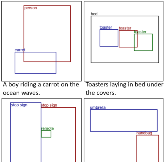
Figure 1: Samples from the USCOCO dataset.

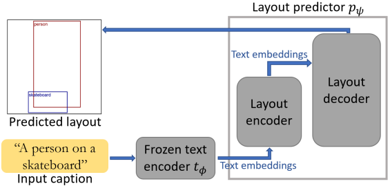
Figure 2: Overview of text-to-layout prediction.

2 Related work

Implicit syntax in language and visio-linguistic models Deep learning has ruled out the need for feature engineering in natural language processing including the extraction of syntactical features. With the advent of contextualized language models pretrained on large text corpora Peters et al. (2018); Devlin et al. (2019) representations of words and sentences are dynamically computed. Several studies have evaluated syntactical knowledge embedded in language models through targeted syntactic evaluation, probing, and downstream natural language understanding tasks Hewitt and Manning (2019); Manning et al. (2020); Linzen and Baroni (2021); Kulmizev and Nivre (2021). Here we consider the task of visually imagining the situation expressed in a sentence and show that in case of unexpected situations that are unlikely to occur in the training data the performance of language models strongly decreases.

Probing compositional multimodal reasoning One of the findings of our work, that is, the failure of current models in sentence-to-layout prediction of unusual situations, are in line with recent text-image alignment test suites like Winoground Thrush et al. (2022) and VALSE Parcalabescu et al. (2022), that ask to correctly retrieve an image using grammatically varying captions. The benchmark of Gokhale et al. (2022) considers a generation setting, like us, however, they evaluate image generation (down to pixels), while ignoring the role of the language encoder. Moreover, their captions are automatically generated from object names and simple spatial relations, and hence only contain explicit spatial relations, whereas our USCOCO captions are modified human-written COCO captions and include implicit spatial relations.

Explicitly embedding syntax in language representations. Popa et al. (2021) use a tensor factorisation model for computing token embeddings that integrate dependency structures. In section 3.2.1 we discuss models that integrate a constituency parse tree Qian et al. (2021); Sartran et al. (2022) as we use them as encoders in the sentence-to-layout prediction task. They build on generative parsing approaches using recurrent neural networks (Dyer et al., 2016; Choe and Charniak, 2016).

Visual scene layout prediction Hong et al. (2018), Tan et al. (2018) and Li et al. (2019b) introduce layout predictors that are similar to our autoregressive model. They also train on the realistic COCO dataset and generate a dynamic number of objects, but they do not investigate the layout predictions. Other layout prediction methods require structured input like triplets or graphs instead of free-form text (Li et al., 2019a; Johnson et al., 2018; Lee et al., 2020), are confined to layouts of only 2 objects (Collell et al., 2021), are unconditional (Li et al., 2019b), work in simplified, non-realistic settings (Radevski et al., 2020; Lee et al., 2020) or focus on predicting positions for known objects and their relationships (Radevski et al., 2020).

3 Methods

3.1 Task definition

Given a natural language caption $C$, the task is to generate a layout $L$ that captures a spatial 2D visual arrangement of the objects that the caption describes. A layout $L=\{b_{i}\}_{i}=\{(o_{i},x_{i},y_{i},w_{i},h_{i})\}_{i}$ consists of a varying number of visual objects, each represented by a 5-tuple, where $o_{i}$ is a label from a category vocabulary (in this paper: one of the 80 COCO categories, e.g., “elephant”), and where $(x_{i},y_{i},w_{i},h_{i})$ refers to the bounding box for that object. The coordinates of the middle point of a box are $x_{i},y_{i}$, and $w_{i},h_{i}$ are the width and height. A caption $C$ consists of a number $N_{c}$ of word tokens $c_{i}$. Hence, we want to learn the parameters $\theta$ of a model $f_{\theta}$ that maps captions to layouts: $L=f_{\theta}(C)$.

Model overview We split the prediction problem into two parts. First, a text encoder $t_{\phi}$ computes (potentially structured) text embeddings $e_{j}$ for input word tokens $c_{i}$: $E=t_{\phi}(C)$. Second, a layout predictor $p_{\psi}$ predicts an embedding $v_{k}$ per visual object: $v_{k}=p_{\psi}(E)$. These are projected by a multilayer perceptron to a categorical probability distribution to predict object labels: $o_{k}\sim\text{softmax}(\text{MLP}^{\text{label}}(v_{k}))$. Regression ($\times 4$) is used for positions $b_{k}=(x_{k},y_{k},w_{k},h_{k})$: e.g., $x_{k}=\sigma(\text{MLP}^{\text{pos}}(v_{k})_{x})$, with $\sigma:\mathbb{R}^{d}\mapsto[0,1]$ a sigmoid.

3.2 Text encoders $t_{\phi}$

We consider two types of text encoders. First, we explicitly encode the syntactical structure of a sentence in its semantic representation. As syntactical structure we choose a constituency parse as it naturally represents the structure of human language, and phrases can be mapped to visual objects. Human language is characterized by recursive structures which correspond with the recursion that humans perceive in the world Hawkings (2021); Hauser et al. (2002). Second, we encode the sentence with a state-of-the-art sentence encoder that is pretrained with a next token prediction objective. We assume that they implicitly encode syntax (Tenney et al., 2019; Warstadt et al., 2020). The choice of the next-token prediction objective is motivated by existing work that compares language models with implicit vs. explicit syntax (Qian et al., 2021; Sartran et al., 2022). We use pretrained text encoders, which are all frozen during layout prediction training to allow a clean comparison.

3.2.1 Explicitly embedding syntax in sentence representations

The models that explicitly embed syntax take a linearized version of the constituency trees as input, using brackets and constituent tags as tokens in addition to the input sentence $C$, to end up with $C^{\text{lin}}$. For instance, “A dog catches a frisbee” would be preprocessed into “(NP a dog) (VP catches (NP a frisbee))”. The constituency trees are obtained with the parser of Kitaev and Klein (2018); Kitaev et al. (2019). The model computes an embedding $e^{\text{struct}}_{j}\ (0\leq j<N_{c}+N_{\text{lin}})$ per input token $c_{j}$ (including the parentheses and syntax tags). The embeddings are given as is to the layout predictor, and since tokens explicitly representing structure (parentheses, syntax tags) have their own embedding, we assume the sequence of $e^{\text{struct}}_{j}$ to carry more structural information than the sequence formed by $e^{\text{base}}_{i}$ (cfr. section 3.2.2). We consider the following models, which are all pretrained on the BLLIP_LG dataset (Charniak et al., 2000, $\approx$40M tokens).

PLM: The Parsing as Language Model from Qian et al. (2021) inputs $C^{\text{lin}}$ into an untrained GPT-2 model and learns $e^{\text{struct}}_{j}$ by training on a next token prediction task.

PLM_mask: of Qian et al. (2021) is similar to PLM but uses masking to constrain two of the attention heads in the transformer layers to attend to tokens that are respectively part of the current constituent and part of the rest of the partially parsed sentence.

TG: The Transformer Grammars model from Sartran et al. (2022) uses a masking scheme that constrains all attention heads to only attend to local parts of the constituent tree. This results in a recursive composition of the representations of smaller constituents into the representations of larger constituents, which reflects closely the recursive property of Recurrent Neural Network Grammars (RNNG) models (Dyer et al., 2016). We adapt this model to use a GPT-2 backbone and we train it for next token prediction on the same dataset as the PLM models for a fair comparison.

TG_RB: To test to what extent differences in layout prediction performance are due to the explicit use of a constituency grammar, and not a byproduct of model and/or input differences, this model uses trivial right-branching constituency trees (constructed by taking the silver trees and moving all closing brackets to the end of the sentence), instead of silver constituency trees, both during pretraining and during layout generation. This model is also used by Sartran et al. (2022) as ablation baseline.

3.2.2 Baselines that are assumed to implicitly encode syntax

The baselines take a sequence of text tokens $c_{i}\ (0\leq i<N_{c})$ and produce a sequence of the same length, of embeddings $e^{\text{base}}_{i}\ (0\leq i<N_{c})$, which will be given to the layout decoder.

GPT-2_Bllip: This language model is also used by Qian et al. (2021) and shares its architecture and training regime with GPT-2 (Radford et al., 2019). It is trained on the sentences (not the linearized parse trees) of the BLLIP_LG dataset to predict the next token given the history (Charniak et al., 2000). Hence, this model is trained on the same sentences as the models of section 3.2.1. Even though it is debatable whether transformers can learn implicit syntax from the relatively small ($\approx$40M tokens) BLLIP_LG dataset, this model is used as baseline by existing work on explicit syntax in language modelling (Qian et al., 2021; Sartran et al., 2022), which is why we also include it. Furthermore, there is evidence that pretraining datasets of 10M-100M tokens suffice for transformers to learn most of their syntax capabilities Pérez-Mayos et al. (2021); Zhang et al. (2021); Samuel et al. (2023), even though orders of magnitude ($>$1B) more pretraining tokens are required for more general downstream NLU tasks.

GPT-2: As published by Radford et al. (2019), trained for next token prediction on a large-scale scraped webtext dataset.

$\textbf{GPT-2}_{\text{Bllip}}^{\text{shuffle}}$: Identical to the GPT-2_Bllip model but the tokens in the input sentence are randomly shuffled, to test whether syntax has any contribution at all. The pretraining is exactly the same as GPT-2_Bllip, with the token order preserved.

LLaMA: Large state-of-the-art language models trained on massive amounts of text, we use the 7B and 33B model variants (Touvron et al., 2023).

3.3 Layout predictors $p_{\psi}$

3.3.1 Models

As a baseline we consider the layout prediction LSTM from Hong et al. (2018) and Li et al. (2019c), further referred to as ObjLSTM. This model does not perform well and it trains slowly because of the LSTM architecture, so we propose two novel layout predictors. The two models use the same transformer encoder, and differ in their transformer decoder architecture.

PAR: This decoding model is inspired by the DETR model for object detection of Carion et al. (2020). The decoder generates a number of objects in a single forward parallel pass, after first predicting the number of objects.

SEQ: This autoregressive model is similar to the language generating transformer of Vaswani et al. (2017), but decodes object labels and bounding boxes and not language tokens. It predicts an object per step until the end-of-sequence token is predicted, or the maximum length is reached. The model is similar to the layout decoder of Li et al. (2019c), but uses transformers instead of LSTMs.

3.3.2 Training

The PAR model

is trained analogous to Carion et al. (2020) and Stewart et al. (2016) by first computing the minimum cost bipartite matching between predicted objects $\hat{b}_{i}$ and ground-truth objects $b_{j}$ (as the ordering might differ), using the Hungarian algorithm Kuhn (2010), with differences in box labels, positions and overlaps as cost.

The SEQ model

is trained to predict the next visual object given the previous GT objects. The order of generation is imposed (by a heuristic: from large to small in area, after Li et al. (2019c)). The 1^st, 2^nd,… generated object is matched with the largest, 2^nd but largest,… ground-truth object.

The PAR and SEQ models apply the following losses to each matched pair of predicted box $\hat{b}_{i}$ and ground-truth box $b_{j}$.

A cross-entropy loss

$\mathcal{L}_{\text{label}}(\hat{b}_{i},{b}_{j})$ applied to the object labels.

A combination of regression losses

applied to the bounding box coordinates.

• An L1-loss $\mathcal{L}_{\text{L1}}(\hat{b}_{i},{b}_{j})$ applied to each of the dimensions of the boxes Carion et al. (2020).

• The generalized box IoU loss $\mathcal{L}_{\text{gIoU}}(\hat{b}_{i},{b}_{j})$ proposed by Rezatofighi et al. (2019), taking into account overlap of boxes.

• An L1-loss $\mathcal{L}_{\text{prop}}$ taking into account the proportion of box width and height.

• A loss $\mathcal{L}_{\text{rel}}$ equal to the difference between predicted and ground-truth predictions of relative distances between objects.

The following losses are not applied between matched predicted and ground-truth object pairs, but to the entire sequence of output objects at once.

A cross-entropy loss

$\mathcal{L}_{\text{len}}$ to the predicted number of object queries (PAR only).

A contrastive structural loss

to enforce in a novel way the grammatical structure found in the parse trees on the output, in our case the visual object embeddings $v_{k}$ that are computed by the layout predictor and that are used to predict the object boxes and their labels.

To calculate the loss, all nodes in the parse tree, that is, leaf nodes corresponding to word tokens, and parent and root nodes corresponding to spans of word tokens, are represented separately by a positional embedding $e_{j}^{\text{pos}}(0\leq j<2N_{c}-1)$ following Shiv and Quirk (2019). The positional embeddings are learnt, they are agnostic of the content of the word or word spans they correspond to, and they encode the path through the tree, starting from the root, to the given node.

In a contrastive manner the loss forces the visual object representations $v_{k}$ to be close to the positional embeddings $e^{\text{pos}}_{j}$, but far from those $\hat{e}^{\text{pos}}_{j}$ of other sentences in the minibatch. It maximizes the posterior probability that the set of visual object embeddings $V_{m}=\{v_{k}\}_{k}$ for sample $m$ are matched with the set of tree positional embeddings $E_{m}=\{e_{j}^{\text{pos}}\}_{j}$ for the same sample $m$, and vice versa: $\mathcal{L}_{\text{struct}}(m)=-\log P(E_{m}|V_{m})-\log P(V_{m}|E_{m})$. These probabilities are computed as a softmax over similarity scores $S(m,n)$ between samples in the batch, where the denominator of the softmax sums over tree positions or objects, resp.

The similarity score for 2 samples $m,n$ is computed as a log-sum-exp function of the cosine similarities between the $i$’th visual object $v_{i}^{m}$ of sample $m$ and a visually informed syntax tree context vector $c^{n}_{i}$ representing all tree positions $\{e^{n}_{j}\}_{j}$ of sample $n$. The context vector $c^{n}_{i}$ is computed with the attention mechanism of Bahdanau et al. (2015), with tree positional embeddings $\{e^{n}_{j}\}_{j}$ as keys and values, and visual embedding $v^{m}_{i}$ as query. The dot product between query $v^{m}_{i}$ and keys $\{e^{n}_{j}\}_{j}$ is first additionally normalized over the visual objects corresponding to a tree position, before the regular normalization over tree positions. These normalized dot products between keys and queries constitute a soft matching between visual objects and constituency tree node positions (note: only the positions, representing syntax and not semantics of the words, are represented by the tree positional embeddings). Since the model learns this mapping from the training signal provided by this loss, it is not necessary to manually specify which text spans are to be matched to which visual objects.

The loss has resemblance to the loss used by Xu et al. (2018), replacing their text embeddings by our visual object embeddings, and their visual embeddings by our syntax tree embeddings. Note that only the constituency parse of the input text and the output embeddings are needed. In this case, the output embeddings represent visual objects, but they are in general not confined to only represent visual objects, they could technically represent anything. Hence, the loss is not tied to layout generation in specific, and could be applied to any generation task conditioned on (grammatically) structured text, as tree positions are matched to output embeddings. This novel loss is completely independent of the text encoder and can be applied to a text encoder with explicit syntax input, or to a text encoder with implicit syntax (if a constituency parse of the input is available)..

The final loss

for one training sample is the sum of the above losses $\mathcal{L}$, with $(\hat{b}_{i},{b}_{j})$ matched pairs of predicted and GT objects, and each loss weighted by a different weight $\lambda$.

$$\mathcal{L}_{\text{total}} =\lambda_{\text{1}}\mathcal{L}_{\text{struct}}+\lambda_{\text{2}}\mathcal{L}_{\text{len}}$$

$$+\sum_{(i,j)}\Big{[}\lambda_{\text{3}}\mathcal{L}_{\text{label}}(\hat{b}_{i},{b}_{j})+\lambda_{\text{4}}\mathcal{L}_{\text{L1}}(\hat{b}_{i},{b}_{j})$$

$$+\lambda_{\text{5}}\mathcal{L}_{\text{gIoU}}(\hat{b}_{i},{b}_{j})+\lambda_{\text{6}}\mathcal{L}_{\text{prop}}(\hat{b}_{i},{b}_{j})$$

$$+\lambda_{\text{7}}\mathcal{L}_{\text{rel}}(\hat{b}_{i},{b}_{j})\Big{]}$$ (1)

3.4 Datasets

$t_{\phi}$	Train set	Regime
PLM	BLLIP sents, trees	NTP
PLMmask	BLLIP sents, trees	NTP
TG	BLLIP sents, trees	NTP
GPT-2Bllip	BLLIP sents	NTP
GPT-2	$\approx$8B text tokens	NTP
LLaMA	1.4T tokens	NTP

Table 1: Overview of the text encoders, their training data and training regimes. NTP stands for next-token prediction.

The text encoders are pretrained on datasets summarized in Table 1. We use COCO captions and instances (bounding boxes and labels, Lin et al., 2014) for training and testing the layout decoder. We use the 2017 COCO split with 118K training images and 5K validation images (both with 5 captions per image). The testing images are not usable as they have no captions and bounding box annotations. We randomly pick 5K images from the training data for validation and use the remaining 113K as training set $\mathcal{D}_{\text{train}}$. We use the 2017 COCO validation set as in-domain test set $\mathcal{D}_{\text{indom}}$. $\mathcal{D}_{\text{USCOCO}}$ is our test set of unexpected situations with 2.4K layouts and 1 caption per layout.

Collection of USCOCO

We used Amazon Mechanical Turk (AMT) to collect ground-truth (caption, layout)-pairs denoting situations that are unlikely to occur in the training data. We obtained this test set in three steps. In the first step, we asked annotators to link sentence parts of captions in $\mathcal{D}_{\text{indom}}$ to bounding boxes.

Second, we used a script to replace linked sentence parts in the captions with a random COCO category name ($o_{\text{new}}$, with a different COCO supercategory than the bounding box had that the sentence part was linked to). The script also replaces the bounding box that the annotators linked to the replaced sentence part in the first step, with a bounding box for an object of the sampled category $o_{\text{new}}$. We use 4 replacement strategies: the first keeps the original box merely replacing its label. The next 3 strategies also adjust the size of the box based on average dimensions of boxes with category $o_{\text{new}}$ in $\mathcal{D}_{\text{train}}$, relative to the size of the nearest other box in the layout. The 2^nd places the middle point of the new box on the middle point of the replaced box, the 3^rd at an equal x-distance to the nearest object box and the the 4^th at an equal y-distance to the nearest object.

In the third step, annotators were shown the caption with the automatically replaced sentence part and the 4 corresponding automatically generated layouts. They were asked to evaluate whether the new caption is grammatically correct, and which of the 4 layouts fits the caption best (or none). Each sample of step 2 was verified by 3 different annotators. Samples where at least 2 annotators agreed on the same layout and none of the 3 annotators considered the sentence as grammatically incorrect, were added to the final USCOCO dataset.

The USCOCO test set follows a very different distribution of object categories than $\mathcal{D}_{\text{train}}$. To show this we calculate co-occurrences of object categories in all images (weighted so that every image has an equal impact) of $\mathcal{D}_{\text{train}}$, $\mathcal{D}_{\text{USCOCO}}$ and $\mathcal{D}_{\text{indom}}$. The co-occurence vectors of $\mathcal{D}_{\text{train}}$ and $\mathcal{D}_{\text{USCOCO}}$ have a cosine similarity of $47\%$, versus $99\%$ for $\mathcal{D}_{\text{train}}$ and the in-domain test set $\mathcal{D}_{\text{indom}}$.

3.5 Preprocessing of the images

Spurious bounding boxes (SP)

Because objects annotated with bounding boxes in the COCO images are not always mentioned in the corresponding captions, we implement a filter for bounding boxes and apply it on all train and test data. The filter computes for each object class $O$ of COCO the average diagonal length $\bar{d}_{O}$ of its bounding box, over the training set, and the normalized average diagonal length $\bar{d}^{\text{norm}}_{O}$ (scaled by the size of the biggest object of each image). Only the biggest object of a class per image is included in these averages to limit the influence of background objects. Then, all the objects with size smaller than $0.5\cdot\bar{d}_{O}$ and normalized size smaller than $0.5\cdot\bar{d}^{\text{norm}}_{O}$ are discarded. The normalized threshold allows the filters to be scale invariant, while the non-normalized threshold removes filtering mistakes when there is a big unimportant, unmentioned object in the image.

Crop-Pad-Normalize (CPN)

To center and scale bounding boxes, we follow Collell et al. (2021). We first crop the tightest enclosing box that contains all object bounding boxes. Then, we pad symmetrically the smallest side to get a square box of height and width $P$. This preserves the aspect ratio when normalizing. Finally, we normalize coordinates by $P$, resulting in coordinates in $[0,1]$.

3.6 Evaluation metrics

Pr, Re, F1

precision, recall and F1 score of predicted object labels, without taking their predicted bounding boxes into account.

$\boldsymbol{\text{Pr}_{0.5}}$, $\boldsymbol{\text{Re}_{0.5}}$, $\boldsymbol{\text{F1}_{0.5}}$

precision, recall and F1 score of predicted object labels, with an Intersection over Union (IoU) threshold of 0.5 considering the areas of the predicted and ground-truth bounding boxes (Ren et al., 2017). The matching set $M_{IoU}$ between ground-truth (GT) and predicted objects is computed in a greedy fashion based on box overlap in terms of pixels.

$\boldsymbol{\text{Re}^{\text{repl}}}$

The recall (without positions) on only the set of GT objects that have been replaced in the test set of unexpected situations $\mathcal{D}_{\text{USCOCO}}$.

	$\mathcal{D}_{\text{indom}}$			$\mathcal{D}_{\text{USCOCO}}$
	F1${}_{0.5}\uparrow$	F1 $\uparrow$	$\text{F1}_{Dpw}\uparrow$	F1${}_{0.5}\uparrow$	F1 $\uparrow$	$\text{F1}_{Dpw}\uparrow$
ObjLSTM*	.185 $\pm$ .021	.676 $\pm$ .006	.356 $\pm$ .019	.099 $\pm$ .013	.524 $\pm$ .009	.16 $\pm$ .019
ObjLSTMlrg + GPT-2Bllip	.104 $\pm$ .003	.542 $\pm$ .01	.238 $\pm$ .013	.074 $\pm$ .003	.404 $\pm$ .014	.078 $\pm$ .007
ObjLSTMlrg + GPT-2Bllip	.167 $\pm$ .005	.65 $\pm$ .006	.345 $\pm$ .01	.1 $\pm$ .003	.524 $\pm$ .016	.174 $\pm$ .019
SEQ + GPT-2Bllip	.271 $\pm$ .004	.597 $\pm$ .01	.304 $\pm$ .011	.167 $\pm$ .001	.485 $\pm$ .006	.149 $\pm$ .007
PAR + GPT-2Bllip	.296 $\pm$ .004	.67 $\pm$ .014	.375 $\pm$ .018	.18 $\pm$ .001	.576 $\pm$ .026	.229 $\pm$ .036
SEQ + TG	.28 $\pm$ .002	.638 $\pm$ .006	.344 $\pm$ .011	.177 $\pm$ .002	.541 $\pm$ .002	.203 $\pm$ .004
PAR + TG	.306 $\pm$ .008	.69 $\pm$ .002	.398 $\pm$ .008	.185 $\pm$ .004	.6 $\pm$ .004	.255 $\pm$ .005

Table 2: PAR, SEQ and ObjLSTM (baseline) layout predictor results on USCOCO and $\mathcal{D}_{\text{indom}}$, incl. F1, $\text{F1}_{0.5}$ and $\text{F1}_{Dpw}$ showing that the PAR decoding model performs best. All entries use the GPT-2_Bllip or TG text encoder (without structural loss), except for ObjLSTM* which uses a multimodal text encoder trained on images and text (Li et al., 2019c; Xu et al., 2018). ObjLSTM_lrg is scaled up to same number of parameters as SEQ and PAR, and uses a layout predictor with a transformer encoder before the LSTM decoder, like SEQ and PAR. Best results of models using implicit syntax (upper rows) and those with explicit syntax (lower rows, with TG) are marked in bold.

$\boldsymbol{\text{Pr}_{Dpw}}$, $\boldsymbol{\text{Re}_{Dpw}}$, $\boldsymbol{\text{F1}_{Dpw}}$

The $\text{F1}_{0.5}$ score penalizes an incorrect/missing label as much as it penalizes an incorrect position, while we consider an incorrect/missing label to be a worse error. Additionally, there are many plausible spatial arrangements for one caption (as explained in section 3.5 image preprocessing tries to reduce its impact). For this reason we introduce an F1 score based on the precision and recall of object pairs, penalized by the difference of the distance between the two boxes in the GT and the two boxes in the predictions. This metric penalizes incorrect positions, since a pair’s precision or recall gets downweighted when its distance is different from its distance in the GT, but it penalizes incorrect labels more, since pairs with incorrect labels have precision/recall equal to 0. Moreover, it evaluates positions of boxes relative to each other, instead of to one absolute GT layout.

First, a greedy matching set $M_{D}$ between GT and predicted objects is computed based on labels and middle-point distance. Boxes $\hat{b}$ are part of the predicted layout $L_{\text{p}}$ (with $N_{\text{p}}$ object pairs), and boxes $b$ are part of the GT layout $L_{\text{GT}}$ (with $N_{\text{GT}}$ object pairs). The matching function $\pi(\hat{b}_{i},\hat{b}_{k})$ equals 1 if predicted boxes $\hat{b}_{i}$ and $\hat{b}_{k}$ both have a matching box $b_{j}$ and $b_{m}$ in the GT (so $(i,j)\in M_{D}$ and $(k,m)\in M_{D}$), and equals 0 otherwise. $D$ denotes Euclidean distance between box middle points, and $S_{jm,ik}\in[0,1]$ is a normalized similarity metric based on this distance. The penalized precision $\text{Pr}_{Dpw}$ and recall $\text{Re}_{Dpw}$ are computed as follows:

$$S_{jm,ik} =1-\frac{1}{\sqrt{2}}|{D}(b_{j},b_{m})-{D}(\hat{b}_{i},\hat{b}_{k})|$$

$$\text{Pr}_{Dpw} =\frac{1}{N_{\text{p}}}\sum_{i\in L_{\text{p}}}\sum_{k\in L_{\text{p}}\setminus\{i\}}S_{jm,ik}\,\pi(\hat{b}_{i},\hat{b}_{k})$$ (2)

$$\text{Re}_{Dpw} =\frac{1}{N_{\text{GT}}}\sum_{i\in L_{\text{p}}}\sum_{k\in L_{\text{p}}\setminus\{i\}}S_{jm,ik}\,\pi(\hat{b}_{i},\hat{b}_{k})$$ (3)

where $$(i,j)\in M_{D}\ \text{and}\ (k,m)\in M_{D}.$$

${\text{F1}_{Dpw}}$ is finally computed as the standard F1 of ${\text{Pr}_{Dpw}}$ and ${\text{Re}_{Dpw}}$. If a sample has less than 2 boxes in the GT or predictions, respectively ${\text{Re}_{Dpw}}$ or ${\text{Pr}_{Dpw}}$ is undefined for that sample.

4 Experiments

4.1 Experimental set-up

All runs were repeated three times and the averages and standard deviations are reported. We used a learning rate of $10^{-4}$ with Adam (Kingma and Ba, 2015), a batch size of 128 (64 for runs using $\mathcal{L}_{\text{struct}}$), random horizontal flips on the bounding boxes as data augmentation, and early stopping. All text encoders were frozen. Layout predictors use a hidden dimension of 256 and a FFN dimension of 1024, with 4 encoder layers and 6 decoder layers, and have 10M parameters. The loss weights (eq. 3.3.2) were chosen experimentally and set to $\lambda_{\text{1}}\in\{0.25,0.5,1.0\}$, $\lambda_{\text{2}}=0.1$, $\lambda_{\text{3}}=0.5$, $\lambda_{\text{4}}=5$, $\lambda_{\text{5}}=2$, $\lambda_{\text{6}}=0.5$, $\lambda_{\text{7}}=0.5$. We took most of the other PAR hyperparameters from Carion et al. (2020). We run all text encoders with the smallest GPT-2 architecture (125M params), for which we reuse checkpoints shared by Qian et al. (2021) for PLM, PLM_mask and GPT-2_Bllip. We also run GPT-2-lg_Bllip, GPT-2-lg and TG-lg with the larger GPT-2 architecture (755M params). GPT-2 and GPT-2-lg runs use checkpoints from Huggingface Wolf et al. (2020), and LLaMA runs use checkpoints shared by Meta. We train GPT-2-lg_Bllip ourselves, using the code of Qian et al. (2021). Models were trained on one 16GB Tesla P100 or 32GB Tesla V100 GPU (except the LLaMA-33B runs which were trained on a 80GB A100).

Training TG

We train TG and TG-lg like PLM and baseline GPT-2_Bllip following Qian et al. (2021), with a learning rate $10^{-5}$, the AdamW optimizer, a batch size of 5 and trained until convergence on the development set of the BLLIP_LG dataset split (Charniak et al., 2000). We implement TG with the recursive masking procedure of Sartran et al. (2022), but without the relative positional encodings, since these do not contribute much to the performance, and because GPT-2 uses absolute position embeddings.

			$\mathcal{D}_{\text{USCOCO}}$
		Size	$\text{F1}_{Dpw}\uparrow$	$\text{F1}_{0.5}\uparrow$	F1 $\uparrow$
GPT-2		125M	.207 $\pm$ .019	.179 $\pm$ .008	.566 $\pm$ .02
GPT-2	+ $\mathcal{L}_{\text{struct}}$		.187 $\pm$ .006	.184 $\pm$ .007	.555 $\pm$ .011
GPT-2Bllip			.229 $\pm$ .036	.18 $\pm$ .001	.576 $\pm$ .026
GPT-2Bllip	+ $\mathcal{L}_{\text{struct}}$		.233 $\pm$ .014	.192 $\pm$ .003	.574 $\pm$ .014
GPT-2-lg		755M	.283 $\pm$ .047	.188 $\pm$ .005	.61 $\pm$ .03
GPT-2-lg	+ $\mathcal{L}_{\text{struct}}$		.292 $\pm$ .025	.205 $\pm$ .009	.628 $\pm$ .016
GPT-2-lgBllip			.233 $\pm$ .027	.183 $\pm$ .002	.586 $\pm$ .019
GPT-2-lgBllip	+ $\mathcal{L}_{\text{struct}}$		.234 $\pm$ .019	.196 $\pm$ .005	.579 $\pm$ .006
LLaMA-7B		7B	.231 $\pm$ .014	.179 $\pm$ .007	.583 $\pm$ .011
LLaMA-7B	+ $\mathcal{L}_{\text{struct}}$		.26 $\pm$ .026	.192 $\pm$ .01	.602 $\pm$ .02
PLM		125M	.226 $\pm$ .006	.18 $\pm$ .002	.579 $\pm$ .002
PLM	+ $\mathcal{L}_{\text{struct}}$		.282 $\pm$ .048	.192 $\pm$ .002	.61 $\pm$ .033
PLMmask			.234 $\pm$ .012	.176 $\pm$ .005	.588 $\pm$ .01
PLMmask	+ $\mathcal{L}_{\text{struct}}$		.28 $\pm$ .039	.191 $\pm$ .007	.612 $\pm$ .024
TG			.255 $\pm$ .005	.185 $\pm$ .004	.6 $\pm$ .004
TG	+ $\mathcal{L}_{\text{struct}}$		.318 $\pm$ .026	.192 $\pm$ .008	.641 $\pm$ .018
TG-lg		755M	.283 $\pm$ .017	.183 $\pm$ .008	.621 $\pm$ .014
TG-lg	+ $\mathcal{L}_{\text{struct}}$		.327 $\pm$ .018	.195 $\pm$ .006	.645 $\pm$ .01

Table 3: Text encoders with implicit (above double line) and explicit (below double line) syntax, and structural loss results on USCOCO: F1, precision and recall, with and without IoU threshold and pairwise distance weighted. All entries use the PAR layout predictor. Results of the best (in terms of $\text{F1}_{Dpw}$) $\lambda_{\text{1}}$ for each model type are shown.

5 Results and discussion

5.1 Layout prediction

5.1.1 Preprocessing of images

We ran a comparison of preprocessing for the PLM and GPT-2_Bllip text encoders (both using PAR). All conclusions were identical. Using SP gives small but significant improvements in F1_0.5 and F1 on both test sets, and larger improvements when also normalizing bounding boxes with CPN. Using CPN increases the position sensitive F1_0.5 metric drastically on both test sets, even more so when also using SP. In a human evaluation with AMT, annotators chose the best layout given a COCO caption from $\mathcal{D}_{\text{indom}}$. 500 captions with 2 corresponding layouts (one from $\mathcal{D}_{\text{indom}}$ + CPN + SP and one from $\mathcal{D}_{\text{indom}}$ + CPN) were evaluated by 3 annotators, who preferred SP in 37% of cases, as opposed to 18.6% where they preferred not using SP (44.4% of the time they were indifferent). These results suggest that the preprocessing techniques improve the alignment of COCO bounding boxes with their captions, and that the best alignment is achieved when using both.

5.1.2 Layout prediction models

Table 2 compares our new PAR and SEQ layout predictors with the ObjLSTM baseline. All models use either the GPT-2_Bllip or TG text encoder (based on the small GPT-2 architecture), except for ObjLSTM* which uses a multimodal text encoder following Li et al. (2019c); Xu et al. (2018). The $\mathcal{L}_{\text{rel}}$ and $\mathcal{L}_{\text{prop}}$ losses are used for the SEQ and PAR runs (in Table 2 and subsequent Tables). These losses give minor consistent improvements in $\text{F1}_{0.5}$, while keeping F1 more or less constant.

Both SEQ / PAR + GPT-2_Bllip models outperform all ObjLSTM baselines by significant margin on the position sensitive $\text{F1}_{0.5}$ metric on both test sets (even though ObjLSTM* uses a text encoder that has been pretrained on multimodal data). PAR + GPT-2_Bllip obtains better $\text{F1}_{Dpw}$ and position insensitive F1 scores than baselines on the unexpected test set, and similar $\text{F1}_{Dpw}$ and F1 on $\mathcal{D}_{\text{indom}}$. SEQ + GPT-2_Bllip lags a bit behind on the last 2 metrics.

PAR obtains a significantly better precision than SEQ, both with and without object positions (Pr and $\text{Pr}_{0.5}$), on both test sets, both with GPT-2_Bllip and TG, resulting in greater F1 scores. This could be attributed to the fact that the $n$^th prediction with SEQ is conditioned only on the text and $n-1$ preceding objects, while with PAR, all predictions are conditioned on the text and on all other objects. The fact that for generating language, autoregressive models like SEQ are superior to non-autoregressive models like PAR, but vice versa for generating a set of visual objects, may be due to the inherent sequential character of language, as opposed to the set of visual objects in a layout, which does not follow a natural sequential order. When generating a set of objects in parallel, the transformer’s self-attention can model all pairwise relationships between objects before assigning any positions or labels. In contrast, when modelling a sequence of objects autoregressively, the model is forced to decide on the first object’s label and position without being able to take into account the rest of the generated objects, and it cannot change those decisions later on.

Since the PAR model scores higher and is more efficient (it decodes all $\hat{b}_{i}$ in one forward pass, compared to one forward pass per $\hat{b}_{i}$ for SEQ), we use PAR in subsequent experiments.

5.2 Improved generalization to USCOCO data with syntax

5.2.1 Explicitly modelling syntax

Table 3 shows layout prediction F1_0.5, F1 and $\text{F1}_{Dpw}$ on the USCOCO test set of PAR with implicitly structured GPT-2_Bllip, GPT-2 and LLaMA-7B text encoders (upper half) vs. with explicitly structured PLM, PLM_mask and TG text encoders (bottom half), with (rows with + $\mathcal{L}_{\text{struct}}$) and without ($\lambda_{\text{1}}=0$) structural loss.

Without structural loss, all smaller 125M models achieve very similar F1_0.5 scores compared to the baseline GPT-2_Bllip, and only TG is able to slightly improve the F1 and $\text{F1}_{Dpw}$ scores. We assume that models with explicit syntax, i.e., that integrate syntax in the input sentence, do not learn to fully utilize the compositionality of the syntax with current learning objectives.

We observe a noticeable increase over all metrics by using GPT-2-lg compared to GPT-2 which is to be expected, while GPT-2-lg_Bllip and GPT-2_Bllip perform equally where we assume that the training with a relatively small dataset does not fully exploit the capabilities of a larger model. TG-lg obtains similar scores as TG with a small increase for the $\text{F1}_{Dpw}$ and performs on par with GPT-2-lg while trained on only a fraction of the data.

Notable is that the very large LLaMA-7B model performs on par with GPT-2_Bllip and GPT-2-lg_Bllip. A possible explanation could be the quite drastic downscaling of the 4096-dimensional features of LLaMA-7B to 256 dimensions for our layout predictor by a linear layer. Using a 4096-dimensional hidden dimension for the layout predictor did not improve results. This increased the number of trainable parameters by two orders of magnitude, and the large resulting model possibly overfitted the COCO train set.

TG outperforms PLM and PLM_mask in F1 and $\text{F1}_{Dpw}$, which proves that restricting the attention masking scheme to follow a recursive pattern according to the recursion of syntax in the sentence helps generalizing to unexpected situations. This is in line with Sartran et al. (2022) who find that TG text encoders show better syntactic generalization.

5.2.2 Structural loss

Table 3 displays in the rows with + $\mathcal{L}_{\text{struct}}$ the impact of training with our structural loss function, with the best weight $\lambda_{\text{1}}$ in the total loss in eq. (3.3.2) chosen from $\{0.25,0.5,1.0\}$. $\text{F1}_{0.5}$ and $\text{Pr}_{0.5}$ slightly increase for all models and all $\lambda_{\text{1}}$ values. $\text{Re}_{0.5}$ is little affected, except for some explicit syntax models and LLaMA that see a slight increase.

F1, $\boldsymbol{\text{F1}_{Dpw}}$

For implicit syntax models, with increasing $\lambda_{\text{1}}$, Re and $\text{Re}_{Dpw}$ decrease severely. Pr and $\text{Pr}_{Dpw}$ first increase and then decrease again, resulting in sometimes stable but eventually decreasing F1 scores. For models with explicit syntax, Re and $\text{Re}_{Dpw}$ increase most for small loss weights ($\lambda_{\text{1}}=0.25$), while Pr and $\text{Pr}_{Dpw}$ top at $\lambda_{\text{1}}=0.5$ or $1.0$. Together this causes an improvement in F1 but mainly a sharp rise in $\text{F1}_{Dpw}$. These trends are more prominent for small models, but persist for large models, incl. LLaMA. $\text{F1}_{Dpw}$ peaks for TG/TG-lg with $0.25\cdot\mathcal{L}_{\text{struct}}$ at 0.318/0.327, which is a $\approx$40% increase of the baselines’ performance of GPT-2_Bllip/GPT-2-lg_Bllip at 0.229/0.233.

The loss, enforcing explicit constituency tree structure in the output visual embeddings, trains the layout predictor to not lose the explicit structure encoded by TG, PLM and PLM_mask. This compositional structure causes a disentangled, recursive representation of visual scenes Hawkings (2021); Hauser et al. (2002), facilitating the replacement of objects with unexpected different objects for input sentences that contain unexpected combinations of objects. For models with implicit syntax, the loss tries to enforce a structure that is not explicitly available in the models’ input (as opposed to for the models with explicit syntax), which may lead to a more difficult learning objective.

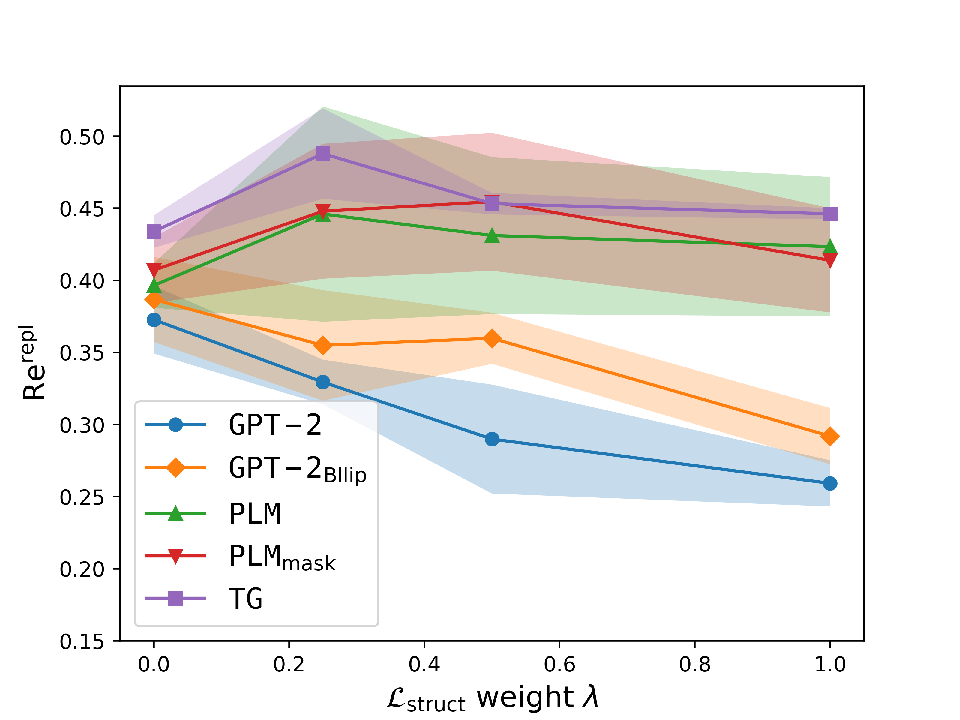
Figure 3: Recall on replaced objects $\text{Re}^{\text{repl}}$ in USCOCO vs. structural loss $\mathcal{L}_{\text{struct}}$ weight $\lambda_{\text{1}}$.

$\text{Re}^{\text{repl}}$

Figure 3 shows the recall $\text{Re}^{\text{repl}}$ on the replaced object of USCOCO (the unusual object). $\text{Re}^{\text{repl}}$ increases for models with explicit syntax, topping at $\lambda_{\text{1}}=0.25$, while it decreases sharply for models with implicit syntax GPT-2 and $\texttt{GPT-2}_{\text{Bllip}}$.

			$\mathcal{D}_{\text{indom}}$				$\mathcal{D}_{\text{USCOCO}}$
		Size	$\text{F1}_{0.5}\uparrow$	F1 $\uparrow$	$\text{F1}_{Dpw}\uparrow$		$\text{F1}_{0.5}\uparrow$	F1 $\uparrow$	$\text{F1}_{Dpw}\uparrow$
$\texttt{GPT-2}_{\text{Bllip}}^{\text{shuffle}}$		125M	.286 $\pm$ .006	.656 $\pm$ .005	.349 $\pm$ .012		.166 $\pm$ .002	.566 $\pm$ .003	.213 $\pm$ .004
GPT-2		125M	.294 $\pm$ .004	.66 $\pm$ .01	.353 $\pm$ .019		.179 $\pm$ .008	.566 $\pm$ .02	.207 $\pm$ .019
GPT-2Bllip			.296 $\pm$ .004	.67 $\pm$ .014	.375 $\pm$ .018		.18 $\pm$ .001	.576 $\pm$ .026	.229 $\pm$ .036
GPT-2-lg		755M	.308 $\pm$ .001	.702 $\pm$ .007	.414 $\pm$ .013		.188 $\pm$ .005	.61 $\pm$ .03	.283 $\pm$ .047
GPT-2-lgBllip			.298 $\pm$ .004	.676 $\pm$ .01	.38 $\pm$ .013		.183 $\pm$ .002	.586 $\pm$ .019	.233 $\pm$ .027
LLaMA-7B		7B	.306 $\pm$ .001	.701 $\pm$ .003	.411 $\pm$ .008		.179 $\pm$ .007	.583 $\pm$ .011	.231 $\pm$ .014
LLaMA-33B		33B	.305 $\pm$ .005	.699 $\pm$ .003	.406 $\pm$ .002		.181 $\pm$ .006	.577 $\pm$ .008	.225 $\pm$ .011
TGRB		125M	.299 $\pm$ .005	.683 $\pm$ .01	.391 $\pm$ .015		.178 $\pm$ .004	.571 $\pm$ .011	.216 $\pm$ .016
TGRB	+ $\mathcal{L}_{\text{struct}}$		.3 $\pm$ .005	.67 $\pm$ .01	.358 $\pm$ .012		.189 $\pm$ .007	.606 $\pm$ .017	.278 $\pm$ .02
PLM	+ $\mathcal{L}_{\text{struct}}$	125M	.301 $\pm$ .006	.677 $\pm$ .022	.378 $\pm$ .038		.192 $\pm$ .002	.61 $\pm$ .033	.282 $\pm$ .048
PLMmask	+ $\mathcal{L}_{\text{struct}}$		.3 $\pm$ .004	.683 $\pm$ .003	.388 $\pm$ .007		.191 $\pm$ .007	.612 $\pm$ .024	.28 $\pm$ .039
TG	+ $\mathcal{L}_{\text{struct}}$		.305 $\pm$ .005	.685 $\pm$ .012	.379 $\pm$ .028		.192 $\pm$ .008	.641 $\pm$ .018	.318 $\pm$ .026
TG-lg	+ $\mathcal{L}_{\text{struct}}$	755M	.306 $\pm$ .004	.692 $\pm$ .002	.392 $\pm$ .007		.195 $\pm$ .006	.645 $\pm$ .01	.327 $\pm$ .018

Table 4: Final model results in terms of F1, $\text{F1}_{0.5}$, and $\text{F1}_{Dpw}$ on the in-domain (left) and USCOCO (right) test sets. All entries use the PAR layout predictor, and explicit syntax models use $\lambda_{\text{1}}=0.25$ or $\lambda_{\text{1}}=0.50$. GPT-2(-lg) and LLaMA have been pretrained on much larger text datasets.

5.2.3 Overview of explicit vs. implicit syntax

Table 4 gathers results on both test sets. The results for all models, but most notably the implicit syntax models, drop significantly on USCOCO compared to $\mathcal{D}_{\text{indom}}$, confirming that current state-of-the-art models struggle with generating unexpected visual scenes.

$\mathcal{D}_{\text{indom}}$

Small models that explicitly model syntax obtain slightly better results than the small baseline models for all metrics. Models with implicit syntax might perform well on in-domain test data because they have memorized the common structures in training data. The large models that were pretrained on huge text datasets (GPT-2-lg, LLaMA-xB) outperform TG-lg on $\mathcal{D}_{\text{indom}}$, showing that their pretraining does help for this task, but the drop in USCOCO scores suggests that they might overfit the memorized patterns. Situations described in COCO captions are commonly found in pretraining data, so that syntax is not needed to predict their visual layouts. The unexpected USCOCO situations however require the extra compositionality offered by explicit syntax.

USCOCO

We clearly see improvement in results of models that explicitly model syntax, showing the generalization capabilities needed to perform well on the unseen object combinations of USCOCO, provided it is enforced by a correct learning objective as discussed in section 5.2.2. This increase comes without a decrease in performance on the in-domain test data. This is important because it will lead to efficient models for natural language processing that can generalize to examples not seen in the training data, exploiting compositionality.

$\texttt{GPT-2}_{\text{Bllip}}^{\text{shuffle}}$

Another indication that the models that implicitly model syntax do not use the structure of natural language to the same extent, but rather exploit co-occurences in training data, is the fact that $\texttt{GPT-2}_{\text{Bllip}}^{\text{shuffle}}$, which is trained to generate layouts from sentences with shuffled words, achieves only slightly worse results than GPT-2_Bllip, even on the position sensitive $\text{F1}_{0.5}$ and $\text{F1}_{Dpw}$ metrics.

TG_RB

obtains similar scores to TG on in-domain data with trivial right-branching trees. On unexpected data, performance drops, proving the importance of syntax especially for generalizing to unexpected data. The structured loss improves generalization shown by USCOCO results, but not to the same extent as for TG.

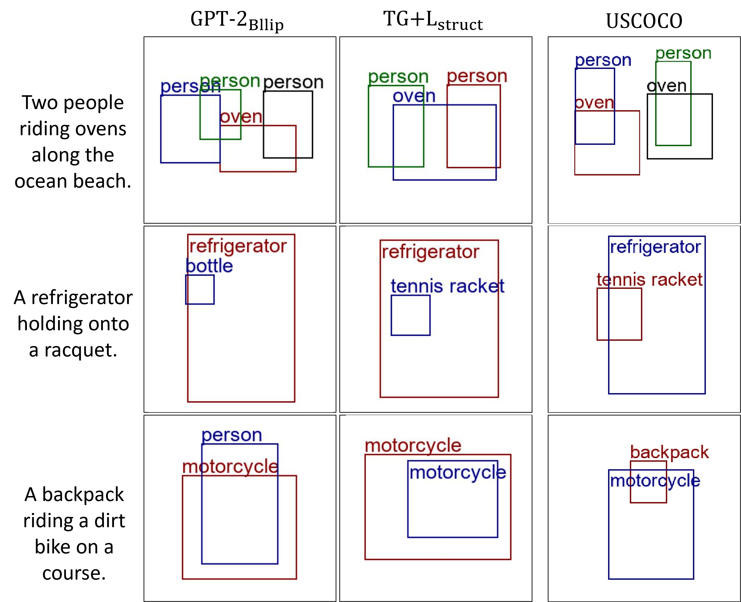
Figure 4: Examples of generated layouts where annotators chose the layout of TG + $\mathcal{L}_{\text{struct}}$ over the layout of $\texttt{GPT-2}_{\text{Bllip}}$ (first 2 examples) and vice versa (last example).

5.2.4 Human evaluation

Proper automatic evaluation of performance on the text-to-layout prediction task is hard, since potentially many spatial layouts may fit the scene described by a sentence. Our metrics compare the predictions to one single ground-truth, ignoring this fact, so we used AMT for a human evaluation of predicted layouts for 500 randomly sampled USCOCO captions. For each caption, 3 annotators chose the layout that best fit the caption from a pair of two, based on the following criteria: Whether the layout displays all objects present in the caption, whether the objects’ spatial arrangement corresponds to the caption, whether the objects have reasonable proportions and finally whether object predictions that are not explicitly mentioned in the caption do fit the rest of the scene (i.e., the only absurd or unexpected objects in the layout should be explicitly mentioned in the caption). Figure 4 shows some examples of generated layouts and the annotators’ decisions.

The results in Figure 5 are in line with the quantitative results where our structural loss proved beneficial for TG. This confirms that explicit structure does not improve layout prediction of unexpected combinations by itself, but together with our structural loss it causes a significant improvement. We calculated the agreement of the human evaluation with our quantitative metrics, and found 15.2% for $\text{F1}_{0.5}$, 41.7% for F1 and 42.5% for $\text{F1}_{Dpw}$. This confirms the previously mentioned suspicion that $\text{F1}_{0.5}$ is far less suitable for the evaluation of layout generation than F1 and $\text{F1}_{Dpw}$.

5.2.5 Constituency tree probes

To test how the loss affects syntax information in the text embeddings, we run a classifier probe inspired by Tenney et al. (2019) on the text encoder output and subsequent layers of the encoder of the layout prediction model. The probe classifies random spans of tokens as being a constituent or not (but ignores their tag).

Figure 6 shows that all text encoders’ outputs (probe layer 0) get good F1 scores and hence do encode syntax. Without the proposed structural loss, probing results quickly deteriorate in subsequent layers, presumably because the encoder has too little incentive to use and retain constituency structure, because COCO training data contains only situations common in pretraining data and requires no syntactical reasoning. The figure also shows that it is easier to predict constituency structure from outputs of text encoders with explicit syntax than of those with implicit syntax, which is not surprising because of the former’s pretraining and the presence of parentheses and tags.

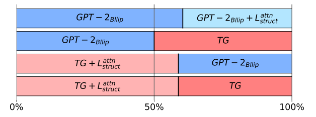
Figure 5: Human evaluation of generated layouts by GPT-2_Bllip (+ $\mathcal{L}_{\text{struct}}$) and TG (+ $\mathcal{L}_{\text{struct}}$) on USCOCO. Annotators choose the best layout between 2 layouts (anonymized and order-randomized).

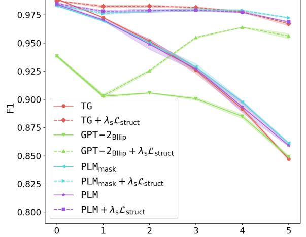
Figure 6: Constituency tree probe results for $\texttt{GPT-2}_{\text{Bllip}}$, TG, PLM and PLM_mask on USCOCO. Layer 0 corresponds to text encoder output (with model-dependent dimensions), layer 1 to the 256-dimensional embedding after linear projection, layer 2 to the output of the 1^st encoder layer, etc.

The structural loss helps to almost perfectly retain the constituency structure. The loss matches the output (in our case visual objects) to constituency tree positions, and as the probe shows, to do so, it propagates the constituency tree information present in the text through the model. For GPT-2_Bllip, except for an initial drop caused by the linear projection to a lower dimension, the loss improves probing F1 in later layers, even beyond the F1 for raw text encoder output. That this increase does not lead to improved layout predictions could be explained by the relevant syntax being encoded in a different, more implicit form that is harder for downstream models to learn to use.

5.2.6 Computational cost

The addition of structural (parenthesis and tag) tokens to explicit syntax model input causes the number of tokens $N_{c}+N_{\text{lin}}$ to be larger than the number of tokens $N_{c}$ that implicit models use to encode the same sentence. GPT-2 needs only 11 tokens on average per sentence in the COCO validation set, versus TG that needs 38 and PLM that needs 30. This translates in a greater computational cost for the explicit syntax models.

Nevertheless, the small TG + $\mathcal{L}_{\text{struct}}$, pretrained only on BLLIP_LG, outperforms the large GPT-2-lg that has been pretrained on a much larger dataset. This entails multiple computational advantages: smaller memory footprint and fewer resources and less time needed for pretraining.

6 Limitations & future work

One limitation of layout decoding with explicitly structured language models is the reliance upon a syntax parsing model to obtain the constituency trees for input captions. While syntax parsing models have shown very high performance (the parser of Kitaev and Klein (2018) obtains an F1 score of 95.13 on the Penn Treebank (Marcus et al., 1993), which contains longer and more syntactically complex sentences than typical COCO captions), grammatical errors in the used prompts might result in incorrect parses and hence in worse layout generations, compared to language models without explicit syntax (that do not need a parser). We leave an investigation into this phenomenon for further research. However, we do note an increased performance of layout generation even with only trivial right-branching trees over implicit syntax models (visible in Table 4), which might be an indication of robustness against grammatical errors for models that explicitly encode syntax.

Furthermore, while we show that explicitly modelling syntax improves layout prediction for absurd situations, this out-of-distribution generation task still remains difficult even for the best layout predictor models: there is a 35-37% drop in F1 score and 17-26% drop in $\text{F1}_{Dpw}$ on USCOCO compared to the in-domain test set. The introduction of USCOCO allows further research to evaluate new layout generation models on their out-of-distribution and absurd generation capabilities.

Very recent work has prompted the GPT-4 API to generate SVG or TikZ code that can be rendered into schematic images, which can then be used to guide the generation of more detailed images (Bubeck et al., 2023; Zhang et al., 2023). The layout prediction models discussed in our paper generate bounding box coordinates and class labels, which are hard to directly compare to code or rendered images. Moreover, we studied the role that explicit grammar can play for robustness with respect to absurd inputs, which would not have been possible with the GPT-4 API. However, using LLMs for layout prediction can be a promising direction for future work.

7 Conclusion

We evaluated models that implicitly and explicitly capture the syntax of a sentence and assessed how well they retain this syntax in the representations when performing the downstream task of layout prediction of objects on a 2D canvas. To test compositional understanding, we collected a test set of grammatically correct sentences and layouts describing compositions of entities and relations that unlikely have been seen during training. We introduced a novel parallel decoder for layout prediction based on a transformer architecture, but most importantly we proposed a novel contrastive structural loss that enforces the encoding of syntax structure in the representation of a visual scene and show that it increases generalization to unexpected compositions resulting in large performance gains in the task of 2D spatial layout prediction conditioned on text. The loss has the potential to be used in other generation tasks that condition on structured input, which could be investigated in future work. Our research is a step forward in retaining structured knowledge in neural models.

References

- Bahdanau et al. (2015) Dzmitry Bahdanau, Kyunghyun Cho, and Yoshua Bengio. 2015. Neural machine translation by jointly learning to align and translate. In 3rd International Conference on Learning Representations, ICLR.
- Bubeck et al. (2023) Sébastien Bubeck, Varun Chandrasekaran, Ronen Eldan, Johannes Gehrke, Eric Horvitz, Ece Kamar, Peter Lee, Yin Tat Lee, Yuanzhi Li, Scott M. Lundberg, Harsha Nori, Hamid Palangi, Marco Túlio Ribeiro, and Yi Zhang. 2023. Sparks of artificial general intelligence: Early experiments with GPT-4. CoRR, abs/2303.12712.
- Carion et al. (2020) Nicolas Carion, Francisco Massa, Gabriel Synnaeve, Nicolas Usunier, Alexander Kirillov, and Sergey Zagoruyko. 2020. End-to-end object detection with transformers. In Computer Vision - ECCV 2020 - 16th European Conference, volume 12346 of Lecture Notes in Computer Science, pages 213–229. Springer.
- Charniak et al. (2000) Eugene Charniak, Don Blaheta, Niyu Ge, Keith Hall, John Hale, and Mark Johnson. 2000. Bllip 1987-89 wsj corpus release 1 ldc2000t43.
- Chen et al. (2023) Minghao Chen, Iro Laina, and Andrea Vedaldi. 2023. Training-free layout control with cross-attention guidance. CoRR, abs/2304.03373.
- Choe and Charniak (2016) Do Kook Choe and Eugene Charniak. 2016. Parsing as language modeling. In Proceedings of the 2016 Conference on Empirical Methods in Natural Language Processing, EMNLP, pages 2331–2336. The Association for Computational Linguistics.
- Chomsky (1965) Noam Chomsky. 1965. Aspects of the Theory of Syntax. MIT press.
- Collell et al. (2021) Guillem Collell, Thierry Deruyttere, and Marie-Francine Moens. 2021. Probing spatial clues: Canonical spatial templates for object relationship understanding. IEEE Access, 9:134298–134318.
- Couairon et al. (2022) Guillaume Couairon, Jakob Verbeek, Holger Schwenk, and Matthieu Cord. 2022. Diffedit: Diffusion-based semantic image editing with mask guidance. CoRR, abs/2210.11427.
- Devlin et al. (2019) Jacob Devlin, Ming-Wei Chang, Kenton Lee, and Kristina Toutanova. 2019. BERT: pre-training of deep bidirectional transformers for language understanding. In Proceedings of the 2019 Conference of the North American Chapter of the Association for Computational Linguistics: Human Language Technologies, NAACL-HLT 2019, pages 4171–4186. Association for Computational Linguistics.
- Dyer et al. (2016) Chris Dyer, Adhiguna Kuncoro, Miguel Ballesteros, and Noah A. Smith. 2016. Recurrent neural network grammars. In NAACL HLT 2016, The 2016 Conference of the North American Chapter of the Association for Computational Linguistics: Human Language Technologies, San Diego California, USA, June 12-17, 2016, pages 199–209. The Association for Computational Linguistics.
- Frankland and Greene (2020) Steven M. Frankland and Joshua D. Greene. 2020. Concepts and compositionality: In search of the brain’s language of thought. Annual Review of Psychology, 71(1):273–303. PMID: 31550985.
- Geirhos et al. (2020) Robert Geirhos, Jörn-Henrik Jacobsen, Claudio Michaelis, Richard Zemel, Wieland Brendel, Matthias Bethge, and Felix A. Wichmann. 2020. Shortcut learning in deep neural networks. Nature Machine Intelligence, 2(11):665–673.
- Gokhale et al. (2022) Tejas Gokhale, Hamid Palangi, Besmira Nushi, Vibhav Vineet, Eric Horvitz, Ece Kamar, Chitta Baral, and Yezhou Yang. 2022. Benchmarking spatial relationships in text-to-image generation. CoRR, abs/2212.10015.
- Hauser et al. (2002) Marc D. Hauser, Noam Chomsky, and W. Tecumseh Fitch. 2002. The faculty of language: What is it, who has it, and how did it evolve? Science, 298(5598):1569–1579.
- Hawkings (2021) Jeff Hawkings. 2021. A Thousand Brains: A New Theory of Intelligence. Basic Books.
- Hewitt and Manning (2019) John Hewitt and Christopher D. Manning. 2019. A structural probe for finding syntax in word representations. In Proceedings of the 2019 Conference of the North American Chapter of the Association for Computational Linguistics: Human Language Technologies, NAACL-HLT, pages 4129–4138. Association for Computational Linguistics.
- Hong et al. (2018) Seunghoon Hong, Dingdong Yang, Jongwook Choi, and Honglak Lee. 2018. Inferring semantic layout for hierarchical text-to-image synthesis. In 2018 IEEE Conference on Computer Vision and Pattern Recognition, CVPR 2018, pages 7986–7994. IEEE Computer Society.
- Humboldt (1999) Wilhelm Humboldt. 1999. On language: On the diversity of human language construction and its influence on the mental development of the human species. Cambridge University Press.
- Johnson et al. (2018) Justin Johnson, Agrim Gupta, and Li Fei-Fei. 2018. Image generation from scene graphs. In 2018 IEEE Conference on Computer Vision and Pattern Recognition, CVPR, pages 1219–1228. Computer Vision Foundation / IEEE Computer Society.
- Kingma and Ba (2015) Diederik P. Kingma and Jimmy Ba. 2015. Adam: A method for stochastic optimization. In 3rd International Conference on Learning Representations, ICLR.
- Kitaev et al. (2019) Nikita Kitaev, Steven Cao, and Dan Klein. 2019. Multilingual constituency parsing with self-attention and pre-training. In Proceedings of the 57th Conference of the Association for Computational Linguistics, ACL, pages 3499–3505. Association for Computational Linguistics.
- Kitaev and Klein (2018) Nikita Kitaev and Dan Klein. 2018. Constituency parsing with a self-attentive encoder. In Proceedings of the 56th Annual Meeting of the Association for Computational Linguistics, ACL, pages 2676–2686. Association for Computational Linguistics.
- Kuhn (2010) Harold W. Kuhn. 2010. The hungarian method for the assignment problem. In Michael Jünger, Thomas M. Liebling, Denis Naddef, George L. Nemhauser, William R. Pulleyblank, Gerhard Reinelt, Giovanni Rinaldi, and Laurence A. Wolsey, editors, 50 Years of Integer Programming 1958-2008 - From the Early Years to the State-of-the-Art, pages 29–47. Springer.
- Kulmizev and Nivre (2021) Artur Kulmizev and Joakim Nivre. 2021. Schrödinger’s tree - on syntax and neural language models. CoRR, abs/2110.08887.
- Lee et al. (2020) Hsin-Ying Lee, Lu Jiang, Irfan Essa, Phuong B. Le, Haifeng Gong, Ming-Hsuan Yang, and Weilong Yang. 2020. Neural design network: Graphic layout generation with constraints. In Computer Vision - ECCV, volume 12348 of Lecture Notes in Computer Science, pages 491–506. Springer.
- Li et al. (2019a) Boren Li, Boyu Zhuang, Mingyang Li, and Jian Gu. 2019a. Seq-sg2sl: Inferring semantic layout from scene graph through sequence to sequence learning. In 2019 IEEE/CVF International Conference on Computer Vision, ICCV, pages 7434–7442. IEEE.
- Li et al. (2019b) Jianan Li, Jimei Yang, Aaron Hertzmann, Jianming Zhang, and Tingfa Xu. 2019b. Layoutgan: Generating graphic layouts with wireframe discriminators. In 7th International Conference on Learning Representations, ICLR. OpenReview.net.
- Li et al. (2019c) Wenbo Li, Pengchuan Zhang, Lei, Qiuyuan Huang, Xiaodong He, Siwei Lyu, and Jianfeng Gao. 2019c. Object-driven text-to-image synthesis via adversarial training. In IEEE Conference on Computer Vision and Pattern Recognition, CVPR 2019, pages 12174–12182. Computer Vision Foundation / IEEE.
- Lin et al. (2014) Tsung-Yi Lin, Michael Maire, Serge J. Belongie, James Hays, Pietro Perona, Deva Ramanan, Piotr Dollár, and C. Lawrence Zitnick. 2014. Microsoft COCO: common objects in context. In Computer Vision - ECCV 2014 - 13th European Conference, volume 8693 of Lecture Notes in Computer Science, pages 740–755. Springer.
- Linzen and Baroni (2021) Tal Linzen and Marco Baroni. 2021. Syntactic structure from deep learning. Annual Review of Linguistics, 7(1):195–212.
- Manning et al. (2020) Christopher D. Manning, Kevin Clark, John Hewitt, Urvashi Khandelwal, and Omer Levy. 2020. Emergent linguistic structure in artificial neural networks trained by self-supervision. Proc. Natl. Acad. Sci. USA, 117(48):30046–30054.
- Marcus et al. (1993) Mitchell P. Marcus, Beatrice Santorini, and Mary Ann Marcinkiewicz. 1993. Building a large annotated corpus of english: The penn treebank. Comput. Linguistics, 19(2):313–330.
- Parcalabescu et al. (2022) Letitia Parcalabescu, Michele Cafagna, Lilitta Muradjan, Anette Frank, Iacer Calixto, and Albert Gatt. 2022. VALSE: A task-independent benchmark for vision and language models centered on linguistic phenomena. In Proceedings of the 60th Annual Meeting of the Association for Computational Linguistics (Volume 1: Long Papers), ACL, pages 8253–8280. Association for Computational Linguistics.
- Pérez-Mayos et al. (2021) Laura Pérez-Mayos, Miguel Ballesteros, and Leo Wanner. 2021. How much pretraining data do language models need to learn syntax? In Proceedings of the 2021 Conference on Empirical Methods in Natural Language Processing, EMNLP, pages 1571–1582. Association for Computational Linguistics.
- Peters et al. (2018) Matthew E. Peters, Mark Neumann, Mohit Iyyer, Matt Gardner, Christopher Clark, Kenton Lee, and Luke Zettlemoyer. 2018. Deep contextualized word representations. In Proceedings of the 2018 Conference of the North American Chapter of the Association for Computational Linguistics: Human Language Technologies, NAACL-HLT, pages 2227–2237. Association for Computational Linguistics.
- Poole et al. (2022) Ben Poole, Ajay Jain, Jonathan T. Barron, and Ben Mildenhall. 2022. Dreamfusion: Text-to-3d using 2d diffusion. CoRR, abs/2209.14988.
- Popa et al. (2021) Diana Nicoleta Popa, Julien Perez, James Henderson, and Eric Gaussier. 2021. Towards syntax-aware token embeddings. Natural Language Engineering, 27(6):691–720.
- Qian et al. (2021) Peng Qian, Tahira Naseem, Roger Levy, and Ramón Fernandez Astudillo. 2021. Structural guidance for transformer language models. In Proceedings of the 59th Annual Meeting of the Association for Computational Linguistics and the 11th International Joint Conference on Natural Language Processing, ACL/IJCNLP, pages 3735–3745. Association for Computational Linguistics.
- Qu et al. (2023) Leigang Qu, Shengqiong Wu, Hao Fei, Liqiang Nie, and Tat-Seng Chua. 2023. Layoutllm-t2i: Eliciting layout guidance from llm for text-to-image generation.
- Radevski et al. (2020) Gorjan Radevski, Guillem Collell, Marie-Francine Moens, and Tinne Tuytelaars. 2020. Decoding language spatial relations to 2d spatial arrangements. In Proceedings of the 2020 Conference on Empirical Methods in Natural Language Processing: Findings, EMNLP 2020, Online Event, 16-20 November 2020, pages 4549–4560. Association for Computational Linguistics.
- Radford et al. (2021) Alec Radford, Jong Wook Kim, Chris Hallacy, Aditya Ramesh, Gabriel Goh, Sandhini Agarwal, Girish Sastry, Amanda Askell, Pamela Mishkin, Jack Clark, Gretchen Krueger, and Ilya Sutskever. 2021. Learning transferable visual models from natural language supervision. In Proceedings of the 38th International Conference on Machine Learning, ICML, volume 139 of Proceedings of Machine Learning Research, pages 8748–8763. PMLR.
- Radford et al. (2019) Alec Radford, Jeffrey Wu, Rewon Child, David Luan, Dario Amodei, Ilya Sutskever, et al. 2019. Language models are unsupervised multitask learners. OpenAI blog, 1(8):9.
- Ramesh et al. (2022) Aditya Ramesh, Prafulla Dhariwal, Alex Nichol, Casey Chu, and Mark Chen. 2022. Hierarchical text-conditional image generation with CLIP latents. CoRR, abs/2204.06125.
- Rassin et al. (2022) Royi Rassin, Shauli Ravfogel, and Yoav Goldberg. 2022. DALLE-2 is seeing double: Flaws in word-to-concept mapping in text2image models. In Proceedings of the Fifth BlackboxNLP Workshop on Analyzing and Interpreting Neural Networks for NLP, BlackboxNLP@EMNLP 2022, pages 335–345. Association for Computational Linguistics.
- Ren et al. (2017) Shaoqing Ren, Kaiming He, Ross B. Girshick, and Jian Sun. 2017. Faster R-CNN: towards real-time object detection with region proposal networks. IEEE Trans. Pattern Anal. Mach. Intell., 39(6):1137–1149.
- Rezatofighi et al. (2019) Hamid Rezatofighi, Nathan Tsoi, JunYoung Gwak, Amir Sadeghian, Ian D. Reid, and Silvio Savarese. 2019. Generalized intersection over union: A metric and a loss for bounding box regression. In IEEE Conference on Computer Vision and Pattern Recognition, CVPR, pages 658–666. Computer Vision Foundation / IEEE.
- Samuel et al. (2023) David Samuel, Andrey Kutuzov, Lilja Øvrelid, and Erik Velldal. 2023. Trained on 100 million words and still in shape: BERT meets british national corpus. In Findings of the Association for Computational Linguistics: EACL, pages 1909–1929. Association for Computational Linguistics.
- Sartran et al. (2022) Laurent Sartran, Samuel Barrett, Adhiguna Kuncoro, Milos Stanojevic, Phil Blunsom, and Chris Dyer. 2022. Transformer grammars: Augmenting transformer language models with syntactic inductive biases at scale. Trans. Assoc. Comput. Linguistics, 10:1423–1439.
- Shiv and Quirk (2019) Vighnesh Leonardo Shiv and Chris Quirk. 2019. Novel positional encodings to enable tree-based transformers. In Advances in Neural Information Processing Systems 32: Annual Conference on Neural Information Processing Systems 2019, NeurIPS, pages 12058–12068.
- Stewart et al. (2016) Russell Stewart, Mykhaylo Andriluka, and Andrew Y. Ng. 2016. End-to-end people detection in crowded scenes. In 2016 IEEE Conference on Computer Vision and Pattern Recognition, CVPR, pages 2325–2333. IEEE Computer Society.
- Tan et al. (2018) Fuwen Tan, Song Feng, and Vicente Ordonez. 2018. Text2scene: Generating abstract scenes from textual descriptions. CoRR, abs/1809.01110.
- Tenney et al. (2019) Ian Tenney, Patrick Xia, Berlin Chen, Alex Wang, Adam Poliak, R. Thomas McCoy, Najoung Kim, Benjamin Van Durme, Samuel R. Bowman, Dipanjan Das, and Ellie Pavlick. 2019. What do you learn from context? probing for sentence structure in contextualized word representations. In 7th International Conference on Learning Representations, ICLR. OpenReview.net.
- Thrush et al. (2022) Tristan Thrush, Ryan Jiang, Max Bartolo, Amanpreet Singh, Adina Williams, Douwe Kiela, and Candace Ross. 2022. Winoground: Probing vision and language models for visio-linguistic compositionality. In IEEE/CVF Conference on Computer Vision and Pattern Recognition, CVPR, pages 5228–5238. IEEE.
- Touvron et al. (2023) Hugo Touvron, Thibaut Lavril, Gautier Izacard, Xavier Martinet, Marie-Anne Lachaux, Timothée Lacroix, Baptiste Rozière, Naman Goyal, Eric Hambro, Faisal Azhar, Aurélien Rodriguez, Armand Joulin, Edouard Grave, and Guillaume Lample. 2023. Llama: Open and efficient foundation language models. CoRR, abs/2302.13971.
- Ulinski (2019) Morgan Ulinski. 2019. Leveraging Text-to-Scene Generation for Language Elicitation and Documentation. Ph.D. thesis, Columbia University, USA.
- Vaswani et al. (2017) Ashish Vaswani, Noam Shazeer, Niki Parmar, Jakob Uszkoreit, Llion Jones, Aidan N. Gomez, Lukasz Kaiser, and Illia Polosukhin. 2017. Attention is all you need. In Advances in Neural Information Processing Systems 30, pages 5998–6008.
- Warstadt et al. (2020) Alex Warstadt, Alicia Parrish, Haokun Liu, Anhad Mohananey, Wei Peng, Sheng-Fu Wang, and Samuel R. Bowman. 2020. Blimp: The benchmark of linguistic minimal pairs for english. Trans. Assoc. Comput. Linguistics, 8:377–392.
- Wolf et al. (2020) Thomas Wolf, Lysandre Debut, Victor Sanh, Julien Chaumond, Clement Delangue, Anthony Moi, Pierric Cistac, Tim Rault, Rémi Louf, Morgan Funtowicz, Joe Davison, Sam Shleifer, Patrick von Platen, Clara Ma, Yacine Jernite, Julien Plu, Canwen Xu, Teven Le Scao, Sylvain Gugger, Mariama Drame, Quentin Lhoest, and Alexander M. Rush. 2020. Transformers: State-of-the-art natural language processing. In Proceedings of the 2020 Conference on Empirical Methods in Natural Language Processing: System Demonstrations, EMNLP, pages 38–45. Association for Computational Linguistics.
- Xu et al. (2018) Tao Xu, Pengchuan Zhang, Qiuyuan Huang, Han Zhang, Zhe Gan, Xiaolei Huang, and Xiaodong He. 2018. Attngan: Fine-grained text to image generation with attentional generative adversarial networks. In 2018 IEEE Conference on Computer Vision and Pattern Recognition, CVPR 2018, pages 1316–1324. IEEE Computer Society.
- Zhang et al. (2023) Tianjun Zhang, Yi Zhang, Vibhav Vineet, Neel Joshi, and Xin Wang. 2023. Controllable text-to-image generation with GPT-4. CoRR, abs/2305.18583.
- Zhang et al. (2021) Yian Zhang, Alex Warstadt, Xiaocheng Li, and Samuel R. Bowman. 2021. When do you need billions of words of pretraining data? In Proceedings of the 59th Annual Meeting of the Association for Computational Linguistics and the 11th International Joint Conference on Natural Language Processing, ACL/IJCNLP, pages 1112–1125. Association for Computational Linguistics.