Sensitivity of two-mode SRF cavity to generic electromagnetic interactions of ultralight dark matter

Abstract

The ultralight dark matter (ULDM) such as axion or wavelike scalar plays as a plausible DM candidate. Recently, the possible non-standard ULDM couplings draw much attention. In this work we investigate the detection of electromagnetic couplings in a few benchmark models of ULDM. For illustration, we consider the generic axion electrodynamics including CP violating coupling as well as the newly proposed axion electromagnetodynamics. The superconducting radio frequency (SRF) cavity with two-mode has more advantages than the traditional cavity approach with static background field. We utilize the two-mode SRF cavity to probe the generic couplings of ULDM with frequency lower than GHz. The choices of the transverse electromagnetic modes are explicitly specified for the detection. We show the sensitivity of the SRF cavity to the axion couplings in the above frameworks.

I Introduction

Dark matter (DM) is one of the most mysterious and interesting elements in the universe. The microscopic nature of DM is still unknown. The ultralight dark matter (ULDM) is a plausible candidate with feeble interaction, such as axion, axion-like particle (ALP) and ultralight scalar DM. The Peccei-Quinn (PQ) mechanism provides a solution of the strong CP problem by introducing a pseudo-Goldstone axion field $a$ after the spontaneous breaking of $U(1)_{\rm PQ}$ symmetry Peccei and Quinn (1977a, b); Weinberg (1978); Wilczek (1978); Baluni (1979); Crewther et al. (1979); Kim (1979); Shifman et al. (1980); Dine et al. (1981); Zhitnitsky (1980); Baker et al. (2006); Pendlebury et al. (2015). The ultralight scalar DM is also induced by a coherently oscillating field and can explain the DM observation. Both of these two scenarios can be originated by the misalignment mechanism in the early universe Preskill et al. (1983); Dine and Fischler (1983).

The anomaly under quantum electrodynamics (QED) induces the coupling between axion and electromagnetic fields $g_{a\gamma\gamma}aF^{\mu\nu}\tilde{F}_{\mu\nu}$. The axion theory and the detection of $g_{a\gamma\gamma}$ coupling become hot topics in both theory and phenomenology of particle physics (see Refs. Di Luzio et al. (2020); Sikivie (2021) for recent reviews). The electromagnetic coupling of the scalar field $\phi$ becomes $g_{\phi\gamma\gamma}\phi F^{\mu\nu}F_{\mu\nu}$. Recently, there arise a lot of works studying the non-standard couplings of ULDM. The CP-violating interactions between axion and fermions are studied in both chiral theory Di Luzio et al. (2023) and phenomenology Luo and Mathur (2023); Anzuini et al. (2023). In general, there would be the CP-violating couplings between ULDM and electromagnetic fields Luo and Mathur (2023); Di Luzio et al. (2023)

$$aF^{\mu\nu}F_{\mu\nu}~{}~{}{\rm or}~{}~{}\phi F^{\mu\nu}\tilde{F}_{\mu\nu}\;.$$ (1)

They are expected to result in more interesting phenomenologies in particle physics and cosmology.

On the other hand, there exist many recent studies discussing the possible modification of standard axion electrodynamics inspired by the Witten effect Witten (1979); Fischler and Preskill (1983) in both theory Sokolov and Ringwald (2022, 2023); Heidenreich et al. (2023); Li and Zhang (2023a) and phenomenology Li et al. (2023a); Tobar et al. (2022); McAllister et al. (2022); Li et al. (2023b); Li and Zhang (2023b); Tobar et al. (2023); Patkos (2023). Based on the framework of quantum electromagnetodynamics (QEMD) Schwinger (1966); Zwanziger (1968, 1971), Ref. Sokolov and Ringwald (2022) constructed a more generic axion-photon Lagrangian in the low-energy axion effective field theory (EFT). New anomalous axion-photon interactions and couplings arise assuming the existence of heavy PQ-charged fermions with electric and magnetic charges. As a result of the above generic axion-photon Lagrangian, the conventional axion Maxwell equations Sikivie (1983) are further modified and some consequent new detection strategies of axion are studied in recent years Li et al. (2023a); Tobar et al. (2022); McAllister et al. (2022); Li et al. (2023b). It can produce many new phenomenologies and is worth being investigated as a representative framework of non-standard ULDM coupling.

In this work, we investigate the sensitivity of superconducting radio frequency (SRF) cavity with two-mode to the above general interactions of ULDM. This approach was proposed to detect resonant axion using the cavity with frequency difference between two modes Berlin et al. (2020); Lasenby (2020); Berlin et al. (2021); Gao and Harnik (2021); Salnikov et al. (2021); Berlin et al. (2022). Instead of typical searches using static magnetic fields, the initial “pump mode” is induced by a magnetic field oscillating in time with a high frequency $\omega_{0}\gg m_{a}$. The “signal mode” is then tuned to have a similar frequency $\omega_{1}\simeq\omega_{0}+m_{a}$. The axion can be detected through the photon frequency conversion. The high frequency saturates a large quality factor $Q$ and thus the SRF cavity becomes a perfect environment for this approach. Meanwhile, this axion-induced frequency conversion in SRF cavity is sensitive to much lower mass of axion DM than the typical LC regime. Recently, there appeared the design of axion search using ultra-high $Q$ SRF cavity Giaccone et al. (2022) and the results of the SRF cavity search for dark photon DM Romanenko et al. (2023); Tang et al. (2023). We will adjust the setups of SRF cavity for the above general interactions of ULDM and show the sensitivity of adjusted SRF cavity to different ULDM couplings.

This paper is organized as follows. In Sec. II, we introduce the generic electromagnetic interactions of ULDM in a few benchmark frameworks. In Sec. III, we derive the setup and signal power of two-mode SRF cavity for each ULDM coupling. The noise sources are also summarized. We also show the sensitivity of resonant SRF cavity to generic ULDM couplings in Sec. IV. Our conclusions are drawn in Sec. V.

II The generic electromagnetic interactions of ULDM

In this section we describe a few benchmark frameworks of axion or scalar ULDM with generic electromagnetic interactions.

II.1 The generic electrodynamics of axion or scalar ULDM

The generic electromagnetic interactions of axion or scalar ULDM including CP violating coupling are

$$\mathcal{L}_{\rm axion}\supset-J_{e}^{\mu}A_{\mu}-{\frac{1}{4}}F_{\mu\nu}F^{\mu\nu}-{\frac{1}{4}}g_{a\gamma\gamma}aF_{\mu\nu}F^{d~{}\mu\nu}-{\frac{1}{4}}g_{a\gamma\gamma}^{\cancel{\rm CP}}aF_{\mu\nu}F^{\mu\nu}\;,$$ (2)

$$\mathcal{L}_{\rm scalar}\supset-J_{e}^{\mu}A_{\mu}-{\frac{1}{4}}F_{\mu\nu}F^{\mu\nu}-{\frac{1}{4}}g_{\phi\gamma\gamma}^{\cancel{\rm CP}}\phi F_{\mu\nu}F^{d~{}\mu\nu}-{\frac{1}{4}}g_{\phi\gamma\gamma}\phi F_{\mu\nu}F^{\mu\nu}\;,$$ (3)

where $J^{\mu}_{e}$ is the electromagnetic current, $F_{\mu\nu}=\partial_{\mu}A_{\nu}-\partial_{\nu}A_{\mu}$ with $A_{\mu}$ being the four-potential of the $U(1)_{\rm EM}$ group, and $F^{d}_{\mu\nu}\equiv\tilde{F}_{\mu\nu}=\epsilon_{\mu\nu\alpha\beta}F^{\alpha\beta}/2$ with $\epsilon_{0123}=+1$ as the Hodge dual of tensor $F_{\mu\nu}$. There appears an apparent matching between the ULDM fields and their electromagnetic couplings with

$$a\leftrightarrow\phi\;,~{}~{}g_{a\gamma\gamma}\leftrightarrow g_{\phi\gamma\gamma}^{\cancel{\rm CP}}\;,~{}~{}g_{a\gamma\gamma}^{\cancel{\rm CP}}\leftrightarrow g_{\phi\gamma\gamma}\;.$$ (4)

In the following analysis, we only consider the case of axion and the results can be directly applied to scalar ULDM. After applying the Euler-Lagrange equation of motion for the potential $A_{\mu}$, one obtains the following equations with axion field

$$\partial_{\mu}F^{\mu\nu}+g_{a\gamma\gamma}\partial_{\mu}(aF^{d~{}\mu\nu})+g_{a\gamma\gamma}^{\cancel{\rm CP}}\partial_{\mu}(aF^{\mu\nu})=J_{e}^{\nu}\;,~{}~{}\partial_{\mu}F^{d~{}\mu\nu}=0\;,$$ (5)

as well as those for scalar field with the replacement in Eq. (4). By ignoring the term proportional to the small quantity $|g_{a\gamma\gamma}^{\cancel{\rm CP}}a|\ll 1$, the first equation can be simplified as

$$\partial_{\mu}F^{\mu\nu}+g_{a\gamma\gamma}\partial_{\mu}aF^{d~{}\mu\nu}+g_{a\gamma\gamma}^{\cancel{\rm CP}}\partial_{\mu}aF^{\mu\nu}\approx J_{e}^{\nu}\;,$$ (6)

The axion induced current becomes 

$$J_{a}^{\nu}=(g_{a\gamma\gamma}\vec{\mathbb{B}}\cdot\vec{\nabla}a-g_{a\gamma\gamma}^{\cancel{\rm CP}}\vec{\mathbb{E}}\cdot\vec{\nabla}a,~{}g_{a\gamma\gamma}(\vec{\mathbb{E}}\times\vec{\nabla}a-{\frac{\partial a}{\partial t}}\vec{\mathbb{B}})+g_{a\gamma\gamma}^{\cancel{\rm CP}}(\vec{\mathbb{B}}\times\vec{\nabla}a+{\frac{\partial a}{\partial t}}\vec{\mathbb{E}}))\;.$$ (7)

The new Maxwell equations for axion in terms of electric and magnetic fields are then given by

$$\vec{\nabla}\cdot\vec{\mathbb{E}}=\rho_{e}+g_{a\gamma\gamma}\vec{\mathbb{B}}\cdot\vec{\nabla}a-g_{a\gamma\gamma}^{\cancel{\rm CP}}\vec{\mathbb{E}}\cdot\vec{\nabla}a\;,$$ (8)

$$\vec{\nabla}\cdot\vec{\mathbb{B}}=0\;,$$ (9)

$$\vec{\nabla}\times\vec{\mathbb{E}}+{\partial\vec{\mathbb{B}}\over\partial t}=0\;,$$ (10)

$$\vec{\nabla}\times\vec{\mathbb{B}}-{\partial\vec{\mathbb{E}}\over\partial t}=\vec{j}_{e}+g_{a\gamma\gamma}(\vec{\mathbb{E}}\times\vec{\nabla}a-{\frac{\partial a}{\partial t}}\vec{\mathbb{B}})+g_{a\gamma\gamma}^{\cancel{\rm CP}}(\vec{\mathbb{B}}\times\vec{\nabla}a+{\frac{\partial a}{\partial t}}\vec{\mathbb{E}})\;,$$ (11)

where $\rho_{e}$ and $\vec{j}_{e}$ denote the electric charge and current, respectively. Compared with the conventional axion modified Maxwell equations, the CP violating coupling induces additional effective electric charge and current through the dual transformation of the electric and magnetic fields $\vec{\mathbb{E}}\to\vec{\mathbb{B}}$, $\vec{\mathbb{B}}\to-\vec{\mathbb{E}}$.

II.2 The electromagnetodynamics of axion

In the QEMD theory, the gauge group of QED is replaced with $U(1)_{\rm E}\times U(1)_{\rm M}$ which inherently introduces both electric and magnetic charges. The photon is instead described by two four-potentials $A^{\mu}$ and $B^{\mu}$. The complete Lagrangian for the generic interactions between axion and four-potentials based on QEMD is  Sokolov and Ringwald (2022)

$$\mathcal{L} = {1\over 2n^{2}}\{[n\cdot(\partial\wedge B)]\cdot[n\cdot(\partial\wedge A)^{d}]-[n\cdot(\partial\wedge A)]\cdot[n\cdot(\partial\wedge B)^{d}]-[n\cdot(\partial\wedge A)]^{2}$$ (12)

$$-[n\cdot(\partial\wedge B)]^{2}\}-{1\over 4}g_{aAA}~{}a~{}{\rm tr}[(\partial\wedge A)(\partial\wedge A)^{d}]-{1\over 4}g_{aBB}~{}a~{}{\rm tr}[(\partial\wedge B)(\partial\wedge B)^{d}]$$

$$-{1\over 2}g_{aAB}~{}a~{}{\rm tr}[(\partial\wedge A)(\partial\wedge B)^{d}]-J_{e}\cdot A-J_{m}\cdot B+\mathcal{L}_{G}\;,$$

where $J_{e}$ and $J_{m}$ denote the electric and magnetic currents, respectively, and $\mathcal{L}_{G}$ is a gauge-fixing term. The $g_{aAA}$ coupling is equivalent to the conventional $g_{a\gamma\gamma}$ coupling. The electromagnetic field strength tensor $F^{\mu\nu}$ and its dual tensor $F^{d~{}\mu\nu}$ are then introduced as

$$F=\partial\wedge A-(n\cdot\partial)^{-1}(n\wedge J_{m})^{d}\;,~{}~{}F^{d}=\partial\wedge B+(n\cdot\partial)^{-1}(n\wedge J_{e})^{d}\;,$$ (13)

where $n^{\mu}=(0,\vec{n})$ is an arbitrary fixed spatial vector.

After applying the Euler-Lagrange equation of motion for the two potentials, one obtains

$${1\over n^{2}}(n\cdot\partial n\cdot\partial A^{\mu}-n\cdot\partial\partial^{\mu}n\cdot A-n\cdot\partial n^{\mu}\partial\cdot A-n\cdot\partial\epsilon^{\mu}_{\nu\kappa\lambda}n^{\nu}\partial^{\kappa}B^{\lambda})$$

$$-g_{aAA}\partial_{\nu}a(\partial\wedge A)^{d~{}\nu\mu}-g_{aAB}\partial_{\nu}a(\partial\wedge B)^{d~{}\nu\mu}=J_{e}^{\mu}\;,$$ (14)

$${1\over n^{2}}(n\cdot\partial n\cdot\partial B^{\mu}-n\cdot\partial\partial^{\mu}n\cdot B-n\cdot\partial n^{\mu}\partial\cdot B+n\cdot\partial\epsilon^{\mu}_{\nu\kappa\lambda}n^{\nu}\partial^{\kappa}A^{\lambda})$$

$$-g_{aBB}\partial_{\nu}a(\partial\wedge B)^{d~{}\nu\mu}-g_{aAB}\partial_{\nu}a(\partial\wedge A)^{d~{}\nu\mu}=J_{m}^{\mu}\;.$$ (15)

In terms of the field strength tensors $F^{\mu\nu}$ and $F^{d~{}\mu\nu}$, the above equations result in the following axion modified Maxwell equations Sokolov and Ringwald (2022)

$$\partial_{\mu}F^{\mu\nu}-g_{aAA}\partial_{\mu}aF^{d~{}\mu\nu}+g_{aAB}\partial_{\mu}aF^{\mu\nu}=J_{e}^{\nu}\;,$$ (16)

$$\partial_{\mu}F^{d~{}\mu\nu}+g_{aBB}\partial_{\mu}aF^{\mu\nu}-g_{aAB}\partial_{\mu}aF^{d~{}\mu\nu}=J_{m}^{\nu}\;,$$ (17)

where the term responsible for Witten effect is omitted. The new Maxwell equations in terms of electric and magnetic fields are then given by

$$\vec{\nabla}\cdot\vec{\mathbb{E}}=\rho_{e}+g_{aAA}\vec{\mathbb{B}}\cdot\vec{\nabla}a-g_{aAB}\vec{\mathbb{E}}\cdot\vec{\nabla}a\;,$$ (18)

$$\vec{\nabla}\cdot\vec{\mathbb{B}}=\rho_{m}-g_{aBB}\vec{\mathbb{E}}\cdot\vec{\nabla}a+g_{aAB}\vec{\mathbb{B}}\cdot\vec{\nabla}a\;,$$ (19)

$$\vec{\nabla}\times\vec{\mathbb{E}}+{\partial\vec{\mathbb{B}}\over\partial t}=\vec{j}_{m}-g_{aBB}(\vec{\mathbb{B}}\times\vec{\nabla}a+{\partial a\over\partial t}\vec{\mathbb{E}})-g_{aAB}(\vec{\mathbb{E}}\times\vec{\nabla}a-{\partial a\over\partial t}\vec{\mathbb{B}})\;,$$ (20)

$$\vec{\nabla}\times\vec{\mathbb{B}}-{\partial\vec{\mathbb{E}}\over\partial t}=\vec{j}_{e}+g_{aAA}(\vec{\mathbb{E}}\times\vec{\nabla}a-{\partial a\over\partial t}\vec{\mathbb{B}})+g_{aAB}(\vec{\mathbb{B}}\times\vec{\nabla}a+{\partial a\over\partial t}\vec{\mathbb{E}})\;,$$ (21)

where the magnetic charge $\rho_{m}$ and current $\vec{j}_{m}$ will be ignored below as there is no observed magnetic monopole.

III The signal power for generic ULDM couplings and noise sources in SRF cavity

In this section we follow Ref. Berlin et al. (2020) to calculate the signal power and extend the approach for ordinary axion to the above generic axion couplings. We also summarize the noise sources in the SRF cavity.

III.1 The signal power of generic axion electrodynamics

For the new Maxwell equations of axion in Sec. II.1, we first apply the curl operation to the Faraday’s law Eq. (10)

$$\vec{\nabla}(\vec{\nabla}\cdot\vec{\mathbb{E}})-\vec{\nabla}^{2}\vec{\mathbb{E}}+\partial_{t}(\nabla\times\vec{\mathbb{B}})=0\;.$$ (22)

The Gauss’s law and the Ampère’s circuital law are then inserted. Under the approximation with $\vec{\nabla}a\approx 0$ and no free electric charge and current, we obtain

$$(\nabla^{2}-\partial^{2}_{t})\vec{\mathbb{E}}=-g_{a\gamma\gamma}\partial_{t}(\vec{\mathbb{B}}\partial_{t}a)+g_{a\gamma\gamma}^{\cancel{\rm CP}}\partial_{t}(\vec{\mathbb{E}}\partial_{t}a)\;.$$ (23)

It turns out that we can impose background magnetic field or electric field to detect coupling $g_{a\gamma\gamma}$ or $g_{a\gamma\gamma}^{\cancel{\rm CP}}$, respectively. We then expand the electric and magnetic fields by the vacuum modes of cavity

$$\vec{\mathbb{E}}(t,\vec{r})=\sum_{n}e_{n}(t)\tilde{\vec{\mathbb{E}}}_{n}(\vec{r})\;,~{}~{}\vec{\mathbb{B}}(t,\vec{r})=\sum_{n}b_{n}(t)\tilde{\vec{\mathbb{B}}}_{n}(\vec{r})\;.$$ (24)

After taking the Fourier transformation for the above equation of motion, the cavity’s electric field can be obtained in the presence of background magnetic field for $g_{a\gamma\gamma}$ coupling

$$\sum_{n}\Big{(}\omega^{2}-\omega^{2}_{n}-i\frac{\omega\omega_{n}}{Q_{n}}\Big{)}\vec{\mathbb{E}}_{n}(\omega)=-g_{a\gamma\gamma}\int dt~{}e^{-i\omega t}\partial_{t}(\vec{\mathbb{B}}\partial_{t}a)\;,$$ (25)

where $\vec{\mathbb{E}}_{n}(\omega)=\int dt~{}e^{-i\omega t}e_{n}(t)\tilde{\vec{\mathbb{E}}}_{n}(\vec{r})=e_{n}(\omega)\tilde{\vec{\mathbb{E}}}_{n}(\vec{r})$, a dissipating term $i\omega\omega_{n}/Q_{n}$ is introduced by hand on the left-handed side, $Q_{n}$ is the quality factor for each mode, and we define $\omega^{2}-\omega^{2}_{n}-i\frac{\omega\omega_{n}}{Q_{n}}=k_{n}$. The Fourier transform of the time part of the vacuum cavity mode $n=1$ then becomes

$$e_{1}(\omega) = \int dte^{-i\omega t}e_{1}(t)$$ (26)

$$= g_{a\gamma\gamma}\frac{-\omega}{k_{1}(\omega)}\int{d\omega^{\prime}\over 2\pi}(\omega-\omega^{\prime})b_{0}(\omega^{\prime})a(\omega-\omega^{\prime})\frac{\int_{V}\tilde{\vec{\mathbb{E}}}_{1}^{*}\cdot\tilde{\vec{\mathbb{B}}}_{0}}{\int_{V}\left|\tilde{\vec{\mathbb{E}}}_{1}(\vec{r})\right|^{2}}\;,$$

where the background magnetic field is given by the pump mode $\vec{\mathbb{B}}\approx\vec{\mathbb{B}}_{0}=b_{0}(t)\tilde{\vec{\mathbb{B}}}_{0}(\vec{r})$.

Note that the time average of a function $f$ can be written in terms of the power spectral density (PSD) $S_{f}(\omega)$

$$\langle f(t)^{2}\rangle={1\over(2\pi)^{2}}\int d\omega S_{f}(\omega)\;,~{}~{}S_{f}(\omega)\delta(\omega-\omega^{\prime})=\langle f(\omega)f^{\ast}(\omega^{\prime})\rangle\;,$$ (27)

where $\langle\cdots\rangle$ denotes the time average of function $f$. The signal power in the SRF cavity can be calculated by the electromagnetic energy stored in the signal mode

$$P_{\rm sig}={\omega_{1}\over Q_{1}}U_{1}={\omega_{1}\over Q_{1}}\int_{V}\left|\tilde{\vec{\mathbb{E}}}_{1}(\vec{r})\right|^{2}\langle e_{1}(t)^{2}\rangle\;,$$ (28)

with the PSD satisfying

$$S_{\rm sig}(\omega)\delta(\omega-\omega^{\prime})={\omega_{1}\over Q_{1}}\int_{V}\left|\tilde{\vec{\mathbb{E}}}_{1}(\vec{r})\right|^{2}\langle e_{1}(\omega)e_{1}^{\ast}(\omega^{\prime})\rangle\;.$$ (29)

The PSD then becomes

$$S_{\rm sig}(\omega)={\omega_{1}\over Q_{1}}\int_{V}\left|\tilde{\vec{\mathbb{E}}}_{1}(\vec{r})\right|^{2}\int d\omega^{\prime}\langle e_{1}(\omega)e_{1}^{\ast}(\omega^{\prime})\rangle\;.$$ (30)

As $e_{1}(\omega)$ is written as a convolution of $b_{0}$ and the time varying axion $a$, we should use the convolution theorem to rewrite it and obtain the PSD induced by $g_{a\gamma\gamma}$ coupling as

$$S_{\rm sig}(\omega)={\omega_{1}\over Q_{1}}\int_{V}\left|\tilde{\vec{\mathbb{E}}}_{1}(\vec{r})\right|^{2}\Big{(}{1\over 2\pi}g_{a\gamma\gamma}\frac{\left|\int_{V}\tilde{\vec{\mathbb{E}}}_{1}^{\ast}\cdot\tilde{\vec{\mathbb{B}}}_{0}\right|}{\int_{V}\left|\tilde{\vec{\mathbb{E}}}_{1}(\vec{r})\right|^{2}}\Big{)}^{2}{\omega^{2}\over|k_{1}(\omega)|^{2}}S_{b_{0}}(\omega)\otimes S_{\partial_{t}a}(\omega)\;,$$ (31)

where $S_{\partial_{t}a}(\omega)$ satisfies

$$S_{\partial_{t}a}(\omega)=\int d\tau e^{-i\omega\tau}\langle\partial_{t}a(t)\partial_{t}a(t+\tau)\rangle=\omega^{2}S_{a}(\omega)\;.$$ (32)

Then, the PSD becomes

$$S_{\rm sig}(\omega) = {\omega_{1}\over Q_{1}}(g_{a\gamma\gamma}\eta_{\mathbb{E}_{1}\mathbb{B}_{0}}\mathbb{B}_{0})^{2}V\frac{\omega^{2}}{(\omega^{2}-\omega_{1}^{2})^{2}+(\omega\omega_{1}/Q_{1})^{2}}$$ (33)

$$\times \int\frac{d\omega^{\prime}}{(2\pi)^{2}}S_{b_{0}}(\omega^{\prime})~{}(\omega^{\prime}-\omega)^{2}S_{a}(\omega^{\prime}-\omega)\;,$$

where $\eta_{\mathbb{E}_{1}\mathbb{B}_{0}}=\frac{\int_{V}\tilde{\vec{\mathbb{E}}}_{1}^{*}\cdot\tilde{\vec{\mathbb{B}}}_{0}}{\sqrt{\int_{V}|\tilde{\vec{\mathbb{E}}}_{1}|^{2}}\sqrt{\int_{V}|\tilde{\vec{\mathbb{B}}}_{0}|^{2}}}$ and $\mathbb{B}_{0}=\sqrt{\frac{1}{V}\int_{V}|\tilde{\vec{\mathbb{B}}}_{0}|^{2}}$. We show the detailed derivation of the PSD in terms of convolution theorem in Appendix B. When taking a monochromatic pump source $S_{b_{0}}(\omega)=\pi^{2}[\delta(\omega-\omega_{0})+\delta(\omega+\omega_{0})]$, we have

$$S_{\rm sig}(\omega) = {\omega_{1}\over Q_{1}}(g_{a\gamma\gamma}\eta_{\mathbb{E}_{1}\mathbb{B}_{0}}\mathbb{B}_{0})^{2}V\frac{\omega^{2}}{(\omega^{2}-\omega_{1}^{2})^{2}+(\omega\omega_{1}/Q_{1})^{2}}$$ (34)

$$\times \Big{[}(\omega-\omega_{0})^{2}S_{a}(\omega-\omega_{0})+(\omega+\omega_{0})^{2}S_{a}(\omega+\omega_{0})\Big{]}\;.$$

Next, we should determine the $S_{a}(\omega)$ which relies on the comparison between axion and the signal bandwidth. When $m_{a}/Q_{a}\ll\omega_{1}/Q_{1}$ given by $Q_{a}\sim 1/v_{a}^{2}\sim 10^{6}$ with $v_{a}$ being the dispersion velocity, $S_{a}(\omega)$ can be taken as the form of delta function

$$S_{a}(\omega)=A\pi^{2}[\delta(\omega-\omega_{a})+\delta(\omega+\omega_{a})]\;,$$ (35)

where $A$ is determined as $A=2\rho_{\rm DM}/m_{a}^{2}$  according to the normalization

$${1\over(2\pi)^{2}}\int d\omega S_{a}(\omega)={\rho_{\rm DM}\over m_{a}^{2}}\;.$$ (36)

Here $\rho_{\rm DM}\simeq 0.4~{}\rm{GeV}/cm^{3}$ Workman and Others (2022) is the DM local energy density. For the case of $\omega_{1}=\omega_{0}+\omega_{a}$, the signal power is obtained by integrating $S_{\rm sig}$

$$P_{\rm sig} = {1\over 4}(g_{a\gamma\gamma}\eta_{\mathbb{E}_{1}\mathbb{B}_{0}}\mathbb{B}_{0})^{2}\rho_{\rm DM}V{Q_{1}\over\omega_{1}}\;.$$ (37)

When $m_{a}/Q_{a}\gg\omega_{1}/Q_{1}$, we use the narrow width approximation (NWA) to simplify

$$\frac{\omega^{2}}{(\omega^{2}-\omega_{1}^{2})^{2}+(\omega\Delta\omega_{r})^{2}}\approx\frac{\pi}{\Delta\omega_{r}}\frac{\omega}{2\omega_{1}}[\delta(\omega-\omega_{1})+\delta(\omega+\omega_{1})]\;,$$ (38)

where $\Delta\omega_{r}=\omega_{1}/Q_{1}$. After inserting it to Eq. (34) and integrating over $\omega$, we obtain

$$P_{\rm sig} = {1\over 4}(g_{a\gamma\gamma}\eta_{\mathbb{E}_{1}\mathbb{B}_{0}}\mathbb{B}_{0})^{2}\rho_{\rm DM}V\frac{\pi Q_{a}}{m_{a}}\;.$$ (39)

The signal power is then summarized as

$$P_{\rm sig} = {1\over 4}(g_{a\gamma\gamma}\eta_{\mathbb{E}_{1}\mathbb{B}_{0}}\mathbb{B}_{0})^{2}\rho_{\rm DM}V\times\begin{cases}Q_{1}\over\omega_{1}&\frac{m_{a}}{Q_{a}}\ll\frac{\omega_{1}}{Q_{1}}\;,\\ \frac{\pi Q_{a}}{m_{a}}&\frac{m_{a}}{Q_{a}}\gg\frac{\omega_{1}}{Q_{1}}\;.\end{cases}$$ (40)

This agrees with the result of Eq. (23) in Ref. Berlin et al. (2020). In the practical calculations, we use the following Maxwellian velocity distribution for $S_{a}(\omega)$ in Eq. (34) Berlin et al. (2021)

$$S_{a}(\omega)=\Theta(|\omega|-m_{a})\frac{2\pi^{2}\rho_{\rm DM}}{m_{a}^{3}v_{a}^{2}}e^{-(|\omega|-m_{a})/(m_{a}v_{a}^{2})}\;,$$ (41)

where $\Theta$ is the Heaviside step function and the dispersion velocity is $v_{a}\approx 9\times 10^{-4}\approx 1/\sqrt{Q_{a}}$ Berlin et al. (2021). For the CP violating coupling, we just need to make the following substitution

$$g_{a\gamma\gamma}\to g_{a\gamma\gamma}^{\cancel{\rm CP}}\;,~{}~{}\eta_{\mathbb{E}_{1}\mathbb{B}_{0}}\to\eta_{\mathbb{E}_{1}\mathbb{E}_{0}}\;,~{}~{}\mathbb{B}_{0}\to\mathbb{E}_{0}\;.$$ (42)

Next we should make a choice of the transverse electromagnetic modes (TM and TE) for the overlap factor $\eta_{\mathbb{E}_{1}\mathbb{B}_{0}}$ or $\eta_{\mathbb{E}_{1}\mathbb{E}_{0}}$. For a cylindrical cavity with $(r,\varphi,z)$ coordinates, the electric and magnetic field components of a TM mode are defined as

$$\mathbb{B}_{z}^{\rm TM}=0\;,~{}~{}\mathbb{E}_{z}^{\rm TM}=\psi(r,\varphi)\cos\Big{(}{p\pi z\over L}\Big{)}\;,$$ (43)

$$\vec{\mathbb{B}}_{T}^{\rm TM}={i\omega_{mnp}\over\gamma_{mn}^{2}}\cos\Big{(}{p\pi z\over L}\Big{)}\hat{z}\times\nabla_{T}\psi(r,\varphi)\;,$$ (44)

$$\vec{\mathbb{E}}_{T}^{\rm TM}=-{p\pi\over L\gamma_{mn}^{2}}\sin\Big{(}{p\pi z\over L}\Big{)}\nabla_{T}\psi(r,\varphi)\;,$$ (45)

where $L$ denotes the height of the cylinder. The function $\psi(r,\varphi)$ becomes

$$\psi(r,\varphi)=E_{0}J_{m}(\gamma_{mn}r)e^{im\varphi}\;,$$ (46)

where $\gamma_{mn}=x_{mn}/R$ with $x_{mn}$ being the $n$th zero of the $m$th order Bessel function $J_{m}(x)$, $R$ is the cylinder radius and the frequency of the ${\rm TM}_{mnp}$ mode is given by $\omega_{mnp}^{2}=\gamma_{mn}^{2}+(p\pi/L)^{2}$. The electric and magnetic field components of a TE mode are defined as

$$\mathbb{B}_{z}^{\rm TE}=\phi(r,\varphi)\sin\Big{(}{p\pi z\over L}\Big{)}\;,~{}~{}\mathbb{E}_{z}^{\rm TE}=0\;,$$ (47)

$$\vec{\mathbb{B}}_{T}^{\rm TE}={p\pi\over L\gamma_{mn}^{\prime 2}}\cos\Big{(}{p\pi z\over L}\Big{)}\nabla_{T}\phi(r,\varphi)\;,$$ (48)

$$\vec{\mathbb{E}}_{T}^{\rm TE}=-{i\omega_{mnp}\over\gamma_{mn}^{\prime 2}}\sin\Big{(}{p\pi z\over L}\Big{)}\hat{z}\times\nabla_{T}\phi(r,\varphi)\;.$$ (49)

The function $\phi(r,\varphi)$ becomes

$$\phi(r,\varphi)=B_{0}J_{m}(\gamma^{\prime}_{mn}r)e^{im\varphi}\;,$$ (50)

where $\gamma^{\prime}_{mn}=x^{\prime}_{mn}/R$ with $x^{\prime}_{mn}$ being the $n$th root of the $m$th order Bessel function $J^{\prime}_{m}(x)$, and the frequency of the ${\rm TE}_{mnp}$ mode is given by $\omega_{mnp}^{2}=\gamma_{mn}^{\prime 2}+(p\pi/L)^{2}$. We find that the $\eta$ factor equals to zero only in three cases

$$\int_{V}\vec{\mathbb{E}}^{\rm TM}\cdot\vec{\mathbb{B}}^{\rm TM}\propto J_{m}(\gamma_{m_{1}n_{1}}R)J_{m}(\gamma_{m_{0}n_{0}}R)=0\;,$$ (51)

$$\int_{V}\vec{\mathbb{B}}^{\rm TE}\cdot\vec{\mathbb{B}}^{\rm TM}\propto J_{m}(\gamma^{\prime}_{m_{1(0)}n_{1(0)}}R)J_{m}(\gamma_{m_{0(1)}n_{0(1)}}R)=0\;,$$ (52)

$$\int_{V}\vec{\mathbb{E}}^{\rm TM}\cdot\vec{\mathbb{E}}^{\rm TE}\propto J_{m}(\gamma_{m_{1(0)}n_{1(0)}}R)J_{m}(\gamma^{\prime}_{m_{0(1)}n_{0(1)}}R)=0\;.$$ (53)

This selection rule limits out choices of the transverse electromagnetic modes for individual ULDM coupling. We show all non-zero modes for both $g_{a\gamma\gamma}$ and $g_{a\gamma\gamma}^{\cancel{\rm CP}}$ couplings in Table 1. The cases with magnetic (electric) field in the pump mode are above (below) the double-line. The modes with check mark are those we choose in our calculations.

couplings	$g_{a\gamma\gamma}$	$g_{a\gamma\gamma}^{\cancel{\rm CP}}$
modes	$\vec{\mathbb{E}}_{1}^{{\rm TE}_{021}}\cdot\vec{\mathbb{B}}_{0}^{{\rm TM}_{030}}$ ($\checkmark$)
	$\vec{\mathbb{E}}_{1}^{\rm TM}\cdot\vec{\mathbb{B}}_{0}^{\rm TE}$
	$\vec{\mathbb{E}}_{1}^{\rm TE}\cdot\vec{\mathbb{B}}_{0}^{\rm TE}$
modes		$\vec{\mathbb{E}}_{1}^{{\rm TM}_{131}}\cdot\vec{\mathbb{E}}_{0}^{{\rm TM}_{121}}$ ($\checkmark$)
		$\vec{\mathbb{E}}_{1}^{\rm TE}\cdot\vec{\mathbb{E}}_{0}^{\rm TE}$

Table 1: The selected pump mode and signal mode for both $g_{a\gamma\gamma}$ and $g_{a\gamma\gamma}^{\cancel{\rm CP}}$ couplings in ULDM models. The cases with magnetic (electric) field the pump mode are above (below) the double-line. The modes with check mark are those we choose in our calculations.

The modes are indexed by integers $m$, $n$ and $p$. When making the volume integral in the overlap factors, there are also selection rules for the integers. For the integral over the azimuthal angle $\varphi$, we have

$$\int_{0}^{2\pi}e^{i(m_{1}-m_{0})\varphi}d\varphi=\begin{cases}2\pi&m_{0}=m_{1}\;,\\ 0&m_{0}\neq m_{1}\;.\end{cases}$$ (54)

It is obvious that we should choose equal $m$ integer for pump mode and signal mode $m_{0}=m_{1}$. The selection rule of integer $p$ is more complex. We show the results of integrating over the height $z$ coordinate in Appendix C. It turns out that for $\int_{V}\vec{\mathbb{B}}\cdot\vec{\mathbb{B}}$ or $\int_{V}\vec{\mathbb{E}}\cdot\vec{\mathbb{E}}$ appearing in the numerator of the overlap factor, the two $p$ integers should be the same. For $\int_{V}\vec{\mathbb{E}}\cdot\vec{\mathbb{B}}$, the sum of the two $p$ integers should be odd. Then, we follow Ref. Berlin et al. (2020) to choose ${\rm TM}_{030}$ and ${\rm TE}_{021}$ for $g_{a\gamma\gamma}$. For $g_{a\gamma\gamma}^{\cancel{\rm CP}}$ coupling, we need to choose different $n$ integers ($n_{0}\neq n_{1}$) to obtain two different frequencies for the two modes. The relevant overlap factor $\eta_{\mathbb{E}_{1}\mathbb{E}_{0}}$ is given by

$$\eta_{\mathbb{E}_{1}\mathbb{E}_{0}} = \frac{\int_{V}\tilde{\vec{\mathbb{E}}}_{1}^{\ast}\cdot\tilde{\vec{\mathbb{E}}}_{0}}{\sqrt{\int_{V}|\tilde{\vec{\mathbb{E}}}_{1}|^{2}}\sqrt{\int_{V}|\tilde{\vec{\mathbb{E}}}_{0}|^{2}}}\;,$$ (55)

where

$$\int_{V}\tilde{\vec{\mathbb{E}}}_{1}^{\ast}\cdot\tilde{\vec{\mathbb{E}}}_{0} = \int_{V}\vec{\mathbb{E}}_{1}^{T}\cdot\vec{\mathbb{E}}_{0}^{T}+\mathbb{E}_{1}^{z}\mathbb{E}_{0}^{z}$$ (56)

$$= {E}_{1}{E}_{0}\int_{0}^{R}r~{}dr[\partial_{r}J_{m}(\gamma_{mn_{0}}r)\partial_{r}J_{m}(\gamma_{mn_{1}}r)+\frac{m^{2}}{r^{2}}J_{m}(\gamma_{mn_{0}}r)J_{m}(\gamma_{mn_{1}}r)$$

$$+J_{m}(\gamma_{mn_{0}}r)J_{m}(\gamma_{mn_{1}}r)(\gamma_{mn_{1}})^{2}(\gamma_{mn_{0}})^{2}/(\pi p/L)^{2}]\;,$$

$$\int_{V}\tilde{\vec{\mathbb{E}}}_{1}^{\ast}\cdot\tilde{\vec{\mathbb{E}}}_{1} = {E}_{1}^{2}\int_{0}^{R}r~{}dr[(\partial_{r}J_{m}(\gamma_{mn_{1}}r))^{2}+\frac{m^{2}}{r^{2}}(J_{m}(\gamma_{mn_{1}}r))^{2}+(J_{m}(\gamma_{mn_{1}}r))^{2}(\gamma_{mn_{1}})^{4}/(\pi p/L)^{2}])\;,$$

$$\int_{V}\tilde{\vec{\mathbb{E}}}_{0}^{\ast}\cdot\tilde{\vec{\mathbb{E}}}_{0} = {E}_{0}^{2}\int_{0}^{R}r~{}dr[(\partial_{r}J_{m}(\gamma_{mn_{0}}r))^{2}+\frac{m^{2}}{r^{2}}(J_{m}(\gamma_{mn_{0}}r))^{2}+(J_{m}(\gamma_{mn_{0}}r))^{2}(\gamma_{mn_{0}})^{4}/(\pi p/L)^{2}]\;.$$

If $m\equiv m_{0}=m_{1}=0$, the integral over the radial distance $r$ yields the following vanishing terms in the numerator $\int_{V}\tilde{\vec{\mathbb{E}}}_{1}^{\ast}\cdot\tilde{\vec{\mathbb{E}}}_{0}$

$$\int_{0}^{R}r\frac{m^{2}}{r^{2}}J_{m}(\gamma_{mn_{0}}r)J_{m}(\gamma_{mn_{1}}r)dr=0$$ (59)

and

$$\int_{0}^{R}rJ_{0}(\gamma_{0n_{0}}r)J_{0}(\gamma_{0n_{1}}r)(\gamma_{0n_{1}})^{2}(\gamma_{0n_{0}})^{2}/(\pi p/L)^{2}dr=0\;,$$ (60)

where the following orthogonality of Bessel functions applies Ponce de Leon (2015)

$$\int_{0}^{R}rJ_{m}(\gamma_{mn_{1}}r)J_{m}(\gamma_{mn_{0}}r)dr=\frac{R^{2}}{2}J_{m+1}^{2}(\gamma_{mn_{1}}R)\delta_{n_{1}n_{0}}\;.$$ (61)

In addition, for $n_{0}=2$ and $n_{1}=3$, the first term in Eq. (56) yields

$$\int_{0}^{R}r~{}dr\partial_{r}J_{0}(\gamma_{0n_{0}}r)\partial_{r}J_{0}(\gamma_{0n_{1}}r)=\int_{0}^{R}r~{}dr\gamma_{0n_{0}}\gamma_{0n_{1}}J_{1}(\gamma_{0n_{0}}r)J_{1}(\gamma_{0n_{1}}r)\simeq 0\;,$$ (62)

Thus, we choose $m_{0}=m_{1}=1$ and $p_{0}=p_{1}=1$ in this case.

Given the above selected modes, we can now calculate the overlap $\eta$ factors. The factor $\eta_{\mathbb{E}_{1}\mathbb{B}_{0}}$ for $g_{a\gamma\gamma}$ becomes

$$\eta_{\mathbb{E}_{1}\mathbb{B}_{0}} = \frac{\int_{V}\tilde{\vec{\mathbb{E}}}_{1}^{\ast}\cdot\tilde{\vec{\mathbb{B}}}_{0}}{\sqrt{\int_{V}|\tilde{\vec{\mathbb{E}}}_{1}|^{2}}\sqrt{\int_{V}|\tilde{\vec{\mathbb{B}}}_{0}|^{2}}}\simeq 0.70\;,$$ (63)

where

$$\int_{V}\tilde{\vec{\mathbb{E}}}_{1}^{\ast}\cdot\tilde{\vec{\mathbb{B}}}_{0} = \int_{V}\vec{\mathbb{E}}_{1}^{T}\cdot\vec{\mathbb{B}}_{0}^{T}+\mathbb{E}_{1}^{z}\mathbb{B}_{0}^{z}$$

$$= {B}_{0}{E}_{1}\frac{\omega_{1}}{\gamma^{\prime 2}_{mn_{1}}}\frac{\omega_{0}}{\gamma^{2}_{mn_{0}}}\frac{4Lp_{1}}{(p_{1}^{2}-p_{0}^{2})}$$

$$\times\int_{0}^{R}r~{}dr[\partial_{r}~{}J_{m}(\gamma^{\prime}_{mn_{1}}r)\partial_{r}~{}J_{m}(\gamma_{mn_{0}}r)+\frac{m^{2}}{r^{2}}J_{m}(\gamma^{\prime}_{mn_{1}}r)J_{m}(\gamma_{mn_{0}}r)]\;,$$

$$\int_{V}\tilde{\vec{\mathbb{E}}}_{1}^{\ast}\cdot\tilde{\vec{\mathbb{E}}}_{1} = {E}_{1}^{2}\frac{\omega_{1}^{2}}{\gamma^{\prime 4}_{mn_{1}}}\pi L\int_{0}^{R}r~{}dr[(\partial_{r}~{}J_{m}(\gamma^{\prime}_{mn_{1}}r))^{2}+\frac{m^{2}}{r^{2}}(J_{m}(\gamma^{\prime}_{mn_{1}}r))^{2}]\;,$$ (65)

$$\int_{V}\tilde{\vec{\mathbb{B}}}_{0}^{\ast}\cdot\tilde{\vec{\mathbb{B}}}_{0} = {B}_{0}^{2}\frac{\omega_{0}^{2}}{\gamma^{4}_{mn_{0}}}\pi L\int_{0}^{R}r~{}dr[(\partial_{r}~{}J_{m}(\gamma_{mn_{0}}r))^{2}+\frac{m^{2}}{r^{2}}(J_{m}(\gamma_{mn_{0}}r))^{2}]\;,$$ (66)

Note that $\eta_{\mathbb{E}_{1}\mathbb{B}_{0}}$ does not depend on the height of cavity $L$ and we take $R\approx 0.4$ m in the integrals. For $g_{a\gamma\gamma}^{\cancel{\rm CP}}$ coupling, note that $\eta_{\mathbb{E}_{1}\mathbb{E}_{0}}$ is relevant to both the length $L$ and radius $R$ of cavity. When fixing $R\approx 5$ m and $L\approx 0.01$ m, we obtain $\eta_{\mathbb{E}_{1}\mathbb{E}_{0}}\approx 0.13$.

III.2 The signal power of axion electromagnetodynamics

For the new Maxwell equations of axion based on QEMD in Sec. II.2, we also apply the curl operation to the Faraday’s law Eq. (20) and the Ampère’s law Eq. (21). We obtain

$$(\nabla^{2}-\partial^{2}_{t})\vec{\mathbb{B}} =-g_{aBB}\partial_{t}(\vec{\mathbb{E}}\partial_{t}a)+g_{aAB}\partial_{t}(\vec{\mathbb{B}}\partial_{t}a)\;,$$ (67)

$$(\nabla^{2}-\partial^{2}_{t})\vec{\mathbb{E}} =-g_{aAA}\partial_{t}(\vec{\mathbb{B}}\partial_{t}a)+g_{aAB}\partial_{t}(\vec{\mathbb{E}}\partial_{t}a)\;.$$ (68)

After expanding the electromagnetic fields and taking the Fourier transformation, the cavity’s fields become

$$\sum_{n}(\omega^{2}-\omega^{2}_{n}-i\frac{\omega\omega_{n}}{Q_{n}})\vec{\mathbb{B}}_{n}(\omega) =-g_{aBB}\int dte^{-i\omega t}\partial_{t}(\vec{\mathbb{E}}\partial_{t}a)$$

$$+g_{aAB}\int dte^{-i\omega t}\partial_{t}(\vec{\mathbb{B}}\partial_{t}a)\;,$$ (69)

$$\sum_{n}(\omega^{2}-\omega^{2}_{n}-i\frac{\omega\omega_{n}}{Q_{n}})\vec{\mathbb{E}}_{n}(\omega) =-g_{aAA}\int dte^{-i\omega t}\partial_{t}(\vec{\mathbb{B}}\partial_{t}a)$$

$$+g_{aAB}\int dte^{-i\omega t}\partial_{t}(\vec{\mathbb{E}}\partial_{t}a)\;.$$ (70)

It turns out that, given fixed background field, the presence of $g_{aAB}$ and $g_{aAA}$ (or $g_{aBB}$) couplings can induce both electric and magnetic fields in the cavity. If we want to select the signal from either $g_{aAB}$ or $g_{aAA}$ (or $g_{aBB}$) coupling, we have to properly choose specific signal mode and pump mode according to the selection rules of TM and TE modes. In Table 2, we show the selected modes for $g_{aAA}$, $g_{aAB}$ and $g_{aBB}$ couplings in QEMD axion model. One can detect the signal from only one coupling in these experimental setups.

couplings	$g_{aAA}$	$g_{aAB}$	$g_{aBB}$
modes	$\vec{\mathbb{E}}_{1}^{{\rm TE}_{021}}\cdot\vec{\mathbb{B}}_{0}^{{\rm TM}_{030}}$ ($\checkmark$)
	$\vec{\mathbb{E}}_{1}^{\rm TM}\cdot\vec{\mathbb{B}}_{0}^{\rm TE}$	$\vec{\mathbb{B}}_{1}^{{\rm TM}_{131}}\cdot\vec{\mathbb{B}}_{0}^{{\rm TM}_{121}}$ ($\checkmark$)
modes		$\vec{\mathbb{E}}_{1}^{{\rm TM}_{131}}\cdot\vec{\mathbb{E}}_{0}^{{\rm TM}_{121}}$ ($\checkmark$)	$\vec{\mathbb{B}}_{1}^{{\rm TM}_{030}}\cdot\vec{\mathbb{E}}_{0}^{{\rm TE}_{021}}$ ($\checkmark$)
			$\vec{\mathbb{B}}_{1}^{\rm TE}\cdot\vec{\mathbb{E}}_{0}^{\rm TM}$

Table 2: The selected pump mode and signal mode for $g_{aAA}$, $g_{aAB}$ and $g_{aBB}$ couplings in QEMD model. The cases with the pump mode magnetic (electric) field are above (below) the double-line. The modes with check mark are those we choose in our calculations.

The overlap factor for $g_{aAA}$ is exactly the same as that for $g_{a\gamma\gamma}$. The $g_{aAB}$ coupling can induce the cavity signals of electric TM mode and magnetic TM mode with electric TM background and magnetic TM background, respectively. The case of electric fields is the same as that for $g_{a\gamma\gamma}^{\cancel{\rm CP}}$ coupling. For the case of magnetic fields, the overlap factor is given by

$$\eta_{\mathbb{B}_{1}\mathbb{B}_{0}} = \frac{\int_{V}\tilde{\vec{\mathbb{B}}}_{1}^{\ast}\cdot\tilde{\vec{\mathbb{B}}}_{0}}{\sqrt{\int_{V}|\tilde{\vec{\mathbb{B}}}_{1}|^{2}}\sqrt{\int_{V}|\tilde{\vec{\mathbb{B}}}_{0}|^{2}}}\;,$$ (71)

where

$$\int_{V}\tilde{\vec{\mathbb{B}}}_{1}^{\ast}\cdot\tilde{\vec{\mathbb{B}}}_{0} = {B}_{1}{B}_{0}\frac{\omega_{1}\omega_{0}}{\gamma^{2}_{mn_{1}}\gamma^{2}_{mn_{0}}}\pi L$$ (72)

$$\times \int_{0}^{R}r~{}dr[\partial_{r}~{}J_{m}(\gamma_{mn_{1}}r)\partial_{r}~{}J_{m}(\gamma_{mn_{0}}r)+\frac{m^{2}}{r^{2}}J_{m}(\gamma_{mn_{1}}r)J_{m}(\gamma_{mn_{0}}r)]\;,$$ (73)

$$\int_{V}\tilde{\vec{\mathbb{B}}}_{1}^{\ast}\cdot\tilde{\vec{\mathbb{B}}}_{1} = {B}_{1}^{2}\frac{\omega_{1}^{2}}{\gamma^{4}_{mn_{1}}}\pi L\int_{0}^{R}r~{}dr[\partial_{r}~{}J_{m}(\gamma_{mn_{1}}r)^{2}+\frac{m^{2}}{r^{2}}J_{m}(\gamma_{mn_{1}}r)^{2}]\;,$$ (74)

$$\int_{V}\tilde{\vec{\mathbb{B}}}_{0}^{\ast}\cdot\tilde{\vec{\mathbb{B}}}_{0} = {B}_{0}^{2}\frac{\omega_{0}^{2}}{\gamma^{4}_{mn_{0}}}\pi L\int_{0}^{R}r~{}dr[\partial_{r}~{}J_{m}(\gamma_{mn_{0}}r)^{2}+\frac{m^{2}}{r^{2}}J_{m}(\gamma_{mn_{0}}r)^{2}]\;.$$ (75)

In this case, the $p$ integer should be the same for both pump mode and signal mode. We choose $p_{0}=p_{1}=1$. To ensure $\int_{V}\tilde{\vec{\mathbb{B}}}_{1}^{\ast}\cdot\tilde{\vec{\mathbb{B}}}_{0}\neq 0$, we choose $m_{0}=m_{1}=1$. Note that $\eta_{\mathbb{B}_{1}\mathbb{B}_{0}}$ does not depend on cavity height $L$ and agrees with the above result of $\eta_{\mathbb{E}_{1}\mathbb{E}_{0}}$ when the $L$ dependent terms vanish in Eq. (56). We take $R\approx 5$ m and also obtain $\eta_{\mathbb{B}_{1}\mathbb{B}_{0}}\approx 0.13$ which meets the result of the above $\eta_{\mathbb{E}_{1}\mathbb{E}_{0}}$ with a small $L\approx 0.01$ m. For $g_{aBB}$, the $\eta$ factor becomes

$$\eta_{\mathbb{B}_{1}\mathbb{E}_{0}} = \frac{\int_{V}\tilde{\vec{\mathbb{B}}}_{1}^{\ast}\cdot\tilde{\vec{\mathbb{E}}}_{0}}{\sqrt{\int_{V}|\tilde{\vec{\mathbb{B}}}_{1}|^{2}}\sqrt{\int_{V}|\tilde{\vec{\mathbb{E}}}_{0}|^{2}}}\simeq 0.70\;,$$ (76)

where

$$\int_{V}\tilde{\vec{\mathbb{B}}}_{1}^{\ast}\cdot\tilde{\vec{\mathbb{E}}}_{0} = \int_{V}\vec{\mathbb{B}}_{1}^{T}\cdot\vec{\mathbb{E}}_{0}^{T}+\mathbb{B}_{1}^{z}\mathbb{E}_{0}^{z}$$

$$= {B}_{1}{E}_{0}\frac{\omega_{0}}{\gamma^{\prime 2}_{mn_{0}}}\frac{\omega_{1}}{\gamma^{2}_{mn_{1}}}\frac{4Lp_{0}}{(p_{0}^{2}-p_{1}^{2})}$$

$$\times\int_{0}^{R}r~{}dr[\partial_{r}~{}J_{m}(\gamma^{\prime}_{mn_{0}}r)\partial_{r}~{}J_{m}(\gamma_{mn_{1}}r)+\frac{m^{2}}{r^{2}}J_{m}(\gamma^{\prime}_{mn_{0}}r)J_{m}(\gamma_{mn_{1}}r)]\;,$$

$$\int_{V}\tilde{\vec{\mathbb{B}}}_{1}^{\ast}\cdot\tilde{\vec{\mathbb{B}}}_{1} = {B}_{1}^{2}\frac{\omega_{0}^{2}}{\gamma^{4}_{mn_{1}}}\pi L\int_{0}^{R}r~{}dr[(\partial_{r}~{}J_{m}(\gamma_{mn_{1}}r))^{2}+\frac{m^{2}}{r^{2}}(J_{m}(\gamma_{mn_{1}}r))^{2}]\;,$$ (78)

$$\int_{V}\tilde{\vec{\mathbb{E}}}_{0}^{\ast}\cdot\tilde{\vec{\mathbb{E}}}_{0} = {E}_{0}^{2}\frac{\omega_{0}^{2}}{\gamma^{\prime 4}_{mn_{0}}}\pi L\int_{0}^{R}r~{}dr[(\partial_{r}~{}J_{m}(\gamma^{\prime}_{mn_{0}}r))^{2}+\frac{m^{2}}{r^{2}}(J_{m}(\gamma^{\prime}_{mn_{0}}r))^{2}]\;,$$ (79)

In this case, the sum of two $p$ integers should be odd and thus we choose $p_{0}=1$ and $p_{1}=0$. We also take $R\approx 0.4$ m in the above integrals.

III.3 Summarized noise sources

In this section we summarize the noise sources described in Refs. Berlin et al. (2020, 2021).

The mechanical vibration noise The mechanical noise such as the thermal excitations of the cavity or external vibrations can induce a static shift in the cavity mode frequencies. This shift of resonant frequencies leads to a modification of cavity modes and one can solve the modified equation of motion to find the mechanical vibration noise PSD. The PSD of mechanical noise is given by Berlin et al. (2020, 2021)

$$S_{\rm mech}(\omega) = \sum_{n=0,1}S^{(n)}_{\rm mech}(\omega)$$ (80)

$$= \frac{1}{4}\epsilon_{1d}^{2}P_{\rm in}\frac{\omega_{0}}{Q_{0}}\frac{4\pi\omega_{\rm min}^{3}q_{\rm rms}^{2}}{Q_{m}V^{\frac{2}{3}}}\frac{\omega^{2}}{((\omega-\omega_{0})^{2}-\omega_{m}^{2})^{2}+((\omega-\omega_{0})\omega_{m}/Q_{m})^{2}}$$

$$\times\sum_{n=0,1}\frac{\frac{\omega_{n}}{Q_{n}}\omega_{n}^{4}}{[(\omega^{2}-\omega_{n}^{2})^{2}+(\omega\omega_{n}/Q_{n})^{2}][(\omega_{0}^{2}-\omega_{n}^{2})^{2}+(\omega_{0}\omega_{n}/Q_{n})^{2}]}\;.$$

In this result, the undesired mode coupling between the signal mode and the input (drive) mode is parameterized by $\epsilon_{1d}=10^{-7}$. The total power input to the cavity is given by $P_{\rm in}=\omega_{0}B_{0}^{2}V/Q_{0}$ (or $\omega_{0}E_{0}^{2}V/Q_{0}$). One uses the effect on the displacement of the cavity wall $q_{\rm rms}\approx 0.1$ nm to characterize the forces which induce the mechanical vibration noise. $Q_{m}$ is the mechanical quality factor and we adopt $Q_{m}\approx 10^{3}$ as a representative value. The signal mode quality factor $Q_{1}$ is given by two different contribution

$$\frac{1}{Q_{1}}=\frac{1}{Q_{\rm int}}+\frac{1}{Q_{\rm cpl}}\;,$$ (81)

where $Q_{\rm int}\approx Q_{0}=10^{12}$ only depends on the losses intrinsic to the cavity, and $Q_{\rm cpl}\approx Q_{\rm int}/n_{\rm occ}$ with $n_{\rm occ}\approx 100$ being the thermal occupation number is determined by the rate at which the power is transmitted to the readout. The mechanical oscillations lead to the displacement of cavity boundaries from equilibrium position. The frequency of the mechanical normal modes of the cavity is defined as $\omega_{m}$. Direct measurements found a forest of mechanical resonances $\omega_{m}^{i}$ above $\omega_{\rm min}=1$ kHz, separated in frequency by $\mathcal{O}(100)$ Hz Bernard et al. (2001). For each scanned $m_{a}$, if $m_{a}$ is close to an $\omega_{m}^{i}$, the mechanical noise is most severe due to the resonance between mechanical vibration and electromagnetic mode. If $|m_{a}-\omega_{m}^{i}|\approx 50$ Hz which is half of the average distance between two adjacent $\omega_{m}^{i}$, the mechanical noise is minimized. We take the average choice in the practical calculation: $\omega_{m}=m_{a}+25$ Hz for $m_{a}>\omega_{\rm min}$. For $m_{a}<\omega_{\rm min}$, there are no nearby resonances and we take $\omega_{m}=\omega_{\rm min}$. A peak-like structure happens at $m_{a}\simeq\omega_{\rm min}-25~{}{\rm Hz}=975~{}{\rm Hz}$.

The thermal noise The cavity wall emits radio waves and induces the so-called thermal noise. The PSD of thermal noise is given by Berlin et al. (2020)

$$S_{\rm th}(\omega)=\frac{Q_{1}}{Q_{\rm int}}\frac{4\pi T(\omega\omega_{1}/Q_{1})^{2}}{(\omega^{2}-\omega_{1}^{2})^{2}+(\omega\omega_{1}/Q_{1})^{2}}\;,$$ (82)

where $T$ is the temperature which the cavity is cooled at. We take the cavity temperature as $T=1.8$ K.

The amplifier noise An amplifier is set to readout the signal from the resonant cavity. A flat PSD of the amplifier noise power is

$$S_{\rm ql}(\omega)=4\pi\omega_{1}\;.$$ (83)

This amplifier noise is given under the assumption of single photon quantum limit.

The oscillator phase noise For background magnetic field, the pump mode is supposed to be excited by an external oscillator. The PSD of the oscillator phase noise is given by Berlin et al. (2020)

$$S_{\rm phase}(\omega)\simeq\frac{1}{2}\epsilon^{2}_{1d}S_{\varphi}(\omega-\omega_{0})\frac{(\omega\omega_{1}/Q_{1})^{2}}{(\omega^{2}-\omega_{1}^{2})^{2}+(\omega\omega_{1}/Q_{1})^{2}}\frac{\omega_{0}Q_{1}}{\omega_{1}Q_{0}}P_{\rm in}\;,$$ (84)

where the spectrum of a commercial oscillator is approximately taken to be a flat form $S_{\varphi}(m_{a})$ and follows a fitted result in Ref. Berlin et al. (2020)

$$S_{\varphi}(\omega)=\sum^{3}_{n=0}b_{n}\omega^{-n}$$ (85)

with $b_{0}=10^{-16}~{}{\rm Hz}^{-1}$, $b_{1}=10^{-9}$, $b_{2}=10^{-6}~{}{\rm Hz}$, and $b_{3}=10^{-5}~{}{\rm Hz}^{2}$.

IV Sensitivity of two-mode SRF cavity to electromagnetic interactions of ULDM

We are able to calculate the axion-induced signal power in terms of the PSD in Eq. (34)

$$P_{\rm sig}={1\over(2\pi)^{2}}\int d\omega S_{\rm sig}(\omega)\;.$$ (86)

The frequencies of cavity modes are related to the length and radius of the cavity. In this two-mode SRF cavity experiment, the signal mode and the pump mode need to be nearly degenerate. The degeneracy requires the ratio of cavity length and radius to satisfy

$$\Big{(}\frac{L}{R}\Big{)}^{2}=\frac{\pi^{2}(p_{1}^{2}-p_{0}^{2})}{x^{2}_{mn_{0}}-x^{\prime 2}_{mn_{1}}}\;.$$ (87)

In Fig. 1, we show the frequencies $\omega_{1}$ (red), $\omega_{0}$ (blue) and $\omega_{1}-\omega_{0}$ (black) versus the height of cylinder for ${\rm TM}_{030}\to{\rm TE}_{021}$ and ${\rm TE}_{021}\to{\rm TM}_{030}$ transitions (top), and ${\rm TM}_{121}\to{\rm TM}_{131}$ transition (bottom). For the cases of $g_{a\gamma\gamma}$, $g_{aAA}$ and $g_{aBB}$ requiring different $p_{0}$ and $p_{1}$ integers ($p_{0}=0$, $p_{1}=1$ or $p_{0}=1$, $p_{1}=0$), assuming the cylinder radius as $R\approx 0.4$ m for illustration, one can adjust the length $L$ around $0.25$ m to scan the value of axion mass $m_{a}$. However, for $g_{a\gamma\gamma}^{\cancel{\rm CP}}$ and $g_{aAB}$ requiring equal $p_{0}$ and $p_{1}$ integers in a pair of TM modes, the above strategy does not work. The range of axion mass highly depends on the geometrical scale of the cylinder.

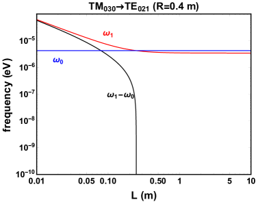
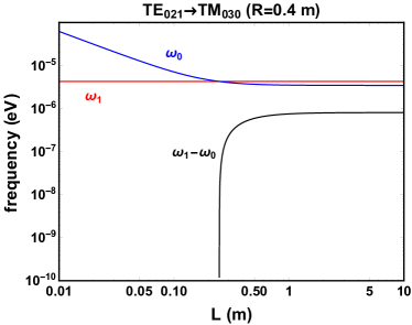
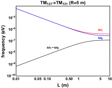
Figure 1: The frequencies $\omega_{1}$ (red), $\omega_{0}$ (blue) and $\omega_{1}-\omega_{0}$ (black) versus the height of cylinder for ${\rm TM}_{030}\to{\rm TE}_{021}$ and ${\rm TE}_{021}\to{\rm TM}_{030}$ transitions (top), and ${\rm TM}_{121}\to{\rm TM}_{131}$ transition (bottom).

The total noise becomes

$$S_{\rm noise}(\omega)=S_{\rm ql}(\omega)+\frac{Q_{1}}{Q_{\rm cpl}}(S_{\rm th}(\omega)+S_{\rm phase}(\omega)+S^{(1)}_{\rm mech}(\omega))+\frac{Q_{0}}{Q_{\rm cpl}}S^{(0)}_{\rm mech}(\omega)\;,$$ (88)

where an additional factor ${Q_{1}}/{Q_{\rm cpl}}$ is introduced to describe the signal power transmitted from cavity to readout waveguide. The last term describes the mechanical noise from pump mode with frequency $\omega_{0}$. One adds a pre-factor ${Q_{0}}/{Q_{\rm cpl}}$ to describe the coupling between readout and pump mode. The amplifier noise is intrinsic noise of amplifier and thus there is no fraction in front of it. Then, the signal-to-noise ratio (SNR) is given by

$$({\rm SNR})^{2}\simeq t_{\rm int}\int^{\infty}_{0}d\omega\Big{(}\frac{S_{\rm sig}(\omega)}{S_{\rm noise}(\omega)}\Big{)}^{2}\;,$$ (89)

where $t_{\rm int}\simeq t_{e}~{}{\Delta\omega_{sc}}/{m_{a}}$ with an e-fold time $t_{e}=10^{7}~{}s$ and $\Delta\omega_{sc}\simeq{\rm max}(m_{a}/Q_{a},\omega_{1}/Q_{1})$ being single scan width. Considering that the signal power from cavity needs to be received by the readout waveguide, in the above SNR formula, the PSD of signal is also modified as follows

$$S_{\rm sig}(\omega)\rightarrow\frac{Q_{1}}{Q_{\rm cpl}}S_{\rm sig}(\omega)\;.$$ (90)

We require ${\rm SNR}>1$ to show the sensitivity of the two-mode SRF cavity to the generic axion couplings. For $g_{a\gamma\gamma}$, $g_{aAA}$ and $g_{aBB}$ couplings, we assume the cavity column as $V=1~{}{\rm m}^{3}$ and the factor of $\eta\simeq 1$. For $g_{a\gamma\gamma}^{\cancel{\rm CP}}$ and $g_{aAB}$, we instead fix $R\approx 5$ m and vary the length $L$ from 0.01 m to 10 m.

In Figs. 2 and 3, we show the expected sensitivity bounds on generic ULDM couplings. The bounds on conventional coupling $g_{a\gamma\gamma}$ and $g_{aAA}$ restore the result in Ref. Berlin et al. (2020) with $Q_{\rm int}=10^{12}$. For $g_{aBB}$ coupling, we take a conservative magnitude of electric field $E_{0}=50~{}{\rm V/m}$. The axion mass lower than $10^{-6}$ eV can be probed by the axion-induced frequency conversion in SRF cavity with electric field. For $g_{a\gamma\gamma}^{\cancel{\rm CP}}$ and $g_{aAB}$ couplings, as discussed above, the reachable range of axion mass $10^{-9}\sim 10^{-7}$ eV is determined by the scope of adjusted cavity height $L$. To probe $g_{aAB}$ coupling, one needs $E_{0}\simeq 100~{}{\rm kV/m}$ which is lower than the breakdown electric field strength of a normal capacitor Chen et al. (2020); Zouache and Lefort (1997).

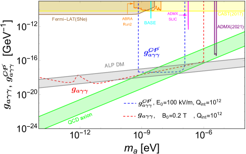
Figure 2: The expected sensitivity bounds of $g_{a\gamma\gamma}$ with $B_{0}=0.2~{}{\rm T}$ (red dashed line) and $g_{a\gamma\gamma}^{\cancel{\rm CP}}$ with $E_{0}=100~{}{\rm kV/m}$ (blue dashed line) as a function of $m_{a}$. The theoretical predictions of $g_{a\gamma\gamma}$ from QCD axion (green region) Di Luzio et al. (2020) and ALP DM for the standard cosmology with the initial misalignment angle of $\theta_{0}\in[0.1,1]$ (gray region) Blinov et al. (2019) are also presented. Some existing or potential exclusion limits on conventional coupling $g_{a\gamma\gamma}$ are shown for reference, including ABRACADABRA Run 2 (orange) Salemi et al. (2021), CAST (yellow) Anastassopoulos et al. (2017), ADMX 2021 (purple) Bartram et al. (2021), ADMX SLIC (magenta) Crisosto et al. (2020), BASE (cyan) Devlin et al. (2021), Fermi-LAT (brown) Meyer and Petrushevska (2020).

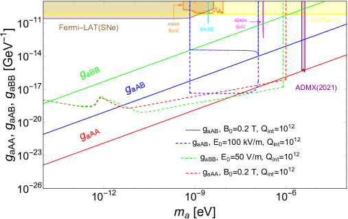
Figure 3: The expected sensitivity bounds of $g_{aAA}$ with $B_{0}=0.2~{}{\rm T}$ (red dashed line), $g_{aAB}$ with $B_{0}=0.2~{}{\rm T}$ (blue dotted line) and $E_{0}=100~{}{\rm kV/m}$ (blue dashed line) and $g_{aBB}$ with $E_{0}=50~{}{\rm kV/m}$ (green dashed line). The theoretical predictions of $g_{aAA}$, $g_{aAB}$ and $g_{aBB}$ (solid) Sokolov and Ringwald (2022) are also presented. Some existing or potential exclusion limits on conventional coupling $g_{a\gamma\gamma}$ are shown for reference, including ABRACADABRA Run 2 (orange) Salemi et al. (2021), CAST (yellow) Anastassopoulos et al. (2017), ADMX 2021 (purple) Bartram et al. (2021), ADMX SLIC (magenta) Crisosto et al. (2020), BASE (cyan) Devlin et al. (2021), Fermi-LAT (brown) Meyer and Petrushevska (2020).

V Conclusion

The ULDM such as axion or wavelike scalar is a plausible DM candidate. The possible non-standard ULDM couplings, for instance CP violating coupling, recently draw much attention. In this work we investigate the detection of non-standard electromagnetic couplings in a few benchmark models of ULDM. For illustration, we consider the generic axion electrodynamics as well as the newly proposed axion electromagnetodynamics based on the QEMD framework.

The SRF cavity with two-mode has more advantages than the traditional cavity approach with static background field or the LC circuit regime. It prefers a high quality factor and is sensitive to much lighter axion. We utilize the two-mode SRF cavity to probe the non-standard couplings of ULDM with frequency lower than GHz. We find that one can impose oscillating magnetic field and electric field to detect ordinary axion coupling $g_{a\gamma\gamma}$ and CP violating coupling $g_{a\gamma\gamma}^{\cancel{\rm CP}}$, respectively. In the QEMD axion framework, the background magnetic (electric) field can be introduced to probe both $g_{aAA}$ ($g_{aBB}$) and $g_{aAB}$ couplings. The choices of the transverse electromagnetic modes and the index integers are limited by the corresponding selection rules. Finally, we show the sensitivity of the two-mode SRF cavity to the above non-standard axion couplings.

Appendix A The QEMD axion theory

The equal-time canonical commutation relations between the two potentials in QEMD were established as Zwanziger (1971)

$$[A^{\mu}(t,\vec{x}),B^{\nu}(t,\vec{y})] = i\epsilon^{\mu\nu}_{~{}~{}\kappa 0}n^{\kappa}(n\cdot\partial)^{-1}(\vec{x}-\vec{y})\;,$$ (91)

$$~{}[A^{\mu}(t,\vec{x}),A^{\nu}(t,\vec{y})] = [B^{\mu}(t,\vec{x}),B^{\nu}(t,\vec{y})]=-i(g_{0}^{~{}\mu}n^{\nu}+g_{0}^{~{}\nu}n^{\mu})(n\cdot\partial)^{-1}(\vec{x}-\vec{y})\;.$$ (92)

The electromagnetic field strength tensors $F$ and $F^{d}$ in Eq. (13) satisfy

$$n\cdot F=n\cdot(\partial\wedge A)\;,~{}~{}n\cdot F^{d}=n\cdot(\partial\wedge B)\;.$$ (93)

The two four-potentials have opposite parities. In the absence of electric and magnetic currents $J_{e},J_{m}$, they have a simplified form as

$$F=\partial\wedge A=-(\partial\wedge B)^{d}\;,~{}~{}~{}F^{d}=\partial\wedge B=(\partial\wedge A)^{d}\;.$$ (94)

The Lagrangian for the anomalous interactions of axion based on QEMD is given by Sokolov and Ringwald (2022)

$$\mathcal{L} \supset -{1\over 4}g_{aAA}~{}a~{}{\rm tr}[(\partial\wedge A)(\partial\wedge A)^{d}]-{1\over 4}g_{aBB}~{}a~{}{\rm tr}[(\partial\wedge B)(\partial\wedge B)^{d}]$$ (95)

$$-{1\over 2}g_{aAB}~{}a~{}{\rm tr}[(\partial\wedge A)(\partial\wedge B)^{d}]\;.$$

The first two operators are CP-conserving axion interactions. The relevant couplings $g_{aAA}$ and $g_{aBB}$ are governed by the $U(1)_{\rm PQ}U(1)_{\rm E}^{2}$ and $U(1)_{\rm PQ}U(1)_{\rm M}^{2}$ anomalies, respectively. As $A^{\mu}$ and $B^{\mu}$ have opposite parities, the third operator is a CP-violating one and its coupling $g_{aAB}$ is given by the $U(1)_{\rm PQ}U(1)_{\rm E}U(1)_{\rm M}$ anomaly. The inclusion of this term accounts for the intrinsic CP violation in a dyon theory. In terms of classical electromagnetic fields, the above Lagrangian becomes

$$\mathcal{L} \supset -{1\over 4}(g_{aAA}-g_{aBB})~{}a~{}F_{\mu\nu}F^{d~{}\mu\nu}+{1\over 2}g_{aAB}~{}a~{}F_{\mu\nu}F^{\mu\nu}$$ (96)

$$= (g_{aAA}-g_{aBB})~{}a~{}\vec{\mathbb{B}}\cdot\vec{\mathbb{E}}+g_{aAB}~{}a~{}(\vec{\mathbb{B}}^{2}-\vec{\mathbb{E}}^{2})\;.$$

Note that the QEMD theory has an intrinsic source of CP violation. It is because the spectrum of dyon charges is not CP invariant with only a state $(q,g)$ and without its CP conjugate state $(-q,g)$. The intrinsic CP violation of high energy QEMD is transferred to the low-energy axion-photon EFT after integrating out heavy fermionic dyons with charges $(q,g)$. The coefficient $g_{aAB}$ is determined by the CP violating anomaly coefficient and the $g_{aAB}$ term in the Lagrangian is a CP-odd term. They reflect the intrinsic CP violation of QEMD.

One can propose a KSVZ-like theory with heavy PQ-charged fermions $\psi$ as a UV completion Sokolov and Ringwald (2022). The Lagrangian for the fermions $\psi$ is

$$\mathcal{L}\supset i\bar{\psi}\gamma^{\mu}D_{\mu}\psi+y\Phi\bar{\psi}_{L}\psi_{R}+h.c.\;,$$ (97)

where $D_{\mu}=\partial_{\mu}-eq_{\psi}A_{\mu}-g_{0}g_{\psi}B_{\mu}$ is a covariant derivative with both $A_{\mu}$ and $B_{\mu}$ four-potentials multiplied by the corresponding electric and magnetic charges, $e$ is the unit of electric charge, $g_{0}$ is the minimal magnetic charge with $g_{0}=2\pi/e$ in the Dirac-Schwinger-Zwanziger (DSZ) quantization condition, and $\Phi$ is the PQ complex scalar field. One can then calculate the coupling coefficients as

$$g_{aAA}={Ee^{2}\over 4\pi^{2}v_{\rm PQ}}\;,~{}~{}g_{aBB}={Mg_{0}^{2}\over 4\pi^{2}v_{\rm PQ}}\;,~{}~{}g_{aAB}={Deg_{0}\over 4\pi^{2}v_{\rm PQ}}\;,$$ (98)

where $v_{\rm PQ}$ is the $U(1)_{\rm PQ}$ symmetry breaking scale. $E(M)$ is the electric (magnetic) anomaly coefficient and $D$ is the mixed electric-magnetic CP-violating anomaly coefficient. They are obtained by integrating out PQ-charged fermions $\psi$ with electric and magnetic charges. Ref. Sokolov and Ringwald (2022) demonstrated the calculation of the anomaly coefficients by following Fujikawa’s path integral method Fujikawa (1979). As the DSZ quantization condition indicates $g_{0}\gg e$, we have the scaling of the axion-photon couplings as $g_{aBB}\gg|g_{aAB}|\gg g_{aAA}$.

Appendix B The PSD derivation

We can rewrite the $e_{1}(\omega)$ in $\langle e_{1}(\omega)e_{1}^{*}(\omega^{\prime})\rangle$ as

$$e_{1}(\omega) = g_{a\gamma\gamma}\frac{-\omega}{k_{1}(\omega)}\int{d\omega^{\prime}\over 2\pi}(\omega-\omega^{\prime})b_{0}(\omega^{\prime})a(\omega-\omega^{\prime})\frac{\int_{V}\tilde{\vec{\mathbb{E}}}_{1}^{*}\cdot\tilde{\vec{\mathbb{B}}}_{0}}{\int_{V}\left|\tilde{\vec{\mathbb{E}}}_{1}(\vec{r})\right|^{2}}$$ (99)

$$= \beta B(\omega)(\frac{1}{i})[b_{0}(\omega)\otimes(i\omega a(\omega))]$$

$$= \beta B(\omega)(-i)A(\omega)\;,$$

where $\beta=\frac{1}{2\pi}g_{a\gamma\gamma}\frac{\int_{V}\tilde{\vec{\mathbb{E}}}_{1}^{\ast}\cdot\tilde{\vec{\mathbb{B}}}_{0}}{\int_{V}\left|\tilde{\vec{\mathbb{E}}}_{1}(\vec{r})\right|^{2}}$, $B(\omega)=\frac{-\omega}{k_{1}(\omega)}$, and $A(\omega)=b_{0}(\omega)\otimes(i\omega a(\omega))$ with $\otimes$ denoting the convolution. Then, we have

$$\langle e_{1}(\omega)e_{1}^{*}(\omega^{\prime})\rangle =\beta^{2}\langle B(\omega)B^{\ast}(\omega^{\prime})A(\omega)A^{\ast}(\omega^{\prime})\rangle$$ (100)

$$=\beta^{2}\langle B(\omega)B^{\ast}(\omega^{\prime})\rangle~{}\langle A(\omega)A^{\ast}(\omega^{\prime})\rangle$$ (101)

$$=\beta^{2}B(\omega)B^{\ast}(\omega^{\prime})~{}\langle A(\omega)A^{\ast}(\omega^{\prime})\rangle$$ (102)

$$=\beta^{2}B(\omega)B^{\ast}(\omega^{\prime})~{}S_{A}(\omega)\delta(\omega-\omega^{\prime})\;,$$ (103)

where in the second step we use the statistical independence of two independent functions $A(\omega)$ and $B(\omega)$. Thus, the time expectation of their product can be written as the product of their time expectations. The last step uses the relation in Eq. (27). According to Eq. (30), we obtain

$$S_{\rm sig}(\omega)=\alpha\beta^{2}|B(\omega)|^{2}S_{A}(\omega)\;,$$ (104)

where $\alpha={\omega_{1}\over Q_{1}}\int_{V}\left|\tilde{\vec{\mathbb{E}}}_{1}(\vec{r})\right|^{2}$. Using convolution theorem, one also gets the Fourier transform of $A(\omega)$

$$A(t)=\frac{1}{2\pi}\int d\omega~{}e^{i\omega t}A(\omega)=b_{0}(t)\partial_{t}a(t)\;.$$ (105)

Then, we need to obtain $S_{A}(\omega)$ which is the PSD of two functions’ product $A(t)$.

Firstly, one can define an auto-correlation function as follows

$$R_{f}(\tau)=\langle f(t)f(t+\tau)\rangle\;,~{}~{}R_{f}(0)=\langle f(t)^{2}\rangle\;.$$ (106)

One can obtain the PSD as the Fourier transform of function $R_{f}(\tau)$

$$S_{f}(\omega) =\int d\tau~{}e^{-i\omega\tau}R_{f}(\tau)\;,~{}~{}R_{f}(\tau)={\frac{1}{2\pi}}\int d\omega~{}e^{i\omega\tau}S_{f}(\omega)\;.$$ (107)

If $x(t)$ and $y(t)$ are two statistically independent functions. Their auto-correlation functions are $R_{x}(\tau)$ and $R_{y}(\tau)$, respectively. Now we define $z(t)=x(t)y(t)$. Then, the auto-correlation function of it can be obtained as

$$R_{z}(\tau)= \langle z(t)z(t+\tau)\rangle$$

$$= \langle x(t)y(t)~{}x(t+\tau)y(t+\tau)\rangle$$

$$= \langle x(t)x(t+\tau)\rangle~{}\langle y(t)y(t+\tau)\rangle$$

$$= R_{x}(\tau)R_{y}(\tau)\;.$$ (108)

From the Wiener-Khinchin theorem, we get

$$S_{z}(\omega) =\int d\tau~{}e^{-i\omega\tau}R_{z}=\int d\tau~{}e^{-i\omega\tau}R_{x}(\tau)R_{y}(\tau)$$

$$=S_{x}(\omega)\otimes S_{y}(\omega)\;.$$ (109)

By identifying $R_{A}(\tau)=\langle A(t)A(t+\tau)\rangle$, the PSD of $A(t)$ becomes

$$S_{A}(\omega) = \int d\tau e^{-i\omega\tau}R_{A}(\tau)$$ (110)

$$= \int d\tau e^{-i\omega\tau}R_{b_{0}}(\tau)R_{\partial_{t}a}(\tau)$$

$$= S_{b_{0}}(\omega)\otimes S_{\partial_{t}a}(\omega)\;.$$

Given this result, the PSD of our signal is given by

$$S_{\rm sig}(\omega)=\alpha\beta^{2}|B(\omega)|^{2}S_{b_{0}}(\omega)\otimes S_{\partial_{t}a}(\omega)\;.$$ (111)

Next, we should express $S_{\partial_{t}a}(\omega)$. We find

$$\omega^{2}S_{a}(\omega)= \int d\tau~{}e^{-i\omega\tau}\omega^{2}R_{a}(\tau)$$

$$= \int d\tau~{}e^{-i\omega\tau}\omega^{2}\langle a(t)a(t+\tau)\rangle$$

$$= \int d\tau~{}e^{-i\omega\tau}\langle(i\omega)a(t)~{}~{}(-i\omega)a(t+\tau)\rangle$$

$$= \int d\tau~{}e^{-i\omega\tau}[\lim_{T\rightarrow\infty}\frac{1}{T}\int^{T/2}_{-T/2}dt~{}(i\omega)a(t)~{}~{}(-i\omega)a(t+\tau)]$$

$$= \int d\tau~{}e^{-i\omega\tau}[\lim_{T\rightarrow\infty}\frac{1}{T}\int^{T/2}_{-T/2}dt~{}(i\omega e^{i\omega t})a(t)~{}~{}(-i\omega e^{-i\omega t})a(t+\tau)]$$

$$= \int d\tau~{}e^{-i\omega\tau}[\lim_{T\rightarrow\infty}\frac{1}{T}\int^{T/2}_{-T/2}dt~{}\frac{\partial e^{i\omega t}}{\partial t}a(t)~{}~{}\frac{\partial e^{-i\omega t}}{\partial t}a(t+\tau)]$$ (112)

where $\langle\cdots\rangle$ is defined as $\lim_{T\rightarrow\infty}\frac{1}{T}\int^{T/2}_{-T/2}(\cdots)dt$. We integrate it by parts and get

$$\lim_{T\rightarrow\infty}\int^{T/2}_{-T/2}dt~{}\frac{\partial e^{i\omega t}}{\partial t}a(t)~{}~{}\frac{\partial e^{-i\omega t}}{\partial t}a(t+\tau)$$

$$= \lim_{T\rightarrow\infty}\int^{T/2}_{-T/2}dt~{}[\frac{d(e^{i\omega t}a(t))}{dt}-e^{i\omega t}\partial_{t}a(t)]~{}[\frac{d(e^{-i\omega t}a(t))}{dt}-e^{-i\omega t}\partial_{t}a(t+\tau)]$$

$$= \lim_{T\rightarrow\infty}\int^{T/2}_{-T/2}dt~{}[-e^{i\omega t}\partial_{t}a(t)][-e^{-i\omega t}\partial_{t}a(t+\tau)]$$

$$= \lim_{T\rightarrow\infty}\int^{T/2}_{-T/2}dt~{}\partial_{t}a(t)\partial_{t}a(t+\tau)\;.$$ (113)

Thus, we can get $S_{\partial_{t}a}(\omega)$ as follows

$$\omega^{2}S_{a}(\omega) =\int d\tau~{}e^{-i\omega\tau}[\lim_{T\rightarrow\infty}\int^{T/2}_{-T/2}dt~{}\partial_{t}a(t)\partial_{t}a(t+\tau)]$$

$$=S_{\partial_{t}a}(\omega)\;.$$ (114)

Finally, we obtain the PSD as

$$S_{\rm sig}(\omega) =\alpha\beta^{2}|B(\omega)|^{2}S_{b_{0}}(\omega)\otimes[\omega^{2}S_{a}(\omega)]$$

$$=\frac{\omega_{1}}{Q_{1}}g_{a\gamma\gamma}^{2}\frac{|\int_{V}\tilde{\vec{\mathbb{E}}}_{1}^{*}\cdot\tilde{\vec{\mathbb{B}}}_{0}|^{2}}{\int_{V}\left|\tilde{\vec{\mathbb{E}}}_{1}(\vec{r})\right|^{2}}\frac{\omega^{2}}{(\omega^{2}-\omega_{1}^{2})^{2}+(\omega\omega_{1}/Q_{1})^{2}}\int\frac{d\omega^{\prime}}{(2\pi)^{2}}S_{b_{0}}(\omega^{\prime})~{}(\omega^{\prime}-\omega)^{2}S_{a}(\omega^{\prime}-\omega)\;.$$ (115)

Appendix C The selection rules of $p$ integer in ${\rm TM}_{mnp}$ or ${\rm TE}_{mnp}$

We show the integral over the height coordinate $z$ relevant for the selection of $p$ integer.

The selection rule for $\int_{V}\vec{\mathbb{B}}\cdot\vec{\mathbb{B}}$ :

$$\int_{V}\vec{\mathbb{B}}^{\rm TE}_{1}\cdot\vec{\mathbb{B}}^{\rm TM}_{0}=\int_{V}\vec{\mathbb{B}}^{\rm TE}_{0}\cdot\vec{\mathbb{B}}^{\rm TM}_{1}\propto\int_{0}^{L}\cos(\frac{p_{0}\pi z}{L})\cos(\frac{p_{1}\pi z}{L})dz=\begin{cases}0&p_{1}\neq p_{0}\;,\\ \frac{L}{2}&p_{1}=p_{0}\;.\end{cases}$$ (116)

$$\int_{V}\vec{\mathbb{B}}^{\rm TM}_{1}\cdot\vec{\mathbb{B}}^{\rm TM}_{0}=\int_{V}\vec{\mathbb{B}}^{\rm TM}_{0}\cdot\vec{\mathbb{B}}^{\rm TM}_{1}\propto\int_{0}^{L}\cos(\frac{p_{0}\pi z}{L})\cos(\frac{p_{1}\pi z}{L})dz=\begin{cases}0&p_{1}\neq p_{0}\;,\\ \frac{L}{2}&p_{1}=p_{0}\;.\end{cases}$$ (117)

$$\int_{V}\vec{\mathbb{B}}^{\rm TE}_{1}\cdot\vec{\mathbb{B}}^{\rm TE}_{0}=\int_{V}\vec{\mathbb{B}}^{\rm TE}_{0}\cdot\vec{\mathbb{B}}^{\rm TE}_{1} \propto k_{1}\int_{0}^{L}\cos(\frac{p_{0}\pi z}{L})\cos(\frac{p_{1}\pi z}{L})dz+k_{2}\int_{0}^{L}\sin(\frac{p_{0}\pi z}{L})\sin(\frac{p_{1}\pi z}{L})dz$$ (118)

$$= \begin{cases}0&p_{1}\neq p_{0}\;,\\ \frac{L}{2}(k_{1}+k_{2})&p_{1}=p_{0}\;.\end{cases}$$

The selection rule for $\int_{V}\vec{\mathbb{E}}\cdot\vec{\mathbb{E}}$ :

$$\int_{V}\vec{\mathbb{E}}^{\rm TE}_{1}\cdot\vec{\mathbb{E}}^{\rm TM}_{0}=\int_{V}\vec{\mathbb{E}}^{\rm TE}_{0}\cdot\vec{\mathbb{E}}^{\rm TM}_{1}\propto\int_{0}^{L}\sin(\frac{p_{0}\pi z}{L})\sin(\frac{p_{1}\pi z}{L})dz=\begin{cases}0&p_{1}\neq p_{0}\;,\\ \frac{L}{2}&p_{1}=p_{0}\;.\end{cases}$$ (119)

$$\int_{V}\vec{\mathbb{E}}^{\rm TE}_{1}\cdot\vec{\mathbb{E}}^{\rm TE}_{0}=\int_{V}\vec{\mathbb{E}}^{\rm TE}_{0}\cdot\vec{\mathbb{E}}^{\rm TE}_{1}\propto\int_{0}^{L}\sin(\frac{p_{0}\pi z}{L})\sin(\frac{p_{1}\pi z}{L})dz=\begin{cases}0&p_{1}\neq p_{0}\;,\\ \frac{L}{2}&p_{1}=p_{0}\;.\end{cases}$$ (120)

$$\int_{V}\vec{\mathbb{E}}^{\rm TM}_{1}\cdot\vec{\mathbb{E}}^{\rm TM}_{0}=\int_{V}\vec{\mathbb{E}}^{\rm TM}_{0}\cdot\vec{\mathbb{E}}^{\rm TM}_{1} \propto k_{1}\int_{0}^{L}\sin(\frac{p_{0}\pi z}{L})\sin(\frac{p_{1}\pi z}{L})dz+k_{2}\int_{0}^{L}\cos(\frac{p_{0}\pi z}{L})\cos(\frac{p_{1}\pi z}{L})dz$$ (121)

$$= \begin{cases}0&p_{1}\neq p_{0}\;,\\ \frac{L}{2}(k_{1}+k_{2})&p_{1}=p_{0}\;.\end{cases}$$

The selection rule for $\int_{V}\vec{\mathbb{B}}\cdot\vec{\mathbb{E}}$ :

$$\int_{V}\vec{\mathbb{B}}_{0}^{\rm TE}\cdot\vec{\mathbb{E}}_{1}^{\rm TE} \propto \int_{0}^{L}\cos(\frac{p_{0}\pi z}{L})\sin(\frac{p_{1}\pi z}{L})dz$$ (122)

$$= \frac{Lp_{1}}{\pi(p_{1}^{2}-p_{0}^{2})}\times\begin{cases}2&p_{1}+p_{0}\quad odd\;,\\ 0&p_{1}+p_{0}\quad even\;.\end{cases}$$

$$\int_{V}\vec{\mathbb{B}}_{1}^{\rm TE}\cdot\vec{\mathbb{E}}_{0}^{\rm TE} \propto \int_{0}^{L}\cos(\frac{p_{1}\pi z}{L})\sin(\frac{p_{0}\pi z}{L})dz$$ (123)

$$= \frac{Lp_{0}}{\pi(p_{0}^{2}-p_{1}^{2})}\times\begin{cases}2&p_{1}+p_{0}\quad odd\;,\\ 0&p_{1}+p_{0}\quad even\;.\end{cases}$$

$$\int_{V}\vec{\mathbb{B}}_{0}^{\rm TM}\cdot\vec{\mathbb{E}}_{1}^{\rm TM} \propto \int_{0}^{L}\cos(\frac{p_{0}\pi z}{L})\sin(\frac{p_{1}\pi z}{L})dz$$ (124)

$$= \frac{Lp_{1}}{\pi(p_{1}^{2}-p_{0}^{2})}\times\begin{cases}2&p_{1}+p_{0}\quad odd\;,\\ 0&p_{1}+p_{0}\quad even\;.\end{cases}$$

$$\int_{V}\vec{\mathbb{B}}_{1}^{\rm TM}\cdot\vec{\mathbb{E}}_{0}^{\rm TM} \propto \int_{0}^{L}\cos(\frac{p_{1}\pi z}{L})\sin(\frac{p_{0}\pi z}{L})dz$$ (125)

$$= \frac{Lp_{0}}{\pi(p_{0}^{2}-p_{1}^{2})}\times\begin{cases}2&p_{1}+p_{0}\quad odd\;,\\ 0&p_{1}+p_{0}\quad even\;.\end{cases}$$

$$\int_{V}\vec{\mathbb{B}}_{0}^{\rm TM}\cdot\vec{\mathbb{E}}_{1}^{\rm TE}\propto\int_{0}^{L}\cos(\frac{p_{0}\pi z}{L})\sin(\frac{p_{1}\pi z}{L})dz=\frac{Lp_{1}}{\pi(p_{1}^{2}-p_{0}^{2})}\times\begin{cases}2&p_{1}+p_{0}\quad odd\;,\\ 0&p_{1}+p_{0}\quad even\;.\end{cases}$$ (126)

$$\int_{V}\vec{\mathbb{B}}_{1}^{\rm TM}\cdot\vec{\mathbb{E}}_{0}^{\rm TE}\propto\int_{0}^{L}\cos(\frac{p_{1}\pi z}{L})\sin(\frac{p_{0}\pi z}{L})dz=\frac{Lp_{0}}{\pi(p_{0}^{2}-p_{1}^{2})}\times\begin{cases}2&p_{1}+p_{0}\quad odd\;,\\ 0&p_{1}+p_{0}\quad even\;.\end{cases}$$ (127)

$$\int_{V}\vec{\mathbb{B}}_{0}^{\rm TE}\cdot\vec{\mathbb{E}}_{1}^{\rm TM} \propto k_{1}\int_{0}^{L}\cos(\frac{p_{0}\pi z}{L})\sin(\frac{p_{1}\pi z}{L})dz+k_{2}\int_{0}^{L}\sin(\frac{p_{0}\pi z}{L})\cos(\frac{p_{1}\pi z}{L})dz$$ (128)

$$= \frac{L(k_{1}~{}p_{1}+k_{2}~{}p_{0})}{\pi(p_{1}^{2}-p_{0}^{2})}\times\begin{cases}2&p_{1}+p_{0}\quad odd\;,\\ 0&p_{1}+p_{0}\quad even\;.\end{cases}$$

$$\int_{V}\vec{\mathbb{B}}_{1}^{\rm TE}\cdot\vec{\mathbb{E}}_{0}^{\rm TM} \propto k_{1}\int_{0}^{L}\cos(\frac{p_{1}\pi z}{L})\sin(\frac{p_{0}\pi z}{L})dz+k_{2}\int_{0}^{L}\sin(\frac{p_{1}\pi z}{L})\cos(\frac{p_{0}\pi z}{L})dz$$ (129)

$$= \frac{L(k_{1}~{}p_{0}+k_{2}~{}p_{1})}{\pi(p_{0}^{2}-p_{1}^{2})}\times\begin{cases}2&p_{1}+p_{0}\quad odd\;,\\ 0&p_{1}+p_{0}\quad even\;.\end{cases}$$

References

- Peccei and Quinn (1977a) R. D. Peccei and H. R. Quinn, Phys. Rev. Lett. 38, 1440 (1977a).
- Peccei and Quinn (1977b) R. D. Peccei and H. R. Quinn, Phys. Rev. D 16, 1791 (1977b).
- Weinberg (1978) S. Weinberg, Phys. Rev. Lett. 40, 223 (1978).
- Wilczek (1978) F. Wilczek, Phys. Rev. Lett. 40, 279 (1978).
- Baluni (1979) V. Baluni, Phys. Rev. D 19, 2227 (1979).
- Crewther et al. (1979) R. J. Crewther, P. Di Vecchia, G. Veneziano, and E. Witten, Phys. Lett. B 88, 123 (1979), [Erratum: Phys.Lett.B 91, 487 (1980)].
- Kim (1979) J. E. Kim, Phys. Rev. Lett. 43, 103 (1979).
- Shifman et al. (1980) M. A. Shifman, A. I. Vainshtein, and V. I. Zakharov, Nucl. Phys. B 166, 493 (1980).
- Dine et al. (1981) M. Dine, W. Fischler, and M. Srednicki, Phys. Lett. B 104, 199 (1981).
- Zhitnitsky (1980) A. R. Zhitnitsky, Sov. J. Nucl. Phys. 31, 260 (1980).
- Baker et al. (2006) C. A. Baker et al., Phys. Rev. Lett. 97, 131801 (2006), arXiv:hep-ex/0602020 .
- Pendlebury et al. (2015) J. M. Pendlebury et al., Phys. Rev. D 92, 092003 (2015), arXiv:1509.04411 [hep-ex] .
- Preskill et al. (1983) J. Preskill, M. B. Wise, and F. Wilczek, Phys. Lett. B 120, 127 (1983).
- Dine and Fischler (1983) M. Dine and W. Fischler, Phys. Lett. B 120, 137 (1983).
- Di Luzio et al. (2020) L. Di Luzio, M. Giannotti, E. Nardi, and L. Visinelli, Phys. Rept. 870, 1 (2020), arXiv:2003.01100 [hep-ph] .
- Sikivie (2021) P. Sikivie, Reviews of Modern Physics 93 (2021), 10.1103/revmodphys.93.015004.
- Di Luzio et al. (2023) L. Di Luzio, G. Levati, and P. Paradisi, (2023), arXiv:2311.12158 [hep-ph] .
- Luo and Mathur (2023) X. Luo and A. Mathur, (2023), arXiv:2311.03536 [hep-ph] .
- Anzuini et al. (2023) F. Anzuini, A. Gómez-Bañón, J. A. Pons, A. Melatos, and P. D. Lasky, (2023), arXiv:2311.13776 [hep-ph] .
- Witten (1979) E. Witten, Phys. Lett. B 86, 283 (1979).
- Fischler and Preskill (1983) W. Fischler and J. Preskill, Phys. Lett. B 125, 165 (1983).
- Sokolov and Ringwald (2022) A. V. Sokolov and A. Ringwald, (2022), arXiv:2205.02605 [hep-ph] .
- Sokolov and Ringwald (2023) A. V. Sokolov and A. Ringwald, Annalen Phys. 2023 (2023), 10.1002/andp.202300112, arXiv:2303.10170 [hep-ph] .
- Heidenreich et al. (2023) B. Heidenreich, J. McNamara, and M. Reece, (2023), arXiv:2309.07951 [hep-ph] .
- Li and Zhang (2023a) T. Li and R.-J. Zhang, (2023a), arXiv:2312.01355 [hep-ph] .
- Li et al. (2023a) T. Li, R.-J. Zhang, and C.-J. Dai, JHEP 03, 088 (2023a), arXiv:2211.06847 [hep-ph] .
- Tobar et al. (2022) M. E. Tobar, C. A. Thomson, B. T. McAllister, M. Goryachev, A. Sokolov, and A. Ringwald, Annalen Phys. 2023, 2200594 (2022), arXiv:2211.09637 [hep-ph] .
- McAllister et al. (2022) B. T. McAllister, A. Quiskamp, C. O’Hare, P. Altin, E. Ivanov, M. Goryachev, and M. Tobar, Annalen Phys. 2023, 2200622 (2022), arXiv:2212.01971 [hep-ph] .
- Li et al. (2023b) T. Li, C.-J. Dai, and R.-J. Zhang, (2023b), arXiv:2304.12525 [hep-ph] .
- Li and Zhang (2023b) T. Li and R.-J. Zhang, Chin. Phys. C 47, 123104 (2023b), arXiv:2305.01344 [hep-ph] .
- Tobar et al. (2023) M. E. Tobar, A. V. Sokolov, A. Ringwald, and M. Goryachev, Phys. Rev. D 108, 035024 (2023), arXiv:2306.13320 [hep-ph] .
- Patkos (2023) A. Patkos, Mod. Phys. Lett. A 38, 2350137 (2023), arXiv:2309.05523 [hep-ph] .
- Schwinger (1966) J. S. Schwinger, Phys. Rev. 144, 1087 (1966).
- Zwanziger (1968) D. Zwanziger, Phys. Rev. 176, 1489 (1968).
- Zwanziger (1971) D. Zwanziger, Phys. Rev. D 3, 880 (1971).
- Sikivie (1983) P. Sikivie, Phys. Rev. Lett. 51, 1415 (1983), [Erratum: Phys.Rev.Lett. 52, 695 (1984)].
- Berlin et al. (2020) A. Berlin, R. T. D’Agnolo, S. A. R. Ellis, C. Nantista, J. Neilson, P. Schuster, S. Tantawi, N. Toro, and K. Zhou, JHEP 07, 088 (2020), arXiv:1912.11048 [hep-ph] .
- Lasenby (2020) R. Lasenby, Phys. Rev. D 102, 015008 (2020), arXiv:1912.11056 [hep-ph] .
- Berlin et al. (2021) A. Berlin, R. T. D’Agnolo, S. A. R. Ellis, and K. Zhou, Phys. Rev. D 104, L111701 (2021), arXiv:2007.15656 [hep-ph] .
- Gao and Harnik (2021) C. Gao and R. Harnik, JHEP 07, 053 (2021), arXiv:2011.01350 [hep-ph] .
- Salnikov et al. (2021) D. Salnikov, P. Satunin, D. V. Kirpichnikov, and M. Fitkevich, JHEP 03, 143 (2021), arXiv:2011.12871 [hep-ph] .
- Berlin et al. (2022) A. Berlin et al., (2022), arXiv:2203.12714 [hep-ph] .
- Giaccone et al. (2022) B. Giaccone et al., (2022), arXiv:2207.11346 [hep-ex] .
- Romanenko et al. (2023) A. Romanenko et al., Phys. Rev. Lett. 130, 261801 (2023), arXiv:2301.11512 [hep-ex] .
- Tang et al. (2023) Z. Tang et al., (2023), arXiv:2305.09711 [hep-ex] .
- Workman and Others (2022) R. L. Workman and Others (Particle Data Group), PTEP 2022, 083C01 (2022).
- Ponce de Leon (2015) J. Ponce de Leon, European Journal of Physics 36 (2015), 10.1088/0143-0807/36/1/015016.
- Bernard et al. (2001) P. Bernard, G. Gemme, R. Parodi, and E. Picasso, Rev. Sci. Instrum. 72, 2428 (2001), arXiv:gr-qc/0103006 .
- Chen et al. (2020) W. Chen, Y. Gao, and Q. Yang, (2020), arXiv:2012.13946 [hep-ph] .
- Zouache and Lefort (1997) N. Zouache and A. Lefort, IEEE Transactions on Dielectrics and Electrical Insulation 4, 358 (1997).
- Blinov et al. (2019) N. Blinov, M. J. Dolan, P. Draper, and J. Kozaczuk, Phys. Rev. D 100, 015049 (2019), arXiv:1905.06952 [hep-ph] .
- Salemi et al. (2021) C. P. Salemi et al., Phys. Rev. Lett. 127, 081801 (2021), arXiv:2102.06722 [hep-ex] .
- Anastassopoulos et al. (2017) V. Anastassopoulos et al. (CAST), Nature Phys. 13, 584 (2017), arXiv:1705.02290 [hep-ex] .
- Bartram et al. (2021) C. Bartram et al. (ADMX), Phys. Rev. Lett. 127, 261803 (2021), arXiv:2110.06096 [hep-ex] .
- Crisosto et al. (2020) N. Crisosto, P. Sikivie, N. S. Sullivan, D. B. Tanner, J. Yang, and G. Rybka, Phys. Rev. Lett. 124, 241101 (2020), arXiv:1911.05772 [astro-ph.CO] .
- Devlin et al. (2021) J. A. Devlin et al., Phys. Rev. Lett. 126, 041301 (2021), arXiv:2101.11290 [astro-ph.CO] .
- Meyer and Petrushevska (2020) M. Meyer and T. Petrushevska, Phys. Rev. Lett. 124, 231101 (2020), [Erratum: Phys.Rev.Lett. 125, 119901 (2020)], arXiv:2006.06722 [astro-ph.HE] .
- Fujikawa (1979) K. Fujikawa, Phys. Rev. Lett. 42, 1195 (1979).