Graph-accelerated Markov Chain Monte Carlo
using Approximate Samples

Abstract

In recent years, it has become increasingly easy to obtain approximate posterior samples via efficient computation algorithms, such as those in variational Bayes. On the other hand, concerns exist on the accuracy of uncertainty estimates, which make it tempting to consider exploiting the approximate samples in canonical Markov chain Monte Carlo algorithms. A major technical barrier is that the approximate sample, when used as a proposal in Metropolis-Hastings steps, tends to have a low acceptance rate as the dimension increases. In this article, we propose a simple yet general solution named “graph-accelerated Markov Chain Monte Carlo”. We first build a graph with each node location assigned to an approximate sample, then we run Markov chain Monte Carlo with random walks over the graph. In the first stage, we optimize the choice of graph edges to enforce small differences in posterior density/probability between neighboring nodes, while encouraging edges to correspond to large distances in the parameter space. This optimized graph allows us to accelerate a canonical Markov transition kernel through mixing with a large-jump Metropolis-Hastings step, when collecting Markov chain samples at the second stage. Due to its simplicity, this acceleration can be applied to most of the existing Markov chain Monte Carlo algorithms. We theoretically quantify the rate of acceptance as dimension increases, and show the effects on improved mixing time. We demonstrate our approach through improved mixing performances for challenging sampling problems, such as those involving multiple modes, non-convex density contour, or large-dimension latent variables.
KEY WORDS: Conductance, Graph Bottleneck, Mixture Transition Kernel, Spanning Tree Graph, Latent Gaussian Model.

1 Introduction

Bayesian approaches are convenient for incorporating prior information, enabling model-based uncertainty quantification, and facilitating flexible model extension. Among the sampling algorithms for posterior computation, Markov chain Monte Carlo is arguably the most popular method and uses a Markov transition kernel (a conditional distribution given the current parameter value) to produce an update to the parameter. As one can flexibly choose transition kernel under a set of fairly straightforward principles, the algorithm can handle parameters in a multi-dimensional and complicated space, such as those involving latent variables (Tanner and Wong, 1987; Gelman, 2004), constraints (Gelfand et al., 1992; Duan et al., 2020; Presman and Xu, 2023), discrete or hierarchical structure (Chib and Carlin, 1999; Papaspiliopoulos et al., 2007); among many others. A major strength is that many Markov chain Monte Carlo algorithms have an exact convergence guarantee (Roberts and Rosenthal, 2004) — as the number of Markov chain iterations goes to infinity, the distribution of the Markov chain samples converge to the target posterior distribution. There is a rich literature on establishing such convergence guarantee for popular Markov chain Monte Carlo algorithms. The literature covers Gibbs sampling (Roberts and Polson, 1994; Gelfand, 2000), Metropolis–Hastings (Roberts and Smith, 1994; Jones et al., 2014), slice sampling (Roberts and Rosenthal, 1999; Neal, 2003; Natarovskii et al., 2021), hybrid Monte Carlo (Durmus et al., 2017; Durmus et al., 2020), and non-reversible extensions such as piecewise deterministic Markov process (Costa and Dufour, 2008; Fearnhead et al., 2018; Bierkens et al., 2019).

On the other hand, Markov chain Monte Carlo is not without its challenges, especially in advanced models that involve a high-dimensional parameter, latent correlation, or hierarchical structure. For example, there is recent literature characterizing the curse of dimensionality that leads to slow convergence of some routinely used Gibbs sampler (Johndrow et al., 2019), which has subsequently inspired a flourish of remedial algorithms (Johndrow et al., 2020; Vono et al., 2022). More broadly speaking, the computing inefficiency happens when the Markov transition kernel creates high auto-correlation along the chain — under such a scenario, the effective change of parameter becomes quite small over many iterations. Due to this “slow mixing” issue, practical issues arise in applications: the sampler may take a long time to move away from the start region (where the chain is initialized) into the high posterior density/probability region; it may have difficulty crossing low-probability region that divides multiple posterior modes; it may lack an efficient proposal distribution that could significantly change the parameter value, due to the dependence on a high-dimensional latent variable (Rue et al., 2009).

Conventionally, one often views optimization as a competitor to Markov chain Monte Carlo, and as a class of algorithms incompatible with Bayesian models. This belief has been rapidly changed by the recent study of diffusion-based methods. To give a few examples, it has been pointed out that the (unadjusted overdamped) Langevin diffusion algorithm is equivalent to a gradient descent algorithm adding a Gaussian random walk in each step (Roberts and Tweedie, 1996; Roberts and Rosenthal, 1998; Dalalyan, 2017); as a result, similar acceleration for gradient descent could be applied in the diffusion algorithm for posterior approximation (Ma et al., 2021). Mimicking second-order optimization such as Newton descent, one could obtain a rapid diffusion on the probability space using the Fisher information metric (Girolami and Calderhead, 2011).

In parallel to these developments, variational algorithms have become very popular. One uses optimization to minimize a statistical divergence between the posterior distribution and a prescribed variational distribution, from which one could draw independent samples as a posterior approximation. The choice of variational distribution spans from mean-field approximation (uncorrelated parameter elements) (Blei et al., 2017), variational boosting (mixture) (Miller et al., 2017; Campbell and Li, 2019), to normalizing flow neural networks (black-box non-linear transform) (Papamakarios et al., 2021). In particular, the normalizing flow neural networks have received considerable attention lately due to the high computing efficiency under modern computing platforms, and its high flexibility during density approximation (for continuous parameter). Successes of normalizing flow variational approaches have been reported for approximating many posterior distributions, such as those that are multi-modal or ill-conditioned in density contour (Hoffman et al., 2018), as mentioned above. On the other hand, concerns exist about the accuracy of uncertainty estimates. In particular, the prescribed variational distribution may not be adequately flexible to approximate the target posterior. For example, the mean-field variational methods lead to a wrong estimate of posterior covariance, which has motivated the development of alternative variational distributions (Giordano et al., 2018). For neural network-based approximation, although positive result has been obtained for approximating the class of sub-Gaussian and log-Lipschitz posterior densities via a feed-forward neural network (Lu and Lu, 2020), for normalizing flow (as a neural network restricted for one-to-one mapping), severe limitations have been discovered even for approximating some simple distributions (Dupont et al., 2019; Kong and Chaudhuri, 2020). Practically, another concern is in the lack of diagnostic measures on the accuracy of approximation — since the target posterior density/probability often contains intractable normalizing constant, usually we do not know how close the minimized statistical divergence is to zero.

Naturally, it is tempting to consider combining strengths from both approximation methods and the canonical Markov chain Monte Carlo framework. One intuitive idea is to adopt the approximate samples to build a proposal distribution and accept or reject each drawn proposal via a Metropolis-Hastings adjustment step. Nevertheless, a technical barrier is the acceptance rate often rapidly decays to zero, as the parameter (and latent variable) dimension grows, which has inspired several solutions. One remedy is to divide the proposal into several blocks (each in low dimension), then accept or reject the change in each block sequentially via a Metropolis-within-Gibbs sampler, which unfortunately often leads to slow mixing. Another idea is to use each approximate sample as an initial state and run multiple parallel Markov chains (Hoffman et al., 2018). Lastly, a recently popularized solution is to combine approximate samples with a Metropolis-adjusted diffusion algorithm such as Hamiltonian Monte Carlo (Betancourt et al., 2017). For example, Gabrié et al. (2022) interleave two Metropolis-Hastings steps, one using Langevin/Hamiltonian diffusion and one using independent proposal from an approximate sampler (normalizing flow); Toth et al. (2020) approximate the diffusion by training the gradients of a neural network to match the time derivative of the Hamiltonian, gaining higher efficiency than a differential equation integrator. For a recent review on this topic, see Winter et al., 2023 (arXiv:2304.11251). In addition, there are a few new adaptive Markov chain Monte Carlo algorithms for multi-modal posterior estimation (Pompe et al., 2020; Yi et al., 2023), based on interleaving the mode estimation steps and proposal moves between modes.

Despite similar motivation, our goal is to build a simple and general Markov chain Monte Carlo algorithm for which one could exploit an approximate sampler in an out-of-box manner without any need for customization. The chosen approximation method could be as advanced as a normalizing flow neural network, or as simple as an existing Markov chain Monte Carlo (which could suffer from slow mixing). Our main idea is to first collect approximate samples, build a graph to connect these samples and run the Markov chain Monte Carlo via a mixture transition kernel of a canonical baseline kernel and a graph jump step. We will demonstrate how this method leads to accelerated mixing of the Markov chains in both theory and applications.

2 Method

Let $\theta\in\Theta\subseteq\mathbb{R}^{p}$ be the parameter of interest and our goal is to draw samples from the posterior distribution $\Pi(\theta\mid y)\propto L(y;\theta)\Pi_{0}(\theta)$, with $L$ the likelihood and $\Pi_{0}$ the prior. To be general, this form also extends to the case of augmented likelihood containing latent variable $z$ in addition to the parameter of interest $\tilde{\theta}$, $\Pi\{(\tilde{\theta},z)\mid y\}\propto L(y,z;\tilde{\theta})\Pi_{0}(\tilde{\theta})$, for which one may consider $\theta=(\tilde{\theta},z)$. We will use $\Pi$ to represent both distribution and probability kernel (density or mass function). We will primarily focus on continuous $\theta$, although the method can be extended to discrete $\theta$.

2.1 Graph-accelerated Markov Chain Monte Carlo

Using an existing posterior approximation algorithm for $\Pi(\cdot\mid y)$, suppose we have collected $m$ approximate samples $\beta=(\beta^{1},\ldots,\beta^{m})$. Using those $m$ samples, we first build an undirected and connected graph $G=(V,E_{G})$, with vertex set $V=(1,\ldots,m)$, and edge set $E_{G}=\{(i,j)\}$; see Section 2.2 for details. By connectedness, we mean that for any two $i$ and $j$, there is a path consisting of edges in $E_{G}$ between two nodes, $\text{path}(i,j)=\{(i,k_{1}),(k_{1},k_{2}),\ldots,(k_{l},j)\}\subseteq E_{G}$. Accordingly, we can define a graph-walk distance between two nodes $\text{dist}(i,j)=\min_{\text{all path}(i,j)}|\text{path}(i,j)|$, with $|\cdot|$ the set cardinality, and a ball generated by this distance $B(j;r)=\{k:\text{dist}(j,k)\leq r\}$ centered at node $j$ with radius $r$.

We view $(G,\beta)$ as a graph with node attributes; specifically, each $\beta^{j}$ is a location attribute for node $j$. Taking an existing “baseline” Markov chain Monte Carlo algorithm — such as random-walk Metropolis, Gibbs sampler, or Hamiltonian Monte Carlo sampler, we use $(G,\beta)$ to accelerate the mixing of the Markov chains. We draw Markov chain samples via a two-component mixture Markov transition kernel:

$$(\theta^{t+1}\mid\theta^{t})\sim\mathcal{R}(\theta^{t},\cdot)=w\mathcal{Q}(\theta^{t},\cdot)+(1-w)\mathcal{K}(\theta^{t},\cdot),$$ (1)

where $w\in[0,1)$ is a tuning parameter. In each iteration, with probability $(1-w)$, the sampler will update $\theta$ using $\mathcal{K}(\theta^{t},\cdot)$, the Markov chain update step for the baseline algorithm; with probability $w$, the sampler will use $\mathcal{Q}(\theta^{t},\cdot)$ to take a “graph jump” consisting of the following steps:

1. (Project to a node) Find the projection of $\theta^{t}$ to one $\beta^{j}$, $j=\mathbb{N}(\theta^{t}):={\arg\min}_{j}\|\beta^{j}-\theta^{t}\|$.

2. (Walk on the graph) Draw a new node $i$ uniformly from the ball $B(j;r)$.

3. (Relaxation from $\beta^{i}$) Draw a proposal $\theta^{*}$ from a relaxation distribution $F(\theta^{*}\mid\beta^{i},\theta^{t})$.

4. (Metropolis–Hastings adjustment) Accept $\theta^{*}$ as $\theta^{t+1}$ with probability

   $$\min\bigg{[}1,\frac{\Pi(\theta^{*}\mid y)|B\{\mathbb{N}(\theta^{*});r\}|^{-1}F(\theta^{t}\mid\beta^{j},\theta^{*})}{\Pi(\theta^{t}\mid y)|B(j;r)|^{-1}F(\theta^{*}\mid\beta^{i},\theta^{t})}\bigg{]}1\big{[}j\in B\{\mathbb{N}(\theta^{*});r\}\big{]};$$ (2)

   otherwise keep $\theta^{t+1}$ as the same as $\theta^{t}$.

Here $\|a-b\|$ refers to some distance between $a$ and $b$, such as Euclidean distance or Mahalanobis distance $\sqrt{(a-b)^{\prime}S^{-1}(a-b)}$, with $S$ some $p\times p$ positive definite matrix, for example, the sample covariance matrix based on $\beta$. Since it is possible that the projection of $\theta^{*}$ has $\mathbb{N}(\theta^{*})\neq i$, we use the indicator function in the acceptance ratio to ensure reversibility that $j$ is in the ball centered at $\mathbb{N}(\theta^{*})$ for $\theta^{*}$ as a proposal.

We assume $\mathbb{N}(\theta)$ is unique almost everywhere with respect to the posterior distribution of $\theta$, and use $F$ to allow $\theta^{*}$ to take different values from $\beta^{i}$. For low-dimensional $\theta$, one could use commonly seen continuous $F$ such as multivariate Gaussian or uniform centered at $\beta^{i}$. We will discuss specific choices of distance and $F$ suitable for high dimensional $\theta$ in Section 2.3.

To illustrate the idea, we use a toy example of sampling from a two-component Gaussian mixture, $\theta\sim 0.6\text{No}\{\left(\begin{smallmatrix}0\\ 0\end{smallmatrix}\right),\left(\begin{smallmatrix}1&0.9\\ 0.9&1\end{smallmatrix}\right)\}+0.4\text{No}\{\left(\begin{smallmatrix}0\\ 6\end{smallmatrix}\right),\left(\begin{smallmatrix}1&-0.9\\ -0.9&1\end{smallmatrix}\right)\}$. We consider the random-walk Metropolis algorithm with proposal $\theta^{*}\sim\text{Unif}(\theta^{t}-\tilde{s}1_{p},\theta^{t}+\tilde{s}1_{p})$, with the step size $\tilde{s}=1$, as the baseline algorithm (corresponding to transition kernel $\mathcal{K}$). Due to the high correlation within each mixture component and the low-density region separating the two modes, the random-walk Metropolis is stuck in one component for a long time as shown in Figure 1(a).

For acceleration, we use a variational distribution $\beta\sim 0.5\text{No}\{\left(\begin{smallmatrix}0\\ 0\end{smallmatrix}\right),\sigma^{2}_{1}I\}+0.5\text{No}\{\left(\begin{smallmatrix}0\\ 6\end{smallmatrix}\right),\sigma^{2}_{2}I\}$, with $\sigma^{2}_{1}$ and $\sigma_{2}^{2}$ numerically calculated via minimizing the Kullbeck-Leibler divergence through the numpyro package (Phan et al., 2019), and then draw $50$ independent approximate samples from the resulting variatonal approximation. We obtain a simple graph $G$, a spanning tree (Kruskal, 1956; Prim, 1957), that connects all those samples, and use the graph-accelerated algorithm in (1) with $w=0.3$ and Gaussian for $F$. As shown in Figure 1(d), the sampler now jumps rapidly over the two components. We run both the baseline and accelerated algorithms for $10,000$ iterations, and using the effective sample size of $\theta_{2}$ per iteration as a benchmark for mixing: the one of the baseline algorithm is $0.04\%$, and the one of the accelerated version is $4.5\%$, hence is roughly 100 times faster.

\begin{overpic}[width=433.62pt]{gmm_counter_trace_rw} \put(50.0,-4.0){\scriptsize$\theta_{1}$} \put(-3.0,50.0){\rotatebox{90.0}{\scriptsize$\theta_{2}$}} \end{overpic}

(a) Traceplot of a Markov chain produced by a canonical random-walk Metropolis algorithm. The sampler is stuck in one component for a long time, before moving to another.

\begin{overpic}[width=433.62pt]{gmm_counter_approx_samples} \put(50.0,-4.0){\scriptsize$\theta_{1}$} \put(-3.0,50.0){\rotatebox{90.0}{\scriptsize$\theta_{2}$}} \end{overpic}

(b) Approximate samples produced by a variational algorithm. Fifty approximate samples are drawn from a two-component Gaussian mixture, with each component having an isotropic covariance and equal mixture weight.

\begin{overpic}[width=433.62pt]{gmm_counter_approx_samples_graph} \put(50.0,-4.0){\scriptsize$\theta_{1}$} \put(-3.0,50.0){\rotatebox{90.0}{\scriptsize$\theta_{2}$}} \end{overpic}

(c) A graph connecting the approximate samples, with the graph optimized to increase the parameter distances over the edges, while ensuring small density differences between the parameters on adjacent nodes.

\begin{overpic}[width=433.62pt]{gmm_counter_trace_acc} \put(50.0,-4.0){\scriptsize$\theta_{1}$} \put(-3.0,50.0){\rotatebox{90.0}{\scriptsize$\theta_{2}$}} \end{overpic}

(d) Traceplot of a Markov chain produced by the graph-accelerated algorithm. The sampler now jumps frequently over the two components.

Figure 1: An illustrative toy example: using a graph to accelerate the random-walk Metropolis algorithm for Markov chain sampling from a two-component Gaussian mixture distribution.

Remark 1.

Before we elaborate further on the details, we want to clarify two points to avoid potential confusion. First, since approximate algorithms may produce sub-optimal estimates of the posterior (such as ignoring the covariance as in the above example), we do not want to completely rely on the graph-jump step $\mathcal{Q}$ for Markov chain transition. Therefore, we consider a mixture kernel $\mathcal{R}(\theta^{t},\cdot)$ with $w<1$. Second, the graph-jump $\mathcal{Q}$ itself does not have to lead to an ergodic Markov chain (one that could visit every possible state) — rather, we use $\mathcal{Q}$ to form a network of “highways” and allow fast transition from one region to another one far away, while relying on $\mathcal{K}$ as “local roads” for ensure ergodicity.

2.2 Choice of Graph for Fast-mixing Random Walk

Given $(\beta^{1},\ldots,\beta^{m})$, there are multiple ways to form a connected graph $G$. To begin the thought process, one choice for $G$ is the complete graph, in which every pair of nodes is connected by an edge. However, it is not hard to see that a $\beta^{j}$ is likely to have several $\beta^{k}$’s in $\Theta$-space neighborhood with small $\|\beta^{j}-\beta^{k}\|$; intuitively, the values of $\Pi(\beta^{k}\mid y)$ of those close-by points tend to dominate over the points far away. As a result, a jump over $G$ would likely correspond to a small change and hence be not ideal.

To favor jumps over large $\|\beta^{j}-\beta^{k}\|$ with a simple choice of $G$, we consider the opposite to a complete graph, and focus on the smallest and connected graph: an undirected spanning tree $G$ containing $(m-1)$ edges. The spanning tree enjoys a nice optimization property, that we can easily find the global minimum of a sum-over-edge loss function. As a result, we can customize the loss to balance between the posterior kernel difference and the jump distance. To be concrete, we use the following minimum spanning tree:

$$G=\underset{\text{all spanning trees }T}{\arg\min}\sum_{(i,j)\in E_{T}}c_{i,j},$$ (3)

$$c_{i,j}=\left\{\begin{array}[]{ll l}{\kappa}/\{{1+\|\beta^{i}-\beta^{j}\|}\},&\text{ if }|\log\Pi(\beta^{i}\mid y)-\log\Pi(\beta^{j}\mid y)|<\kappa,\\ |\log\Pi(\beta^{i}\mid y)-\log\Pi(\beta^{j}\mid y)|,&\text{ otherwise}\end{array}\right.,$$

with $\kappa>0$ some chosen threshold. The minimum spanning tree can be found via several algorithms (Prim, 1957; Kruskal, 1956). We state Prim’s algorithm (Prim, 1957) here to help illustrate an insight. One starts with a singleton node set $V_{1}=\{1\}$ and an empty $E_{T}$ to initialize the tree, and $V_{2}=V\setminus V_{1}$; each time we add a new node $\hat{j}$ associated with

$$(\hat{i},\hat{j})=\underset{(i,j):i\in V_{1},j\in V_{2}}{\arg\min}c_{i,j},$$

and add it to $E$, and move $\hat{j}$ from $V_{2}$ to $V_{1}$; we repeat until $V_{2}$ becomes empty. We can see that this algorithm is “greedy”, in the sense that it finds the locally optimal $c_{i,j}$ in each step; nevertheless, thanks to the $M$-convexity (Murota, 1998) (a discrete counterpart of continuous convexity) of the minimum spanning tree problem, the greedy algorithm will produce a globally optimal tree.

The equivalence between local and global optimality allows us to gain interesting insight — each time we add a new node to the graph, if there is more than one candidate edge $(i,j):|\log\Pi(\beta^{i}\mid y)-\log\Pi(\beta^{j}\mid y)|<\kappa$, then we will choose the one with the largest distance $\|\beta^{i}-\beta^{j}\|$. On the other hand, if $\beta^{i}$ has all $\beta^{j}:|\log\Pi(\beta^{i}\mid y)-\log\Pi(\beta^{j}\mid y)|\geq\kappa$, then we will choose one with the smallest kernel difference. We will quantify the effect of $\kappa$ on acceptance rate in Theorem 1.

In this article, for simplicity, we choose $\kappa=1$ and $r=1$, as they seem adequate to showimpressive empirical performance. Nevertheless, one may also consider two extensions that could further improve the mixing performance, although the procedures are more complicated.

First, one could numerically optimize $\kappa>0$ and $r\in\{1,\ldots,m\}$ to approximately maximize the expected squared jumped distance (ESJD), a measure on the mixing of Markov chain (Pasarica and Gelman, 2010). Since at the graph-construction stage, we do not yet have access to Markov chain samples collected from $\mathcal{R}$, we may use approximate samples $\beta$ to form an empirical estimate for expected squared jumped distance in a random walk on the graph $G_{\kappa}$ (a graph parameter varying with $\kappa$):

$$\frac{1}{m}\sum_{j=1}^{m}\frac{1}{B_{\kappa}(j;r)}\sum_{i\in B_{\kappa}(j;r)}\min\bigg{\{}1,\frac{\Pi(\beta^{i}\mid y)|B_{\kappa}(i;r)|^{-1}}{\Pi(\beta^{j}\mid y)|B_{\kappa}(j;r)|^{-1}}\bigg{\}}\|\beta^{i}-\beta^{j}\|^{2},$$

where we use subscript on $B_{\kappa}(j;r)$, to indicate that the ball varies with the value of $\kappa$. The maximization over $(\kappa,r)$ is non-convex, however, one could obtain local optimal easily via standard grid search.

Second, instead of focusing on graph choice, one could generalize and focus on optimizing for a random walk transition probability matrix, equivalently to drawing non-uniform $i\in B(j;r=1)$. To be concrete, consider a given bidirectional and connected graph $\bar{G}$ of $m$ nodes, we want to estimate a transition probability matrix $P\in[0,1]^{m\times m}$ with $P_{i,j}$ the probability of moving from $i$ to $j$. This matrix satisfies the following constraints:

$$P1_{m}=1_{m},\qquad\pi_{\beta}^{\rm T}P=\pi^{\rm T}_{\beta},\qquad P_{i,j}=0\text{ if }(i\to j)\not\in E_{\bar{G}},$$

where $\pi_{\beta}$ is a given target probability vector that we want the random walk to converge to in the marginal distribution ($\pi^{\rm T}_{\beta}=\lim_{t\to\infty}\pi^{\rm T}_{*}P^{t}$ for any initial probability vector $\pi^{\rm T}_{*}$). A sensible specification is $\pi_{\beta}(j)\propto\Pi(\beta^{j}\mid y)$. The first equality above ensures that $P$ is a valid transition probability matrix, and the second one gives the global balance condition for random walk on $\bar{G}$.

Since the convergence rate of $\pi^{\rm T}_{0}P^{t}$ toward $\pi_{\beta}$ depends on the second largest magnitude of the eigenvalue of $P$, and its largest eigenvalue $1$ corresponds to right eigenvector $1_{m}$ and left eigenvector $\pi_{\beta}$. We can formulate an optimization problem as

$$\hat{P}={\arg\min}_{P}\|P-1_{m}\pi^{\rm T}_{\beta}\|_{2}$$

where $P\in[0,1]^{m\times m}$ is subject to the two constraints above, $\|.\|_{2}$ above is the spectral norm. This is a convex problem that can be solved quickly. Note that when $\bar{G}$ is a complete graph, we would obtain a trivial and non-useful solution $P=1_{m}\pi^{\rm T}_{\beta}$. Therefore, one may want to exclude from $\bar{G}$ those $(i\to j)$ corresponding to short distance $\|\beta_{i}-\beta_{j}\|$. Once we obtain $\hat{P}$, we could draw $i$ from $B(j;1)$ with probability $\hat{P}_{j,i}$ {replacing $|B(j,r)|^{-1}$ in (2)}. This extension is inspired by Boyd et al. (2004); nevertheless, the difference is that they focus on the random walk on an undirected graph with $P=P^{\rm T}$, with $\pi_{\beta}(i)=1/m$ as the target. We provide the optimization algorithm in the appendix, and numerical illustration in the supplementary material.

2.3 Choice of Relaxation Distribution for High-dimensional Posterior

It is known that Metropolis–Hastings algorithms, if employed with a fixed step size for the proposal, suffer from the curse of dimensionality: the acceptance rate decays to zero quickly as dimension $p$ increases. Based on existing study for Gaussian random-walk Metropolis algorithm with target distribution consisting of $p$ independent components (Gelman et al., 1997; Roberts and Rosenthal, 2001), we can estimate that the vanishing speed of acceptance rate under a fixed step size is roughly $O\{\exp(-\tilde{c}p)\}$ for some constant $\tilde{c}>0$, with detail given in the appendix.

As a result, if we use a continuous $F(\theta^{*}\mid\beta^{i},\theta^{t})$ such as multivariate Gaussian in the graph-jump step, our algorithm will also suffer from a fast decay of acceptance rate as $p$ increase. Therefore, we need to develop some special relaxation distribution $F$ to slow down the decay. In this article, we propose to localize $F(\theta^{*}\mid\beta^{i},\theta^{t})$ on a line which is parallel to $(\theta^{t}-\beta^{j})$, hence leading to a one-dimensional change. We now describe the relaxation distribution.

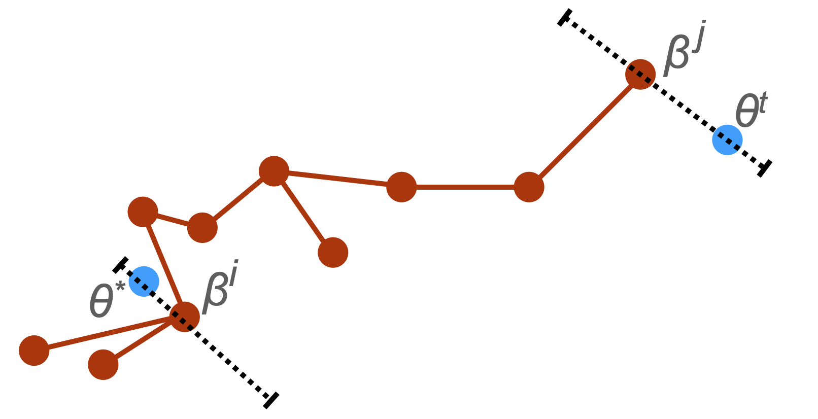
Figure 2: Diagram illustrating the proposal for moving from $\theta^{t}$ (blue on the right) to $\theta^{*}$ (blue on the left): (i) project $\theta^{t}$ to a node on the graph $j=\mathbb{N}(\theta^{t})$ with location attribute $\beta^{j}$, find the line crossing $\theta^{t}$ and $\beta^{j}$; (ii) random walk to node $i$, and find the line interval parallel to $(\theta^{t}-\beta^{j})$, containing $\beta^{i}$ and points $x$ projecting to $\theta^{i}:$ $\mathbb{N}(x)=i$; (iv) sample $\theta^{*}$ from the new interval and accept $\theta^{*}$ via Metropolis-Hastings criterion.

• Find $j=\mathbb{N}(\theta^{t})$, and calculate the directional unit-length vector between $\theta^{t}$ and its projection $\beta^{j}$, $v=(\theta^{t}-\beta^{j})/\|\theta^{t}-\beta^{j}\|$.

• On the line $\{x:x=\beta^{i}+\xi v\}$ with $\xi\in\mathbb{R}$, find the maximum-magnitude $a^{i}$ and $b^{i}$, such that

  $$\mathbb{N}(\beta^{i}+\xi v)=i\;\forall\xi\in(a^{i},b^{i}),-l\leq a^{i}\leq 0,0\leq b^{i}\leq l.$$

• Draw $\theta^{*}$ uniformally from $\{x:x=\beta^{i}+\xi v,a^{i}<\xi<b^{i}\}$.

It is not hard to see that

$$F(\theta^{*}\mid\beta_{i},\theta^{t})=\frac{1}{b^{i}-a^{i}}1\{\|\theta^{*}-\beta^{i}\|\leq l,\mathbb{N}(\theta^{*})=i\},$$

where $l>0$ is a truncation to ensure properness of $F$. We can find the line segment easily using one-dimensional bisection. The acceptance rate in (2) becomes:

$$\min\bigg{[}1,\frac{\Pi(\theta^{*}\mid y)|B(i;r)|^{-1}(b_{i}-a_{i})^{-1}}{\Pi(\theta^{t}\mid y)|B(j;r)|^{-1}(b_{j}-a_{j})^{-1}}\bigg{]}.$$ (4)

We now give a theoretical characterization of the acceptance rate in terms of its rate of change as $p$ grows. For now, we treat the approximate sample size $m$ as a sufficiently large number that satisfies the two assumptions below, and we will discuss the associated requirement on $m$ later.

To obtain a lower bound on the acceptance rate, we first exclude the part of probability corresponding to when we project to $\beta^{j}:\min_{i\in B(j,r)\setminus j}|\log\Pi(\beta^{i}\mid y)-\log\Pi(\beta^{j}\mid y)|>\kappa$ with $\kappa$ the chosen constant in (3). For the remaining $\beta^{j}$’s, we can form an $\delta$-covering, denoted by $\tilde{B}_{1}$. That is, for any $x\in\tilde{B}_{1}$, $\min_{j}\|x-\beta_{j}\|_{2}\leq\delta$. We choose $\delta=c_{2}p^{-c_{3}}$ with $c_{2}>0$ and $-\infty<c_{3}<1/2$.

Next, we assume (A1) there exists set $\tilde{B}_{2}$ and $p$-independent constants $c_{1}>0$ and $\gamma\geq 0$ such that for any $(\theta,\theta^{\prime})\in\tilde{B}_{2}\times\tilde{B}_{2}$,

$$|\log\Pi(\theta\mid y)-\log\Pi(\theta^{\prime}\mid y)|\leq c_{1}p^{\gamma}\|\theta-\theta^{\prime}\|,$$

where $\|\cdot\|$ denotes some norm. This is commonly referred to as a $(c_{1}p^{\gamma})$-smoothness condition (Bubeck, 2015) if one uses Euclidean norm, and recently considered by Tang and Yang (2022, preprint arXiv:2206.06491) in the study of Metropolis-Adjusted Langevin algorithms. The difference compared to Tang and Yang (2022) is that we only impose this condition on a subset $\tilde{B}_{2}\subset\Theta$, hence the condition is relatively easy to satisfy. Taking $\mathcal{B}=\tilde{B}_{1}\cap\tilde{B}_{2}$, (A2) we assume $\mathcal{B}$ has posterior probability $\int_{\mathcal{B}}\Pi(\theta\mid y)d\theta=\mu_{\mathcal{B}}$ bounded away from zero.

Theorem 1.

Under (A1) and (A2), we further assume $(b_{i}-a_{i})/(b_{j}-a_{j})<c_{4}$ for all $i,j:i\in B(j;r)$, $|B(j;r)|\leq c_{5}$ for all $j$, and $l\leq\delta$. Denoting the acceptance in (2) by $\alpha(\theta^{t},\theta^{*})$, we have

$$\mathbb{E}_{\theta^{t}\sim\Pi(\theta\mid y)}\alpha(\theta^{t},\theta^{*})>\frac{\mu_{\mathcal{B}}}{c_{4}c_{5}}e^{-\kappa}\exp\{-2c_{1}p^{(\gamma-c_{3})}\}.$$

Remark 2.

Therefore, with suitable $\gamma$ and $c_{3}<1/2$, we have the acceptance rate vanishing at a rate slower than $O\{\exp(-\tilde{c}p)\}$. We can obtain $\gamma\leq 1/2$ for many commonly seen posterior densities. For example, for $\log\Pi(\theta\mid y)=-\theta^{\prime}A\theta+o(\|\theta\|_{2}^{2})$ with positive definite $A$, we can find a $\tilde{B}_{2}$ inside the ball $\{\theta:\|\theta\|_{1}\leq a_{1}\sqrt{p}\}$ which implies $\|\theta\|_{2}\leq\|\theta\|_{1}\leq a_{1}\sqrt{p}$. In that case, we have $\gamma=1/2$ for the Euclidean norm.

We now discuss the required size $m$ on the approximate samples. Obviously, the larger $m$, the larger area $\tilde{B}_{1}$ and $\mu_{\mathcal{B}}$ will be. To more precisely characterize its dependency on $p$, and suggest choice for $c_{3}$, we can think of a high posterior probability polytope $\mathcal{P}=(\theta:\theta=k_{0}\Sigma^{1/2}_{0}x+a_{0},\|x\|_{1}\leq 1)$ with for some $a_{0}\in\Theta$, $\Sigma_{0}$ positive definite, and some fixed and dimension-independent $k_{0}>0$ so that $\mu_{\mathcal{P}}=\int_{\mathcal{P}}\Pi(\theta\mid y)d\theta\gg 0$. Assuming our approximate sampler can generate points over $\mathcal{P}$, the question is how many balls $(x:\|x-\theta_{j}\|\leq\delta)$ do we need to cover $\mathcal{P}$?

Apparently, the answer depends on the type of norm used in $\|x-\theta_{j}\|$. In the following, we consider using $\|x-\theta_{j}\|_{\Sigma_{0}}=\sqrt{(x-\theta_{j})^{T}\Sigma_{0}^{-1}(x-\theta_{j})}$, which simplifies the problem to the covering a unit $L1$-ball using small $L2$-balls. The celebrated Maurey’s empirical method (Pisier, 1999) shows that, to cover a unit $L1$-ball, we only need at least $m=(2p+1)^{O(1/\delta_{0}^{2})}$-many $\delta_{0}$-$L2$-balls with radius $\delta_{0}$, provided that $\delta_{0}>p^{-1/2}$. With appropriate scaling, we reach the choice of $\delta=c_{2}p^{-c_{3}}$, with $c_{3}<1/2$. Substituting into the lower bound of $m$, we see that $m=(2p+1)^{O(p^{2c_{3}})}$. Therefore, we see that $c_{3}=0$ gives our suggested choice of $m=O(p)$, which balances between controlling acceptance rate decay and preventing excessive demand on the number of approximate samples.

Remark 3.

In the above, we focus on a general high-dimensional setting with a high posterior probability set $\mathcal{P}$. On the other hand, in special but often encountered cases where the high posterior probability set can be found as a $\delta$-neighborhood of a $\tilde{p}$-dimensional set (with $\tilde{p}\ll p$, such as in sparse regression where most elements of $\theta$ are close to $0$), we can change the above paragraph to be based on a $\tilde{p}$-dimensional $L1$-ball. This could lead to a further reduction of $m$.

The reason that we choose to study covering $\mathcal{P}$, an affinely transformed $L1$-ball, instead of an affinely transformed $L2$-ball (ellipsoid), is that the covering number of the unit $L2$-ball with $\delta_{0}$-radius $L2$-balls (each of radius $\delta_{0}<1$) is $m=O(1/\delta_{0})^{p}$ (Vershynin, 2015), which would be excessively large. On the other hand, since traditionally it is more common to think of a high posterior probability as an ellipsoid $\mathcal{E}=(\theta:\theta=k_{0}\Sigma^{1/2}_{0}x+a_{0},\|x\|_{2}\leq 1)$ than polytope $\mathcal{P}=(\theta:\theta=k_{0}\Sigma^{1/2}_{0}x+a_{0},\|x\|_{1}\leq 1)$, we want to give some characterization on the probability of $\mathcal{P}$. We focus on the case when $(\theta\mid y)$ is a $p$-dimensional sub-Gaussian random vector (Vershynin, 2018). We say $x\in\mathbb{R}^{p}$ is a sub-Gaussian random vector, if $\mathbb{E}x=0$ and for any $v\in\mathbb{R}^{p}:\|v\|_{2}=1$, $v^{\rm T}x$ is sub-Gaussian with variance proxy $\sigma^{2}_{0}$, $\text{pr}(v^{\rm T}x\geq d)\leq 2\exp\{-d^{2}/(2\sigma^{2}_{0})\}$ for any $d>0$. With transform $\theta=\Sigma^{1/2}_{0}x+a_{0}$, $\theta$ is sub-Gaussian as well except with a different center and different variance proxy. It is not hard to see that if $x_{\theta}=\Sigma_{0}^{-1/2}(\theta-a_{0})$ is sub-Gaussian random vector with variance proxy $\sigma^{2}_{0}$, then $\text{pr}(\|x_{\theta}\|_{1}\leq d)\geq 1-2\exp\{-{d^{2}}/(2p\sigma^{2}_{0})\}$. This can be obtained by observing $\|x\|_{1}=\tilde{v}^{\prime}x$ for some $\tilde{v}\in(-1,1)^{p}$ and $\|\tilde{v}\|_{2}=\sqrt{p}$. Therefore, the associated $\mathcal{P}$ gives a high probability region.

3 Theory on Accelerated Mixing Time

We now focus on the mixing time of the accelerated algorithm. To provide the necessary background, denote the state space by $\Theta$, and consider a Markov transition kernel $\mathcal{M}$, with $\mathcal{M}(x,\cdot)$ the transition probability measure from state $x$ and $\pi(\cdot)$ the invariant distribution of ${\mathcal{M}}$. Under the context of posterior estimation, we have $\pi(\cdot)$ equal the posterior distribution associated with kernel $\Pi(\theta\mid y)$. We use $\mathcal{M}^{t}(x^{0},\cdot)$ to denote the distribution after $t$ iterations of transitioning via $\mathcal{M}$ with $x^{0}$ the initial point drawn from $\pi^{0}$. Given a small positive number $\eta$, the $\eta$-mixing time of a Markov chain is the smallest $t$ such that the total variation distance satisfies

$$\sup_{A\in\Theta}|\mathcal{M}^{t}(x^{0},A)-\pi(A)|\leq\eta.$$

Since the left-hand side is often intractable, one often derives an upper bound of the left-hand side as a diminishing function of $t$, and produces an upper bound estimate of the mixing time.

Now we review an important concept of “conductance”, which is useful for calculating the above upper bound. Consider an ergodic flow

$$\Phi_{\mathcal{M}}(A)=\int_{x\in A}{\mathcal{M}}(x,A^{c})\,\pi(dx),$$

as the amount of total flow from $A$ to $A^{c}=\Theta\setminus A$. The conductance of $\mathcal{M}$ is a measurement of the bottleneck flow adjusted by the volume:

$$\psi^{*}_{\mathcal{M}}:=\inf_{A\subset\Theta,\pi(A)<1/2}\frac{\Phi_{\mathcal{M}}(A)}{\pi(A)}.$$

The corrollary 3.3 of Lovász and Simonovits (1992) states that $\sup_{A\in\Theta}|\mathcal{M}^{t}(x^{0},A)-\pi(A)|\leq\sqrt{M}\{1-(\psi^{*}_{\mathcal{M}})^{2}/2\}^{t}$, with $M=\sup_{A\subset\Theta}\pi^{0}(A)/\pi(A)$.

Therefore, when comparing two Markov chains, a large conductance $\psi^{*}_{\mathcal{M}}>\psi^{*}_{\mathcal{M}^{\prime}}$ means that $\mathcal{M}$ has a faster-diminishing upper-bound rate on the total variation distance, hence a smaller upper-bound estimate on the mixing time, when compared with $\mathcal{M}^{\prime}$. Although this is not a direct comparison between two mixing times, it offers theoretical insights into why one algorithm empirically shows a faster mixing of Markov chains than the other.

We now focus on the Markov chain generated by the baseline $\mathcal{K}(\theta^{t},\cdot)$. For a sufficiently small $\epsilon>0$, we define an $\epsilon$-expansion from the infimum

$$\mathcal{A}_{\epsilon}^{*}(\mathcal{K}):=\biggl{\{}A\subset\Theta\ \bigg{|}\ \frac{\Phi_{\mathcal{K}}(A)}{\pi(A)}<\psi^{*}_{\mathcal{K}}+\epsilon,\pi(A)<\frac{1}{2}\biggr{\}}.$$

We consider the graph-accelerated Markov chain with $\mathcal{R}=w\mathcal{Q}+(1-w)\mathcal{K}$ where the transition kernel $\mathcal{Q}$ has the same invariant distribution $\pi$. We have the following guarantee.

Theorem 2.

If there exists a sufficiently small $\epsilon>0$, for any $A\in\mathcal{A}_{\epsilon}^{*}(\mathcal{K})$, $\Phi_{\mathcal{Q}}(A)>\Phi_{\mathcal{K}}(A)$, then there exists $w\in(0,1]$ such that $\psi^{*}_{\mathcal{R}}>\psi^{*}_{\mathcal{K}}$.

The above result shows that $\mathcal{Q}$ only needs to improve the ergodic flow on $\mathcal{A}_{\epsilon}^{*}(\mathcal{K})$ where the $\epsilon$-expansion of bottleneck flow of $\mathcal{K}$ happens. This means that as long as $\mathcal{Q}$ improves the flow in $\mathcal{A}_{\epsilon}^{*}(\mathcal{K})$, the mixture kernel $\mathcal{R}$ will have potential acceleration.

Remark 4.

This theoretical result formalizes our comment in Remark 1 — we do not need $\mathcal{Q}$ alone to form a fast-mixing Markov chain. As an intuitive example, for sampling a $k$-modal distribution via the mixture $\mathcal{K}$, including jumps over a “barebone” graph with only $k$ nodes (each located near a unique mode) as $\mathcal{Q}$ will help improve the mixing of Markov chain.

4 Numerical Results

4.1 Sampling Posterior with Non-convex Density Contour

For sampling low-dimensional $\Pi(\theta\mid y)$, the random-walk Metropolis algorithm is appealing due to its low computational cost. For low dimensional problems, a common choice for random walk proposal is $\operatorname{No}(\cdot;\theta^{t},s\,I)$, with $s>0$ the step size. A potential issue is that when the high posterior density region is not close to a convex shape, the step size $s$ would have to be small, leading to computing inefficiency.

The following example is often used as a challenging case (Haario et al., 1999), with likelihood and prior

$$y_{i}\stackrel{{\scriptstyle iid}}{{\sim}}\operatorname{No}(\theta^{2}_{1}+\theta_{2},1^{2}),\text{ for }i=1,\ldots,n,\qquad\theta\sim\operatorname{No}(0,I_{2}).$$

If the true parameters are chosen subject to the constraint $\theta_{1}^{2}+\theta_{2}=1$, the posterior distribution of $(\theta_{1},\theta_{2})$ would spread around the banana-shaped curve $\{(\theta_{1},\theta_{2}):\theta^{2}_{1}+\theta_{2}=1\}$.

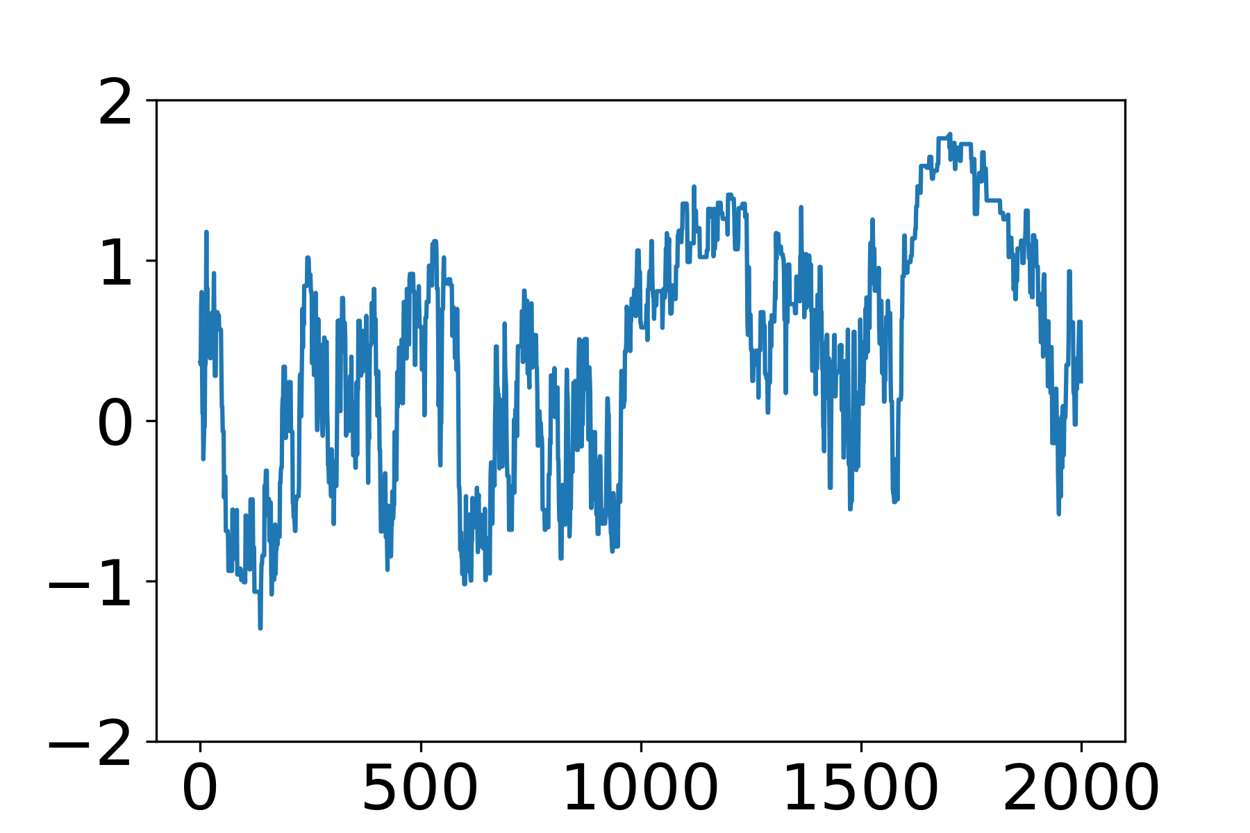
(a) Traceplot of $\theta_{1}$ using random-walk Metropolis.

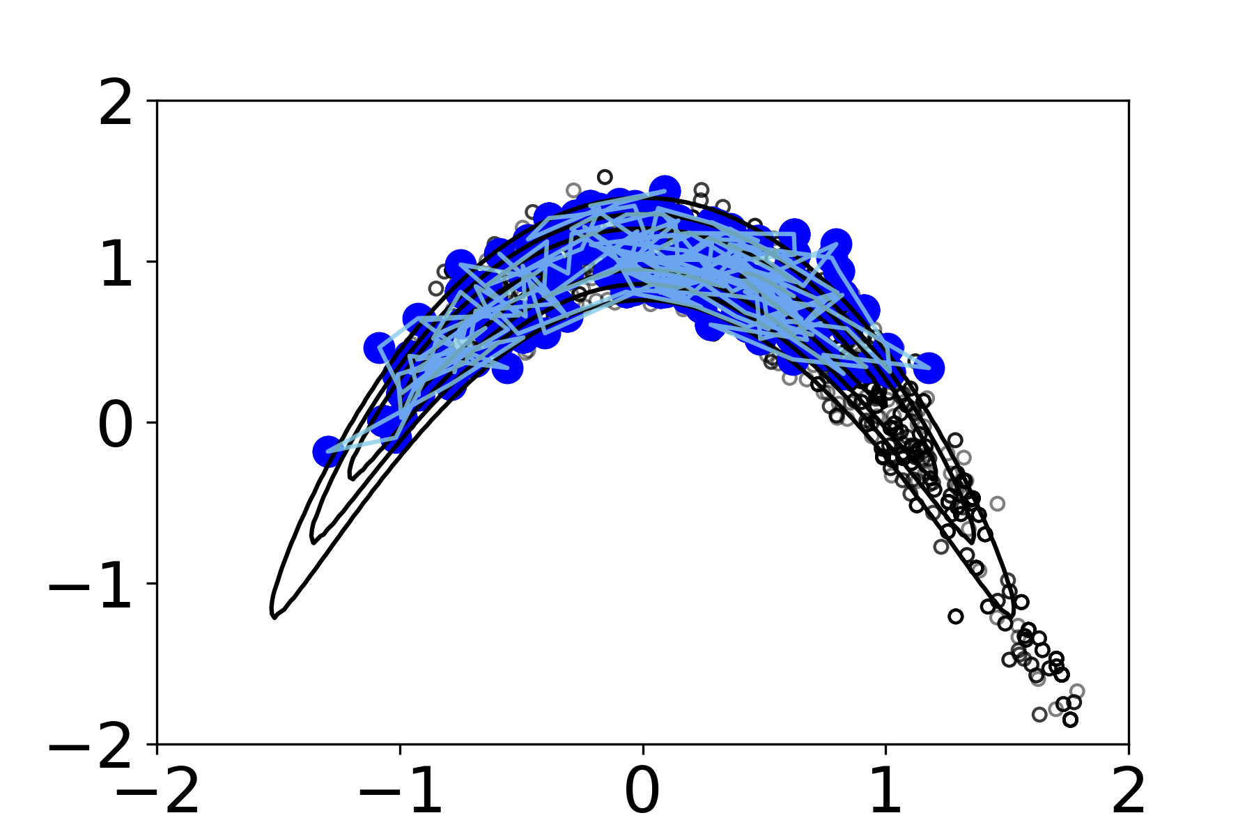
(b) Markov chain sample of $(\theta_{1},\theta_{2})$ from the random-walk Metropolis. The first 400 sample points and traces are shown in blue.

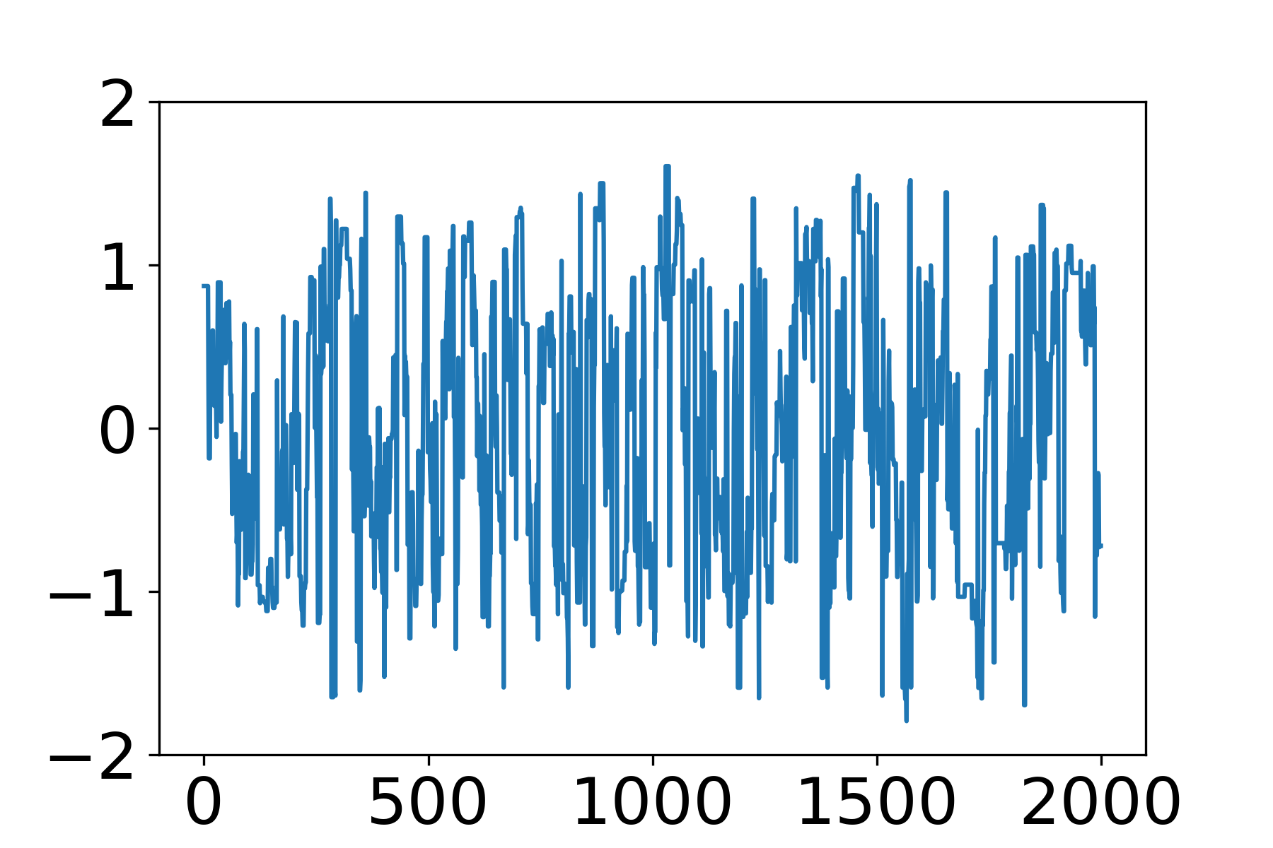
(c) Traceplot of $\theta_{1}$ using the accelerated algorithm.

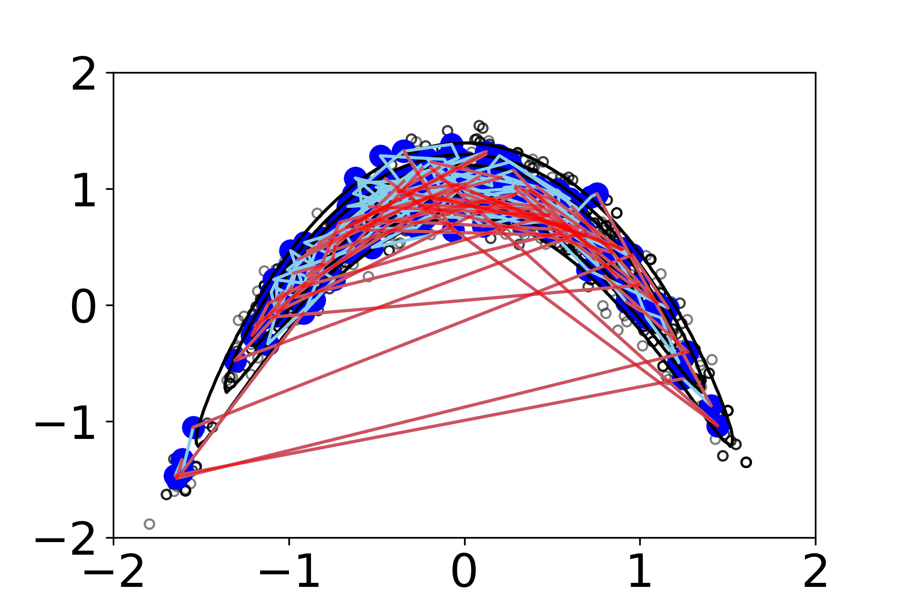
(d) Markov chain sample of $(\theta_{1},\theta_{2})$ from the accelerated algorithm. The first 400 sample points and traces are shown in blue, with successful graph jump steps shown in red.

Figure 3: Graph-accelerated random-walk Metropolis for sampling a posterior distribution of banana shape.

Using random-walk Metropolis as the baseline algorithm, we tweak $s$ to around $0.5$ so that the Metropolis acceptance rate is around 0.234. We run the algorithm for 3000 iterations and use the last 2000 as a Markov chain sample. Figure 3(a)(b) shows that it takes a long time for the sampler to move from one end to the other.

For acceleration, we first obtain $100$ approximate samples from a variational method based on a 10-component Gaussian mixture $\sum_{k=1}^{10}\tilde{w}_{k}\operatorname{No}(\tilde{\mu}_{k},I\tilde{\sigma}^{2})$, then we run the accelerated algorithm. As shown in Figure 3, the accelerated algorithm jumps rapidly between the two ends, leading to improved mixing performance. The effective sample size per iteration for $\theta_{1}$ from the baseline algorithm is 0.16%, while the one for the accelerated version is 6.1%.

4.2 Sampling Posterior with Latent Variables

To show that our algorithm works well in relatively large dimensions, we experiment with a latent Gaussian model for count data. Specifically, we use the power outage count for a zip code area in the south of Florida collected during a 90-day time period in the 2009 hurricane season. There are $n=100$ records of outage counts $y_{i}\in\mathbb{Z}_{\geq 0}$, reported at irregularly-spaced time points. To ease the prior specification, we first rescale the time records to be in $[0,1]$, and denote the transformed time by $t_{i}$. We use the following likelihood based on a negative-binomial latent Gaussian model, with latent Gaussian covariance $\Sigma_{i,j}(\tau,h)=\tau\exp[-(t_{i}-t_{j})^{2}/{2h}]$, leading to augmented likelihood:

$$L(y,z\mid\tau,h)=(2\pi)^{-n/2}|\Sigma(\tau,h)|^{-1/2}\exp\bigg{[}-\frac{1}{2}z^{\rm T}\{\Sigma(\tau,h)\}^{-1}z\bigg{]}\prod_{i=1}^{n}\frac{\exp(rz_{i})}{\{1+\exp(z_{i})\}^{r+y_{i}}}.$$

For prior specification, we use $h\sim\text{Ga}^{-1}(2,1)$ for the bandwidth $h>0$, $r\sim\text{No}_{0,\infty)}(0,1)$ for the inverse dispersion parameter $r>0$, $\tau\sim\text{Ga}^{-1}(2,1)$ for the scale $\tau>0$.

We first describe the baseline algorithm posterior sampling. Using Pólya-Gamma latent variable $\omega_{i}$ (Polson et al., 2013), denoted by $\omega_{i}\sim\text{PG}(\cdot\mid r+y_{i},0)$, we have

$$\frac{\{\exp(z_{i})\}^{r}}{\{1+\exp(z_{i})\}^{r+y_{i}}}=2^{-(r+y_{i})}\exp\{(\frac{r-y_{i}}{2})z_{i}\}\int\exp(-\omega_{i}z^{2}_{i}/2)\text{PG}(\omega_{i}\mid r+y_{i},0)\textup{d}\omega_{i}.$$

We have closed-form updates for most of the latent variables and parameters, $\omega_{i}\sim\text{PG}(r+y_{i},z_{i})$ for $i=1,\ldots,n$, $z\sim\text{No}[\{\Sigma^{-1}+\text{diag}(\omega_{i})\}^{-1}\{(r-y)/2\},\{\Sigma^{-1}+\text{diag}(\omega_{i})\}^{-1}]$ and $\tau\sim\text{Ga}^{-1}\{n/2+2,z^{\rm T}\tilde{\Sigma}^{-1}(h)z/2+1\}$ with $\tilde{\Sigma}_{i,j}(h)=\exp[-(t_{i}-t_{j})^{2}/{2h}]$. On the other hand, since $h$ and $r$ do not have full conditional distribution available in closed form, we use softplus reparameterization $h=\log\{1+\exp(\tilde{h})\}$ and $r=\log\{1+\exp(\tilde{r})\}$ and use random-walk Metropolis algorithm with proposal $\operatorname{No}\{\cdot;(\tilde{h},\tilde{r})^{t},Is\}$ to obtain an update on $(\tilde{h},\tilde{r})\in\mathbb{R}^{2}$, then transform to $(h,r)$. In the random-walk Metropolis algorithm, we use the posterior with $(\tau,\omega)$ integrated out, and tweak $s$ so that the acceptance rate is around 0.234. We run the baseline algorithm for 20,000 iterations, and treat the first 5,000 as burn-in. As shown in Figure 4(a)(b) and (e), the baseline Gibbs sampling algorithm suffers from critically slow mixing. Even at the 100-th lag, most of the parameters and latent variables still show autocorrelations near 40%.

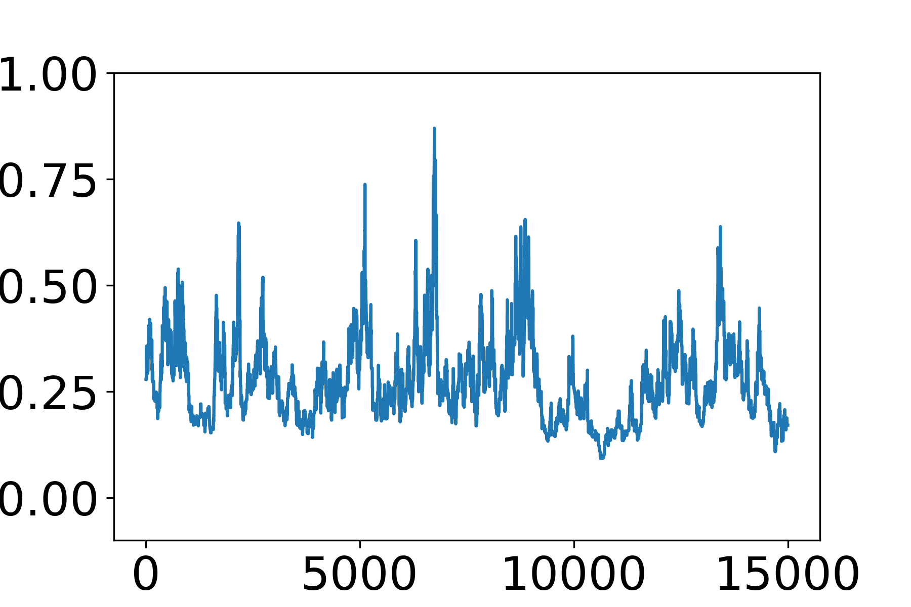
(a) Traceplot of $h$ produced by the Gibbs sampler.

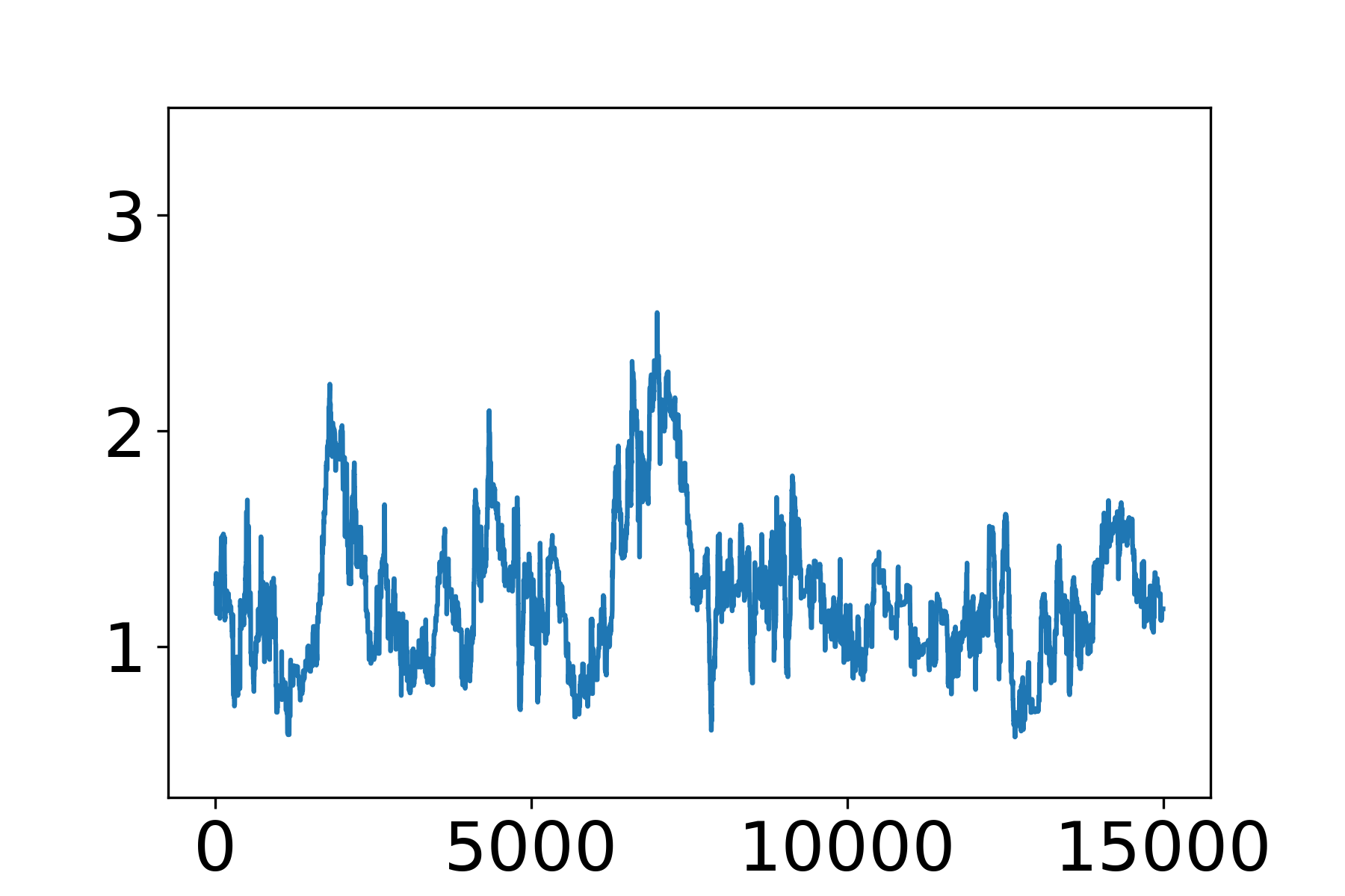
(b) Traceplot of $r$ produced by the Gibbs sampler.

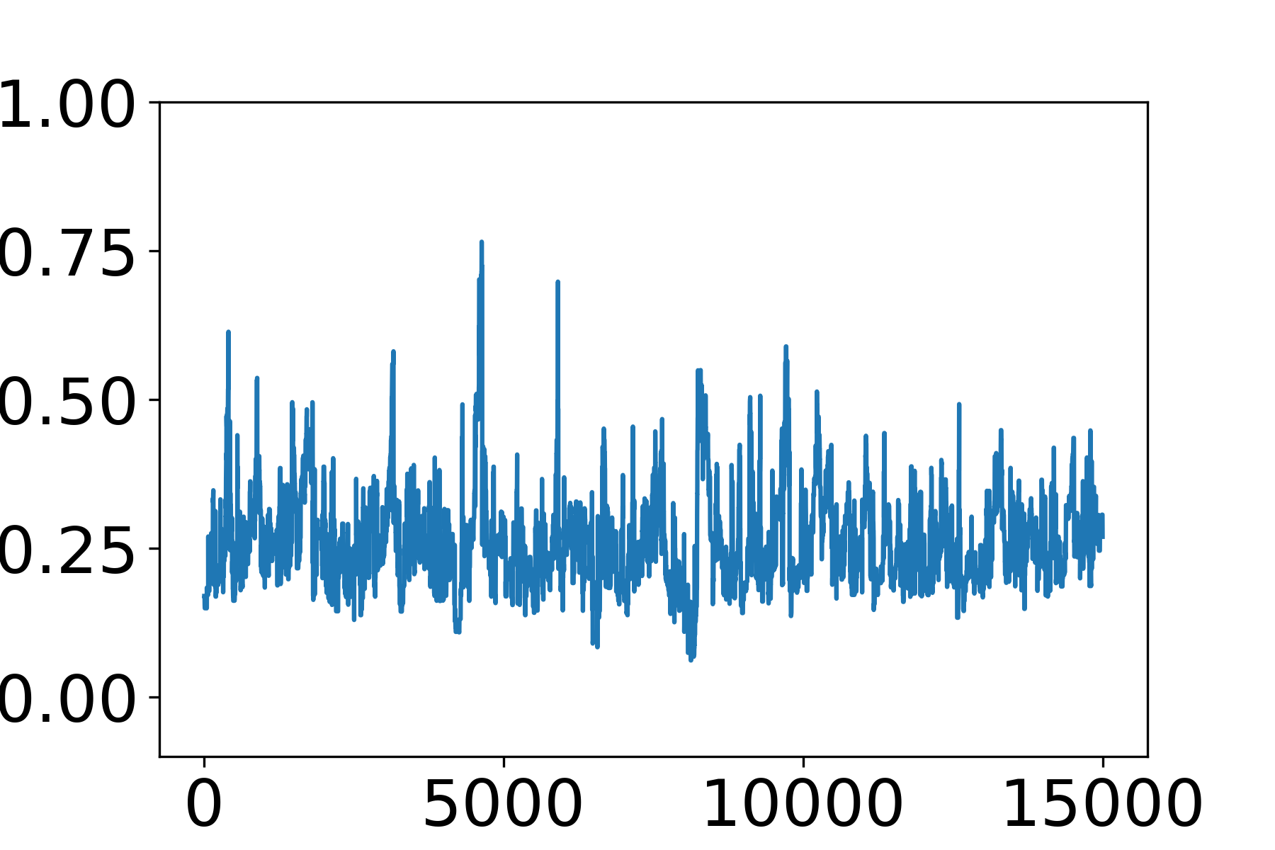
(c) Traceplot of $h$ produced by the accelerated sampler.

(d) Traceplot of $r$ produced by the accelerated sampler.

\begin{overpic}[width=476.98463pt]{lgm_no_acc_acf_boxplot} \put(50.0,-2.0){\scriptsize Lag} \put(-1.0,12.0){\rotatebox{90.0}{\scriptsize Autocorrelation}} \end{overpic}

(e) Autocorrelation plot for all parameters and latent variables, from the samples produced by Gibbs sampler.

\begin{overpic}[width=476.98463pt]{lgm_acc_acf_boxplot} \put(50.0,-3.0){\scriptsize Lag} \put(-1.0,12.0){\rotatebox{90.0}{\scriptsize Autocorrelation}} \end{overpic}

(f) Autocorrelation plot for all parameters and latent variables, from the samples produced by accelerated sampler.

\begin{overpic}[height=93.95122pt,width=346.89731pt]{lgm_ess_boxplot} \put(-3.0,12.0){\rotatebox{90.0}{\scriptsize Effective sample size \%}} \end{overpic}

(g) Boxplots showing effect sample sizes per iteration for two algorithms.

\begin{overpic}[width=455.3023pt]{lgm_figure_acc_theta1v2} \put(50.0,-3.0){\scriptsize$h$} \put(0.0,30.0){\rotatebox{90.0}{\scriptsize$r$}} \end{overpic}

(h) Markov chain sample of $(h,\tau)$ from the accelerated algorithm, with successful graph jumps shown in red.

\begin{overpic}[width=455.3023pt]{lgm_figure_acc_gp_est} \put(50.0,-3.0){\scriptsize$t$} \put(-2.0,30.0){\rotatebox{90.0}{\scriptsize$y$}} \end{overpic}

(i) Posterior estimate of the mean curve using the accelerated algorithm.

Figure 4: Sampling a posterior distribution of a latent Gaussian model for count data.

For the acceleration algorithm, we obtain approximate samples of $\beta^{j}=(z,\tau,h,r)^{j}\in\mathbb{R}^{103}$ by simply taking the first $1,000$ Markov chain samples after the burn-in period from the slow-mixing Gibbs sampler, then we construct the graph and run the accelerated algorithm for 20,000 iterations (with the first 5,000 as burn-in). Despite the relatively large dimension, the graph jump steps had $18.4\%$ of success rate {red lines in Figure 4(h)}. As shown in Figure 4(c)(d) and (f), the accelerated algorithm leads to much-improved mixing performance. Almost all parameters and latent variables have autocorrelations reduce to small values after the 60-th lag. We plot the posterior mean curve $r\exp(-z_{i})$, and the point-wise 95% credible band in Figure 4(i).

5 Discussion

In the above accelerated Markov chain sampling, we treat the graph as a fixed object. An interesting extension to explore is to allow the graph to keep growing, by adding some samples collected from the Markov chain. It remains to be studied on how to ensure the modified and hence non-reversible algorithm converges to target posterior distribution, and whether it leads to further improvement in mixing.

Appendix A Proof of Theorems

A.1 Proof of Theorem 1

Proof.

The acceptance rate under our specified $F(\theta^{*}\mid\beta_{i},\theta^{t})$ is

$$\alpha(\theta^{t},\theta^{*})=\min\bigg{\{}1,\frac{\Pi(\theta^{*}\mid y)|B(i;r)|^{-1}(b_{j}-a_{j})^{-1}}{\Pi(\theta^{t}\mid y)|B(j;r)|^{-1}(b_{i}-a_{i})^{-1}}\bigg{\}}.$$

We see that $\min_{j}\|\theta^{*}-\beta_{j}\|\leq\delta$ by the way we generate $\theta^{*}$, hence $\theta^{*}\in\mathcal{B}$. Consider any $\theta^{t}\in\mathcal{B}$,

$$\log\Pi(\theta^{*}\mid y)-\log\Pi(\theta^{t}\mid y)$$

$$\geq\log\Pi(\theta^{*}\mid y)-\log\Pi(\beta_{i}\mid y)+\log\Pi(\beta_{j}\mid y)-\log\Pi(\theta^{t}\mid y)-|\log\Pi(\beta_{i}\mid y)-\log\Pi(\beta_{j}\mid y)|$$

$$\geq-c_{1}p^{\gamma}(\|\theta^{*}-\beta_{i}\|+\|\theta^{t}-\beta_{j}\|)-\kappa$$

$$\geq-2c_{1}p^{\gamma}\delta-\kappa.$$

Since we know $B(j;r)\geq 1$, we have $|B(j;r)|/|B(i;r)|\leq c_{5}$. Including the bound ratio $(b_{i}-a_{i})/(b_{j}-a_{j})<c_{4}$, and taking expectation over $\theta^{t}\sim\Pi(\theta\mid y)$ yields the result. ∎

A.2 Proof of Theorem 2

Proof.

We consider the conductance under two cases:

1) Transitioning from $A\in\mathcal{A}_{\epsilon}^{*}(\mathcal{K})$:

For any $A\in\mathcal{A}_{\epsilon}^{*}(\mathcal{K})$, we have for any $w\in(0,1]$:

$$\begin{aligned} \frac{\Phi_{\mathcal{R}}(A)}{\pi(A)}=\frac{w\Phi_{\mathcal{Q}}(A)+(1-w)\Phi_{\mathcal{K}}(A)}{\pi(A)}>\frac{\Phi_{\mathcal{K}}(A)}{\pi(A)}\geq\psi^{*}_{\mathcal{K}}.\end{aligned}$$ (5)

2) Transitioning from $B\in\Theta\setminus\mathcal{A}_{\epsilon}^{*}(\mathcal{K})$:

For any $B\in\mathcal{B}=\{A\in\Theta:\pi(A)<1/2,A\not\in\mathcal{A}_{\epsilon}^{*}(\mathcal{K})\}$, we have $\Phi_{\mathcal{K}}(B)/\pi(B)\geq\psi_{\mathcal{K}}^{*}+\epsilon$.

Let $m_{\mathcal{B}}:=\inf_{B\in\mathcal{B}}\Phi_{\mathcal{Q}}(B)/\Phi_{\mathcal{K}}(B)\geq 0$, and for any $w\in(0,1]$ such that:

$$w(1-m_{\mathcal{B}})<\frac{\epsilon}{\psi^{*}_{\mathcal{K}}+\epsilon},$$ (6)

we have

$$\begin{aligned} &\frac{\Phi_{\mathcal{R}}(B)}{\pi(B)}=\frac{w\Phi_{\mathcal{Q}}(B)+(1-w)\Phi_{\mathcal{K}}(B)}{\pi(B)}=\{w\Phi_{\mathcal{Q}}(B)/\Phi_{\mathcal{K}}(B)+(1-w)\}\frac{\Phi_{\mathcal{K}}(B)}{\pi(B)}\\ &\geq\{wm_{\mathcal{B}}+(1-w)\}\frac{\Phi_{\mathcal{K}}(B)}{\pi(B)}>\frac{\psi^{*}_{\mathcal{K}}\Phi_{\mathcal{K}}(B)}{(\psi_{\mathcal{K}}^{*}+\epsilon)\pi(B)}\geq\psi^{*}_{\mathcal{K}}.\end{aligned}$$ (7)

To show that such a $w$ always exists, as well as choosing a large value for $w$: when $m_{\mathcal{B}}\geq 1$, we can choose $w=1$; when $m_{\mathcal{B}}<1$, we can choose $w=(1-m_{\mathcal{B}})^{-1}{\epsilon}/(\psi^{*}_{\mathcal{K}}+\epsilon)-\eta$, with $\eta>0$ sufficiently small so that $w>0$.

Combining 1) and 2), we see that there exists $w\in(0,1]$, such that $\psi^{*}_{\mathcal{R}}>\psi^{*}_{\mathcal{K}}$. ∎

Appendix B Optimization Algorithm for Further Improvement on Graph Choice

We provide the details on the optimization of a random walk transition probability matrix $P$. One solution is using the dual ascent algorithm. The minimization of spectral norm is equivalent to:

$$\min_{P,s} \;s$$

subject to $$\|P-1_{m}\pi^{\rm T}_{\beta}\|_{2}\leq s,\;s\geq 0$$

$$P1_{m}=1_{m},\qquad\pi_{\beta}^{\rm T}P=\pi^{\rm T}_{\beta},$$

$$P_{i,j}=0\text{ if }(i\to j)\not\in E_{\bar{G}},\qquad P_{i,j}\geq 0$$

Using semi-definite programming, we can set up the Lagrangian:

$$\mathcal{L}(P,Z,s,u,v,Y,\lambda)= s-\text{tr}\bigg{\{}\begin{bmatrix}Z_{11}&Z_{12}\\ Z^{\rm T}_{12}&Z_{22}\end{bmatrix}\begin{bmatrix}sI&(P-1_{m}\pi^{\rm T}_{\beta})\\ (P-1_{m}\pi^{\rm T}_{\beta})^{\rm T}&sI\end{bmatrix}\bigg{\}}$$

$$+u^{\rm T}(P1_{m}-1_{m})+(\pi_{\beta}^{\rm T}P-\pi^{\rm T}_{\beta})v-\text{tr}(YP)-\lambda s.$$

where $Z\succeq 0$ is a four-block positive semi-definite matrix, $u\in\mathbb{R}^{p}$, $v\in\mathbb{R}^{p}$, $\lambda\geq 0$, lastly, $Y\in\mathbb{R}^{p\times p}$, except $Y_{i,j}\geq 0$ if $(i\to j)\in E_{\bar{G}}$. Clearly, the Lagrangian dual $\inf_{P,s}\mathcal{L}(\cdot)$ would be $-\infty$, unless:

$$-2Z_{12}^{\rm T}+1_{m}u^{\rm T}+v\pi_{\beta}^{\rm T}-Y=0,$$

$$1-\text{tr}(Z)-\lambda=0,$$

which are equivalent to dual feasibility conditions:

$$Z_{12}(j,i)\leq\frac{u_{j}+v_{i}\pi_{\beta}(j)}{2}\text{ if }(i\to j)\in E_{\bar{G}},$$

$$\text{tr}(Z)\leq 1,\;Z\succeq 0$$

for the dual problem:

$$\sup_{Z,u,v}2\text{tr}\big{\{}Z^{\rm T}_{12}(1_{m}\pi^{\rm T}_{\beta})\big{\}}-u^{\rm T}1_{m}-\pi^{\rm T}_{\beta}v.$$

We parameterize $Z=\tilde{Z}\tilde{Z}^{\rm T}$, with $\tilde{Z}\in\mathbb{R}^{p\times p}$, and use log-barrier to enforce inequalities, then use gradient ascent algorithm {via the JAX package (Bradbury et al., 2018)} to find out $\hat{Z},\hat{u},\hat{v}$. Then using complementary slackness condition $s\cdot\text{tr}(Z_{11}+Z_{22})+2\text{tr}\{Z_{12}^{\rm T}(P-1_{m}\pi^{\rm T}_{\beta})\}=0$ and primal optimal condition $s=\|P-1_{m}\pi^{\rm T}_{\beta}\|_{2}$, we can find out the value of $\hat{P}$. We provide numerical illustration in the supplementary material.

Supplementary material

S.1 Numerical illustration on different choices of graph

For numerical illustration, we use the Gaussian mixture example we consider in the main text. In addition to (i) the baseline random walk Metropolis and (ii) the accelerated algorithm with spanning tree graph under default value $(r=1,\kappa=1)$, we experiment with (iii) the accelerated algorithm with greedy optimization on $(r,\kappa)$ to maximize the expected squared jumped distance (with $r=5$ and $\kappa=0.65$), and (iv) the accelerated algorithm using optimized random walk (with edges excluded if $\|\beta^{i}-\beta^{j}\|\leq 0.5$). For (ii)(iii) and (iv), we use the same collection of $m=100$ samples, and we compare the mixing performance of those algorithm via the traceplot of $\theta_{2}$ in Figure 5. As can be seen, (iii) and (iv) further improve the mixing compared to (ii), although these two extensions are much more complicated.

\begin{overpic}[width=433.62pt]{comp_gmm_rw} \end{overpic}

(a) Traceplot of $\theta_{2}$ using random-walk Metropolis.

\begin{overpic}[width=433.62pt]{comp_gmm_acc1} \end{overpic}

(b) Traceplot of $\theta_{2}$ using accelerated algorithm with spanning tree graph with $r=1$, $\kappa=1$.

\begin{overpic}[width=433.62pt]{comp_gmm_acc2} \end{overpic}

(c) Traceplot of $\theta_{2}$ using acceleration via spanning tree graph with greedily optimized $(r,\kappa)$.

\begin{overpic}[width=433.62pt]{comp_gmm_acc3} \end{overpic}

(d) Traceplot of $\theta_{2}$ using acceleration via optimized random walk graph.

Figure 5: Comparing acceleration algorithms using different graphs, for sampling a two-component Gaussian mixture distribution.

S.2 Estimate on the vanishing rate of acceptance probability of Gaussian random-walk Metropolis algorithm

It has been shown (Gelman et al., 1997; Roberts and Rosenthal, 2001) that for Gaussian random-walk Metropolis algorithm with target distribution consisting of $p$ independent components, one may use a Gaussian proposal with standard deviation at $cp^{-1/2}$, so that the acceptance rate could stay above zero and converge to $2\Phi(-\tilde{m}c)$ as $p\to\infty$, with some $\tilde{m}>0$ depending on the target distribution and $\Phi$ the standard Gaussian cumulative distribution function. To roughly estimate the vanishing speed of the acceptance rate under a fixed step size, we can replace $c$ by $cp^{1/2}$ and obtain $2\Phi(-\tilde{m}cp^{1/2})$.

For $x>0$ and $t>x$, $\Phi(-x)=(2\pi)^{-1/2}\int_{x}^{\infty}\exp(-t^{2}/2)\textup{d}t\leq(2\pi)^{-1/2}\int_{x}^{\infty}(t/x)\exp(-t^{2}/2)\textup{d}t=(2\pi)^{-1/2}\exp(-x^{2}/2)/x$. Plugging $x=mcp^{1/2}$ yields $O(p^{-1/2}\exp\{-\tilde{c}p)\}$ for some constant $\tilde{c}>0$. Omitting the dominated $p^{-1/2}$ leads to the $O(\exp\{-\tilde{c}p)\}$ rate.

S.3 Software

The software is hosted and maintained on github repository under the following link
https://github.com/leoduan/graph_acc_mcmc.

References

- Betancourt et al. (2017) Betancourt, M., S. Byrne, S. Livingstone, and M. Girolami (2017). The Geometric Foundations of Hamiltonian Monte Carlo. Bernoulli 23(4A), 2257 – 2298.
- Bierkens et al. (2019) Bierkens, J., P. Fearnhead, and G. Roberts (2019). The Zig-Zag Process and Super-Efficient Sampling for Bayesian Analysis of Big Data. The Annals of Statistics 47(3), 1288 – 1320.
- Blei et al. (2017) Blei, D. M., A. Kucukelbir, and J. D. McAuliffe (2017). Variational Inference: A Review for Statisticians. Journal of the American Statistical Association 112(518), 859–877.
- Boyd et al. (2004) Boyd, S., P. Diaconis, and L. Xiao (2004). Fastest Mixing Markov Chain on a Graph. SIAM Review 46(4), 667–689.
- Bradbury et al. (2018) Bradbury, J., R. Frostig, P. Hawkins, M. J. Johnson, C. Leary, D. Maclaurin, G. Necula, A. Paszke, J. VanderPlas, S. Wanderman-Milne, and Q. Zhang (2018). JAX: Composable transformations of Python+NumPy programs.
- Bubeck (2015) Bubeck, S. (2015, November). Convex Optimization: Algorithms and Complexity. Foundations and Trends® in Machine Learning 8(3–4), 231–357.
- Campbell and Li (2019) Campbell, T. and X. Li (2019). Universal Boosting Variational Inference. Advances in Neural Information Processing Systems 32.
- Chib and Carlin (1999) Chib, S. and B. P. Carlin (1999). On MCMC Sampling in Hierarchical Longitudinal Models. Statistics and Computing 9(1), 17–26.
- Costa and Dufour (2008) Costa, O. L. and F. Dufour (2008). Stability and Ergodicity of Piecewise Deterministic Markov Processes. SIAM Journal on Control and Optimization 47(2), 1053–1077.
- Dalalyan (2017) Dalalyan, A. S. (2017). Theoretical Guarantees for Approximate Sampling From Smooth and Log-Concave Densities. Journal of the Royal Statistical Society Series B: Statistical Methodology 79(3), 651–676.
- Duan et al. (2020) Duan, L. L., A. L. Young, A. Nishimura, and D. B. Dunson (2020). Bayesian Constraint Relaxation. Biometrika 107(1), 191–204.
- Dupont et al. (2019) Dupont, E., A. Doucet, and Y. W. Teh (2019). Augmented Neural ODEs. In Advances in Neural Information Processing Systems, Volume 32.
- Durmus et al. (2020) Durmus, A., É. Moulines, and E. Saksman (2020). Irreducibility and Geometric Ergodicity of Hamiltonian Monte Carlo.
- Durmus et al. (2017) Durmus, A., G. O. Roberts, G. Vilmart, and K. C. Zygalakis (2017). Fast Langevin based algorithm for MCMC in high dimensions. The Annals of Applied Probability 27(4), 2195–2237.
- Fearnhead et al. (2018) Fearnhead, P., J. Bierkens, M. Pollock, and G. O. Roberts (2018). Piecewise Deterministic Markov Processes for Continuous-Time Monte Carlo. Statistical Science 33(3), 386–412.
- Gabrié et al. (2022) Gabrié, M., G. M. Rotskoff, and E. Vanden-Eijnden (2022). Adaptive Monte Carlo Augmented with Normalizing Flows. Proceedings of the National Academy of Sciences 119(10), e2109420119.
- Gelfand (2000) Gelfand, A. E. (2000). Gibbs Sampling. Journal of the American Statistical Association 95(452), 1300–1304.
- Gelfand et al. (1992) Gelfand, A. E., A. F. Smith, and T.-M. Lee (1992). Bayesian Analysis of Constrained Parameter and Truncated Data Problems Using Gibbs Sampling. Journal of the American Statistical Association 87(418), 523–532.
- Gelman (2004) Gelman, A. (2004). Parameterization and Bayesian Modeling. Journal of the American Statistical Association 99(466), 537–545.
- Gelman et al. (1997) Gelman, A., W. R. Gilks, and G. O. Roberts (1997). Weak Convergence and Optimal Scaling of Random Walk Metropolis Algorithms. The Annals of Applied Probability 7(1), 110–120.
- Giordano et al. (2018) Giordano, R., T. Broderick, and M. I. Jordan (2018). Covariances, Robustness and Variational Bayes. Journal of Machine Learning Research 19(51).
- Girolami and Calderhead (2011) Girolami, M. and B. Calderhead (2011). Riemann Manifold Langevin and Hamiltonian Monte Carlo Methods. Journal of the Royal Statistical Society: Series B (Statistical Methodology) 73(2), 123–214.
- Haario et al. (1999) Haario, H., E. Saksman, and J. Tamminen (1999). Adaptive Proposal Distribution for Random Walk Metropolis Algorithm. Computational Statistics 14, 375–395.
- Hoffman et al. (2018) Hoffman, M., P. Sountsov, J. V. Dillon, I. Langmore, D. Tran, and S. Vasudevan (2018). Neutra-Lizing Bad Geometry in Hamiltonian Monte Carlo Using Neural Transport. In Symposium on Advances in Approximate Bayesian Inference, pp. 1–6.
- Johndrow et al. (2020) Johndrow, J., P. Orenstein, and A. Bhattacharya (2020). Scalable Approximate MCMC Algorithms for the Horseshoe Prior. Journal of Machine Learning Research 21(73).
- Johndrow et al. (2019) Johndrow, J. E., A. Smith, N. Pillai, and D. B. Dunson (2019). MCMC for Imbalanced Categorical Data. Journal of the American Statistical Association 114(527), 1394–1403.
- Jones et al. (2014) Jones, G. L., G. O. Roberts, and J. S. Rosenthal (2014). Convergence of Conditional Metropolis-Hastings Samplers. Advances in Applied Probability 46(2), 422–445.
- Kong and Chaudhuri (2020) Kong, Z. and K. Chaudhuri (2020). The Expressive Power of a Class of Normalizing Flow Models. In International Conference on Artificial Intelligence and Statistics, pp. 3599–3609. PMLR.
- Kruskal (1956) Kruskal, J. B. (1956). On the Shortest Spanning Subtree of a Graph and the Traveling Salesman Problem. Proceedings of the American Mathematical Society 7(1), 48–50.
- Lovász and Simonovits (1992) Lovász, L. and M. Simonovits (1992). On the Randomized Complexity of Volume and Diameter. In Proceedings., 33rd Annual Symposium on Foundations of Computer Science, pp. 482–492. IEEE Computer Society.
- Lu and Lu (2020) Lu, Y. and J. Lu (2020). A Universal Approximation Theorem of Deep Neural Networks for Expressing Probability Distributions. Advances in Neural Information Processing Systems 33, 3094–3105.
- Ma et al. (2021) Ma, Y.-A., N. S. Chatterji, X. Cheng, N. Flammarion, P. L. Bartlett, and M. I. Jordan (2021). Is There an Analog of Nesterov Acceleration for Gradient-Based MCMC? Bernoulli 27(3), 1942 – 1992.
- Miller et al. (2017) Miller, A. C., N. J. Foti, and R. P. Adams (2017). Variational Boosting: Iteratively Refining Posterior Approximations. In International Conference on Machine Learning, pp. 2420–2429. PMLR.
- Murota (1998) Murota, K. (1998). Discrete Convex Analysis. Mathematical Programming 83(1-3), 313–371.
- Natarovskii et al. (2021) Natarovskii, V., D. Rudolf, and B. Sprungk (2021). Geometric Convergence of Elliptical Slice Sampling. In International Conference on Machine Learning, pp. 7969–7978. PMLR.
- Neal (2003) Neal, R. M. (2003). Slice Sampling. The Annals of Statistics 31(3), 705–767.
- Papamakarios et al. (2021) Papamakarios, G., E. Nalisnick, D. J. Rezende, S. Mohamed, and B. Lakshminarayanan (2021). Normalizing Flows for Probabilistic Modeling and Inference. The Journal of Machine Learning Research 22(1), 2617–2680.
- Papaspiliopoulos et al. (2007) Papaspiliopoulos, O., G. O. Roberts, and M. Sköld (2007). A General Framework for the Parametrization of Hierarchical Models. Statistical Science, 59–73.
- Pasarica and Gelman (2010) Pasarica, C. and A. Gelman (2010). Adaptively Scaling the Metropolis Algorithm Using Expected Squared Jumped Distance. Statistica Sinica, 343–364.
- Phan et al. (2019) Phan, D., N. Pradhan, and M. Jankowiak (2019). Composable Effects for Flexible and Accelerated Probabilistic Programming in NumPyro. In Program Transformations for ML Workshop at NeurIPS 2019.
- Pisier (1999) Pisier, G. (1999). The Volume of Convex Bodies and Banach Space Geometry, Volume 94. Cambridge University Press.
- Polson et al. (2013) Polson, N. G., J. G. Scott, and J. Windle (2013). Bayesian Inference for Logistic Models Using Pólya–Gamma Latent Variables. Journal of the American Statistical Association 108(504), 1339–1349.
- Pompe et al. (2020) Pompe, E., C. Holmes, and K. Łatuszyński (2020). A Framework for Adaptive MCMC Targeting Multimodal Distributions. The Annals of Statistics 48(5), 2930 – 2952.
- Presman and Xu (2023) Presman, R. and J. Xu (2023). Distance-to-Set Priors and Constrained Bayesian Inference. In International Conference on Artificial Intelligence and Statistics, pp. 2310–2326. PMLR.
- Prim (1957) Prim, R. C. (1957). Shortest Connection Networks and Some Generalizations. The Bell System Technical Journal 36(6), 1389–1401.
- Roberts and Polson (1994) Roberts, G. O. and N. G. Polson (1994). On the Geometric Convergence of the Gibbs Sampler. Journal of the Royal Statistical Society: Series B (Methodological) 56(2), 377–384.
- Roberts and Rosenthal (1998) Roberts, G. O. and J. S. Rosenthal (1998). Optimal Scaling of Discrete Approximations to Langevin Diffusions. Journal of the Royal Statistical Society: Series B (Statistical Methodology) 60(1), 255–268.
- Roberts and Rosenthal (1999) Roberts, G. O. and J. S. Rosenthal (1999). Convergence of Slice Sampler Markov Chains. Journal of the Royal Statistical Society: Series B (Statistical Methodology) 61(3), 643–660.
- Roberts and Rosenthal (2001) Roberts, G. O. and J. S. Rosenthal (2001). Optimal Scaling for Various Metropolis-Hastings Algorithms. Statistical Science 16(4), 351–367.
- Roberts and Rosenthal (2004) Roberts, G. O. and J. S. Rosenthal (2004). General State Space Markov Chains and MCMC Algorithms.
- Roberts and Smith (1994) Roberts, G. O. and A. F. Smith (1994). Simple Conditions for the Convergence of the Gibbs Sampler and Metropolis-Hastings Algorithms. Stochastic Processes and Their Applications 49(2), 207–216.
- Roberts and Tweedie (1996) Roberts, G. O. and R. L. Tweedie (1996). Exponential Convergence of Langevin Distributions and Their Discrete Approximations. Bernoulli, 341–363.
- Rue et al. (2009) Rue, H., S. Martino, and N. Chopin (2009). Approximate Bayesian Inference for Latent Gaussian Models by Using Integrated Nested Laplace Approximations. Journal of the Royal Statistical Society Series B: Statistical Methodology 71(2), 319–392.
- Tanner and Wong (1987) Tanner, M. A. and W. H. Wong (1987). The Calculation of Posterior Distributions by Data Augmentation. Journal of the American Statistical Association 82(398), 528–540.
- Toth et al. (2020) Toth, P., D. J. Rezende, A. Jaegle, S. Racanière, A. Botev, and I. Higgins (2020). Hamiltonian Generative Networks. In International Conference on Learning Representations.
- Vershynin (2015) Vershynin, R. (2015). Estimation in High Dimensions: A Geometric Perspective. In Sampling Theory, a Renaissance: Compressive Sensing and Other Developments, pp. 3–66. Springer.
- Vershynin (2018) Vershynin, R. (2018). High-Dimensional Probability: An Introduction with Applications in Data Science, Volume 47. Cambridge university press.
- Vono et al. (2022) Vono, M., D. Paulin, and A. Doucet (2022). Efficient MCMC Sampling with Dimension-Free Convergence Rate Using ADMM-type Splitting. The Journal of Machine Learning Research 23(1), 1100–1168.
- Yi et al. (2023) Yi, S.-Y., Z. Liu, M.-Q. Liu, and Y.-D. Zhou (2023). Global Likelihood Sampler for Multimodal Distributions. Journal of Computational and Graphical Statistics, 927–937.