Harnack inequalities
for kinetic integral equations

Abstract.

We deal with a wide class of kinetic equations,

$$\big{[}\partial_{t}+v\cdot\nabla_{x}\big{]}f=\mathcal{L}_{v}f.$$

Above, the diffusion term $\mathcal{L}_{v}$ is an integro-differential operator, whose nonnegative kernel is of fractional order $s\in(0,1)$ having merely measurable coefficients. Amongst other results, we are able to prove that nonnegative weak solutions $f$ do satisfy

$$\sup_{Q^{-}}f\ \leq\ c\inf_{Q^{+}}f,$$

where $Q^{\pm}$ are suitable slanted cylinders. No a-priori boundedness is assumed, as usually in the literature, since we are also able to prove a general interpolation inequality in turn giving local boundedness which is valid even for weak subsolutions with no sign assumptions.

To our knowledge, this is the very first time that a strong Harnack inequality is proven for kinetic integro-differential-type equations.
A new independent result, a Besicovitch-type covering argument for very general kinetic geometries, is also stated and proved.

1. Introduction

In the present paper we prove Harnack-type inequalities for weak solutions to the following class of kinetic integro-differential equations,

(1.1) $$\partial_{t}f+v\cdot\nabla_{x}f=\mathcal{L}_{v}f\quad\mbox{in}~{}\varOmega\subset\mathds{R}\times\mathds{R}^{n}\times\mathds{R}^{n}\,,$$

where the diffusion term $\mathcal{L}_{v}$ is given by

(1.2) $$\mathcal{L}_{v}f(t,x,v)=\displaystyle\ {\rm p.~{}\!v.}\!\int_{\mathds{R}^{n}}\!\big{(}f(t,x,w)-f(t,x,v)\big{)}K(w,v)\,{\rm d}w\,,$$

with $K=K(w,v)\approx|w-v|^{-n-2s}$ being a symmetric kernel of order $s\in(0,1)$ with merely measurable coefficients, whose prototype is the classical fractional Laplacian operator  $(-\varDelta_{v})^{s}$, with respect to the $v$-variables, given by

(1.3) $$(-\varDelta_{v})^{s}f(t,x,v):=c_{n,s}\ {\rm p.~{}\!v.}\!\int_{\mathds{R}^{n}}\frac{f(t,x,v)-f(t,x,w)}{\lvert v-w\rvert^{n+2s}}\,{\rm d}w\,.$$

In the display above, $c_{n,s}$ is a positive constant only depending on the dimension $n$ and the differentiability exponent $s$; see [17, Section 2] for further details. We also notice that the integrals in (1.2)-(1.3) may be singular at the origin and they must be interpreted in the appropriate sense. Since we assume that the coefficients in (1.2) are merely measurable, the related equation has to have a suitable weak formulation; we immediately refer the reader to Section 2 below for the precise assumptions on the involved quantities.

During the last century the validity of the classical Harnack inequality has been an open problem in the nonlocal setting, and more in general for integro-differential operators. The first answer, for the purely fractional Dirichlet equation, has been eventually given by Kaßmann in his breakthrough papers [24, 25], where the strong Harnack inequality is proven to be still valid by adding an extra term, basically a natural tail-type contribution on the right-hand side which cannot be dropped nor relaxed even in the most simple case when $\mathcal{L}_{v}$ does coincide with the fractional Laplacian operator $(-\varDelta_{v})^{s}$ in (1.3); see Theorem 1.2 in [24]. Such an extra term does completely disappear in the case of nonnegative weak solutions; see Theorem 3.1 in [25], so that one falls in the classical strong Harnack formulation.

After the breakthrough results by Kaßmann, Harnack-type inequalities and a quite comprehensive nonlocal De Giorgi-Nash-Moser theory have been presented in more general integro-differential elliptic frameworks, even for nonlinear fractional equations. The literature is really too wide to attempt any comprehensive list here; we refer to [15, 31, 16, 6, 7, 29, 19] and the references therein; it is worth presenting also the important Harnack inequalities in [27], which deals with very irregular integro-differential kernels so that a link to Boltzmann-type collision kernels seems veritably close.

The situation becomes more convoluted in the integro-differential parabolic framework. Indeed, in order to prove Harnack-type results, the intrinsic scaling of the involving cylinders will depend not only on the time variable $t$, as in the classical pioneering work by DiBenedetto [14], but also on the differentiability order $s$. This is not for free, as one can imagine, even for the purely $p$-fractional heat equation. A few fractional parabolic Harnack inequalities are however still available, in the case when the kernel of the leading operator is a sort of $(s,2)$-Gagliardo-type one, as, e. g., in [44] in part extending the results in the elliptic counterpart in [15]; see also [26], and the very recent paper [28] together with the aforementioned paper [27] dealing with very intricate irregular kernels. Nevertheless, notable differences in such a parabolic framework inevitably arise, and the validity of a (strong ) Harnack inequality could fail depending on the specific assumptions on the involved kernels, even when starting from bounded solutions; see, e. g., [4, 5].

As noticed above, already in the nonlocal parabolic framework – that to some extents should be seen as the space homogeneous version of (1.1) – one needs new strategies and ideas (see, as a concrete example, the fine analysis in [42]), and strong Harnack inequalities are still not assured (as in the case of the aforementioned counter-examples). More specifically, even for purely kinetic equations with fractional diffusion as in (1.1) the validity or not of a strong Harnack inequality has been an open problem. This is not a surprise because of the very form of the equations in (1.1) which also involves a transport term, and the nonlocality in velocity has to be dealt keeping into account the involuted intrinsic scalings naturally arising. Indeed, to our knowledge, there is still no strong Harnack inequality in the whole integro-differential kinetic panorama, even when the nonnegative solutions are assumed to be bounded a priori, and/or under other assumptions in clear accordance (or not) with some related physical models.

In order to clarify the current situation, it is enlightening to focus on a fundamental class of nonlocal kinetic equations; i. ​e., those modeling the Boltzmann problem without cut-off, for which very important estimates and regularity results have been recently proven, via fine variational techniques and radically new approaches. An inspiring step in such an advance in the regularity theory relies in the approach proposed in the breakthrough paper [32], where the authors, amongst other results, are able to derive a weak Harnack inequality for solutions to a very large class of kinetic integro-differential equations as in (1.1) with very mild assumptions on the integral diffusion in velocity having degenerate kernels $K$ in (1.2) which are not symmetric (not in the usual way) nor pointwise bounded by Gagliardo-type kernels; see Theorem 1.6 there. Under a coercivity condition on $\mathcal{L}_{v}$ and other natural assumptions (see Section 1.1 in [32]), the same result for the Boltzmann equation mentioned above follows as a corollary. Further related regularity estimates under conditional assumptions on the solutions $f$ have been subsequently proven in [34]. Despite the fine estimates and the new approach in [32, 34], a strong Harnack inequality is still missing. A very recent step in this direction, which is worth to be presented, is the following inequality obtained in the interesting paper [37] via a quantitative De Giorgi-type approach based on (local) trajectories, by assuming the solutions $f$ to be globally bounded a priori,

(1.4) $$\sup_{\widetilde{Q}^{-}}f\ \leq\ c\big{(}\inf_{\tilde{Q}^{+}}f\big{)}^{\beta}.$$

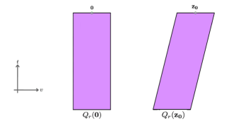
Figure 2. On the left the cylinder ${Q}_{r}({\bf 0})$ centred at the origin; on the right a slanted cylinder ${Q}_{r}(t_{0},x_{0},v_{0})$ according to the invariant transformation given in (2.3).

This is a nontrivial result (​​[37, Theorem 1.3]), but the exponent $0<\beta<1$ in the estimate above is in fact a root, and thus a strong Harnack inequality cannot be deduced. Also, the cylinders $\widetilde{Q}^{\pm}$ in (1.4) – which are naturally slanted in order to deal with the underlying kinetic geometry – are not the expected ones because there is a substantial gap in time which seems to be related to the not optimal expansion of positiveness in the proofs there (see in particular Figure 2 in [37]); compare in fact with the slanted cylinders in [43, 32, 34] as well as with the sharp ones in our forthcoming Theorems 1.2 and 1.3 here, also pictured in forthcoming Figure 1. Again, for integro-differential equations, the situation is different than for classical second order equations. For this, we take the liberty to quote the clarifying explanation by the authors in [32, Pag. 548], «It is not true that the maximum of a nonnegative subsolution can be bounded above by a multiple of its $L^{2}$ norm. One needs to impose an extra global restriction (in this case we assume $0\leq f\leq 1$ globally). This is because of nonlocal effects, since the positive values of the function outside the domain of the equation may pull the maximum upwards.»

In order to overcome the nonlocality issues mentioned above which will also prevent an almost direct strong Harnack inequality from Hölder estimates, in the present paper we found a way to present a totally new $\delta$-interpolation $L^{\infty}$-inequality with tail for weak subsolutions to (1.1) which are not required to being nonnegative. The parameter $0<\delta\leq 1$ in such a boundedness estimate can suitably chosen in order to balance in a quantitative way the local contributions and the nonlocal ones; see in particular in the right-side of the inequality (1.5) in the theorem below the nonlocal kinetic tail ${\rm Tail}_{p}$ quantity, for which we immediately refer to forthcoming Definition 2.1 in Section 2.2 where one can find also related observations on the fractional framework and the underlying hypoelliptic geometry. We are ready to state the aforementioned local boundedness result. We have the following

Theorem 1.1 ($\delta$-interpolative $L^{\infty}$-$L^{2}$ estimate).

For any $s\in(0,1)$, let $f\in\mathcal{W}$ be a weak subsolution to (1.1) in $\varOmega$ and let ${{Q}_{1}\equiv{Q}_{1}({\bf 0})}\subset\varOmega$. Then, for any $Q_{\frac{r}{2}}\equiv Q_{\frac{r}{2}}({\bf 0})$, any $\delta\in(0,1]$, and any $p>p^{\star}$, it holds

(1.5) $$\sup_{Q_{\frac{r}{2}}}f\leq c\,(\delta r^{4s})^{-\frac{1}{2\varepsilon_{*}}}\big{(}\int_{{Q}_{r}}f_{+}^{2}\,{\rm d}v\,{\rm d}x\,{\rm d}t\big{)}^{\frac{1}{2}}+\delta{\rm Tail}_{p}(f_{+};{\bf 0},r,r/2)\,,$$

where ${Q}_{r}:=(-r^{2s},0]\times B_{r^{1+2s}}\times B_{r}$, and the quantity $\varepsilon_{*}>0$ and $p^{\star}>2$ depend only on the dimension $n$ and the exponent $s$, whereas the positive constant $c$ depends also on the kernel structural constant $\varLambda$ in (2.4).

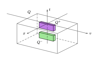
Figure 1. The geometry of the Harnack inequalities for kinetic equations with integro-differential diffusion.

The proof will rely on a precise energy estimate which will essentially involve a Caccioppoli inequality with tail combined with a summability gain result for subsolutions – in turn based on the fundamental solution for the fractional Kolmogorov equation; see forthcoming Lemma 3.1 – as well as with a fine iterative argument taking into account both the ${\rm Tail}_{p}$ term and the desired interpolative effect.

As expected, the result in Theorem 1.1 above will permit us to bypass the aforementioned extra global restriction usually assumed in the previous literature, in turn being fundamental in order to prove the other main results in the present paper. We start with a weak Harnack inequality in the case when the function $f$ is merely a weak supersolution to (1.1).

Theorem 1.2 (The weak Harnack inequality).

For any $s\in(0,1)$, let $f\in\mathcal{W}$ be a nonnegative weak supersolution to (1.1) in $\varOmega$ and let ${Q}_{1}({\bf 0})\equiv{Q}_{1}\subset\varOmega$. Then, there exist $r_{0}$, $c$ and $\zeta$ depending on $s$ and the dimension $n$ such that, for any $0<r<r_{0}$, it holds

(1.6) $$\Big{(}\,\mathchoice{\mathop{\kern 1.99997pt\vrule width=6.00006pt,height=3.0pt,depth=-2.49997pt\kern-8.00003pt\intop}\nolimits_{\kern-2.79996pt{Q}_{r}^{-}}}{\mathop{\kern 1.00006pt\vrule width=5.0pt,height=3.0pt,depth=-2.59996pt\kern-6.00006pt\intop}\nolimits_{{Q}_{r}^{-}}}{\mathop{\kern 1.00006pt\vrule width=5.0pt,height=3.0pt,depth=-2.59996pt\kern-6.00006pt\intop}\nolimits_{{Q}_{r}^{-}}}{\mathop{\kern 1.00006pt\vrule width=5.0pt,height=3.0pt,depth=-2.59996pt\kern-6.00006pt\intop}\nolimits_{{Q}_{r}^{-}}}f(t,x,v)^{\zeta}\,{\rm d}v\,{\rm d}x\,{\rm d}t\,\Big{)}^{\frac{1}{\zeta}}\,\leq\,c\inf_{{Q}_{r}^{+}}f\,\,,$$

where

(1.7) $${Q}_{r}^{+}:=(-r^{2s},0]\times B_{r^{1+2s}}\times B_{r}\quad\text{and}\quad{Q}_{r}^{-}:=(-1,-1+r^{2s}]\times B_{r^{1+2s}}\times B_{r}.$$

The proof of Theorem 1.2 will be finalized by extending the De Giorgi approach; that is, by proving both a new suitable Intermediate Value lemma and a Measure-to-Pointwise lemma. This is in the same spirit of the pioneering work [8], as well as of recent parabolic results for fractional heat equations (as seen, e. g., in [44, 35]. See, also, [9] for related regularity estimates for the fractional parabolic obstacle problem). However, because of the difficulties naturally arising in the hypoelliptic framework here, we have to deal with the intrinsic peculiarities following by the natural scalings trichotomy: time, space and velocity. In addition, since we are seeking for clean Harnack inequalities on optimal (local ) slanted cylinders with no gap in time, we will handle all the related nonlocal estimates in a possibly sharp way by taking into account the tail contributions in this sort of expansion of positivity of suitable subsolutions. The $\delta$-interpolative $L^{\infty}$-$L^{2}$ inequality in Theorem 1.1 will be in fact applied to a suitable (not positive) sequence $g=g_{k}$ approximating an auxiliary subsolutions to (1.1) which is built starting from the supersolutions $f$. Also, whereas we have to operate several modifications in usual fractional estimates, we still cannot apply the standard Krylov-Safonov covering lemma in the framework we are dealing with. For these reasons, we eventually complete the proof of Theorem 1.2 thanks to an applications of the new Ink-spots Theorem by Imbert and Silvestre in [32, Section 9] which will allow us to deal with the naturally slanted kinetic cylinders; see Section 2.1 below.

Finally, still without requiring no additional boundedness assumptions for solutions $f$ to (1.1), we are able to prove the very first strong Harnack inequality for kinetic equations with nonlocal diffusion in velocity. Our main result reads as follows,

Theorem 1.3 (The Harnack inequality).

For any $s\in(0,1)$, let $f\in\mathcal{W}$ be a nonnegative weak solution to (1.1) in $\varOmega$ and let ${Q}_{1}({\bf 0})\equiv{Q}_{1}\subset\varOmega$. Then, there exist $r_{0}$, and $c$ depending on $s$ and the dimension $n$ such that, for any $0<r<r_{0}$, it holds

(1.8) $$\sup\limits_{{Q}^{-}_{r}}f\,\leq\,c\,\inf\limits_{{Q}^{+}_{r}}f\,,$$

where the slanted cylinders ${Q}^{\pm}$ are those defined in (1.7).

The proof will follow by combining all the previous results, together with a precise control of the Tail of the solution in accord with the summability exponent $p^{\star}$ in Theorem 1.1; see the beginning of Section 7. In this respect, it is worth mentioning that our approach steps outside from the nonlocal parabolic counterpart where one can usually take care of the nonlocality by a sort of time slicing via a supremum tail. Here, since a $(t,x)$-freezing is basically not admissible because of the transport term in the very form of the kinetic equation in (1.1), we introduced and made use of the integral  $\operatorname*{{\rm Tail}}_{p}$ quantity.

We then will combine the weak Harnack inequality (1.6) in Theorem 1.2 with an application of the local boundedness inequality in (1.5) by suitably choosing the interpolation parameter $\delta$ there. A new iterative argument taking into account the involved transport and diffusion radii is finally applied in order to complete the estimate in (1.8). This will rely on a new Besicovitch’s covering lemma for slanted cylinders; see forthcoming Lemma 6.1 at Page 6.1, which reminds to the classical covering argument appearing in the last step of most regularity results for both local and/or nonlocal elliptic or parabolic problems via the usual variational approach. We believe that the latter is a very general argument that will have to be taken into account in other results and extensions in the kinetic frameworks.

All in all, let us summarize the contributions of the present paper. We prove the validity of the very first strong Harnack inequality for a class of nonlocal kinetic equations, whose diffusion term in velocity is given by fractional Laplacian-type operators with measurable coefficients, in turn extending to the nonlocal framework Harnack inequalities for the classical Kolmogorov-Fokker-Planck equation, as, e. ​g., in [22], as well as extending to the kinetic framework Harnack inequalities for both the fractional elliptic and parabolic equation (​​[25, 44]). Also, thanks to our strategy, no a priori boundedness is assumed on the solutions, which in fact is proven even for subsolutions without sign assumptions, via the introduction of an integral kinetic tail and suitable energy estimates. As a further addition, both our strategy and proofs are feasible to be used in very general hypoelliptic framework, and our final new slanted covering Lemma is basically untied to our equation (1.1) being in fact a purely geometric property and the kinetic counterpart of classical Besicovitch covering-type results.

1.1. Further developments

We would believe our whole approach and new general independent results to be the veritable starting point in order to attack several open problems related to nonlocal kinetic equations, as, e. g., those listed below.

$\bullet$ By replacing the linear diffusion class of fractional operators with nonlinear $p$-Laplacian-type operators, as for instance in [35, 36]. The nonlinear growth $p$ framework in those Gagliardo seminorms seems to be not so far from the framework presented here in the superquadratic case when $p>2$; the singular case when $1<p<2$ being trickier. However, several “linear” fractional techniques are not disposable; it is no accident that Harnack inequalities are still not available even in the space homogeneous counterpart; say, in the parabolic setting. Nevertheless, our estimates – and the techniques employed in order to treat nonlinear fractional parabolic equations [35] – might be a first outset for dealing with the fractional counterpart of nonlinear subelliptic operators.

$\bullet$ Coming back to purely kinetic equations, our strategy and techniques could be repeated in order to attack the very wide class of integro-differential kernels as those considered in [32, 39], and thus implying a strong Harnack-type inequality for the Boltzmann non-cutoff equation. Such a result appears to be challenging, because of the weaker assumptions on the involved kernels in the diffusion term still enjoying some subtle cancellation property, but lacking a pointwise control as in the purely fractional framework. However, by essentially following our strategy one can take advantage of the fact that a sharp weak Harnack inequality (Theorem 1.6 in [32]) and several other important estimates are already available; see [32, 33, 39]. Lastly, our Besicovitch covering result will be finally applied with no modifications at all.

$\bullet$ Our result in Theorem 1.3 could be of some feasibility even to apparently unrelated problems, as, a concrete example, in the mean fields game theory. It is known that under specific assumptions, mean field games can be seen as a coupled system of two equations, a Fokker-Planck-type equation evolving forward in time (governing the evolution of the density function of the agents), and a Hamilton-Jacobi-type equation evolving backward in time (governing the computation of the optimal path for the agents). Such a forward vs. backward propagation in time should lead to interesting phenomena in time which are present in nature but they have not been investigated in the nonlocal framework yet. Our contribution in the present manuscript together with other recent results and new techniques as the ones developed in [13, 21, 12] could be unexpectedly helpful for such an intricate investigation.

$\bullet$ Finally, it is well known about the many direct consequences and applications of a strong Harnack inequality, as for instance, maximum principles, eigenvalues estimates, Liouville-type theorems, comparison principles, global integrability, and so on.

1.2. The paper is organized as follows

In Section 2 below we fix the notation by also introducing the fractional kinetic framework. In Section 3 we prove fundamental kinetic energy estimates which tail and our $\delta$-interpolative $L^{\infty}$-$L^{2}$ estimate in Theorem (1.1). Section 4 is devoted to a nonlocal expansion of positivity (via De Giorgi-type intermediate lemma and measure-to-pointwise lemma) in order to accurately estimate the infimum of the subsolutions to (1.1), which precisely takes into account the nonlocality in the diffusion via the kinetic tail ${\rm Tail}_{p}$. In Section 5 we shall complete the proof of Theorem 1.2, and in subsequent Section 6 we state and prove the new Besicovitch-type covering result which naturally can be applied in general kinetic geometries. Finally, in Section 7 we are able to prove the strong Harnack inequality given by Theorem 1.3.

2. Preliminaries

In this section we fix notation, and we briefly recall the necessary underlying framework in which one needs to work in order to deal with the class of nonlocal kinetic equations as in (1.1). For a more comprehensive analysis of Lie groups in the kinetic setting we refer the reader to the surveys [3, 2] and the references therein; the interested reader could also refer to the recent paper [38] which deals with the class of operators in (1.2) by presenting an intrinsic Taylor formula in our framework.

2.1. The underlying geometry

We start by endowing $\mathds{R}^{1+2n}=\mathds{R}\times\mathds{R}^{n}\times\mathds{R}^{n}$ of the group law $\circ$ given by

(2.1) $$(t,x,v)\circ(t_{0},x_{0},v_{0}):=\big{(}t+t_{0},\,x+x_{0}+tv_{0},\,v+v_{0}\big{)},$$

so that $(\mathds{R}^{1+2n},\,\circ)$ is a Lie group with identity element ${\bf 0}\equiv(0,0,0)$ and inverse element for $(t,x,v)\in\mathds{R}^{1+2n}$ given by $(-t,\,-x+tv,\,-v)$.

For any $r>0$, consider the usual anisotropic dilation $\delta_{r}:\mathds{R}^{1+2n}\mapsto\mathds{R}^{1+2n}$ defined by

(2.2) $$\delta_{r}(t,x,v):=\big{(}r^{2s}t,\,r^{1+2s}x,\,rv\big{)},$$

so that if $u$ is a solution to (1.1), then the function $u_{r}=u_{r}(t,x,v)$ such that

$$u_{r}(t,x,v):=u\left(r^{2s}t,\,r^{1+2s}x,\,rv\right)$$

does satisfy the same equation in a suitably rescaled domain.

As customary in the hypoelliptic setting, we need to introduce a family of fractional kinetic cylinders respecting the invariant transformations defined above. For every $(t_{0},x_{0},v_{0})\in\mathds{R}^{1+2n}$ and for every $r>0$, the slanted cylinder ${Q}_{r}={Q}_{r}(t_{0},x_{0},v_{0})$ is defined as follows,

(2.3) $${Q}_{r}(t_{0},x_{0},v_{0})\!\!\! := \!\!\!(t_{0},x_{0},v_{0})\,\circ\,\delta_{r}\big{(}(-1,0]\times B_{1}\times B_{1}\big{)}$$

$$\equiv \!\!\!\Big{\{}(t,x,v)\in\mathds{R}^{1+2n}:\,t_{0}-r^{2s}<t\leq t_{0},$$

$$\qquad\qquad\qquad\quad\ \left|(x-x_{0})-(t-t_{0})v_{0}\right|<r^{1+2s},\ \lvert v-v_{0}\rvert<r\Big{\}}.$$

In order to simplify the notation, we denote by ${Q}_{r}$ a cylinder centred in $(0,0,0)$ of radius $r$; that is,

$${Q}_{r}\equiv{Q}_{r}({\bf 0}):=U_{r}(0,0)\times B_{r}(0)=(-r^{2s},0]\times B_{r^{1+2s}}(0)\times B_{r}(0)\,.$$

Now, we recall a suitable covering argument in the same flavour of the Krylov-Safonov Ink-spots theorem. Indeed, in our framework one cannot plainly apply the usual Calderón-Zygmund decomposition, because there is no space to tile slanted cylinders with varying slopes. This is a major difficulty in the nonlocal kinetic framework which has been firstly addressed in an original way by Imbert and Silvestre in [32], who were able to state and prove a custom version of the ink-spots theorem. Such a result, that we will present right below in Theorem 2.1, will allow us to conclude the proof of the weak Harnack inequality. Instead, for what concerns the strong Harnack inequality in (1.8), as mentioned in the Introduction, we will state and prove a new Besicovitch-type covering, which is also suitable for very general kinetic-type frameworks when slanted cylinders do naturally lead the involved geometry; see forthcoming Section 6. In order to state Imbert-Silvestre’s Ink-Spots Theorem, we need to introduce the stacked (and slanted ) cylinders $\bar{{Q}}^{m}_{r}$ for some given $m\in\mathds{N}$. We have

$$\bar{{Q}}^{m}_{r}(t_{0},x_{0},v_{0})\!\!\!\! :=\!\!\!\! \Big{\{}(t,x,v)\in\mathds{R}^{1+2n}:\,0<t-t_{0}\leq mr^{2s},$$

$$\qquad\quad\quad\left|(x-x_{0})-(t-t_{0})v_{0}\right|<(m+2)r^{1+2s},\ \lvert v-v_{0}\rvert<r\Big{\}}.$$

Notice that the cylinder $\bar{{Q}}_{r}^{m}$ starts at the end (in time) of ${Q}_{r}$ and its duration (still in time) is exactly $m$-times the one of ${Q}_{r}$, whereas its spatial radius is $m+2$-times the one of ${Q}_{r}$; see Figure 3 below.

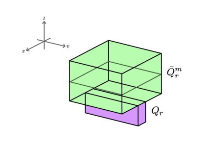
Figure 3. A stacked (and slanted) cylinder $\bar{{Q}}_{r}^{m}$. We refer to Section 10 in [32] for a very detailed analysis and further related results.

Then we have the following

Theorem 2.1 (the Ink-spots Theorem with leakage; see [32, Corollary 10.2]).

Let $E\subset F$ be bounded measurable sets. Assume that for some constant $\mu\in(0,1)$,

• $E\subset{Q}_{1}$,

• if a cylinder ${Q}\subset{Q}_{1}$ satisfies $|{Q}\cap E|\geq(1-\mu)|{Q}|$, then $\bar{{Q}}^{m}\subset F$ and also ${Q}={Q}_{\sigma}(t_{0},x_{0},v_{0})$ for some $\sigma\in(0,r_{0})$.

Then,

$$|E|\,\leq\,\frac{m+1}{m}(1-c\mu)\left(|F\cap{Q}_{1}|+Cmr_{0}^{2s}\right)\\$$

for some constants $c$ and $C$ depending only on $n$ and $s$.

It is worth noticing that related Krylov-Safonov-type results both in the local and nonlocal kinetic framework can be also found in [40, 41]. We would also mention that it was used in [1] for dealing with solutions to a class of Kolmogorov-Fokker-Planck equations in non-divergence form.

2.2. The nonlocal energy setting

We now introduce our fractional functional setting. Let $\varOmega_{v}$ be an open subset of $\mathds{R}^{n}$; for $s\in(0,1)$ recall the definition of the classical fractional Sobolev spaces $H^{s}(\varOmega_{v})$; i. ​e.,

$$H^{s}(\varOmega_{v})\equiv W^{s,2}(\varOmega_{v}):=\left\{f\in L^{2}(\varOmega_{v})\;:\;\left[f\right]_{H^{s}(\varOmega_{v})}<+\infty\right\}\,,$$

where the fractional seminorm $\left[f\right]_{H^{s}(\varOmega_{v})}$ is the usual one via Gagliardo kernels,

$$\left[f\right]_{H^{s}(\varOmega_{v})}:=\left(\int_{\varOmega_{v}}\int_{\varOmega_{v}}\frac{\lvert f(v)-f(w)\rvert^{2}}{\lvert v-w\rvert^{n+2s}}\,\,{\rm d}v\,{\rm d}w\right)^{1/2}.$$

A norm of $H^{s}(\varOmega_{v})$ is given by

$${\left\|f\right\|}_{H^{s}(\varOmega_{v})}:={\left\|f\right\|}_{L^{2}(\varOmega_{v})}+\left[f\right]_{H^{s}(\varOmega_{v})}.$$

A function $f$ belongs to $H_{\rm\operatorname{loc}}^{s}(\varOmega_{v})$ if $f\in H^{s}(\varOmega_{v}^{\prime})$ whenever $\varOmega_{v}^{\prime}\Subset\varOmega_{v}$.

As mentioned in the Introduction, the kernel $K:\mathds{R}^{n}\times\mathds{R}^{n}\to[0,\infty)$ is a measurable kernel having $s$-differentiability for any $s\in(0,1)$; that is, there exists a positive constant $\varLambda$ such that

(2.4) $$\varLambda^{-1}|v-w|^{-n-2s}\leq\,K(v,w)\,\leq\varLambda|v-w|^{-n-2s},\quad\text{for a.~{}\!e.}\ v,w\in\mathds{R}^{n},$$

though most of the estimates in the rest of the paper will still work by weakening such a pointwise control from above, by assuming appropriate coercivity, local integral boundedness and cancelation properties. The pointwise control from below by a Gagliardo-type kernel, on the contrary, is strongly used in some of the needed estimates. However, for the sake of simplicity, we prefer to present our results for the class of measurable kernel as in (2.4), so that the reader has just to keep in mind the case when the diffusion in velocity is a purely fractional Laplacian with coefficients. Consequently, no precise dependance on the constant $\varLambda$ will be explicitly written when not needed.

As expected when dealing with nonlocal operators, the long-range contributions must be taken into account.

Definition 2.1 (The kinetic nonlocal tail).

Let $(t_{0},x_{0},v_{0})\in\varOmega:=(t_{1},t_{2})\times\varOmega_{x}\times\varOmega_{v}\subset\mathds{R}^{1+2n}$ and $R>0$ be such that $U_{R}(t_{0},x_{0})\subset(t_{1},t_{2})\times\varOmega_{x}$, and let $f$ be a measurable function on $(t_{1},t_{2})\times\varOmega_{x}\times\mathds{R}^{n}$. For any $p\in[1,\infty]$ the “kinetic nonlocal tail of $f$ centred in $(t_{0},x_{0},v_{0})$ of transport radius $R$ and diffusion radius $r$” is the quantity  ${\rm Tail}_{p}\equiv{\rm Tail}_{p}(f;(t_{0},x_{0},v_{0}),R,r)$ given by

$${\rm Tail}_{p}(f;(t_{0},x_{0},v_{0}),R,r)$$

(2.5) $$\qquad\quad:=\Big{[}\int_{U_{R}(t_{0},x_{0})}\big{(}\int_{\mathds{R}^{n}\setminus B_{r}(v_{0})}\frac{\lvert f(t,x,v)\rvert}{\lvert v_{0}-v\rvert^{n+2s}}\,{\rm d}v\big{)}^{p}\,{\rm d}x\,{\rm d}t\Big{]}^{\frac{1}{p}}.$$

Despite being not needed in the present manuscript, it is worth mentioning that in the case when $p=\infty$ the kinetic tail definition is meant to be given by taking the $L^{\infty}$-norm in $(t,x)$ instead of the $L^{p}$ one in (2.1).

The kinetic nonlocal tail reminds of the nonlocal tail quantity firstly defined in the purely $p$-fractional elliptic setting in [15, 16] and subsequently proven to be decisive in the analysis of many other nonlocal problems when a fine quantitative control of the naturally arising long-range interactions is needed; see, e. ​g. [31, 6, 44, 35, 7] and the references therein. Several tail related properties of nonlocal harmonic functions are naturally expected – as for instance the fact that their tail is finite, and that their tail is controlled by that of their negative part, and so on – and they are proven in [30]. However, their kinetic counterparts are not for free, and we need to operate step by step in the forthcoming proofs here; see for instance the precise estimates in the proof of the $\delta$-interpolative $L^{\infty}$ inequality and in the control Lemma 7.1 in the final section.

It is also worth noticing that it is usually the nonnegativeness of solutions to interfere with the validity of Harnack inequalities in fractional settings, and Tail$((f)_{-})$ is the decisive player in such a game, as it has been firstly showed by Kaßmann in [24, 25] and then confirmed in the many subsequently related results. On the contrary, our strategy to make use of a nonlocal $L^{\infty}$-$L^{2}$-type estimate does involve an auxiliary (possibly not positive) subsolution $g$ whose error term will be controlled by the kinetic nonlocal tail of its positive part $(g)_{+}$; see the formulation in (1.5) and the details in the related proofs in the rest of the present paper.

Given $\varOmega:=(t_{1},t_{2})\times\varOmega_{x}\times\varOmega_{v}\subset\mathds{R}^{1+2n}$ we denote by $\mathcal{W}$ the natural functions space where weak solutions to (1.1) are taken. We have

(2.6) $$\mathcal{W}:=\Big{\{}f\in L^{2}\big{(}(t_{1},t_{2})\times\varOmega_{x};\,H^{s}(\mathds{R}^{n})\big{)}\\ :\left[\partial_{t}+v\cdot\nabla_{x}\right]f\in L^{2}\big{(}(t_{1},t_{2})\times\varOmega_{x};\,H^{-s}(\mathds{R}^{n})\big{)}\Big{\}}.$$

Furthermore, we denote by $\mathcal{E}(\cdot)$ the nonlocal energy associated with our diffusion term $\mathcal{L}_{v}$ in (1.3)

$$\begin{split}&\mathcal{E}(f(t,x,\cdot),\phi(t,x,\cdot))\\[2.15277pt] &\qquad\quad:=\int_{\mathds{R}^{n}}\int_{\mathds{R}^{n}}\big{(}f(t,x,v)-f(t,x,w)\big{)}\big{(}\phi(t,x,v)-\phi(t,x,w)\big{)}K(v,w)\,\,{\rm d}v\,{\rm d}w\,,\end{split}$$

for any test function $\phi$ smooth enough. We are now in the position to recall the definition of weak sub- and supersolution.

Definition 2.2.

A function $f\in\mathcal{W}$ is a  weak subsolution (resp., supersolution) to (1.1) in $\varOmega$ if

$$\displaystyle\int_{t_{1}}^{t_{2}}\int_{\varOmega_{x}}\mathcal{E}\left(f(t,x,\cdot),\phi(t,x,\cdot)\right)\,\,{\rm d}x\,{\rm d}t$$

$$\qquad\qquad\qquad+\,\int_{t_{1}}^{t_{2}}\int_{\varOmega_{x}}\langle(\partial_{t}f+v\cdot\nabla_{x}f)\,|\,\phi\rangle\,{\rm d}x\,{\rm d}t\,\leq\,0\ \ \big{(}\geq\,0,\,\text{resp.}\big{)},$$

for any nonnegative $\phi\in\mathcal{W}$ such that ${\rm supp}\,\phi\Subset\varOmega$; in the display above we denote by $\langle\cdot\,|\,\cdot\rangle$ the usual duality paring between $H^{s}(\mathds{R}^{n})$ and $H^{-s}(\mathds{R}^{n})$.
A function $f\in\mathcal{W}$ is a weak solution to (1.1) if it is both a weak sub- and supersolution.

3. Interpolative $L^{\infty}$-$L^{2}$-type estimate

This section is devoted to the proof of the local boundedness estimate with tail for subsolutions to (1.1) with no a priori sign assumptions, as stated in Theorem 1.1.

3.1. Kinetic Energy estimates with tail

Firstly, we need a precise energy estimate which will require to prove a Caccioppoli-type estimate with (kinetic) tail, and a Gehring-type one for subsolutions to (1.1). We have the following

Lemma 3.1 (Gain of integrability for subsolutions).

Let $f$ be a weak subsolution in $\varOmega$ according to Definition​ 2.2 and let ${{Q}_{1}\equiv{Q}_{1}({\bf 0})}\subset\varOmega$. For any $Q_{r}\equiv Q_{r}({\bf 0})\subset Q_{1}$, any $q\in[2,q^{\star})$, where $q^{\star}=q^{\star}(n,s)>2$, and any $\varrho<r$, the following estimate does hold,

(3.1) $$\|\omega\|^{2}_{L^{q}(Q_{\varrho})}\!\! \leq \!\!c\int_{U_{r}}\int_{\mathds{R}^{n}}\int_{\mathds{R}^{n}}\frac{\omega(v)\omega(w)\lvert\varphi(v)-\varphi(w)\rvert^{2}}{\lvert v-w\rvert^{n+2s}}\,{\rm d}v\,{\rm d}w\,{\rm d}x\,{\rm d}t$$

$$\!\!+\,c\int_{{Q}_{r}}({|v\cdot\nabla_{x}(\varphi^{2})|+|v\cdot\nabla_{x}\varphi|^{2}})\omega^{2}\,{\rm d}v\,{\rm d}x\,{\rm d}t+c\,r^{2s}\int_{{Q}_{r}}(\omega\varphi)^{2}\,{\rm d}v\,{\rm d}x\,{\rm d}t\,.$$

where $\omega:=(f-k)_{+}$, for any $k\in\mathds{R}$, and where $\varphi=\varphi(x,v)$ is a cut-off function such that $\varphi(x,v)\equiv 1$ in $B_{\varrho^{1+2s}}\times B_{\varrho}$ and $\varphi\equiv 0$ outside $B_{r^{1+2s}}\times B_{r}$.

Proof..

For the sake of the reader, it is convenient to divide the present proof in two separate steps.

Step 1: Kinetic Caccioppoli inequality with tail

Up to regularizing by mollification, for any fixed $t\in(-r^{2s},0]$ we can assume that $\omega\varphi^{2}$ is sufficiently regular in order to be an admissible test function compactly supported in the cylinder $({Q}_{r})^{t}:=\{(v,x)\in~{}\mathds{R}^{2n}:(t,x,v)\in~{}{Q}_{r}\}$. Consider now the weak formulation in Definition 2.2 by choosing as a test function $\phi\equiv\omega\varphi^{2}$ there; for a. ​e. $t\in(-{r^{2s}},0]$ it yields

(3.2) $$0\ \geq \ \int_{({Q}_{r})^{t}}(\partial_{t}f+v\cdot\nabla_{x}f)\omega\varphi^{2}\,{\rm d}x\,{\rm d}v$$

$$\ +\int_{B_{r^{1+2s}}}\mathcal{E}(f,\omega\varphi^{2})\,{\rm d}x\,=:\,I_{1}+I_{2}.$$

We start by considering $I_{1}$. Using the fact that $\partial_{t}\varphi=0$, we have that

(3.3) $$I_{1}\ \geq\ \frac{1}{2}\frac{\,{\rm d}}{\,{\rm d}t}\int_{({Q}_{r})^{t}}(\omega\varphi)^{2}\,{\rm d}x\,{\rm d}v\\ -\frac{1}{2}\int_{({Q}_{r})^{t}}|v\cdot\nabla_{x}(\varphi^{2})|\omega^{2}\,{\rm d}x\,{\rm d}v\,.$$

For what concern $I_{2}$ we note that

$$\big{(}f(v)-f(w)\big{)}\big{(}\omega\varphi^{2}(v)-\omega\varphi^{2}(w)\big{)}$$

$$\qquad\qquad\qquad\qquad=\ \big{(}(f(v)-k)-(f(w)-k)\big{)}\big{(}\omega\varphi^{2}(v)-\omega\varphi^{2}(w)\big{)}$$

$$\qquad\qquad\qquad\qquad\geq\ \big{(}\omega\varphi(v)-\omega\varphi(w)\big{)}^{2}-\omega(v)\omega(w)\lvert\varphi(v)-\varphi(w)\rvert^{2}\,,$$

which yields

$$I_{2} \geq \int_{B_{r^{1+2s}}}[\omega\varphi]^{2}_{H^{s}(\mathds{R}^{n})}\,{\rm d}x$$

$$-\int_{B_{r^{1+2s}}}\int_{\mathds{R}^{n}}\int_{\mathds{R}^{n}}\frac{\omega(v)\omega(w)\lvert\varphi(v)-\varphi(w)\rvert^{2}}{\lvert v-w\rvert^{n+2s}}\,{\rm d}v\,{\rm d}w\,{\rm d}x\,,$$

where we also used the definition of the kernel $K$ in (2.4) by neglecting a constant depending on $\varLambda$ there, for the sake of simplicity. Combining (3.3) and (3.1) with (3.2), it yields

$$\frac{1}{2}\frac{\,{\rm d}}{\,{\rm d}t}\int_{({Q}_{r})^{t}}(\omega\varphi)^{2}\,{\rm d}x\,{\rm d}v+\int_{B_{r^{1+2s}}}[\omega\varphi]^{2}_{H^{s}(\mathds{R}^{n})}\,{\rm d}x$$

(3.5) $$\qquad\qquad\quad\leq c\int_{B_{r^{1+2s}}}\int_{\mathds{R}^{n}}\int_{\mathds{R}^{n}}\frac{\omega(v)\omega(w)\lvert\varphi(v)-\varphi(w)\rvert^{2}}{\lvert v-w\rvert^{n+2s}}\,{\rm d}v\,{\rm d}w\,{\rm d}x$$

$$\qquad\qquad\qquad+c\int_{({Q}_{r})^{t}}|v\cdot\nabla_{x}(\varphi^{2})|\omega^{2}\,{\rm d}v\,{\rm d}x\,,$$

Then, by integrating (3.1) in $[\tau_{1},\tau_{2}]$, for $-r^{2s}\leq\tau_{1}<\tau_{2}\leq 0$, we get

$$\int_{B_{r^{1+2s}}\times B_{r}}(\omega\varphi)^{2}(\tau_{2},x,v)\,{\rm d}x\,{\rm d}v+\int_{\tau_{1}}^{\tau_{2}}\int_{B_{r^{1+2s}}}[\omega\varphi]^{2}_{H^{s}(\mathds{R}^{n})}\,{\rm d}x\,{\rm d}t$$

(3.6) $$\qquad\qquad\leq c\int_{U_{r}}\int_{\mathds{R}^{n}}\int_{\mathds{R}^{n}}\frac{\omega(v)\omega(w)\lvert\varphi(v)-\varphi(w)\rvert^{2}}{\lvert v-w\rvert^{n+2s}}\,{\rm d}v\,{\rm d}w\,{\rm d}x\,{\rm d}t$$

$$\qquad\qquad\quad+\,c\int_{{Q}_{r}}|v\cdot\nabla_{x}(\varphi^{2})|\omega^{2}\,{\rm d}v\,{\rm d}x\,{\rm d}t+c\int_{B_{r^{1+2s}}\times B_{r}}(\omega\varphi)^{2}(\tau_{1},x,v)\,{\rm d}x\,{\rm d}v\,.$$

Taking the supremum over $\tau_{2}$ on the left-hand side and the average integral over $\tau_{1}\in[-r^{2s},0]$ on both sides of the inequality, we get

$$\sup_{t\in[-r^{2s},0]}\int_{B_{r^{1+2s}}\times B_{r}}(\omega\varphi)^{2}\,{\rm d}v\,{\rm d}x$$

(3.7) $$\qquad\qquad\quad\leq c\int_{U_{r}}\int_{\mathds{R}^{n}}\int_{\mathds{R}^{n}}\frac{\omega(v)\omega(w)\lvert\varphi(v)-\varphi(w)\rvert^{2}}{\lvert v-w\rvert^{n+2s}}\,{\rm d}v\,{\rm d}w\,{\rm d}x\,{\rm d}t$$

$$\qquad\qquad\qquad+\,c\int_{{Q}_{r}}|v\cdot\nabla_{x}(\varphi^{2})|\,\omega^{2}\,{\rm d}v\,{\rm d}x\,{\rm d}t+c\,r^{2s}\int_{{Q}_{r}}(\omega\varphi)^{2}\,{\rm d}v\,{\rm d}x\,{\rm d}t\,.$$

Reconsidering (3.1) and evaluating with $\tau_{1}=-r^{2s}$ and $\tau_{2}=0$ there, we then have

$$\int_{U_{r}}[\omega\varphi]^{2}_{H^{s}(\mathds{R}^{n})}\,{\rm d}x\,{\rm d}t$$

$$\qquad\leq c\int_{U_{r}}\int_{\mathds{R}^{n}}\int_{\mathds{R}^{n}}\frac{\omega(v)\omega(w)\lvert\varphi(v)-\varphi(w)\rvert^{2}}{\lvert v-w\rvert^{n+2s}}\,{\rm d}v\,{\rm d}w\,{\rm d}x\,{\rm d}t$$

$$\qquad\quad+\,c\int_{{Q}_{r}}|v\cdot\nabla_{x}(\varphi^{2})|\omega^{2}\,{\rm d}v\,{\rm d}x\,{\rm d}t+c\,r^{2s}\int_{{Q}_{r}}(\omega\varphi)^{2}\,{\rm d}v\,{\rm d}x\,{\rm d}t$$

Thus, combining the display above with (3.1), we obtain the following Caccioppoli-type estimate,

$$\sup_{t\in[-r^{2s},0]}\int_{B_{r^{1+2s}}\times B_{r}}(\omega\varphi)^{2}\,{\rm d}v\,{\rm d}x+\int_{U_{r}}[\omega\varphi]^{2}_{H^{s}(\mathds{R}^{n})}\,{\rm d}x\,{\rm d}t$$

(3.8) $$\qquad\quad\leq c\int_{U_{r}}\int_{\mathds{R}^{n}}\int_{\mathds{R}^{n}}\frac{\omega(v)\omega(w)\lvert\varphi(v)-\varphi(w)\rvert^{2}}{\lvert v-w\rvert^{n+2s}}\,{\rm d}v\,{\rm d}w\,{\rm d}x\,{\rm d}t$$

$$\qquad\qquad+\,c\int_{{Q}_{r}}\,|v\cdot\nabla_{x}(\varphi)^{2}|\omega^{2}\,{\rm d}v\,{\rm d}x\,{\rm d}t+cr^{2s}\int_{{Q}_{r}}(\omega\varphi)^{2}\,{\rm d}v\,{\rm d}x\,{\rm d}t\,.$$

Step 2: Local $L^{q}$-estimate for subsolutions

Now, an $L^{q}$-estimate whose proof is in the same spirit of the original result for solutions to the Boltzmann equation without cut-off by Imbert and Silvestre – see in particular Lemma 6.1 and Proposition 2.2 in [32] – which in turn reminds to the strategy in [40] and to classical Gehring-type results; see in particular Sections 2 and 3 there. Nevertheless, for the sake of the reader, we sketch the proof below.

Furthermore, it is worth noticing that the exponent $p^{\star}$ in  the statement of Theorem 1.1 will basically show up here, being linked to the maximal gain in summability in forthcoming formula (3.9).

Consider the smooth function $\varphi=\varphi(x,v)$ such that $\varphi(x,v)\equiv 1$ in $B_{\varrho^{1+2s}}\times B_{\varrho}$ and $\varphi\equiv 0$ outside $B_{r^{1+2s}}\times B_{r}$, with $\varrho<r<1$.

Then, the function $g:=\omega\varphi$ satisfies the following

$$[\partial_{t}+v\cdot\nabla_{x}]~{}g-\mathcal{L}_{v}g\,\leq\,{\left([\partial_{t}+v\cdot\nabla_{x}]\omega\right)\varphi}+\omega\left([\partial_{t}+v\cdot\nabla_{x}]\varphi\right)-\varLambda^{-1}(-\varDelta_{v})^{s}g\,;$$

where $\varLambda$ is the kernel structural constant in (2.4). Now, we can apply the result in Lemma 6.1 in[32] – by taking $H_{2}:=\varLambda^{-1}(-\varDelta_{v})^{\frac{s}{2}}g$ and $H_{1}:={\left([\partial_{t}+v\cdot\nabla_{x}]\omega\right)\varphi}+\omega\left([\partial_{t}+v\cdot\nabla_{x}]\varphi\right)$ there – and we get that, for any $q\geq 2$ such that $q<{q^{\star}}$ with

(3.9) $$q^{\star}:=\displaystyle 2+\frac{2s}{n(1+s)}\,,$$

the following estimate holds,

$$\|g\|_{L^{q}([-r^{2s},0]\times\mathds{R}^{2n})}$$

$$\quad\leq c\Big{(}\|g(-r^{2s},\cdot,\cdot)\|_{L^{2}(\mathds{R}^{2n})}+{\|([\partial_{t}+v\cdot\nabla_{x}]\omega)\varphi\|_{L^{2}([-r^{2s},0]\times\mathds{R}^{2n})}}$$

$$\qquad+\|\omega([\partial_{t}+v\cdot\nabla_{x}]\varphi)\|_{L^{2}([-r^{2s},0]\times\mathds{R}^{2n})}+\int_{U_{r}}[g]^{2}_{H^{s}(\mathds{R}^{n})}\,{\rm d}x\,{\rm d}t\Big{)}$$

$$\quad\leq c\left(\|g(-r^{2s},\cdot,\cdot)\|_{L^{2}(\mathds{R}^{2n})}+\|\omega(v\cdot\nabla_{x}\varphi)\|_{L^{2}([-r^{2s},0]\times\mathds{R}^{2n})}+\,\int_{U_{r}}[g]^{2}_{H^{s}(\mathds{R}^{n})}\,{\rm d}x\,{\rm d}t\right)\,,$$

where we have integrated by parts in the second integral and the positive constant $c$ also depends on $n$ and $s$; recall Proposition 3.6 in [17].

Now, by recalling the definition of $\varphi$, we restate the latter estimate as follows,

$$\|\omega\|_{L^{q}(Q_{\varrho})} \leq c\,\|\omega\varphi(-r^{2s},\cdot,\cdot)\|_{L^{2}(B_{r^{1+2s}}\times B_{r})}$$

$$+c\ \|\omega(v\cdot\nabla_{x}\varphi)\|_{L^{2}(Q_{r})}+c\int_{U_{r}}[\omega\varphi]^{2}_{H^{s}(\mathds{R}^{n})}\,{\rm d}x\,{\rm d}t\,.$$

Conclusion

It finally suffice to combine (3.1) with (3.1). ∎

We are now in the position to prove the $\delta$-interpolative $L^{\infty}$-$L^{2}$ inequality.

Proof of Theorem 1.1..

Let $r>0$ and, for any $j\in\mathds{N}$, define a decreasing family of positive radii $r_{j}:=\frac{1}{2}(1+2^{-j})r$ and a family of slanted cylinders $Q_{j}\equiv Q_{r_{j}}({\bf 0})$ such that $Q_{j+1}\Subset Q_{j}$ for every $j\in\mathds{N}$. We will denote with $U_{j}:=(-r_{j}^{2s},0]\times B_{r_{j}^{1+2s}}$, so that $Q_{j}:=U_{j}\times B_{r_{j}}$.

Consider a family $\{\varphi_{j}\}_{j\in\mathds{N}}$ of test functions $\varphi_{j}\equiv\varphi_{j}(x,v)\in C^{\infty}_{0}(B_{r_{j}^{1+2s}}\times B_{{r}_{j}})$, such that $0\leq\varphi_{j}\leq 1$, $\varphi_{j}\equiv 1\,\text{on}~{}B_{r_{j+1}^{1+2s}}\times B_{r_{j+1}}$, $\varphi_{j}(x,\cdot)=0$ outside $B_{(r_{j}+r_{j+1})/{2}}$, ${|\nabla_{v}\varphi_{j}|\leq c2^{j+2}/r}$, and ${|v\cdot\nabla_{x}\varphi_{j}|\leq c2^{(j+1)(1+2s)}/r^{2s}}$. For any $j\in\mathds{N}$, let $k_{j}:=(1-2^{-j})k_{0}$, with ${k}_{0}>0$ which will be fixed later on, and define $\omega_{j}:=(f-k_{j})_{+}$.

An application of Lemma 3.1 yields, for some $q\equiv q(n,s)>2$ that

$$\int_{Q_{j+1}}\omega_{j+1}^{2}\,{\rm d}v\,{\rm d}x\,{\rm d}t$$

$$\quad\leq\left(\int_{Q_{j+1}}\omega_{j+1}^{q}\,{\rm d}v\,{\rm d}x\,{\rm d}t\right)^{\frac{2}{q}}|Q_{j+1}\cap\{f\geq k_{j+1}\}|^{1-\frac{2}{q}}\,$$

$$\quad\leq c\left(\int_{U_{j}}\int_{\mathds{R}^{n}}\int_{\mathds{R}^{n}}\frac{\omega_{j+1}(v)\omega_{j+1}(w)\lvert\varphi_{j}(v)-\varphi_{j}(w)\rvert^{2}}{\lvert v-w\rvert^{n+2s}}\,{\rm d}v\,{\rm d}w\,{\rm d}x\,{\rm d}t\right.$$

$$\qquad\left.+\,\int_{{Q}_{j}}({|v\cdot\nabla_{x}(\varphi_{j}^{2})|+|v\cdot\nabla_{x}\varphi_{j}|^{2}})\,\omega_{j+1}^{2}\,{\rm d}v\,{\rm d}x\,{\rm d}t+\,r_{j}^{2s}\int_{{Q}_{j}}(\omega_{j+1}\varphi_{j})^{2}\,{\rm d}v\,{\rm d}x\,{\rm d}t\right)$$

$$\qquad\ \times\,|Q_{j+1}\cap\{f\geq k_{j+1}\}|^{1-\frac{2}{q}}$$

(3.11) $$\qquad\quad\ =:\,(I_{1}+I_{2}+I_{3})|Q_{j+1}\cap\{f\geq k_{j+1}\}|^{1-\frac{2}{q}}$$

We estimate separately the last three integrals. Starting from $I_{1}$, we get that

(3.12) $$I_{1} = c\int_{Q_{j}}\int_{B_{j}}\frac{\omega_{j+1}(v)\omega_{j+1}(w)\lvert\varphi_{j}(v)-\varphi_{j}(w)\rvert^{2}}{\lvert v-w\rvert^{n+2s}}\,{\rm d}v\,{\rm d}w\,{\rm d}x\,{\rm d}t$$

$$+\,c\int_{Q_{j}}\int_{\mathds{R}^{n}\setminus B_{j}}\frac{\omega_{j+1}(v)\omega_{j+1}(w)\varphi_{j}^{2}(v)}{\lvert v-w\rvert^{n+2s}}\,{\rm d}w\,{\rm d}v\,{\rm d}x\,{\rm d}t$$

$$=: I_{1,1}+I_{1,2}\,.$$

The first integral $I_{1,1}$ can be treated assuming $\omega_{j+1}(v)\geq\omega_{j+1}(w)$, noticing that the reverse inequality holds true when one exchanges the roles of $v$ and $w$, as follows,

$$\begin{split}I_{1,2}&\leq\,c{2^{2(j+2)}r^{-2}}\int_{Q_{j}}\omega_{j+1}^{2}\left(\int_{2B_{j}(v)}\frac{\,{\rm d}w}{\lvert v-w\rvert^{n-2(1-s)}}\right)\,{\rm d}v\,{\rm d}x\,{\rm d}t\\[4.30554pt] &\leq\,c{2^{2(j+2)}r^{-2}}\int_{Q_{j}}\omega_{j+1}^{2}\left(\int_{0}^{2r}\varrho^{2(1-s)-1}\,{\rm d}\varrho\right)\,{\rm d}v\,{\rm d}x\,{\rm d}t\\[4.30554pt] &\leq\,\frac{c{2^{2(j+2)}}}{2(1-s){r^{2s}}}\int_{Q_{j}}\omega_{j}^{2}\,{\rm d}v\,{\rm d}x\,{\rm d}t\,.\end{split}$$

As for the second integral $I_{1,2}$, we have by Hölder’s Inequality for some $p>2$ that

$$\begin{split}I_{1,2}&\leq c\int_{Q_{j}\cap\,\text{supp}~{}\varphi_{j}}\int_{\mathds{R}^{n}\setminus B_{j}}\frac{\omega_{j+1}(v)\omega_{j+1}(w)}{\lvert v-w\rvert^{n+2s}}\,{\rm d}w\,{\rm d}v\,{\rm d}x\,{\rm d}t\\[2.15277pt] &\leq\left(\int_{Q_{j}}\omega_{j+1}^{2}\,{\rm d}v\,{\rm d}x\,{\rm d}t\right)^{\frac{1}{2}}\\[2.15277pt] &\quad\times\Big{[}\int_{Q_{j}\cap\,\text{supp}~{}\varphi_{j}}\left(\int_{\mathds{R}^{n}\setminus B_{j}}\frac{\omega_{j+1}(w)}{\lvert v-w\rvert^{n+2s}}\,{\rm d}w\right)^{2}\chi_{\{f(v)>k_{j+1}\}}\,{\rm d}v\,{\rm d}x\,{\rm d}t\Big{]}^{\frac{1}{2}}\\[2.15277pt] &\leq c2^{j(n+2s)}\left(\int_{Q_{j}}\omega_{j}^{2}\,{\rm d}v\,{\rm d}x\,{\rm d}t\right)^{\frac{1}{2}}{\rm Tail}_{p}(f_{+};{\bf 0},r,r/2)\lvert Q_{j}\cap\{f>k_{j+1}\}\rvert^{1-\frac{2}{p}}\\[2.15277pt] &\leq\frac{c2^{j(n+2s+\frac{2p-4}{p})}k_{0}^{2}}{\delta}\left(\int_{Q_{j}}\frac{\omega_{j}^{2}}{k_{0}^{2}}\,{\rm d}v\,{\rm d}x\,{\rm d}t\right)^{\frac{3p-4}{2p}}\,,\end{split}$$

up to choosing

(3.13) $$k_{0}\geq\delta{\rm Tail}_{p}(f_{+};{\bf 0},r,r/2)\qquad\text{for}~{}\delta\in(0,1]\,,$$

and where we have used that, for $w\in\mathds{R}^{n}\setminus B_{j}$ and $v\in\text{supp}~{}\varphi_{j}$ (recalling that the support in the $v$-variable of $\varphi_{j}$ is contained in $B_{(r_{j}+r_{j+1})/{2}}$)

$$\frac{|w|}{|v-w|}\leq 1+\frac{|v|}{|w|-|v|}\leq 1+\frac{r_{j}+r_{j+1}}{r_{j}-r_{j+1}}\leq 2^{j+4}\,.$$

as well as

$$\begin{split}|Q_{j}\cap\{f>k_{j+1}\}|&=|Q_{j}\cap\{f-k_{j}>k_{j+1}-k_{j}\}|\\[3.87495pt] &\leq|Q_{j}\cap\{f-k_{j}>2^{-j-1}k_{0}\}|\\[3.01385pt] &\leq 2^{2j+2}\int_{Q_{j}}\frac{\omega_{j}^{2}}{k_{0}^{2}}\,{\rm d}v\,{\rm d}x\,{\rm d}t\,.\end{split}$$

Combining all the previous estimate for $I_{1,1}$ and $I_{1,2}$ together we get that

(3.14) $$I_{1}\leq\frac{c2^{j(n+2s+\frac{2p-4}{p}{+2})}k_{0}^{2}}{\delta{r^{2s}}}\left[\int_{Q_{j}}\frac{\omega_{j}^{2}}{k_{0}^{2}}\,{\rm d}v\,{\rm d}x\,{\rm d}t+\left(\int_{Q_{j}}\frac{\omega_{j}^{2}}{k_{0}^{2}}\,{\rm d}v\,{\rm d}x\,{\rm d}t\right)^{\frac{3p-4}{2p}}\right]\,.$$

In a similar way, recalling the particular choice of the test function $\varphi_{j}$, we have that

(3.15) $$I_{2}+I_{3} \leq {\frac{c2^{2j(1+2s)}}{r^{4s}}}\int_{Q_{j}}\omega_{j}^{2}\,{\rm d}v\,{\rm d}x\,{\rm d}t$$

$$\leq {\frac{c2^{2j(1+2s)}}{r^{4s}}}\int_{Q_{j}}\omega_{j}^{2}\,{\rm d}v\,{\rm d}x\,{\rm d}t={\frac{c2^{2j(1+2s)}k_{0}^{2}}{r^{4s}}}\int_{Q_{j}}\frac{\omega_{j}^{2}}{k_{0}^{2}}\,{\rm d}v\,{\rm d}x\,{\rm d}t\,.$$

where we have used the fact that

$$|v\cdot\nabla_{x}(\varphi_{j}^{2})|+|v\cdot\nabla_{x}\varphi_{j}|^{2} = 2|\varphi_{j}||v\cdot\nabla_{x}\varphi_{j}|+|v\cdot\nabla_{x}\varphi_{j}|^{2}$$

$$\leq \frac{c2^{j(1+2s)}}{r^{2s}}+\frac{c2^{2j(1+2s)}}{r^{4s}}\leq\frac{c2^{2j(1+2s)}}{r^{4s}}\,,$$

recalling that $r<1$.

Moreover, the measure of the superlevel set in (3.1) can be estimated as follows,

(3.16) $$|Q_{j+1}\cap\{f>k_{j+1}\}|^{1-\frac{2}{q}} = |Q_{j+1}\cap\{f-k_{j}>k_{j+1}-k_{j}\}|^{1-\frac{2}{q}}$$

$$\leq |Q_{j}\cap\{f-k_{j}>2^{-j-1}k_{0}\}|^{1-\frac{2}{q}}$$

$$\leq 2^{j\frac{2q-4}{q}}\left(\int_{Q_{j}}\frac{\omega_{j}^{2}}{k_{0}^{2}}\,{\rm d}v\,{\rm d}x\,{\rm d}t\right)^{1-\frac{2}{q}}\,.$$

We now define $A_{j}$

$$A_{j}:=\int_{Q_{j}}\frac{\omega_{j}^{2}}{k_{0}^{2}}\,\,{\rm d}v\,{\rm d}x\,{\rm d}t\,,$$

so that, by putting (3.14), (3.15) and (3.16) in (3.1), we get

(3.17) $$A_{j+1}\,\leq\,\frac{c2^{j(n+2s+\frac{2p-4}{2p}+{2}+{2(1+2s)}+\frac{2q-4}{q})}}{\delta{r^{4s}}}\left(A_{j}^{1+\frac{q-2}{q}}+A_{j}^{1+\frac{3p-4}{2p}-\frac{2}{q}}\right).$$

Now, note that $1-{2}/{q}>0$, given that $q>2$, and that $\frac{3p-4}{2p}-\frac{2}{q}>0$, which is in fact possible for $p$ large enough, say $p>p^{\star}=p^{\star}(n,s)$, where clearly the latter depends on the growth power $q^{\star}$ defined in (3.9).

Thus, we can rewrite the inequality in (3.17) as follows,

$$A_{j+1}\,\leq\,\frac{cb^{j}}{\delta{r^{4s}}}A_{j}^{1+\varepsilon_{*}}\,,$$

for some $\varepsilon_{*}\equiv\varepsilon_{*}(n,s)$ and $b>1$. Then, up to choosing

$$k_{0}:=(\delta{r^{4s}})^{-\frac{1}{2\varepsilon_{*}}}c^{\frac{1}{2\varepsilon_{*}}}b^{\frac{1}{2\varepsilon_{*}^{2}}}\left(\int_{{Q}_{r}}f_{+}^{2}\,{\rm d}v\,{\rm d}x\,{\rm d}t\right)^{\!\frac{1}{2}}+\delta\,{\rm Tail}_{p}(f_{+};{\bf 0},r,r/2)\,,$$

which is in clear accordance with (3.13). A standard iteration argument yields that $A_{j}\to 0$ as $j\to\infty$, which finally gives the desired result. ∎

4. Towards a Harnack inequality: De Giorgi’s Intermediate Lemma and the Measure-to-pointwise Lemma

This section is devoted to the proof of the main ingredients required to obtain Harnack inequalities in (1.6) and (1.8); i. ​e., the De Giorgi Intermediate Values lemma and the Measure-to-pointwise one, which in turn does also rely on a suitable application of the $\delta$-interpolative $L^{\infty}$ inequality in Theorem 1.1 by carefully estimating the tail contributions; see forthcoming Section 4.2.

4.1. De Giorgi’s Intermediate Values Lemma

Our strategy will extend that in the pioneering paper [8], which will help in some of the estimates on the nonlocal energy terms arising from the diffusion in velocity. However, some decisive modifications need to be carried out because of our kinetic framework; that is, the novel presence of the transport term in (1.1). Also, it is worth noticing that our methods are feasible of further generalizations when more spatial commutators are involved.

Consider $\mu<1$, $r_{3}>r_{2}>0$ and a cut-off function $\varphi\equiv\varphi(x)\in C^{\infty}_{0}(\mathds{R}^{n})$ such that $0\leq\varphi\leq 1$, $\varphi\equiv 1$ in $B_{r_{2}^{1+2s}}$ and $\varphi\equiv 0$ outside $B_{r_{3}^{1+2s}}$. Then define the following three auxiliary functions $F_{i}=F_{i}(v)$,

$$F_{0}(v):=\frac{1}{r_{3}}\max\left\{-r_{3},\,\frac{\min\left\{0,\,|v|^{2}-2r_{3}^{2}\right\}}{r_{3}}\right\}\,,$$

(4.1) $$F_{1}(v):=\frac{1}{r_{3}}\max\left\{-r_{3},\,\frac{\min\left\{0,\,\lvert v\rvert^{2}-r_{3}^{2}\right\}}{r_{3}}\right\}\,,$$

$$F_{2}(v):=\frac{1}{r_{2}}\max\left\{-r_{2},\,\frac{\min\left\{0,\,\lvert v\rvert^{2}-r_{2}^{2}\right\}}{r_{2}}\right\}\,.$$

The underling kinetic geometry is coming up; compare indeed with the single Lipschitz function $F$ which does the job in the purely fractional parabolic setting in [8, Section 4]. Accordingly, we would need the three following consecutive functions $\varphi_{i}$ depending on $F_{i}$,

(4.2) $$\varphi_{i}=\varphi_{i}(x,v):=2-\varphi(x)+\mu^{i}F_{i}(v)\,,\quad\ \text{for}\ i=0,1,2.$$

We can state the following

Theorem 4.1 (De Giorgi’s Intermediate Values Lemma).

Let $f$ be a weak subsolution to (1.1) in $\varOmega$ according to Definition​ 2.2 such that $f\leq 1$ and let ${{Q}_{1}\equiv{Q}_{1}({\bf 0})}\subset\varOmega$. Consider $0<r_{1},r_{2}<r_{3}<{1}$ and $0>t_{2}>t_{1}>-1$. Define now

$${Q}^{(1)}:=(-{1},t_{1}]\times B_{r_{1}^{1+2s}}\times B_{r_{1}},\qquad{Q}^{(2)}:=(t_{2},0]\times B_{r_{2}^{1+2s}}\times B_{r_{2}}$$

$${Q}^{(3)}:=(-{1},0]\times B_{r_{3}^{1+2s}}\times B_{r_{3}}.$$

Given $\delta_{1},\delta_{2}\in(0,1)$ there exist $\nu,\mu\equiv\nu,\mu(\delta_{1},\delta_{2},r_{1},r_{2},r_{3},s,n)$ such that if it holds

(4.3) $$\lvert\{f\leq\varphi_{0}\}\cap{Q}^{(1)}\rvert\geq\delta_{1}\lvert{Q}^{(1)}\rvert\quad\text{and}\quad\lvert\{f\geq\varphi_{2}\}\cap{Q}^{(2)}\rvert\geq\delta_{2}\lvert{Q}^{(2)}\rvert\,,$$

then $f$ satisfies

(4.4) $$\lvert\{\varphi_{0}<f<\varphi_{2}\}\cap{Q}^{(3)}\rvert\geq\nu\lvert{Q}^{(3)}\rvert\,,$$

where $\varphi_{i}$ are defined in (4.2) for $i=1,2,3$.

Proof..

The proof requires a sort of both nonlocal and kinetic approach based on suitable choices also in order to estimate all the energy contributions by tracking explicit dependencies on the involved quantities so that the forthcoming Harnack inequalities will not depend on the local slanted cylinders. We divide it into three steps.

Step 1: The energy estimate

Up to regularizing by mollification, for any fixed $t\in(-1,0]$ we can assume that $(f-\varphi_{1})_{+}$ is sufficiently regular in order to be an admissible test function compactly supported in the cylinder $({Q}^{(3)})^{t}:=\{(v,x)\in~{}\mathds{R}^{2n}:(t,x,v)\in~{}{Q}^{(3)}\}$. Consider now the weak formulation in Definition 2.2 by choosing as a test function $\phi\equiv(f-\varphi_{1})_{+}\eta^{2}$ there, with $\eta\in C^{\infty}_{0}(B_{{(2r_{3})}^{1+2s}})$ be a cut-off function so that $0\leq\eta\leq 1$ and $\eta\equiv 1$ on $B_{r_{2}^{1+2s}}$; for a. ​e. $t\in(-{1},0]$ it yields

(4.5) $$\begin{split}0\ &\geq\ \int_{({Q}^{(3)})^{t}}(\partial_{t}f+v\cdot\nabla_{x}f)(f-\varphi_{1})_{+}\eta^{2}\,{\rm d}x\,{\rm d}v\\[4.30554pt] &\quad\ +\int_{B_{r_{3}^{1+2s}}}\mathcal{E}\big{(}f,(f-\varphi_{1})_{+}\eta^{2}\big{)}\,{\rm d}x\,=:\,I_{1}+I_{2}.\end{split}$$

We start by considering $I_{1}$. Using the fact that $\partial_{t}\varphi_{1}=0$ and that $\nabla_{x}\varphi_{1}\neq 0$ only on $B_{r_{3}^{1+2s}}\setminus B_{r_{2}^{1+2s}}$, we have that

$$I_{1} = \frac{1}{2}\frac{\,{\rm d}}{\,{\rm d}t}\int_{({Q}^{(3)})^{t}}\big{(}(f-\varphi_{1})_{+}\eta\big{)}^{2}\,{\rm d}x\,{\rm d}v$$

$$\quad-\frac{1}{2}\int_{({Q}^{(3)})^{t}}v\cdot\nabla_{x}(\eta^{2})(f-\varphi_{1})_{+}^{2}\,{\rm d}x\,{\rm d}v$$

$$\quad+\int_{({Q}^{(3)})^{t}}v\cdot\nabla_{x}\varphi_{1}(f-\varphi_{1})_{+}\,{\rm d}x\,{\rm d}v$$

$$\geq \frac{1}{2}\min\limits_{B_{r_{3}^{1+2s}}}(\eta^{2})\frac{\,{\rm d}}{\,{\rm d}t}\int_{({Q}^{(3)})^{t}}(f-\varphi_{1})_{+}^{2}\,{\rm d}x\,{\rm d}v$$

$$\quad-\frac{|Q_{1}|(2\|v\cdot\nabla_{x}(\varphi_{1})\|_{L^{\infty}}-\|v\cdot\nabla_{x}(\eta^{2})\|_{L^{\infty}})}{2}\mu^{2}\,,$$

where we have used the fact that $(f-\varphi_{1})_{+}\leq\mu$. Moreover, choosing a proper cut-off function $\eta$ in order to control the second term in the right-hand side of (4.1), we get

(4.7) $$I_{1}\,\gtrsim\,\frac{\,{\rm d}}{\,{\rm d}t}\int_{({Q}^{(3)})^{t}}\big{(}(f-\varphi_{1})_{+}\eta\big{)}^{2}\,{\rm d}x\,{\rm d}v-\mu^{2}\,.$$

We now consider the integral $I_{2}$. We start noticing that by the linearity of the involved energy $\mathcal{E}(\cdot)$, we have that

$$\mathcal{E}(f,(f-\varphi_{1})_{+})$$

(4.8) $$\qquad\qquad=[(f-\varphi_{1})_{+}]_{H^{s}}^{2}-\mathcal{E}((f-\varphi_{1})_{-},(f-\varphi_{1})_{+})+\mathcal{E}(\varphi_{1},(f-\varphi_{1})_{+}).$$

Moreover, we note that

(4.9) $$\mathcal{E}(\varphi_{1},(f-\varphi_{1})_{+}) \leq \frac{1}{2}[(f-\varphi_{1})_{+}]_{H^{s}}^{2}$$

$$+\,2\mu^{2}\int_{\mathds{R}^{n}}\int_{\mathds{R}^{n}}\frac{\lvert F_{1}(v)-F_{1}(w)\rvert^{2}}{\lvert v-w\rvert^{n+2s}}(\chi_{B_{r_{3}}}(v)+\chi_{B_{r_{3}}}(w))\,{\rm d}v\,{\rm d}w$$

$$\leq \frac{1}{2}[(f-\varphi_{1})_{+}]_{H^{s}}^{2}+c\,\mu^{2}\iint_{B_{r_{3}}\times B_{r_{3}}}\frac{\,{\rm d}v\,{\rm d}w}{\lvert v-w\rvert^{n-2(1-s)}}$$

$$\leq \frac{1}{2}[(f-\varphi_{1})_{+}]_{H^{s}}^{2}+c\,\mu^{2}\iint_{B_{r_{3}}\times B_{2r_{3}}(v)}\frac{\,{\rm d}v\,{\rm d}w}{\lvert v-w\rvert^{n-2(1-s)}}$$

$$\leq \frac{1}{2}[(f-\varphi_{1})_{+}]_{H^{s}}^{2}+c\mu^{2}\,,$$

where we have used the Lipschitz continuity of $F_{1}$ – recall its definition in (4.1) – alongside with the definition of $\mathcal{E}$.

Recalling (4.7) and the fact that $-I_{1}\geq I_{2}$ by (4.5), it yields

(4.10) $$c\mu^{2}\geq I_{2}+\frac{\,{\rm d}}{\,{\rm d}t}\int_{({Q}^{(3)})^{t}}(f-\varphi_{1})_{+}^{2}\,{\rm d}x\,{\rm d}v.$$

Moreover, by combining (4.1) with (4.9), we obtain that

(4.11) $$\begin{split}I_{2}\ &\leq\ \frac{3}{2}\int_{B_{r_{3}^{1+2s}}}[(f-\varphi_{1})_{+}]_{H^{s}}^{2}\eta^{2}\,{\rm d}x\\[2.15277pt] &\quad-\int_{B_{r_{3}^{1+2s}}}\mathcal{E}((f-\varphi_{1})_{-},(f-\varphi_{1})_{+})\eta^{2}\,{\rm d}x+c\,\mu^{2}.\end{split}$$

Then, by summing (4.11) with (4.10), and recalling that $\mu<1$, it follows

$$\begin{split}c\mu^{2}-2I_{2}\,&\geq\,\frac{\,{\rm d}}{\,{\rm d}t}\int_{({Q}^{(3)})^{t}}(f-\varphi_{1})_{+}^{2}\,{\rm d}x\,{\rm d}v\\[2.15277pt] &\quad-\frac{3}{2}\int_{B_{r_{3}^{1+2s}}}[(f-\varphi_{1})_{+}]_{H^{s}}^{2}\eta^{2}\,{\rm d}x\\[2.15277pt] &\quad+\int_{B_{r_{3}^{1+2s}}}\mathcal{E}((f-\varphi_{1})_{-},(f-\varphi_{1})_{+})\eta^{2}\,{\rm d}x\,;\end{split}$$

so that, also in view of (4.1), we finally arrive at

$$\begin{split}c\mu^{2}\,&\geq\,\frac{\,{\rm d}}{\,{\rm d}t}\int_{({Q}^{(3)})^{t}}(f-\varphi_{1})_{+}^{2}\,{\rm d}x\,{\rm d}v\\[2.15277pt] &\quad+\frac{1}{2}\int_{B_{r_{3}^{1+2s}}}[(f-\varphi_{1})_{+}]_{H^{s}}^{2}\eta^{2}\,{\rm d}x-\int_{B_{r_{3}^{1+2s}}}\mathcal{E}((f-\varphi_{1})_{-},(f-\varphi_{1})_{+})\eta^{2}\,{\rm d}x\\[2.15277pt] &\quad+2\int_{B_{r_{3}^{1+2s}}}\mathcal{E}(\varphi_{1},(f-\varphi_{1})_{+})\eta^{2}\,{\rm d}x.\end{split}$$

We now estimate the energy contribution $\mathcal{E}(\varphi_{1},(f-\varphi_{1})_{+})$. We firstly split the contribution given by the nonlocal term as follows,

$$\mathcal{E}(\varphi_{1},(f-\varphi_{1})_{+})$$

(4.12) $$\ \qquad=\iint_{\lvert v-w\rvert\geq 1}\frac{\big{(}\varphi_{1}(v)-\varphi_{1}(w)\big{)}\big{(}(f-\varphi_{1})_{+}(v)-(f-\varphi_{1})_{+}(w)\big{)}}{\lvert v-w\rvert^{n+2s}}\,{\rm d}v\,{\rm d}w$$

$$\ \quad\qquad+\iint_{\lvert v-w\rvert<1}\frac{\big{(}\varphi_{1}(v)-\varphi_{1}(w)\big{)}\big{(}(f-\varphi_{1})_{+}(v)-(f-\varphi_{1})_{+}(w)\big{)}}{\lvert v-w\rvert^{n+2s}}\,{\rm d}v\,{\rm d}w.$$

Using the very definition of $\varphi_{1}$ and the boundedness of the auxiliary function $F_{1}$ in (4.1), we obtain that

$$\left|\iint_{\lvert v-w\rvert\geq 1}\frac{(\varphi_{1}(v)-\varphi_{1}(w))(f-\varphi_{1})_{+}(v)}{\lvert v-w\rvert^{n+2s}}\,{\rm d}v\,{\rm d}w\right|$$

$$\qquad\qquad\leq c\mu\,\int_{\lvert v-w\rvert\geq 1}\frac{\,{\rm d}w}{\lvert v-w\rvert^{n+2s}}\,\int_{\mathds{R}^{n}}(f-\varphi_{1})_{+}(v)\,{\rm d}v$$

$$\qquad\qquad\leq c\,\mu^{2}\int_{1}^{\infty}\sigma^{-1-2s}\,{\rm d}\sigma\ =\ c\,\mu^{2}\,,$$

where we have also used that $(f-\varphi_{1})_{+}\leq\mu$ and it is compactly supported. Then, the first integral in the right-hand side of (4.1) can be estimated as follows

$$\left|\iint_{\lvert v-w\rvert\geq 1}\frac{(\varphi_{1}(v)-\varphi_{1}(w))((f-\varphi_{1})_{+}(v)-(f-\varphi_{1})_{+}(w))}{\lvert v-w\rvert^{n+2s}}\,{\rm d}v\,{\rm d}w\right|\,\leq\,c\,\mu^{2}.$$

Let us consider now the second integral in the right-hand side of (4.1). By suitable applying the Hölder inequality and the Young inequality, we can deduce that

$$\left|\iint_{\lvert v-w\rvert<1}\frac{(\varphi_{1}(v)-\varphi_{1}(w))((f-\varphi_{1})_{+}(v)-(f-\varphi_{1})_{+}(w))}{\lvert v-w\rvert^{n+2s}}\,{\rm d}v\,{\rm d}w\right|$$

$$\qquad\qquad\qquad\qquad\leq\varepsilon\iint_{\lvert v-w\rvert<1}\frac{|(f-\varphi_{1})_{+}(v)-(f-\varphi_{1})_{+}(w)|^{2}}{\lvert v-w\rvert^{n+2s}}\,{\rm d}v\,{\rm d}w$$

$$\qquad\qquad\qquad\qquad\quad+\frac{1}{\varepsilon}\iint_{\lvert v-w\rvert<1}\frac{|\varphi_{1}(v)-\varphi_{1}(w)|^{2}}{\lvert v-w\rvert^{n+2s}}\,{\rm d}v\,{\rm d}w\,,$$

for some $\varepsilon>0$ which will be fixed later on. Now, the second integral in the right-hand side of the display above can be estimated via the definition of $\varphi_{1}$ as well as done in previous estimate (4.11), so that

$$\iint_{\lvert v-w\rvert<1}\frac{|\varphi_{1}(v)-\varphi_{1}(w)|^{2}\,{\rm d}v\,{\rm d}w}{\lvert v-w\rvert^{n+2s}} \leq \mu^{2}\iint_{\lvert v-w\rvert<1}\frac{\lvert F_{1}(v)-F_{1}(w)\rvert^{2}}{\lvert v-w\rvert^{n+2s}}\chi_{B_{r_{3}}}(v)\,{\rm d}v\,{\rm d}w$$

$$\leq \mu^{2}\int_{B_{r_{3}}}\int_{\lvert v-w\rvert<1}\frac{\,{\rm d}w}{\lvert v-w\rvert^{n-2(1-s)}}\,{\rm d}v$$

$$\leq c\,\mu^{2}\int_{0}^{1}\sigma^{1+2s}\,{\rm d}\sigma\int_{B_{r_{3}}}\,{\rm d}v$$

$$\leq \frac{c\,\mu^{2}\lvert B_{r_{3}}\rvert}{2(1+s)}\,.$$

All in all, from (4.1) the following estimate has been obtained,

$$\left|\mathcal{E}(\varphi_{1},(f-\varphi_{1})_{+})\right|\,\leq\,c(\varepsilon)\,\mu^{2}+\varepsilon\left[(f-\varphi_{1})_{+}\right]^{2}_{H^{s}},$$

for a suitable positive constant $c=c(\varepsilon)$. Choosing $\varepsilon$ sufficiently small in order to absorb the seminorm $\left[(f-\varphi_{1})_{+}\right]_{H^{s}}$ in the right-hand side of the display above, it yields

(4.13) $$\begin{split}c\mu^{2}\,&\geq\,\frac{\,{\rm d}}{\,{\rm d}t}\int_{({Q}^{(3)})^{t}}(f-\varphi_{1})_{+}^{2}\,{\rm d}x\,{\rm d}v\\[2.15277pt] &\quad\ +\int_{B_{r_{3}^{1+2s}}}\left[(f-\varphi_{1})_{+}\right]_{H^{s}}^{2}\eta^{2}\,{\rm d}x\\[2.15277pt] &\quad\ -\int_{B_{r_{3}^{1+2s}}}\mathcal{E}\big{(}(f-\varphi_{1})_{-},(f-\varphi_{1})_{+}\big{)}\eta^{2}\,{\rm d}x.\end{split}$$

Moreover, recalling that $(f-\varphi_{1})_{+}(f-\varphi_{1})_{-}=0$, we obtain that

$$\mathcal{E}((f-\varphi_{1})_{-},(f-\varphi_{1})_{+})=-2\int_{\mathds{R}^{n}}\int_{\mathds{R}^{n}}\frac{(f-\varphi_{1})_{+}(v)(f-\varphi_{1})_{-}(w)}{\lvert v-w\rvert^{n+2s}}\,{\rm d}v\,{\rm d}w.$$

Hence, the inequality in (4.13), also by recalling the fact that $\eta\in C^{\infty}_{0}(B_{(2r_{3})^{1+2s}})$, can be written as follows,

(4.14) $$\begin{split}c\mu^{2}&\,\geq\,\frac{\,{\rm d}}{\,{\rm d}t}\int_{({Q}^{(3)})^{t}}(f-\varphi_{1})_{+}^{2}\,{\rm d}x\,{\rm d}v\\[2.15277pt] &\qquad+\int_{B_{r_{3}^{1+2s}}}\left[(f-\varphi_{1})_{+}\right]_{H^{s}}^{2}\eta^{2}\,{\rm d}x\\[2.15277pt] &\qquad+\int_{B_{r_{3}^{1+2s}}}\int_{\mathds{R}^{n}}\int_{\mathds{R}^{n}}\frac{(f-\varphi_{1})_{+}(v)(f-\varphi_{1})_{-}(w)}{\lvert v-w\rvert^{n+2s}}\,{\rm d}v\,{\rm d}w\,{\rm d}x.\end{split}$$

Notice that both the second and the third term in the inequality above in (4.14) are nonnegative, once we define

(4.15) $$\mathcal{H}(t):=\int_{({Q}^{(3)})^{t}}(f-\varphi_{1})_{+}^{2}(t,x,v)\,{\rm d}x\,{\rm d}v\,,$$

it yields that for $-{1}<t\leq 0$ we have

$$\mathcal{H}^{\prime}(t)\leq c\mu^{2}\,.$$

Moreover, let us note that $(f-\varphi_{1})_{+}\leq\mu\mathds{1}_{{Q}^{(3)}}$, hence $\mathcal{H}(t)\leq c\,\mu^{2}$. Then, integrating inequality (4.14) in time for $-1<\tau_{1}<\tau_{2}\leq 0$, we finally get

$$\displaystyle\int_{\tau_{1}}^{\tau_{2}}\int_{B_{r_{3}^{1+2s}}}\int_{\mathds{R}^{n}}\int_{\mathds{R}^{n}}\frac{(f-\varphi_{1})_{+}(v)(f-\varphi_{1})_{-}(w)}{\lvert v-w\rvert^{n+2s}}\,{\rm d}v\,{\rm d}w\,{\rm d}x\,{\rm d}t$$

$$\hskip 170.71652pt\leq c\,\mu^{2}(\tau_{2}-\tau_{1})+\left|\mathcal{H}(\tau_{2})-\mathcal{H}(\tau_{1})\right|$$

(4.16) $$\hskip 170.71652pt\leq c\,\mu^{2}(\tau_{2}-\tau_{1})+c\,\mu^{2}\ \leq\ c\,\mu^{2}\,.$$

Step 2: Estimating time and space slices

Starting from the assumption in (4.3), let us call $\varSigma$ the set of times in $(-{1},t_{1}]$ defined as follows,

$$\varSigma:=\left\{t\in(-1,t_{1}]\,:\,\left|{\left\{f(t,\cdot,\cdot)\leq\varphi_{0}\right\}\cap({Q}^{(3)})^{t}}\right|\geq\frac{\delta_{1}\lvert{Q}^{(1)}\rvert}{4}\right\}\,.$$

Such a set $\varSigma$ satisfies the following estimate,

$$\left|{\varSigma}\right|\geq\displaystyle\frac{\delta_{1}}{2}{\big{(}\frac{r_{1}}{r_{3}}\big{)}^{2(n+s)}(t_{1}+1)}\,.$$

Indeed, a plain computation leads to

$$\left|\left\{f\leq\varphi_{0}\right\}\cap\left(({Q}^{(3)})^{t}\times(-{1},t_{1}]\right)\right|$$

$$\quad\quad=\,\left|\left\{f(t,\cdot,\cdot)\leq\varphi_{0}\right\}\cap({Q}^{(3)})^{t}\right||\varSigma|\,+\,\left|\left\{f(t,\cdot,\cdot)\leq\varphi_{0}\right\}\cap({Q}^{(3)})^{t}\right|\left|\mathscr{C}_{(-{1},t_{1}]}(\varSigma)\right|,$$

where, as customary, by $\mathscr{C}_{(-1,t_{1}]}(\varSigma)$ we denoted the complementary set of $\varSigma$ in $(-1,t_{1}]$. Thus, we get

$$|\{f(t,\cdot,\cdot)\leq\varphi_{0}\}\cap({Q}^{(3)})^{t}||\varSigma|$$

$$\qquad\qquad\geq\,\lvert\{f\leq\varphi_{0}\}\cap{Q}^{(1)}\rvert-|\{f(t,\cdot,\cdot)\leq\varphi_{0}\}\cap({Q}^{(3)})^{t}||\mathscr{C}_{(-1,t_{1}]}(\varSigma)|$$

$$\qquad\qquad\geq\,\delta_{1}\lvert{Q}^{(1)}\rvert-\frac{\delta_{1}\lvert{Q}^{(1)}\rvert}{4}|\mathscr{C}_{(-{1},t_{1}]}(\varSigma)|$$

$$\qquad\qquad\geq\,\delta_{1}\lvert{Q}^{(1)}\rvert-\frac{\delta_{1}\lvert{Q}^{(1)}\rvert}{4}$$

$$\qquad\qquad\geq\,\frac{3}{4}\delta_{1}\lvert{Q}^{(1)}\rvert\,>\,\frac{1}{2}\delta_{1}\lvert{Q}^{(1)}\rvert\,.$$

Then, dividing the previous inequality on both sides by $|\{f(t,\cdot,\cdot)\leq\varphi_{0}\}\cap({Q}^{(3)})^{t}|$ yields

$$|\varSigma| \geq \frac{\delta_{1}}{2}\frac{\lvert{Q}^{(1)}\rvert}{|\{f(t,\cdot,\cdot)\leq\varphi_{0}\}\cap({Q}^{(3)})^{t}|}$$

$$\geq \frac{\delta_{1}}{2}\frac{\lvert{Q}^{(1)}\rvert}{|{Q}^{(3)}|}\,\geq\,\frac{\delta_{1}}{2}{\big{(}\frac{r_{1}}{r_{3}}\big{)}^{2(n+s)}(t_{1}+1)}\,,$$

as claimed.

Starting again from estimate (4.1), we have

(4.17) $$c\,\mu^{2}\! \geq \!\!\!\!\int_{-1}^{0}\int_{B_{r_{3}^{1+2s}}}\int_{\mathds{R}^{n}}\int_{\mathds{R}^{n}}\frac{(f-\varphi_{1})_{+}(v)(f-\varphi_{1})_{-}(w)}{\lvert v-w\rvert^{n+2s}}\,{\rm d}v\,{\rm d}w\,{\rm d}x\,{\rm d}t$$

$$\geq \!\!\!\!c\int_{\varSigma}\int_{B_{r_{3}^{1+2s}}}\iint_{\mathds{R}^{n}\times B_{r_{3}}}(f-\varphi_{1})_{+}(v)(f-\varphi_{1})_{-}(w)\,{\rm d}v\,{\rm d}w\,{\rm d}x\,{\rm d}t$$

$$\geq \!\!\!\!c\int_{\varSigma}\int_{B_{r_{3}^{1+2s}}}\int_{(\{f(\cdot,x,t)\leq\varphi_{0}\}\cap B_{r_{3}})\times B_{r_{3}}}(f-\varphi_{1})_{+}(v)(\varphi_{1}-\varphi_{0})_{-}(w)\,{\rm d}v\,{\rm d}w\,{\rm d}x\,{\rm d}t$$

$$\geq \!\!\!\!c\int_{\varSigma}\int_{B_{r_{3}^{1+2s}}}\int_{(\{f(\cdot,x,t)\leq\varphi_{0}\}\cap B_{r_{3}})\times B_{r_{3}}}(f-\varphi_{1})_{+}(v)(\mu F_{1}-F_{0})_{+}(w)\,{\rm d}v\,{\rm d}w\,{\rm d}x\,{\rm d}t$$

$$\geq \!\!\!\!c(1-\mu)\int_{\varSigma}\int_{B_{r_{3}^{1+2s}}}\left(\int_{B_{r_{3}}}(f-\varphi_{1})_{+}(v)\,{\rm d}v\right)\left|\left\{f(\cdot,x,t)\leq\varphi_{0}\right\}\cap B_{r_{3}}\right|\,{\rm d}x\,{\rm d}t$$

$$\geq\,\frac{c(1-\mu)|Q^{(1)}|\delta_{1}}{4\mu}\int_{\varSigma}\int_{({Q}^{(3)})^{t}}\left(f-\varphi_{1}\right)_{+}^{2}\,{\rm d}v\,{\rm d}x\,{\rm d}t\,,$$

where we have also used the following estimates,

$$\begin{split}&\left|\left\{f(\cdot,x,t)\leq\varphi_{0}\right\}\cap B_{r_{3}}\right|\,\geq\,\frac{\delta_{1}|Q^{(1)}|}{4}\quad\text{a.~{}\!e. on}~{}B_{r_{3}^{1+2s}}\ \text{and for~{}$t\in\varSigma$}\,,\\[3.87495pt] &(f-\varphi_{1})_{+}\,\leq\,\mu\,,\\[3.87495pt] &(\varphi_{1}-\varphi_{0})_{-}\,=\,(\mu F_{1}-F_{0})_{+}\,\geq\,1-\mu\quad\text{on}~{}B_{r_{3}}\,,\\[3.87495pt] \text{and}\hskip 54.06006pt&\inf_{B_{r_{3}}\times B_{r_{3}}}\lvert v-w\rvert^{-n-2s}\,\geq\,c>0.\end{split}$$

Hence, we eventually get

$$\int_{\varSigma}\int_{({Q}^{(3)})^{t}}(f-\varphi_{1})_{+}^{2}\,{\rm d}v\,{\rm d}x\,{\rm d}t\,\leq\,\frac{c\mu^{3}}{(1-\mu)\delta_{1}}\,\leq\,\mu^{3-1/8}\,,$$

if $\mu$ is sufficiently small. In particular, we have that

(4.18) $$\int_{({Q}^{(3)})^{t}}(f-\varphi_{1})_{+}^{2}\,{\rm d}v\,{\rm d}x\,\leq\,\mu^{{3}-1/4}\,$$

does hold for any $t\in(-{1},t_{1}]$ except on a set $\Upsilon$ for which we have that, by Chebychev’s Inequality,

$$\lvert\Upsilon\rvert := \left|\left\{t\in(-{1},t_{1}]\,:\,\|(f-\varphi_{1})_{+}(t,\cdot)\|_{L^{2}(({Q}^{(3)})^{t})}^{2}>\mu^{3-1/4}\right\}\right|\leq\mu^{1/8}.$$

Taking a smaller $\mu$ such that

(4.19) $$\mu\leq\big{(}\frac{\delta_{1}}{4}\big{)}^{8},$$

we can finally have that (4.18) holds on a set $t\in(-{1},t_{1}]$ of measure greater than $\displaystyle\frac{3}{4}\delta_{1}$.

Step 3: The intermediate set for $f$

Assume now that there exists a time $\tau_{0}\in(t_{2},0)$ such that

$$\lvert\{(v,x)|(f-\varphi_{2})_{+}(\tau_{0},\cdot,\cdot)>0\}\cap{Q}^{(2)}\rvert>\frac{\delta_{2}}{2}\lvert{Q}^{(2)}\rvert.$$

Thus, at time $\tau_{0}$ we have

(4.20) $$\mathcal{H}(\tau_{0}) = \int_{({Q}^{(3)})^{\tau_{0}}}(f-\varphi_{1})_{+}^{2}(v,x,\tau_{0})\,{\rm d}x\,{\rm d}v$$

$$\geq \int_{({Q}^{(3)})^{\tau_{0}}}(\varphi_{2}-\varphi_{1})^{2}(v,x,\tau_{0})\chi_{\{(f-\varphi_{2})_{+}(\cdot,\tau_{0})>0\}}\,{\rm d}x\,{\rm d}v$$

$$\geq \int_{({Q}^{(3)})^{\tau_{0}}}(\mu^{2}F_{2}-\mu F_{1})^{2}(v,x,\tau_{0})\chi_{\{(f-\varphi_{2})_{+}(\cdot,\tau_{0})>0\}}\,{\rm d}x\,{\rm d}v$$

$$\geq \int_{({Q}^{(2)})^{\tau_{0}}}\mu^{2}(\mu F_{2}-F_{1})^{2}(v)\,\chi_{\{(f-\varphi_{2})_{+}(\tau_{0},\cdot,\cdot)>0\}}\,{\rm d}x\,{\rm d}v$$

$$\stackrel{{\scriptstyle\eqref{mu_choice}}}{{\geq}} \frac{\mu^{2}}{2}{\min_{v\in B_{r_{2}}\atop\mu\leq(\frac{\delta_{1}}{4})^{8}}(\mu F_{2}-F_{1})^{2}}\,\left|\left\{(x,v)\,:\,(f-\varphi_{2})_{+}(\tau_{0},\cdot,\cdot)>0\right\}\cap{Q}^{(2)}\right|$$

$$\geq \mathfrak{c}\frac{\mu^{2}}{4}\delta_{2}\lvert{Q}^{(2)}\rvert\,,$$

where the positive constant $\mathfrak{c}$ depends only on $F_{1},F_{2}$ and $\delta_{1}$.

Moreover, consider a time ${\overline{\tau}}\leq\tau_{0}$ such that ${\overline{\tau}}\in(-1,t_{1}]$ such that

$$\mathcal{H}({\overline{\tau}})=\int_{({Q}^{(3)})^{{\overline{\tau}}}}(f-\varphi_{1})^{2}_{+}(v,x,{\overline{\tau}})\,{\rm d}v\,{\rm d}x\,\leq\,\mu^{3-1/4}.$$

In this way, we choose $\mu$ sufficiently small (up to shrinking a smaller $\delta_{2}$ if needed) such that

(4.21) $$\mu^{1-1/4}\geq\mathfrak{c}\frac{\lvert{Q}^{(2)}\rvert\delta_{2}}{16}.$$

and thus the energy $\mathcal{H}(\cdot)$ of $(f-\varphi_{1})_{+}^{2}(t,\cdot,\cdot)$ passes through the range of times

$$D:=\left\{\tau\in({\overline{\tau}},\tau_{0})\,:\,{\mathfrak{c}}\frac{\lvert{Q}^{(2)}\rvert\mu^{2}}{16}\delta_{2}<\mathcal{H}(\tau)<{\mathfrak{c}}\frac{\lvert{Q}^{(2)}\rvert\mu^{2}}{4}\delta_{2}\right\}.$$

In such a range of times we have that

(4.22) $$\left|\left\{(f-\varphi_{2})_{+}(\tau,\cdot,\cdot)>0\right\}\cap({Q}^{(3)})^{\tau}\right|\leq\frac{\delta_{2}}{2}|{Q}^{(2)}|.$$

Indeed, by contradiction assume that the reverse inequality holds true for some $\tau\in D$. Hence, at such a time slice $\tau$, going through the same computation as in (4.20), we will arrive at $\mathcal{H}(\tau)\geq{\mathfrak{c}}\frac{\lvert{Q}^{(2)}\rvert\mu^{2}}{4}\delta_{2}$ which is in contradiction with the fact that $\tau\in D$.

Thus, up to choosing $\delta_{2}$ sufficiently small, we have that the measure of the set appearing in (4.22) is negligible.

Now, we estimate the size of the set $U$ of times slice of $D$ for which

$$\,\,\left|\left\{(f-\varphi_{0})_{+}(\tau,\cdot,\cdot)\leq 0\right\}\cap({Q}^{(3)})^{t}\right|\,\geq\,\delta_{1}|{Q}^{(2)}|.$$

By (4.1) we have

$$c\,\mu^{2} \geq \int_{-{1}}^{0}\int_{B_{r_{3}^{1+2s}}}\int_{\mathds{R}^{n}}\int_{\mathds{R}^{n}}\frac{(f-\varphi_{1})_{+}(v)(f-\varphi_{1})_{-}(w)}{\lvert v-w\rvert^{n+2s}}\,{\rm d}v\,{\rm d}w\,{\rm d}x\,{\rm d}t$$

$$\geq \frac{c\delta_{1}|{Q}^{(2)}|}{\mu}\int_{U}\int_{B_{r_{3}^{1+2s}}}\int_{\mathds{R}^{n}}(f-\varphi_{1})^{2}\,{\rm d}v\,{\rm d}x\,{\rm d}t$$

$$\geq \frac{c\delta_{1}\delta_{2}\lvert U\rvert\mu|{Q}^{(2)}|}{16}\,,$$

where we have followed a similar reasoning as in (4.17)–(4.20), and in the last line we have also used the fact that $\tau\in U\subset D$. Therefore, we obtain that

$$\lvert U\rvert\,\leq\,\frac{c\mu}{\delta_{1}\delta_{2}|{Q}^{(2)}|}.$$

Then, by choosing

(4.23) $$\mu\,\leq\,\delta_{1}\delta_{2}\lvert D\rvert|{Q}^{(2)}|/(2c)$$

we plainly deduce that

$$\lvert U\rvert\,\leq\,\frac{\lvert D\rvert}{2}.$$

Consider now those times $\tau\in D$ which are not in $U$. Hence, we have

(4.24) $$\left|\left\{\varphi_{0}<f(\tau,\cdot,\cdot)<\varphi_{2}\right\}\cap({Q}^{(3)})^{\tau}\right|\geq\frac{\lvert{Q}^{(3)}\rvert}{2}\,,$$

Indeed,

$$\left|\left\{\varphi_{0}<f(\tau,\cdot,\cdot)<\varphi_{2}\right\}\cap({Q}^{(3)})^{\tau}\right|$$

$$\quad\qquad\,\geq\lvert({Q}^{(3)})^{\tau}\rvert-\left|\left\{\varphi_{0}>f(\tau,\cdot,\cdot)\right\}\cap({Q}^{(3)})^{\tau}\right|-\left|\left\{f(\tau,\cdot,\cdot)>\varphi_{2}\right\}\cap({Q}^{(3)})^{\tau}\right|$$

$$\quad\qquad\,\geq|({Q}^{(3)})^{\tau}|-\delta_{1}|{Q}^{(2)}|-\frac{\delta_{2}}{2}\lvert{Q}^{(2)}\rvert$$

$$\quad\qquad\geq\,\frac{\lvert{Q}^{(3)}\rvert}{2}\,,$$

up to choosing $\delta_{1}$ and $\delta_{2}$ small enough.

Hence, by (4.24), we finally deduce

$$\lvert\{\varphi_{0}<f<\varphi_{2}\}\cap{Q}^{(3)}\rvert = \int_{-{1}}^{0}\lvert\{\varphi_{0}<f(\tau,\cdot,\cdot)<\varphi_{2}\}\cap({Q}^{(3)})^{\tau}\rvert\,{\rm d}\tau$$

$$\geq \int_{D\setminus U}\lvert\{\varphi_{0}<f(\tau,\cdot,\cdot)<\varphi_{2}\}\cap({Q}^{(3)})^{\tau}\rvert\,{\rm d}\tau$$

$$\geq {\frac{\lvert D\rvert\lvert{Q}^{(3)}\rvert}{4}}\,\geq\,\nu\lvert{Q}^{(3)}\rvert\,,$$

up to choosing a constant $\nu\equiv\nu(\delta_{1},\delta_{2})$ sufficiently small, as desired. ∎

4.2. The Measure-to-pointwise Lemma

In order to prove a Measure-to-point-wise-type lemma, we will employ Theorem 4.1 established in the previous section, together with the nonlocal $L^{\infty}$-$L^{2}$-type estimate with tail (1.5) stated in the Introduction.

Theorem 4.2 (Measure-to-pointwise Lemma).

Let $\mathring{\delta}\in(0,1)$ and let ${Q}^{(1)},{Q}^{(2)}\subset{Q_{1}({\bf 0})}\subset\varOmega$ be the ones introduced in Theorem 4.1. Let $g$ be a weak subsolution to (1.1) in $\varOmega$ such that $g\leq 1$ in $\varOmega$ and

(4.25) $$|\left\{g\leq 0\right\}\cap{Q}^{(1)}|\geq\mathring{\delta}|{Q}^{(1)}|.$$

Then there exists a real number $\vartheta\equiv\vartheta(\mathring{\delta},\mu,\nu)>0$ such that

(4.26) $$g\leq 1-\vartheta\qquad\text{in }\,\,{Q}_{\varrho},$$

for any $\varrho\in(0,r_{2}/2)$, where $\nu$ and $\mu$ are the constants introduced in Theorem 4.1.

Proof..

Let us consider $0<\mu<1$ as in (4.2) and let us define a sequence of functions

$$g_{k}:=\frac{1}{\mu^{2k}}\left(g-(1-\mu^{2k})\right)=1-\frac{1-g}{\mu^{2k}},\qquad k\geq 0.$$

Given $g$ is a subsolution, then also $g_{k}$ is a subsolution to (1.1) for every $k\geq 0$. Additionally, since $g\leq 1$, then $g_{k}\leq 1$ for every $k\geq 0$, but notice that it may also be negative.

Moreover, it is true that

(4.27) $$\{\varphi_{0}<g_{i}<\varphi_{2}\}\cap\{\varphi_{0}<g_{j}<\varphi_{2}\}=\emptyset\qquad\forall i,j\geq 0,\,\,\text{with}\,\,i\neq j,$$

$$\qquad\text{and}\qquad\left|\left\{g_{k}\leq 0\right\}\cap{Q}^{(1)}\right|\geq\mathring{\delta}|{Q}^{(1)}|.$$

The first relation in the display above descends from the very definition of $g_{k}$ and (4.2). Indeed, for any $k\geq 0$ it holds

$$\{\varphi_{0}<g_{k}<\varphi_{2}\}:=\left\{1+\mu^{2k}\left(1-\varphi(x)+F_{0}(v)\right)<g<1+\mu^{2k}\left(1-\varphi(x)+\mu^{2}F_{2}(v)\right)\right\}.$$

Hence, it is clear that if we consider $i,j\geq 0$, with $i\neq j$ the claim is proved. As far as we are concerned with the second relation in (4.27), for every $k\geq 0$ the set $\left\{g_{k}\leq 0\right\}$ is equivalent to the set $\left\{g\leq 1-\mu^{2k}\right\}$. Then, considering that $1-\mu^{2k}\geq 0$ together with (4.25), the claim is proved for every $k\geq 0$.

Now, we apply the boundedness estimate (1.5) to every $g_{k}$, with $k\geq 0$ in ${Q}^{(2)}$, and we obtain

$$\sup_{{Q}_{\varrho}}g_{k}\leq\ c\,\delta^{-\frac{1}{2\varepsilon_{*}}}\Big{(}\,\int_{{Q}^{(2)}}(g_{k})_{+}^{2}\,\,{\rm d}v\,{\rm d}x\,{\rm d}t\Big{)}^{\frac{1}{2}}+{\delta}{\rm Tail}_{p}((g_{k})_{+};{\bf 0},r_{2},\varrho)\,.$$

We now observe that if for some $\bar{k}$ the following inequality does hold true,

$$c\,\delta^{-\frac{1}{2\varepsilon_{*}}}\Big{(}\,\int_{{Q}^{(2)}}(g_{\bar{k}})_{+}^{2}\,\,{\rm d}v\,{\rm d}x\,{\rm d}t\Big{)}^{\frac{1}{2}}+{\delta}{\rm Tail}_{p}((g_{\bar{k}})_{+};{\bf 0},r_{2},\varrho)<\frac{1}{2}\,,$$

then $g_{\bar{k}}\leq 1/2$, and hence $g\leq 1-\mu^{2{\bar{k}}}/2$ implying the thesis with $\vartheta:=\mu^{2{\bar{k}}}/2$.

Hence, we are left with the proof of our statement when there exists $k_{0}\geq 0$ such that

$${c\,\delta^{-\frac{1}{2\varepsilon_{*}}}}\Big{(}\,\int_{{Q}^{(2)}}(g_{k})_{+}^{2}\,\,{\rm d}v\,{\rm d}x\,{\rm d}t\Big{)}^{\frac{1}{2}}+{\delta}{\rm Tail}_{p}((g_{k})_{+};{\bf 0},r_{2},\varrho)$$

(4.28) $$\hskip 142.26378pt>\,\frac{1}{2}\quad\forall k~{}\text{s.~{}\!t.}~{}0\leq k\leq k_{0}-1\,,$$

Then, for every $k\in\mathds{R}$ such that $0\leq k\leq k_{0}-1$ it holds

$$\left|\left\{g_{k}\leq\varphi_{0}\right\}\cap{Q}^{(1)}\right|\,=\,\left|\left\{g\leq 1-\mu^{2k}\varphi(x)\right\}\cap{Q}^{(1)}\right|\,\geq\,\mathring{\delta}|{Q}^{(1)}|\,,$$

because $0<\mu<1$, $F_{0}(v)=-1$ in $B_{r_{1}}$, ${\varphi(x)}\in[0,1]$, and thus $1-\mu^{2k}\varphi(x)\geq 0$, allowing us to employ (4.27). Now, if we recall that $\varphi_{2}=1-\mu^{2}$ in ${Q}^{(2)}$ by definition, we also have that, choosing $\delta$ sufficiently small,

$$\frac{\left|\left\{g_{k}>\varphi_{2}\right\}\cap{Q}^{(2)}\right|}{|Q^{(2)}|} \geq \frac{\left|\left\{g_{k}>1-\mu^{2}\right\}\cap{Q}^{(2)}\right|}{|Q_{1}({\bf 0})|}$$

$$= c\left|\left\{g_{k+1}>0\right\}\cap{Q}^{(2)}\right|$$

$$\geq c\int_{{Q}^{(2)}}(g_{k+1})_{+}^{2}\,\,{\rm d}v\,{\rm d}x\,{\rm d}t$$

$$> c\,\delta^{\frac{1}{\varepsilon_{*}}}\left(\frac{1}{2}-\delta{\rm Tail}_{p}((g_{k})_{+};r_{2},\varrho)\right)^{2}$$

$$> c\,\delta^{\frac{1}{\varepsilon_{*}}}\left(\frac{1}{2}-\frac{\delta\omega_{n}\varrho^{-2s}|U_{r_{2}}|^{\frac{1}{p}}}{2s}\right)^{2}=:\,\delta_{2}\,.$$

The estimate above comes from the fact that $g_{k+1}\leq 1$, implying $0\leq(g_{k+1})_{+}\leq 1$, combined with the definition of the indicator function $\mathds{1}_{\{g_{k+1}\geq 0\}}$, the estimate in (4.2).

Finally, thanks to Theorem 4.1 applied to every $g_{k}$, with $0\leq k\leq k_{0}-1$, with the choice $\delta_{1}=\mathring{\delta}$ there, we can deduce the existence of a constant $\nu\equiv\nu(\mathring{\delta},n,s)>0$ (recalling the dependencies of $\delta_{2}$) such that

$$\left|\left\{\varphi_{0}<g_{k}<\varphi_{2}\right\}\cap{Q}^{(3)}\right|\,\geq\,\nu\lvert{Q}^{(3)}\rvert.$$

Bearing in mind the sets $\lvert\{\varphi_{0}<g_{k}<\varphi_{2}\}\rvert$ are disjoint (compare with (4.27)), we then obtain

$$\lvert{Q}^{(3)}\rvert\,\geq\,\sum\limits_{k=0}^{k_{0}-1}\left|\left\{\varphi_{0}<g_{k}<\varphi_{2}\right\}\cap{Q}^{(3)}\right|\,\geq k_{0}\,\nu\lvert{Q}^{(3)}\rvert.$$

Hence, it holds $k_{0}\leq{1}/{\nu}$ and, recalling that $g_{k_{0}+1}\leq 1/2$ in ${Q}_{\varrho}$ by definition of $k_{0}$ (see (4.2)), it yields

$$g\,\leq\,1-\frac{\mu^{2k_{0}+2}}{2}\,\leq\,1-\frac{\mu^{\frac{2}{\nu}+2}}{2}\ \,\text{in }{Q}_{\varrho}.$$

Eventually, the claim follows by taking $\displaystyle\vartheta:={\mu^{\frac{2}{\nu}+2}}/{2}$. ∎

5. Proof of the weak Harnack inequality

Let $f$ be a nonnegative supersolution to (1.1) in $\varOmega$ and let ${Q}_{1}\equiv{Q}_{1}({\bf 0})\subset\varOmega$. We may assume, without loss of generality, that $\inf_{{Q}_{r}^{+}}f\leq 1$, up to replacing $f$ with $cf$ where

$$c:=\big{(}\inf_{{Q}_{r}^{+}}f+\varepsilon\big{)}^{-1}\,,\quad\text{for some}~{}\varepsilon>0.$$

The proof is divided in various steps, and in view of the result in the previous section, as mentioned in the Introduction, we can conclude it by applying the final argument in the proof in [32]; see in particular Sections 9 and 10 there.

Step 1: stacked propagation Lemma

For some positive $M>0$, sufficiently large, which will be fixed later on, let us consider

$$g:=1-\frac{f}{M}.$$

It is true that $g\leq 1$ by definition.

We now apply Theorem 4.2 to ${h(t,x,v):=}g(t-\varrho^{2s},x,v)$, for some fixed $\varrho\in(0,r_{2}/2)$. Let us assume for now that assumption (4.25) is satisfied with $\mathring{\delta}\in(0,1)$; i. ​e.,

(5.1) $$\left|\left\{f\geq M\right\}\cap{Q}^{(1)}\right|\,=\,\left|\left\{{h}\leq 0\right\}\cap{Q}^{(1)}\right|\,\geq\,\mathring{\delta}|{Q}^{(1)}|.$$

Then by Theorem 4.2 there exists a real number $\vartheta\equiv\vartheta(\mu,\nu)>0$ such that

(5.2) $$g\leq 1-\vartheta\qquad\text{in }\,\,(0,\varrho^{2s}]\times B_{\varrho^{1+2s}}\times B_{\varrho},$$

where $\mu$ and $\nu$ are given by Theorem 4.1. Thus, from (5.2) and considering the definition of $g$ we obtain that

(5.3) $$f\geq\vartheta M,\qquad(0,\varrho^{2s}]\times B_{\varrho^{1+2s}}\times B_{\varrho}.$$

We now iterate the previous estimate (5.3). Let us call $T_{-1}:=0$, $T_{0}:=\varrho^{2s}$, $\varrho_{0}:=\varrho$, and, for any $k\geq 1$, define $T_{k}:=T_{0}+\sum_{i=1}^{k}\varrho_{i}^{2s}$, $\varrho_{k}=2^{k}\varrho$ and

$${Q}[k]:=[T_{k-1},T_{k}]\times B_{\varrho_{k}^{(1+2s)}}\times B_{\varrho_{k}}\,.$$

Now, we can proceed by induction by proving that for any $k\geq 1$ it holds

(5.4) $$f\geq\vartheta^{k}M\quad\text{in}~{}{Q}[k].$$

The basic step, when $k=1$, plainly follows by (5.2) and (5.3). Now, assumed that the inequality in (5.4) holds for any $k>1$, let us show that it also holds for $k+1$. Let us call $g_{k}:=1-f_{k}/M$, where $f_{k}:=f/\vartheta^{k}$. We can apply Theorem 4.2 to $h_{k}(t,x,v):=g_{k}(t-T_{k+1},x,v)$. We start noticing that, since (5.4) holds for $k$, we have that

$$\begin{split}&\left|\left\{h_{k}\leq 0\right\}\cap{Q}[k]\right|\,=\,\left|\left\{f_{k}\geq M\right\}\cap{Q}[k]\right|\,=\,\left|\left\{f\geq\vartheta^{k}M\right\}\cap{Q}[k]\right|\,\geq\,\mathring{\delta}|{Q}[k]|.\end{split}$$

Then, applying again Theorem 4.2, we get

$${h_{k}}\leq 1-\vartheta\quad\text{in}~{}(-\varrho_{k+1}^{2s},0]\times B_{\varrho_{k+1}^{1+2s}}\times B_{\varrho_{k+1}}.$$

Translating back in times and recalling the definition of $g_{k}$, it yields

$$f\geq\vartheta^{k+1}M\quad\text{in}~{}(T_{k},T_{k+1}]\times B_{\varrho_{k+1}^{1+2s}}\times B_{\varrho_{k+1}}\,,$$

which gives the desired induction step, and thus (5.4) holds true.

Step 2: propagation of minima

Let us define the following set

$$\begin{split}&\mathcal{S}_{\varrho}:=\Big{\{}(t,x,v)\,:\,t>0,\ |x|<\big{(}(1-2^{-2s})t+\varrho^{2s}\big{)}^{1+\frac{1}{2s}},\\[2.15277pt] &\hskip 128.0374pt|v|<\big{(}(1-2^{-2s})t+\varrho^{2s}\big{)}^{\frac{1}{2s}}\Big{\}}\,,\end{split}$$

and note that $\mathcal{S}_{\varrho}\subset\bigcup{Q}[k]$. Then, by (5.4) we have that, since $t-\varrho^{2s}\simeq(2^{k}\varrho)^{2s}$ in ${Q}[k]$, there holds

$$f(t,x,v)\,\geq\,\vartheta^{k}M\,\geq\,M\left(\frac{t-\varrho^{2s}}{\varrho^{2s}}\right)^{-q}\,,$$

for $q:=\log\vartheta/\log(2^{2s})<0$.

We re-translate back in time. Fix $r\in(0,r_{0})$ with $r_{0}$ so small such that $(t_{0},x_{0},v_{0})\circ\mathcal{S}_{r}$ contains ${Q}_{r}^{+}$ for any $(t_{0},x_{0},v_{0})\in{Q}_{r}^{-}$ and any $r\in(0,r_{0})$.

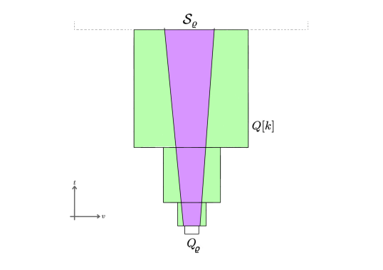
Figure 4. The stacked propagation geometry in the proof of the weak Harnack inequality in Theorem 1.2, as introduced in [32, Section 10].

Step 3: the weak Harnack estimate (1.6)

We prove that for any $k\geq 1$ it holds

(5.5) $$\left|\left\{f>\bar{M}^{k}\right\}\cap{Q}_{r}^{-}\right|\,\leq\,c_{w.h.i.}\bar{\delta}^{k}\,,$$

for some universal constant ${\bar{M}}$, $c$ and $\bar{\delta}\in(0,1)$.

We start by induction. For $k=1$, we simply choose $c$ and $\bar{\delta}$ so that

$$|{Q}_{r}^{-}|\leq c\bar{\delta}.$$

Assume now that (5.5) holds true up to rank $k$ and prove it for $k+1$. Let us consider the following sets,

$$E:=\{f\geq\bar{M}^{k+1}\}\cap{Q}_{r}^{-}\quad\text{and}\quad F:=\{f>\bar{M}^{k}\}\cap{Q}_{1}.$$

Clearly, by recalling the definition (1.7), we infer the sets $E\subset F\subset{Q}_{1}$ are bounded and measurable. Let us consider a cylinder ${Q}_{\sigma}(t_{0},x_{0},v_{0})\subset{Q}_{r}^{-}$, for some $\sigma\in(0,\sigma_{0})$, such that

$$|{Q}_{\sigma}(t_{0},x_{0},v_{0})\cap E|>\bar{\delta}|{Q}_{\sigma}(t_{0},x_{0},v_{0})|.$$

Hence,

(5.6) $$\left|\left\{f\geq\bar{M}^{k+1}\right\}\cap{Q}_{\sigma}(t_{0},x_{0},v_{0})\right|>\bar{\delta}|{Q}_{\sigma}(t_{0},x_{0},v_{0})|.$$

We apply now the procedure enlightened in Step 2 to the function $f$, starting from ${Q}_{\sigma}(t_{0},x_{0},v_{0})$. Hence, recalling (5.6) for any $(t,x,v)\in(t_{0},x_{0},v_{0})\circ\mathcal{S}_{\sigma}$, and recalling that it also contains ${Q}_{r}^{+}$, it holds true the following statement,

$$1\,\geq\,\bar{M}^{k}\left(1+\frac{t-t_{0}}{\sigma^{2s}}\right)^{-q}\,\Longrightarrow\ \sigma\,<\,\bar{M}^{-\frac{k}{2sq}}(t-t_{0})^{\frac{1}{2s}}\,<\,\bar{M}^{-\frac{k}{2sq}}.$$

Now, note that by definition of stacked cylinder $\bar{{Q}}_{\sigma}^{m}(t_{0},x_{0},v_{0})$ in (2.1) we get that $t-t_{0}\leq m\sigma^{2s}$. Hence, we have that $\bar{{Q}}_{\sigma}^{m}(t_{0},x_{0},v_{0})\subset{Q}_{1}$ whenever $\sigma<m^{-2s}$, but this follows by the above estimate up to choosing $\bar{M}$ sufficiently large. Applying now the argument of Step 1 to the function $f((t_{0},x_{0},v_{0})\circ\cdot)$, with $\varrho=\sigma$, $k=m-1$ and choosing $M:=\vartheta^{-m}\bar{M}^{k}$ we get that $\bar{{Q}}_{\sigma}^{m}(t_{0},x_{0},v_{0})\subset F$.

Thus, by the Ink-spot Theorem 2.1 (with $\mu:=1-\bar{\delta}$ and $r_{0}:=\bar{M}^{-\frac{k}{2sq}}$ ) we get

$$\begin{split}&|\{f\geq\bar{M}^{k+1}\}\cap{Q}_{r}^{-}|\\[3.44444pt] &\quad\leq\frac{1+m}{m}(1-c(1-\bar{\delta}))\big{(}|\{f>\bar{M}^{k}\}\cap{Q}_{r}^{-}|+Cmr_{0}^{2s}\big{)}\\[3.44444pt] &\quad\leq\frac{1+m}{m}(1-c(1-\bar{\delta}))\big{(}c_{w.h.i.}\bar{\delta}^{k}+cm\bar{M}^{-\frac{k}{q}}\big{)}\quad\text{\big{(}by the induction step~{}\eqref{eq:ind-weak}\big{)}}\\[3.44444pt] &\quad\leq\frac{1+m}{m}(1-c(1-\bar{\delta}))\big{(}1+c_{w.h.i.}^{-1}cm\big{)}c_{w.h.i.}\bar{\delta}^{k}\quad\text{\big{(}choosing~{}$\bar{\delta}>\bar{M}^{-1/q}\big{)}$}\\[3.44444pt] &\quad\leq c_{w.h.i.}\bar{\delta}^{k+1}\,,\end{split}$$

up to choosing $m$ and consequently $c_{w.h.i.}$ large enough. This proves the desired induction step. The proof of estimate (1.6) will then follow by a standard argument via the layer-cake formula.

6. A new Besicovitch-type covering for slanted cylinders

In particular, as mentioned in the Introduction, we will rely on a new covering argument for the involved slanted cylinders. Such a general Besicovitch-type result will be presented right below.

The following properties for the slanted cylinders in (2.3) do hold true:

1. (Monotonicity) Given a slanted cylinder $Q_{\sigma}(t,x,v)$, and $\varrho>0$, there exist a point $(t^{\prime},x^{\prime},v^{\prime})$ and two constant $\varkappa,\varepsilon>0$ such that

   $$\begin{split}&\|(t,x,v)^{-1}\circ(t^{\prime},x^{\prime},v^{\prime})\|_{\rm kin}\,\leq\,\varepsilon\big{(}\frac{\varkappa\sigma}{\varrho}\big{)}\,,\\ \text{and}\quad&Q_{\frac{\varkappa\sigma}{\varrho}}(t^{\prime},x^{\prime},v^{\prime})\subset Q_{\sigma}(t,x,v)\subset Q_{\frac{\sigma}{\varkappa\varrho}}(t^{\prime},x^{\prime},v^{\prime})\,.\end{split}$$

2. (Exclusion) There exists $\gamma>0$ such that for any $Q_{\varrho}(t_{0},x_{0},v_{0})$ and $(t,x,v)\not\in Q_{\varrho}(t_{0},x_{0},v_{0})$ it holds

   $$\begin{split}Q_{\epsilon^{\gamma}}(t,x,v)\cap Q_{(1-\epsilon)\varrho}(t_{0},x_{0},v_{0})=\emptyset\quad\text{for any}~{}0<\epsilon<1.\end{split}$$

3. (Inclusion) There exists $\wp>1$ such that for $0<\sigma<\varrho<1$ and $(t,x,v)\in Q_{\varrho}(t_{0},x_{0},v_{0})$ it holds

   $$Q_{(\varrho-\sigma)^{\wp}}(t,x,v)\subset Q_{\varrho}(t_{0},x_{0},v_{0}).$$

4. (Engulfment) There exists a constant $\kappa\equiv\kappa(s)$ such that for any ${Q}_{\varrho}(t_{0},x_{0},v_{0})$ and $Q_{\sigma}(t,x,v)$ with

   $$Q_{\varrho}(t_{0},x_{0},v_{0})\cap Q_{\sigma}(t,x,v)\neq\emptyset\quad\text{and}\quad 2\varrho\geq\sigma\,,$$

   it holds that

   $$Q_{\sigma}(t,x,v)\subset\kappa Q_{\varrho}(t_{0},x_{0},v_{0})\,,$$

   with

   $$\begin{split}\kappa Q_{\varrho}(t_{0},x_{0},v_{0})&:=\Big{\{}(t,x,v)\ :\ -\frac{\kappa^{2s}+1}{2}\varrho^{2s}<t-t_{0}\leq\frac{\kappa^{2s}-1}{2}\varrho^{2s}\\ &\qquad\quad|v-v_{0}|<\kappa\varrho,\ \left|x-x_{0}-(t-t_{0})v_{0}\right|<(\kappa\varrho)^{1+2s}\Big{\}}.\end{split}$$

The quantity $\|\cdot\|_{\rm kin}$ is that obtained via the customary kinetic distance, firstly seen in [33] for proving Schauder estimates for Boltzmann equations; that is,

$$\|(t,x,v)\|_{\rm kin}:=\max\big{\{}|t|^{\frac{1}{2s}},\,|x|^{\frac{1}{1+2s}},\,|v|\big{\}}.$$

Compare, also, our Engulfment with Lemma 10.4 there.

We can now state and prove the following

Lemma 6.1 (Besicovitch’s covering Lemma for slanted cylinders).

Let $\varOmega\subset\mathds{R}^{2n+1}$ be a bounded set. Assume that for any $(t,x,v)\in\varOmega$ there exists a family of slanted cylinders $Q_{r}(t,x,v)$ with $r\leq R$, for some $R>0$. Then, there exists a countable family $\Im:=\left\{Q_{r_{k}}(t_{k},x_{k},v_{k})\right\}_{k\in\mathds{N}}$ with the following properties

1. $\displaystyle\varOmega\subset\bigcup_{k=1}^{\infty}Q_{r_{k}}(t_{k},x_{k},v_{k})$.

2. $\displaystyle(t_{k},x_{k},v_{k})\not\in\bigcup_{j<k}Q_{r_{k}}(t_{j},x_{j},v_{j})$, for any $k\geq 2$.

3. For $\epsilon>0$ depending only on the Monotonicity constants $\varkappa$ and $\varepsilon$, the family $\Im_{\epsilon}:=\left\{Q_{(1-\epsilon)r_{k}}(t_{k},x_{k},v_{k})\right\}_{k\in\mathds{N}}$ has bounded overlaps. Moreover,

   $$\sum_{k=1}^{\infty}\chi_{Q_{(1-\epsilon)r_{k}}(t_{k},x_{k},v_{k})}(t,x,v)\,\leq\,c\log\big{(}\frac{1}{\epsilon}\big{)}\,,$$

   where the constant $c$ depends only on $\varkappa$, $\varepsilon$, and the Exclusion constant $\gamma$.

Proof.

Let us assume with no loss of generality that $R:=\sup\left\{r:Q_{r}(t,x,v)\in\Im\right\}$. We set

$$\Im_{0}:=\left\{Q_{r}(t,x,v):\frac{R}{2}<r\leq R,\ Q_{r}(t,x,v)\in\Im\right\}\,,$$

and

$$O_{0}:=\big{\{}(t,x,v):Q_{r}(t,x,v)\in\Im_{0}\big{\}}.$$

Let us choose $Q_{r_{1}}(t_{1},x_{1},v_{1})\in\Im_{0}$. If $O_{0}\subset Q_{r_{1}}(t_{1},x_{1},v_{1})$, then we stop. Otherwise, let us choose $Q_{r_{2}}(t_{2},x_{2},v_{2})$ so that

• $Q_{r_{2}}(t_{2},x_{2},v_{2})\in\Im_{0}$;

• $(t_{2},x_{2},v_{2})\in O_{0}\setminus Q_{r_{1}}(t_{1},x_{1},v_{1})$.

Now, if $O_{0}\subset Q_{r_{1}}(t_{1},x_{1},v_{1})\cup Q_{r_{2}}(t_{2},x_{2},v_{2})$, then we stop, otherwise we continue to iterate such a process. In such a way, we build a subfamily $\Im_{0}^{\prime}:=\left\{Q_{r_{j}^{0}}(t_{j}^{0},x_{j}^{0},v_{j}^{0})\right\}_{j\in\mathds{N}}$ such that $\displaystyle(t_{k}^{0},x_{k}^{0},v_{k}^{0})\in O_{0}\setminus\bigcup_{j<k}Q_{r_{j}^{0}}(t_{j}^{0},x_{j}^{0},v_{j}^{0})$.

Now, we consider the following families,

$$\Im_{1}:=\left\{Q_{r}(t,x,v):\frac{R}{4}<r\leq\frac{R}{2},\ Q_{r}(t,x,v)\in\Im\right\}\,,$$

and

$$O_{1}:=\left\{(t,x,v)\,:\,Q_{r}(t,x,v)\in\Im_{1}\ \text{and}\,~{}(t,x,v)\not\in\bigcup_{j=1}^{\infty}Q_{r_{j}^{0}}(t_{j}^{0},x_{j}^{0},v_{j}^{0})\right\}.$$

In a similar fashion as above we build a family $\Im_{1}^{\prime}:=\left\{Q_{r_{j}^{1}}(t_{j}^{1},x_{j}^{1},v_{j}^{1})\right\}_{j\in\mathds{N}}$ such that $\displaystyle(t_{k}^{1},x_{k}^{1},v_{k}^{1})\in O_{1}\setminus\bigcup_{j<k}Q_{r_{j}^{1}}(t_{j}^{1},x_{j}^{1},v_{j}^{1})$.

By iterating this process up to the $k^{\rm th}$-stage, we obtain the following two families,

$$\Im_{k}:=\left\{Q_{r}(t,x,v):\frac{R}{2^{k+1}}<r\leq\frac{R}{2^{k}},\ Q_{r}(t,x,v)\in\Im\right\}\,,$$

and

$$O_{k}:=\left\{(t,x,v):Q_{r}(t,x,v)\in\Im_{k}\ \text{and}\,~{}(t,x,v)\not\in\bigcup_{i=0}^{k-1}\bigcup_{j=1}^{\infty}Q_{r_{j}^{i}}(t_{j}^{i},x_{j}^{i},v_{j}^{i})\right\}.$$

From this, we get a family of cylinders $\Im_{k}^{\prime}:=\left\{Q_{r_{j}^{k}}(t_{j}^{k},x_{j}^{k},v_{j}^{k})\right\}_{j\in\mathds{N}}$  so that $\displaystyle(t_{\ell}^{k},x_{\ell}^{k},v_{\ell}^{k})\in O_{k}\setminus\bigcup_{j<\ell}Q_{r_{j}^{k}}(t_{j}^{k},x_{j}^{k},v_{j}^{k})$.

We now are in the position to prove that the collection of all slanted cylinders in all $\Im_{k}^{\prime}$ do satisfy the conditions of Lemma 6.1.

We start by proving that each family $\Im^{\prime}_{i}$ has bounded overlapping. For this, suppose that

$$(t,x,v)\in Q_{r_{j_{1}}^{i}}(t_{j_{1}}^{i},x_{j_{1}}^{i},v_{j_{1}}^{i})\,\cap\,...\,\cap\,Q_{r_{j_{m}}^{i}}(t_{j_{m}}^{i},x_{j_{m}}^{i},v_{j_{m}}^{i})\,,$$

with $Q_{r_{j_{\ell}}^{i}}(t_{j_{\ell}}^{i},x_{j_{\ell}}^{i},v_{j_{\ell}}^{i})\in\Im^{\prime}_{i}$. Now, let $Q_{r_{0}^{i}}(t_{0}^{i},x_{0}^{i},v_{0}^{i})$ be the cylinder with $r_{0}^{i}:=\max\left\{r_{j_{\ell}}^{i}:1\leq\ell\leq m\right\}$. Note that, by construction, we can also assume that $(t_{j_{N}}^{i},x_{j_{N}}^{i},v_{j_{N}}^{i})\not\in Q_{r_{j_{\ell}}^{i}}(t_{j_{\ell}}^{i},x_{j_{\ell}}^{i},v_{j_{\ell}}^{i})$, for $\ell<N$.

In view of the Monotonicity property of the slanted cylinder, we have that there exist $\varkappa$, $\varepsilon>0$ such that

(6.1) $$\begin{split}&\|(t_{j_{\ell}}^{i},x_{j_{\ell}}^{i},v_{j_{\ell}}^{i})^{-1}\circ(t_{\ell}^{\prime},x_{\ell}^{\prime},v_{\ell}^{\prime})\|_{\rm kin}\,\leq\,\varepsilon\big{(}\frac{\varkappa r_{j_{\ell}}^{i}}{r_{0}^{i}}\big{)}\,,\\[4.30554pt] \text{and}\quad&Q_{\frac{\varkappa r_{j_{\ell}}^{i}}{r_{0}^{i}}}(t_{\ell}^{\prime},x_{\ell}^{\prime},v_{\ell}^{\prime})\,\subset\,Q_{r_{j_{\ell}}^{i}}(t_{j_{\ell}}^{i},x_{j_{\ell}}^{i},v_{j_{\ell}}^{i})\,\subset\,Q_{\frac{r_{j_{\ell}}^{i}}{\varkappa r_{0}^{i}}}(t_{\ell}^{\prime},x_{\ell}^{\prime},v_{\ell}^{\prime})\,,\end{split}$$

for any $1\leq\ell\leq m$. Recalling that $(t_{j_{N}}^{i},x_{j_{N}}^{i},v_{j_{N}}^{i})\not\in Q_{r_{j_{\ell}}^{i}}(t_{j_{\ell}}^{i},x_{j_{\ell}}^{i},v_{j_{\ell}}^{i})$, we get by (6.1) that, for $N>\ell$,

(6.2) $$(t_{j_{N}}^{i},x_{j_{N}}^{i},v_{j_{N}}^{i})\not\in Q_{\frac{\varkappa r_{j_{\ell}}^{i}}{r_{0}^{i}}}(t_{\ell}^{\prime},x_{\ell}^{\prime},v_{\ell}^{\prime}).$$

Then, by combining (6.1) with (6.2) we have that

$$\|(t_{j_{N}}^{i},x_{j_{N}}^{i},v_{j_{N}}^{i})^{-1}\circ(t_{j_{\ell}}^{i},x_{j_{\ell}}^{i},v_{j_{\ell}}^{i})\|_{\rm kin}$$

$$\qquad\geq\,\|(t_{j_{N}}^{i},x_{j_{N}}^{i},v_{j_{N}}^{i})^{-1}\circ(t_{\ell}^{\prime},x_{\ell}^{\prime},v_{\ell}^{\prime})\|_{\rm kin}-\|(t_{j_{\ell}}^{i},x_{j_{\ell}}^{i},v_{j_{\ell}}^{i})^{-1}\circ(t_{\ell}^{\prime},x_{\ell}^{\prime},v_{\ell}^{\prime})\|_{\rm kin}$$

(6.3) $$\qquad>\,\frac{\varkappa r_{j_{\ell}}^{i}}{r_{0}^{i}}\big{(}1-\varepsilon\big{)}\,>\,c(\varkappa,\varepsilon)\,>\,0\,,$$

since $R2^{-(i+1)}<r_{j_{\ell}}^{i}\leq r_{0}^{i}\leq R2^{-i}$. Moreover, by taking into account (6.2), we have that $Q_{r_{j_{\ell}}^{i}}(t_{j_{\ell}}^{i},x_{j_{\ell}}^{i},v_{j_{\ell}}^{i})$ is contained in a slanted cylinder $Q_{\mathfrak{R}}({\bf 0})$, with the radius $\mathfrak{R}$ depending only on $\varkappa$ and $\varepsilon$. By (6), proceeding as in [10, Lemma 1], we obtain that the overlapping in each family $\Im_{i}^{\prime}$ is at most $\alpha$, with $\alpha$ depending only on $\kappa,\varepsilon$ and the dimension $n$ only.

Now, we prove that the family $\Im_{i}^{\prime}$ is finite. Since $\varOmega$ is bounded and $R2^{-(i+1)}<r_{j}^{i}\leq R2^{-i}$, there exists a constant $C>0$ such that $O_{i}\subset Q_{Cr^{i}_{1}}(t^{i}_{1},x^{i}_{1},v^{i}_{1})$ and $Cr_{1}^{i}\geq R2^{-i}$. Then, for any $Q_{r^{i}_{j}}(t^{i}_{j},x^{i}_{j},v^{i}_{j})\in\Im_{i}^{\prime}$ we get

(6.4) $$Q_{\frac{\varkappa}{2C}}(t^{\prime}_{j},x^{\prime}_{j},v^{\prime}_{j}) \subset Q_{r^{i}_{j}}(t^{i}_{j},x^{i}_{j},v^{i}_{j})$$

$$\subset Q_{\frac{r^{i}_{j}}{C\varkappa r_{1}^{i}}}(t^{\prime}_{j},x^{\prime}_{j},v^{\prime}_{j})$$

$$\subset Q_{\frac{1}{C\varkappa}}(t^{\prime}_{j},x^{\prime}_{j},v^{\prime}_{j})\ \subset\ Q_{\Re}({\bf 0})\,,$$

with $\Re$ depending only on $C$ and $\varkappa$.

Since $\Im_{i}^{\prime}$ has overlapping bounded by $\alpha$, we get

$$\sum_{j=1}^{\infty}\chi_{Q_{r^{i}_{j}}(t^{i}_{j},x^{i}_{j},v^{i}_{j})}(t,x,v)\leq\alpha\,,$$

which, in view of (6.4), implies

$$\sum_{j=1}^{\infty}\chi_{Q_{\frac{\varkappa}{2C}}(t^{\prime}_{j},x^{\prime}_{j},v^{\prime}_{j})}(t,x,v)\,\leq\,\alpha\chi_{Q_{\Re}({\bf 0})}\,.$$

Hence, iterating the sums above we deduce that $\Im_{i}^{\prime}$ has a finite number of cylinders.

We now estimate the boundedness of overlapping between different generators of the families $\Im_{i}^{\prime}$. We start by shrinking the selected cylinders

(6.5) $$(t_{0},x_{0},v_{0})\in\bigcap_{i=1}^{\infty}Q_{(1-\epsilon)r_{j_{i}}^{e_{i}}}(t_{j_{i}}^{e_{i}},x_{j_{i}}^{e_{i}},v_{j_{i}}^{e_{i}})\,,$$

with $e_{1}<e_{2}<\dots$, $R2^{-(e_{i}+1)}<r_{j_{i}}^{e_{i}}\leq R2^{-e_{i}}$. Fix now, $i$ and $\ell>i$, let us measure the gap between $e_{i}$ and $e_{\ell}$. Since $r_{j_{\ell}}^{e_{\ell}}<r_{j_{i}}^{e_{i}}$ we have that

$$Q_{\frac{\varkappa(1-\epsilon)r_{j_{\ell}}^{e_{\ell}}}{r_{j_{i}}^{e_{i}}}}(t^{\prime},x^{\prime},v^{\prime})\,\subset\,Q_{r_{j_{\ell}}^{e_{\ell}}}(t_{j_{\ell}}^{e_{\ell}},x_{j_{\ell}}^{e_{\ell}},v_{j_{\ell}}^{e_{\ell}})\,\subset\,Q_{\frac{(1-\epsilon)r_{j_{\ell}}^{e_{\ell}}}{\varkappa r_{j_{i}}^{e_{i}}}}(t^{\prime},x^{\prime},v^{\prime}).$$

Moreover, by the Exclusion property we have that

$$Q_{\epsilon^{\gamma}}(t_{j_{\ell}}^{e_{\ell}},x_{j_{\ell}}^{e_{\ell}},v_{j_{\ell}}^{e_{\ell}})\cap Q_{(1-\epsilon)r_{j_{i}}^{e_{i}}}(t_{j_{i}}^{e_{i}},x_{j_{i}}^{e_{i}},v_{j_{i}}^{e_{i}})=\emptyset.$$

Thus,

$$0 < \epsilon^{\gamma}$$

$$< \|(t_{j_{\ell}}^{e_{\ell}},x_{j_{\ell}}^{e_{\ell}},v_{j_{\ell}}^{e_{\ell}})^{-1}\circ(t_{0},x_{0},v_{0})\|_{\rm kin}$$

$$\leq \|(t^{\prime},x^{\prime},v^{\prime})^{-1}\circ(t_{0},x_{0},v_{0})\|_{\rm kin}+\|(t_{j_{\ell}}^{e_{\ell}},x_{j_{\ell}}^{e_{\ell}},v_{j_{\ell}}^{e_{\ell}})^{-1}\circ(t^{\prime},x^{\prime},v^{\prime})\|_{\rm kin}$$

$$\leq \frac{(1-\epsilon)r_{j_{\ell}}^{e_{\ell}}}{\varkappa r_{j_{i}}^{e_{i}}}+\varepsilon\frac{\varkappa(1-\epsilon)r_{j_{\ell}}^{e_{\ell}}}{r_{j_{i}}^{e_{i}}}\ \lesssim\ 2^{e_{i}-e_{\ell}}\,,$$

which yields

$$e_{\ell}-e_{i}\lesssim\log_{2}\big{(}\frac{1}{\epsilon}\big{)}\,,$$

up to a constant, depending only on $\varepsilon$, $\varkappa$, and the Exclusion constant $\gamma$.

All in all, the number of cylinders in (6.5) is bounded by a multiple of $\log_{2}\big{(}\frac{1}{\epsilon}\big{)}$, up to a multiplicative constant which – we recall – will depend only on $\varepsilon$, $\varkappa$ and $\gamma$.

Now consider the family $\Im^{\prime}:=\{\Im_{i}^{\prime}\}_{i=1}^{\infty}$. Since any family $\Im_{i}^{\prime}$ covers $O_{i}$, the family $\Im^{\prime}$ cover $\varOmega$, so (i) follows. Moreover, up to relabelling the cylinders, one can deduce (ii). Finally, by the argument above, also (iii) is satisfied up to enlarging the constant. ∎

7. Proof of the strong Harnack inequality

This section is devoted to the completion of the proof of the strong Harnack inequality in Theorem 1.3. Armed with the weak Harnack estimate in (1.6) obtained in the preceding section, as well as with the feasibility of the $L^{\infty}$-estimates in Section 3 via their $\delta$-interpolative parameter, in order to concretize our final strategy we will just need a nonlocal tail control before going into the Besicovitch-type covering argument presented in Section 6; see Lemma 7.1 below. As already said, the whole strategy below seems feasible to attack several different kinetic integral problems when the related ingredients will be cooked as in the preceding sections.

Lemma 7.1 (Kinetic Tail control).

For any $s\in(0,1)$, let $f\in\mathcal{W}$ be a nonnegative weak solution to (1.1) in $\varOmega$ and let ${Q}_{1}({\bf 0})\equiv{Q}_{1}\subset\varOmega$. Then, for any $p>1$ and any ${Q}_{2R}({\bf 0})\equiv{Q}_{2R}\subset{Q}_{1}$, it holds

(7.1) $${\rm Tail}_{p}(f;{\bf 0},R,r)\,\leq\,c\sup_{Q_{2R}}f\qquad\forall r\in(0,{2R}]\,,$$

where the positive constant $c$ depends only on $n,s$ and $\varLambda$; the nonlocal kinetic tail ${\rm Tail}_{p}$ being the quantity defined in (2.1).

Proof.

Consider the classical shifted approximating sequence $\{f_{k}\}_{k\in\mathds{N}}$ defined by $f_{k}=f_{k}(t,x,v):=f(t,x,v)+1/k$, for any $k\geq 1$, and take a cut-off function in velocity $\phi=\phi(v)$ such that $\phi(v)\equiv 0$ in $\mathds{R}^{n}\setminus B_{r/2}$ and ${|\nabla_{v}\phi|\leq c/r}$. Notice that for any $k\geq 1$, the strictly positive sequence $f_{k}$ is such that the Gagliardo numerator in the integral diffusion satisfy the immediate equality

(7.2) $$\big{(}f_{k}(\cdot,\cdot,v)-f_{k}(\cdot,\cdot,w)\big{)}=\big{(}f(\cdot,\cdot,v)-f(\cdot,\cdot,w)\big{)}$$

Now, we will estimate the nonlocal energy $\mathcal{E}$ in virtue of the the following function $\phi_{k}$ given by

(7.3) $$\phi_{k}(t,x,v):=\frac{\phi^{2}(v)}{\sqrt{f_{k}(t,x,v)}},\quad\text{for any fixed}\ k\geq 1.$$

This is quite standard, and, as one would expect, the desired tail quantity will come from the integral diffusion energy by splitting the double integral contributions thanks to the smoothness of the chosen cut-off function $\phi$, as for instance elsewhere in the elliptic counterpart in [15, 16] as well as elsewhere in the present manuscript (see, e .g., the estimates in the proof of Theorem 1.1). For the sake of simplicity, let assume that the symmetric kernel $K$ does coincide with the Gagliardo one; this is not restrictive here because of (2.4), so that the constant in (7.1) will also depend by $\varLambda$. We have

$$\mathcal{E}(f(t,x,\cdot),\phi_{k}(t,x,\cdot))$$

$$\qquad=\ \int_{B_{r}}\int_{B_{r}}\frac{\big{(}f(t,x,v)-f(t,x,w)\big{)}}{|v-w|^{n+2s}}\big{(}\phi_{k}(t,x,v)-\phi_{k}(t,x,w)\big{)}\,\,{\rm d}v\,{\rm d}w$$

$$\qquad+\ 2\int_{\mathds{R}^{n}\setminus B_{r}}\int_{B_{r}}\frac{\big{(}f(t,x,v)-f(t,x,w)\big{)}}{|v-w|^{n+2s}}\big{(}\phi_{k}(t,x,v)-\phi_{k}(t,x,w)\big{)}\,\,{\rm d}v\,{\rm d}w$$

(7.4) $$\qquad=:I_{1}+I_{2}$$

We estimate $I_{1}$ in the display above making use of the observation in (7.2) and the symmetry of the kernel. Indeed, simply observing that

$$\big{(}f(v)-f(w)\big{)}\big{(}\phi_{k}(v)-\phi_{k}(w)\big{)}$$

$$\qquad=\sqrt{f_{k}(v)}\phi^{2}(v)+\sqrt{f_{k}(w)}\phi^{2}(w)-f_{k}(w)\frac{\phi^{2}(v)}{\sqrt{f_{k}(v)}}-f_{k}(v)\frac{\phi^{2}(w)}{\sqrt{f_{k}(w)}}$$

$$\qquad=\big{(}\sqrt[4]{f_{k}(v)}\phi(v)-\sqrt[4]{f_{k}(w)}\phi(w)\big{)}^{2}$$

$$\qquad\quad-\Big{(}f_{k}(w)\frac{\phi^{2}(v)}{\sqrt{f_{k}(v)}}+f_{k}(v)\frac{\phi^{2}(w)}{\sqrt{f_{k}(w)}}-2\sqrt[4]{f_{k}(v)}\sqrt[4]{f_{k}(w)}\phi(v)\phi(w)\Big{)}$$

$$\qquad=\big{(}\sqrt[4]{f_{k}(v)}\phi(v)-\sqrt[4]{f_{k}(w)}\phi(w)\big{)}^{2}-\Big{(}\sqrt{f_{k}(w)}\frac{\phi(v)}{\sqrt[4]{f_{k}(v)}}-\sqrt{f_{k}(v)}\frac{\phi(w)}{\sqrt[4]{f_{k}(w)}}\Big{)}^{2}$$

(7.5) $$\qquad\leq\,\big{(}\sqrt[4]{f_{k}(v)}\phi(v)-\sqrt[4]{f_{k}(w)}\phi(w)\big{)}^{2}\,.$$

So that, the symmetric part in (7), can be treated as follows (assuming $f_{k}(w)\geq f_{k}(v)$ up to exchange the role of $v$ and $w$) applying (7)

(7.6) $$I_{1} \leq \int_{B_{r}}\sqrt{f_{k}(w)}\int_{B_{r}}\frac{|\phi(v)-\phi(w)|^{2}\,{\rm d}v}{\lvert v-w\rvert^{n+2s}}\,{\rm d}w$$

$$\leq \frac{c}{r^{2}}\int_{B_{r}}\sqrt{f_{k}(w)}\int_{B_{2r}(w)}\frac{\,{\rm d}v}{\lvert v-w\rvert^{n-2(1-s)}}\,{\rm d}w$$

$$\leq \frac{cr^{-2s}}{2(1-s)}\|\sqrt{f_{k}}\|_{L^{1}(B_{r})}\,,$$

where we also used both the aforementioned cancelation property and the smoothness of the cut-off function $\phi$.

As mentioned, the desired (elliptic) nonlocal tail contribution is basically in the last integral $I_{2}$ in (7). We have

$${I_{2}/2}\ =\ \int_{\mathds{R}^{n}\setminus B_{r}}\int_{B_{r}}\frac{\big{(}f(t,x,v)-f(t,x,w)\big{)}}{|v-w|^{n+2s}}\big{(}\phi_{k}(t,x,v)-\phi_{k}(t,x,w)\big{)}\,\,{\rm d}v\,{\rm d}w\,.$$

$$\qquad\qquad=\int_{\mathds{R}^{n}\setminus B_{r}}\int_{\text{supp}~{}\phi}\frac{\frac{f(t,x,v)}{\sqrt{f_{k}(v)}}}{|v-w|^{n+2s}}\phi^{2}(v)\,\,{\rm d}v\,{\rm d}w$$

$$\qquad\qquad\quad\ -\,\int_{\mathds{R}^{n}\setminus B_{r}}\int_{\text{supp}~{}\phi}\frac{\frac{f(t,x,w)}{\sqrt{f_{k}(v)}}}{|v-w|^{n+2s}}\phi^{2}(v)\,\,{\rm d}v\,{\rm d}w$$

(7.7) $$\qquad\qquad\leq\ c{r^{-2s}}\|\sqrt{f_{k}}\|_{L^{1}(B_{r})}-c\left(\int_{B_{r}}\frac{1}{\sqrt{f_{k}(v)}}\,{\rm d}v\right)\left(\int_{\mathds{R}^{n}\setminus B_{r}}\frac{f(w)}{|w|^{n+2s}}\,\,{\rm d}w\right),$$

where in the last inequality we have also used that $\text{supp}~{}\phi\subset B_{r}$, as for instance already seen in the middle of proof of Theorem 1.1.

Thus, by combining (7) with (7.6) and (7), up to relabeling the constant $c$, we get the following estimate in the nonlocal energy $\mathcal{E}(f,\phi_{k})$,

$$\mathcal{E}(f(t,x,\cdot),\phi_{k}(t,x,\cdot))$$

(7.8) $$\qquad\quad\qquad\leq\ c\,{r^{-2s}}\|\sqrt{f_{k}}\|_{L^{1}(B_{r})}$$

$$\qquad\qquad\quad\quad\ -\,c\left(\int_{B_{r}}\frac{1}{\sqrt{f_{k}(v)}}\,{\rm d}v\right)\left(\int_{\mathds{R}^{n}\setminus B_{r}}\frac{f(w)}{|w|^{n+2s}}\,\,{\rm d}w\right),$$

which does hold in $U_{r}$ for any $n\geq 1$.

Now, it remains to treat the transport term, which can be treated as in the classical Kolmogorov-Fokker-Planck equation, since – in view of the inequality above – we already isolated the desired tail quantity which is basically, so that we can finally extract the supremum of the sequence approximating the solution $f$. Indeed, we will make use of the classical cut-off function depending only on the trasport variables, combined with a standard integration by parts for the transport term in the equation; compare for instance with the energies estimates in [22].

We will also make use of the fact that $f$ is a subsolution to (1.1), by choosing an appropriate test function in Definition 2.2. For this, we consider a cut-off $\psi\equiv\psi(x,t)$ such that $\psi\equiv 1$ on $U_{R}$ and $\psi\equiv 0$ outside $U_{2R}$ with

$$\psi(0,\cdot)=0\quad\text{and}\quad\left|[\partial_{t}+v\cdot\nabla_{x}]\psi\right|\sim{R^{-2s}}\,,$$

which will combined with the sequence $\phi_{k}$ above. We then deduce that

(7.9) $$-\int_{\mathds{R}^{n}}\big{[}(\partial_{t}+v\cdot\nabla_{x})f\big{]}\phi_{k}\psi^{2}\,{\rm d}v-\mathcal{E}(f,\phi_{k})\psi^{2}=0\quad\text{for a.~{}\!e.}\ (t,x)\in U_{2R}\,,$$

where we also used a standard Besicovitch-Lebesgue differentiation in view of the fact that $\textrm{supp}\,\psi\subset U_{2R}$.

Now, taking the supremum over time and space of the transport term, noting that $\sup(-a(x,t))=-\inf a(x,t)$, we then apply the mean value theorem over $U_{2R}$ obtaining from (7.9) that

$$-\mathchoice{\mathop{\kern 1.99997pt\vrule width=6.00006pt,height=3.0pt,depth=-2.49997pt\kern-8.00003pt\intop}\nolimits_{\kern-2.79996ptU_{2R}}}{\mathop{\kern 1.00006pt\vrule width=5.0pt,height=3.0pt,depth=-2.59996pt\kern-6.00006pt\intop}\nolimits_{U_{2R}}}{\mathop{\kern 1.00006pt\vrule width=5.0pt,height=3.0pt,depth=-2.59996pt\kern-6.00006pt\intop}\nolimits_{U_{2R}}}{\mathop{\kern 1.00006pt\vrule width=5.0pt,height=3.0pt,depth=-2.59996pt\kern-6.00006pt\intop}\nolimits_{U_{2R}}}\int_{\mathds{R}^{n}}\big{[}(\partial_{t}+v\cdot\nabla_{x})f\big{]}\phi_{k}\psi^{2}\,{\rm d}v-\mathcal{E}(f,\phi_{k})\psi^{2}\leq 0\,.$$

Integrating by parts the transport term and recalling the particular choice of the test function yields

$$\left(\int_{B_{r}}\frac{1}{\sqrt{f_{k}(v)}}\,{\rm d}v\right)\left(\int_{\mathds{R}^{n}\setminus B_{r}}\frac{f(w)}{|w|^{n+2s}}\,\,{\rm d}w\right)\psi^{2}(x,t)$$

(7.10) $$\qquad\qquad\leq\,c{r^{-2s}}\|\sqrt{f_{k}}\|_{L^{1}(B_{r})}\psi^{2}(x,t)+c{R^{-2s}}\mathchoice{\mathop{\kern 1.99997pt\vrule width=6.00006pt,height=3.0pt,depth=-2.49997pt\kern-8.00003pt\intop}\nolimits_{\kern-2.79996ptU_{2R}}}{\mathop{\kern 1.00006pt\vrule width=5.0pt,height=3.0pt,depth=-2.59996pt\kern-6.00006pt\intop}\nolimits_{U_{2R}}}{\mathop{\kern 1.00006pt\vrule width=5.0pt,height=3.0pt,depth=-2.59996pt\kern-6.00006pt\intop}\nolimits_{U_{2R}}}{\mathop{\kern 1.00006pt\vrule width=5.0pt,height=3.0pt,depth=-2.59996pt\kern-6.00006pt\intop}\nolimits_{U_{2R}}}\int_{B_{r}}\sqrt{f_{k}}\,{\rm d}v\,{\rm d}x\,{\rm d}t\,,$$

where we also applied the estimate in (7).

Moreover, note that the left-hand side of (7) can be estimated as follows,

$$\begin{split}&\left(\int_{B_{r}}\frac{1}{\sqrt{f_{k}(v)}}\,{\rm d}v\right)\left(\int_{\mathds{R}^{n}\setminus B_{r}}\frac{f(w)}{|w|^{n+2s}}\,\,{\rm d}w\right)\\[3.01385pt] &\qquad\qquad\qquad\qquad\geq\ cr^{n}\inf_{B_{r}}\frac{1}{\sqrt{f_{k}(v)}}\left(\int_{\mathds{R}^{n}\setminus B_{r}}\frac{f_{k}(w)}{|w|^{n+2s}}\,\,{\rm d}w\right)\\[3.01385pt] &\qquad\qquad\qquad\qquad=\ \frac{cr^{n}}{\sup\limits_{B_{r}}\sqrt{f_{k}}}\left(\int_{\mathds{R}^{n}\setminus B_{r}}\frac{f_{k}(w)}{|w|^{n+2s}}\,\,{\rm d}w\right)\,.\end{split}$$

So that, from (7) we get

(7.11) $$\left(\int_{\mathds{R}^{n}\setminus B_{r}}\frac{f(w)}{|w|^{n+2s}}\,\,{\rm d}w\right)\psi^{2}(x,t) \leq c\,r^{n-2s}\sup_{B_{r}}\sqrt{f_{k}}\|\sqrt{f_{k}}\|_{L^{1}(B_{r})}\psi^{2}(x,t)$$

$$+c{R^{-2s}}r^{n}\sup_{B_{r}}\sqrt{f_{k}}\mathchoice{\mathop{\kern 1.99997pt\vrule width=6.00006pt,height=3.0pt,depth=-2.49997pt\kern-8.00003pt\intop}\nolimits_{\kern-2.79996ptU_{2R}}}{\mathop{\kern 1.00006pt\vrule width=5.0pt,height=3.0pt,depth=-2.59996pt\kern-6.00006pt\intop}\nolimits_{U_{2R}}}{\mathop{\kern 1.00006pt\vrule width=5.0pt,height=3.0pt,depth=-2.59996pt\kern-6.00006pt\intop}\nolimits_{U_{2R}}}{\mathop{\kern 1.00006pt\vrule width=5.0pt,height=3.0pt,depth=-2.59996pt\kern-6.00006pt\intop}\nolimits_{U_{2R}}}\int_{B_{r}}\sqrt{f_{k}}\,{\rm d}v\,{\rm d}x\,{\rm d}t$$

$$\leq c\,r^{2n-2s}\big{(}\sup_{B_{r}}f_{k}(t,x,\cdot)\big{)}\psi^{2}(t,x)$$

$$+c{R^{-2s}}r^{2n}\big{(}\sup_{B_{r}}\sqrt{f_{k}(t,x,\cdot)}\big{)}\sup_{Q_{2R}}\sqrt{f_{k}}$$

$$\leq cR^{2n{-2s}}\sup_{Q_{2R}}f_{k}\,.$$

Hence, for any $p>1$, by integrating both sides over $U_{R}$ and recalling that $\psi\equiv 1$ on $U_{R}$, it yields

$${\rm Tail}_{p}(f;{\bf 0},R,r)\leq c\,\sup_{Q_{2R}}f_{k}\,,$$

up to relabeling the constant $c$, which gives the desired result, upon passing to the limit for $k\to\infty$. ∎

We are now in the position to finalize the proof of our main result.

Proof of Theorem 1.3.

Firstly, we apply Theorem 1.1. For any $\delta\in(0,1]$ and for any $\varrho$ such that ${Q}_{\varrho}\subset\varOmega$, upon translating the cylinder back in time, it holds

(7.12) $$\sup_{{Q}^{-}_{\frac{\varrho}{2}}}f \leq c\,(\delta{\varrho^{4s}})^{-\frac{1}{2\varepsilon_{*}}}\,\Big{(}\,\int_{{Q}_{\varrho}^{-}}f^{2}\,\,{\rm d}v\,{\rm d}x\,{\rm d}t\Big{)}^{\frac{1}{2}}+\delta\,{\rm Tail}_{p}\big{(}f;(-1+\varrho^{2s},\,0,\,0),\varrho,\frac{\varrho}{2}\big{)}$$

$$\leq c\,(\delta{\varrho^{4s}})^{-\frac{1}{2\varepsilon_{*}}}\,\Big{(}\,\int_{{Q}_{\varrho}^{-}}f^{2}\,\,{\rm d}v\,{\rm d}x\,{\rm d}t\Big{)}^{\frac{1}{2}}+c\delta\sup_{{Q}_{2\varrho}(-1+\varrho^{2s},\,0,\,0)}f\,,$$

where we have also applied the estimate in Lemma 7.1 with $p=p^{\star}$, $R=\varrho$ and $r=\varrho/2$ there, by taking into account the translation in time in the center which does not affect the estimate in (7.1). The positive constant $c$ in (7.12) above does depend only on $n$ and $s$. In this regards, note that we have also tracked the precise dependencies of the constant with respect to the radii in the proof of Theorem 1.1.

Now, let us set $1/2\leq\sigma^{\prime}<\sigma\leq 1$, $\varrho=(\sigma-\sigma^{\prime})^{\wp}$, with $\wp$ being the Inclusion exponent in Section 6, and consider the family of cylinders $\{Q_{(\sigma-\sigma^{\prime})^{\wp}}\}_{1/2\leq\sigma^{\prime}<\sigma\leq 1}$. By taking into account the Inclusion property, any cylinder of this family is contained in $Q_{\sigma}^{-}$. Then, by Lemma 6.1, up to renumbering the family, we can cover $Q_{\sigma^{\prime}}^{-}$ by a family of slanted cylinders with radii less than ${(\sigma-\sigma^{\prime})^{\wp}}/{2}$, up to relabelling $\varrho$ below, and that is by their very construction. Note that we also have that

$${Q}_{(\sigma-\sigma^{\prime})^{\wp}}\left(-1+\left((\sigma-\sigma^{\prime})^{\wp}/2\right)^{2s}\!,\,0,\,0\right)\subset Q_{\sigma}^{-}\,,$$

where the Inclusion property assured that the center $\big{(}-1+\left((\sigma-\sigma^{\prime})^{\wp}/2\right)^{2s}\!,\,0,\,0\big{)}$ belongs to $Q_{\sigma}^{-}$.

Thus, by (7.12), we get

(7.13) $$\sup_{{Q}^{-}_{\sigma^{\prime}}}f \leq \frac{c\,\delta^{-\frac{1}{2\varepsilon_{*}}}}{\big{[}(\sigma-\sigma^{\prime})^{\wp}\big{]}^{\frac{2s}{\varepsilon_{*}}}}\,\Big{(}\,\mathchoice{\mathop{\kern 1.99997pt\vrule width=6.00006pt,height=3.0pt,depth=-2.49997pt\kern-8.00003pt\intop}\nolimits_{\kern-2.79996pt{Q}^{-}_{\sigma}}}{\mathop{\kern 1.00006pt\vrule width=5.0pt,height=3.0pt,depth=-2.59996pt\kern-6.00006pt\intop}\nolimits_{{Q}^{-}_{\sigma}}}{\mathop{\kern 1.00006pt\vrule width=5.0pt,height=3.0pt,depth=-2.59996pt\kern-6.00006pt\intop}\nolimits_{{Q}^{-}_{\sigma}}}{\mathop{\kern 1.00006pt\vrule width=5.0pt,height=3.0pt,depth=-2.59996pt\kern-6.00006pt\intop}\nolimits_{{Q}^{-}_{\sigma}}}f_{+}^{2}\,\,{\rm d}v\,{\rm d}x\,{\rm d}t\Big{)}^{\frac{1}{2}}+\,c\delta\,\,\sup_{{Q}^{-}_{\sigma}}f$$

$$\leq \frac{c\,\delta^{-\frac{1}{2\varepsilon_{*}}}}{\big{[}(\sigma-\sigma^{\prime})^{\wp}\big{]}^{\frac{2s}{\varepsilon_{*}}}}\,\Big{(}\sup_{{Q}^{-}_{\sigma}}f\Big{)}^{\!\frac{2-\zeta}{2}}\Big{(}\,\mathchoice{\mathop{\kern 1.99997pt\vrule width=6.00006pt,height=3.0pt,depth=-2.49997pt\kern-8.00003pt\intop}\nolimits_{\kern-2.79996pt{Q}^{-}_{\sigma}}}{\mathop{\kern 1.00006pt\vrule width=5.0pt,height=3.0pt,depth=-2.59996pt\kern-6.00006pt\intop}\nolimits_{{Q}^{-}_{\sigma}}}{\mathop{\kern 1.00006pt\vrule width=5.0pt,height=3.0pt,depth=-2.59996pt\kern-6.00006pt\intop}\nolimits_{{Q}^{-}_{\sigma}}}{\mathop{\kern 1.00006pt\vrule width=5.0pt,height=3.0pt,depth=-2.59996pt\kern-6.00006pt\intop}\nolimits_{{Q}^{-}_{\sigma}}}f_{+}^{\zeta}\,\,{\rm d}v\,{\rm d}x\,{\rm d}t\Big{)}^{\frac{1}{2}}+\,c\delta\,\,\sup_{{Q}^{-}_{\sigma}}f$$

$$\leq \frac{2-\zeta}{2}\sup_{{Q}^{-}_{\sigma}}f+\frac{c\,\delta^{-\frac{1}{2\varepsilon_{*}}}}{(\sigma-\sigma^{\prime})^{\frac{4s\wp}{\zeta\varepsilon_{*}}}}\Big{(}\,\mathchoice{\mathop{\kern 1.99997pt\vrule width=6.00006pt,height=3.0pt,depth=-2.49997pt\kern-8.00003pt\intop}\nolimits_{\kern-2.79996pt{Q}^{-}_{\sigma}}}{\mathop{\kern 1.00006pt\vrule width=5.0pt,height=3.0pt,depth=-2.59996pt\kern-6.00006pt\intop}\nolimits_{{Q}^{-}_{\sigma}}}{\mathop{\kern 1.00006pt\vrule width=5.0pt,height=3.0pt,depth=-2.59996pt\kern-6.00006pt\intop}\nolimits_{{Q}^{-}_{\sigma}}}{\mathop{\kern 1.00006pt\vrule width=5.0pt,height=3.0pt,depth=-2.59996pt\kern-6.00006pt\intop}\nolimits_{{Q}^{-}_{\sigma}}}f_{+}^{\zeta}\,\,{\rm d}v\,{\rm d}x\,{\rm d}t\Big{)}^{\frac{1}{\zeta}}+c\delta\,\sup_{{Q}^{-}_{\sigma}}f\,,$$

by also making use of an application of Young’s Inequality (with exponents $2/\zeta$ and $2/(2-\zeta)$). Now, we choose $\delta$ such that

$$c\delta<\frac{\zeta}{2}\,,$$

which together with (7.13) yields

$$\sup_{{Q}^{-}_{\sigma^{\prime}}}f\,\leq\,\xi\sup_{{Q}^{-}_{\sigma}}f+\frac{c}{(\sigma-\sigma^{\prime})^{\frac{4s\wp}{\zeta\varepsilon_{*}}}}\,\Big{(}\,\mathchoice{\mathop{\kern 1.99997pt\vrule width=6.00006pt,height=3.0pt,depth=-2.49997pt\kern-8.00003pt\intop}\nolimits_{\kern-2.79996pt{Q}^{-}_{\sigma}}}{\mathop{\kern 1.00006pt\vrule width=5.0pt,height=3.0pt,depth=-2.59996pt\kern-6.00006pt\intop}\nolimits_{{Q}^{-}_{\sigma}}}{\mathop{\kern 1.00006pt\vrule width=5.0pt,height=3.0pt,depth=-2.59996pt\kern-6.00006pt\intop}\nolimits_{{Q}^{-}_{\sigma}}}{\mathop{\kern 1.00006pt\vrule width=5.0pt,height=3.0pt,depth=-2.59996pt\kern-6.00006pt\intop}\nolimits_{{Q}^{-}_{\sigma}}}f_{+}^{\zeta}\,\,{\rm d}v\,{\rm d}x\,{\rm d}t\Big{)}^{\frac{1}{\zeta}}\,,$$

for some $\xi\in(0,1)$. Hence, a final application of the usual lemma (see, e. ​g., [20, Lemma 6.1]) together with the weak Harnack inequality in Theorem 1.2 yields the desired estimate (1.8). To conclude, we just notice that in the case when $\zeta\geq 2$ there is no need to apply Young’s Inequality, being actually enough to choose $c\delta<1/2$ in order to apply the aforementioned iteration lemma. ∎

Acknowledgements. The authors are in debt with Moritz Kaßmann and Marvin Weidner for their helpful and fundamental observations on a preliminary version of this paper.

References

- [1] F. Abedin, G. Tralli: Harnack inequality for a class of Kolmogorov-Fokker-Planck equations in non-divergence form. Arch. Rational Mech. Anal. 233 (2019), 867–900.
- [2] F. Anceschi, M. Piccinini, A. Rebucci: New perspectives on recent trends for Kolmogorov operators. To appear in Springer INdAM Series, 2024. Available at arXiv2304.01147
- [3] F. Anceschi, S. Polidoro: A survey on the classical theory for Kolmogorov equation. Le Matematiche LXXV (2020), no. 1, 221--258.
- [4] K. Bogdan, P. Sztonyk: Harnack’s inequality for stable Lévy processes. Potential Anal. 22 (2005), no. 2, 133--150.
- [5] K. Bogdan, P. Sztonyk: Estimates of the potential kernel and Harnack’s inequality for the anisotropic fractional Laplacian. Studia Math. 181 (2007), 101--123.
- [6] L. Brasco, E. Lindgren, A, Schikorra: Higher Hölder regularity for the fractional -Laplacian in the superquadratic case. Adv. Math. 338 (2018), 782--846.
- [7] S.-S. Byun, H. Kim, J. Ok: Local Hölder continuity for fractional nonlocal equations with general growth. Math. Ann. 387 (2023), no. 1-2, 807--846.
- [8] L. Caffarelli, C. H. Chan, A. Vasseur: Regularity theory for parabolic nonlinear integral operators. J. Amer. Math. Soc. (JAMS) 24 (2011), no. 3, 849--869.
- [9] L. Caffarelli, A. Figalli: Regularity of solutions to the parabolic fractional obstacle problem. J. Reine Angew. Math. 680 (2013), 191--233.
- [10] L. Caffarelli, C. E. Gutiérrez: Real analysis related to the Monge-Ampére equation. Trans. Amer. Math. Soc. 348 (1996), no. 3, 1075--1092.
- [11] J. Chaker, M. Kim, M. Weidner: Harnack inequality for nonlocal problems with non-standard growth. Math. Ann. 386 (2023), 533--550.
- [12] G. Dávila: Comparison principles for nonlocal Hamilton-Jacobi equations. Discr. Cont. Dyn. Systems 42 (2022), No. 9, 4471--4488.
- [13] G. Dávila, A. Quaas, E. Topp: Harnack inequality and its application to nonlocal eigenvalue problems in unbounded domains. Preprint (2019). Available at arXiv:1909.02624
- [14] E. DiBenedetto: Intrinsic Harnack type inequalities for solutions of certain degenerate parabolic equations. Arch. Rational Mech. Anal. 100 (1988), 129--147.
- [15] A. Di Castro, T. Kuusi, G. Palatucci: Nonlocal Harnack inequalities. J. Funct. Anal. 267 (2014), no. 6, 1807--1836.
- [16] A. Di Castro, T. Kuusi, G. Palatucci: Local behavior of fractional -minimizers. Ann. Inst. H. Poincaré Anal. Non Linéaire 33 (2016), 1279--1299.
- [17] E. Di Nezza, G. Palatucci, E. Valdinoci: Hitchhiker’s guide to the fractional Sobolev spaces. Bull. Sci. Math. 136 (2012), 521--573.
- [18] H. Dong, T. Yastrzhembskiy: Global estimates for kinetic Kolmogorov-Fokker-Planck equations in nondivergence form. To appear in Arch. Rational Mech. Anal. (2024). Available at https://arxiv.org/abs/2107.08568
- [19] X. Fernández-Real, X. Ros-Oton: Integro-Differential Elliptic Equations. Progress in Mathematics, Birkhauser, 2024.
- [20] E. Giusti: Direct Methods in the Calculus of Variations. World Scientific Publishing, Singapore, 2003.
- [21] A. Goffi: Transport equations with nonlocal diffusion and applications to Hamilton-Jacobi equations. J. Evol. Eq. 21 (2021), 4261--4317.
- [22] F. Golse, C. Imbert, C. Mouhot, A. F. Vasseur: Harnack inequality for kinetic Fokker-Planck equations with rough coefficients and application to the Landau equation. Ann. Sc. Norm. Super. Pisa, Cl. Sci. (5) 19 (2019), no. 1, 253--295.
- [23] J. Guerand, C. Imbert: Log-transform and the weak Harnack inequality for kinetic Fokker-Planck equations. J. Inst. Math. Jussieu 22 (2023), no. 6, 2749--2774.
- [24] M. Kassmann: The classical Harnack inequality fails for nonlocal operators. SFB 611-preprint 360 (2007). Available at https://citeseerx.ist.psu.edu/viewdoc/download?doi=10.1.1.454.223
- [25] M. Kassmann: Harnack inequalities and Hölder regularity estimates for nonlocal operator revisited. SFB 11015-preprint (2011). Available at https://sfb701.math.uni-bielefeld.de/preprints/sfb11015.pdf
- [26] M. Kassmann, R. W. Schwab: Regularity results for nonlocal parabolic equations. Riv. Mat. Univ. Parma 5 (2014), no. 1, 183--212.
- [27] M. Kassmann, M. Weidner: Nonlocal operators related to nonsymmetric forms II: Harnack inequalities. To appear in Anal. PDE (2024). Available at arXiv:2205.05531
- [28] M. Kassmann, M. Weidner: The parabolic Harnack inequality for nonlocal equations. Preprint (2023). Available at arXiv:2303.05975
- [29] M. Kim, S.-C. Lee: Supersolutions and superharmonic functions for nonlocal operators with Orlicz growth. Preprint (2023). Available at arXiv:2311.01246
- [30] J. Korvenpää, T. Kuusi, G. Palatucci: Fractional superharmonic functions and the Perron method for nonlinear integro-differential equations. Math. Ann. 369 (2017), no. 3-4, 1443--1489.
- [31] T. Kuusi, G. Mingione, Y. Sire: Nonlocal self-improving properties. Anal. PDE 8 (2015), no. 1, 57--114.
- [32] C. Imbert, L. Silvestre: The weak Harnack inequality for the Boltzmann equation without cut-off. J. Eur. Math. Soc. (JEMS) 22 (2020), no. 2, 507--592.
- [33] C. Imbert, L. Silvestre: The Schauder estimate for kinetic integral equations. Anal. PDE 14 (2021), no. 1, 171--204.
- [34] C. Imbert, L. Silvestre: Global regularity estimates for the Boltzmann equation without cut-off. J. Amer. Math. Soc. (JAMS) 35 (2022), no. 3, 625--703.
- [35] N. Liao: Hölder regularity for parabolic fractional -Laplacian. Calc. Var. Partial Differential Equations 63 (2024), Art. 22.
- [36] N. Liao: On the modulus of continuity of solutions to nonlocal parabolic equations. Preprint (2024). arXiv:2401.01816
- [37] A. Loher: Quantitative De Giorgi methods in kinetic theory for non-local operators. To appear in J. Funct. Anal. (2024).
- [38] M. Manfredini, S. Pagliarani, S. Polidoro: Intrinsic Hölder spaces for fractional kinetic operators. Preprint (2023). Available at arXiv:2309.16350
- [39] Z. Ouyang, L. Silvestre: Conditional estimates for the non-cutoff Boltzmann equations in a bounded domain. Preprint (2023). Available at arXiv:2305.02392
- [40] A. Pascucci, S. Polidoro: The Moser’s iterative method for a class of ultraparabolic equations. Comm. Cont. Math. 6 (2004), no. 3, 395--417.
- [41] R. W. Schwab, L. Silvestre: Regularity for parabolic integro-differential equations with very irregular kernels. Anal. PDE 9 (2016), no. 3, 727--772.
- [42] L. Silvestre: A New Regularization Mechanism for the Boltzmann Equation Without Cut-Off. Commun. Math. Phys. 348 (2016), 69--100.
- [43] L. F. Stokols: Hölder continuity for a family of nonlocal hypoelliptic kinetic equations. SIAM J. Math. Anal. 51 (2019), no. 6, 4815--4847.
- [44] M. Strömqvist: Harnack’s inequality for parabolic nonlocal equations. Ann. Inst. H. Poincaré C Anal. Non Linéaire 36 (2019), no. 6, 1709--1745.