Emergent rigidity, crystallization, and undulatory propulsion from chemical self-interaction in a freely-jointed active colloidal chain

Abstract

Active matter systems - such as a collection of active colloidal particles - operate far from equilibrium with complex inter-particle interactions that govern their collective dynamics. Predicting the collective dynamics of such systems may aid the design of self-shaping structures comprised of active colloidal units with a prescribed dynamical function. Here, using theory and simulations, we study the dynamics of a chemically self-interacting active colloidal chain consisting of active Brownian particles connected by harmonic springs in two dimensions to obtain design principles for extended structures of active colloidal particles. We show that two-dimensional confinement and chemo-repulsive interactions between the freely jointed active particles lead to an emergent rigidity in the steady-state dynamics. In the chemo-attractive regime, the chains fold into crystals that abruptly halt their motion. Further, in an active chain consisting of a binary mixture of monomers, we show that anti-symmetric chemical affinities between distinct species give rise to novel phenomena, such as sustained oscillations and reversal of the direction of motion.

I Introduction

Active colloidal particles are a class of active matter that exhibit rich collective phenomenon at the many-body dynamical level [1, 2]. Such systems include those of biological [3] or synthetic [4] origin, with propulsion mechanisms being due to locally generated surface processes [5, 4] or externally applied fields [5, 6, 7]. The fluid flow generated by each active particle mediates the interactions between these colloids and control their collective dynamics [8, 2], while the motility of individual particles alone has been shown to result in phase separated states with distinct nonequilibirum characteristics [1].

Studying the self-organisation of colloidal particles into self-shaping structures is a topic of current interest in the field of soft matter [2, 9], with the object of interest typically being the structural details of the self-assembled colloidal molecule [10]. On the other hand, experimental studies on extended bodies of active colloids - which we term active colloidal chains - have uncovered many novel structural and dynamical phenomenology. These experiments include those actuated by external electric [11, 12, 13], magnetic [6, 14, 15, 16], optical [17], and thermal [7] fields, with various self-organized dynamical topologies reported - including linear [11, 16], C-shaped [11], helical [14, 11, 7], rings [13], and rotating chiral clusters [12]. These active colloidal chains - characterized by monomer length scales of a few microns with active propulsion at the constituent level, have distinct physics from their ‘conventional polymer’ counterparts [18], where statistical mechanics formalisms are applicable [19]. In the absence of such a statistical mechanics, the study of the dynamics of such systems is required. Much of the theoretical work on active colloidal chains have focused on studying the effects of active self-propulsion and/or hydrodynamic interactions [20, 21]. Recently, it has been demonstrated that the chemo-repulsive self-interactions within an active colloidal chain can lead to an emergent C-shape rigidity [22].

In this paper, we study chemically self-interacting active colloidal chains in which we consider the full range of chemo- repulsive, chemo-attractive, and non-reciprocal chemical interactions between the monomers of the chain. A summary of the interaction types studied here is shown in Fig. (1). In Sections III and IV of the paper, we study (computationally) the dynamics of the system via relevant length and time scales that govern the overall qualitative behaviour; along with time-averaged order parameters that provide quantitative-predictions. We obtain a full phase diagram of chemo-repulsive and attractive cases, with different regions delimited by different relative contributions of these length and time scales. In the deterministic region, these chains have an emergent rigidity, with its dynamics described by the chain polarization. For chemo-attractive chains, we show that the chain collapses on itself i.e. folds, effectively crystallizing and coming to a (quasi) halt. Then, in Sections V, we study a chain made of two species of monomers with anti-symmetric (non-reciprocal) chemical affinities. In these chains, we show the existence of novel emergent dynamics - coupled oscillations, reversal of motion, and undulatory propulsion (swimming). We conclude by speculating how such assemblies can be used to achieve a tunable dynamics, where the dynamical details of the final structure can be engineered by tuning the interaction details between species in the chain.

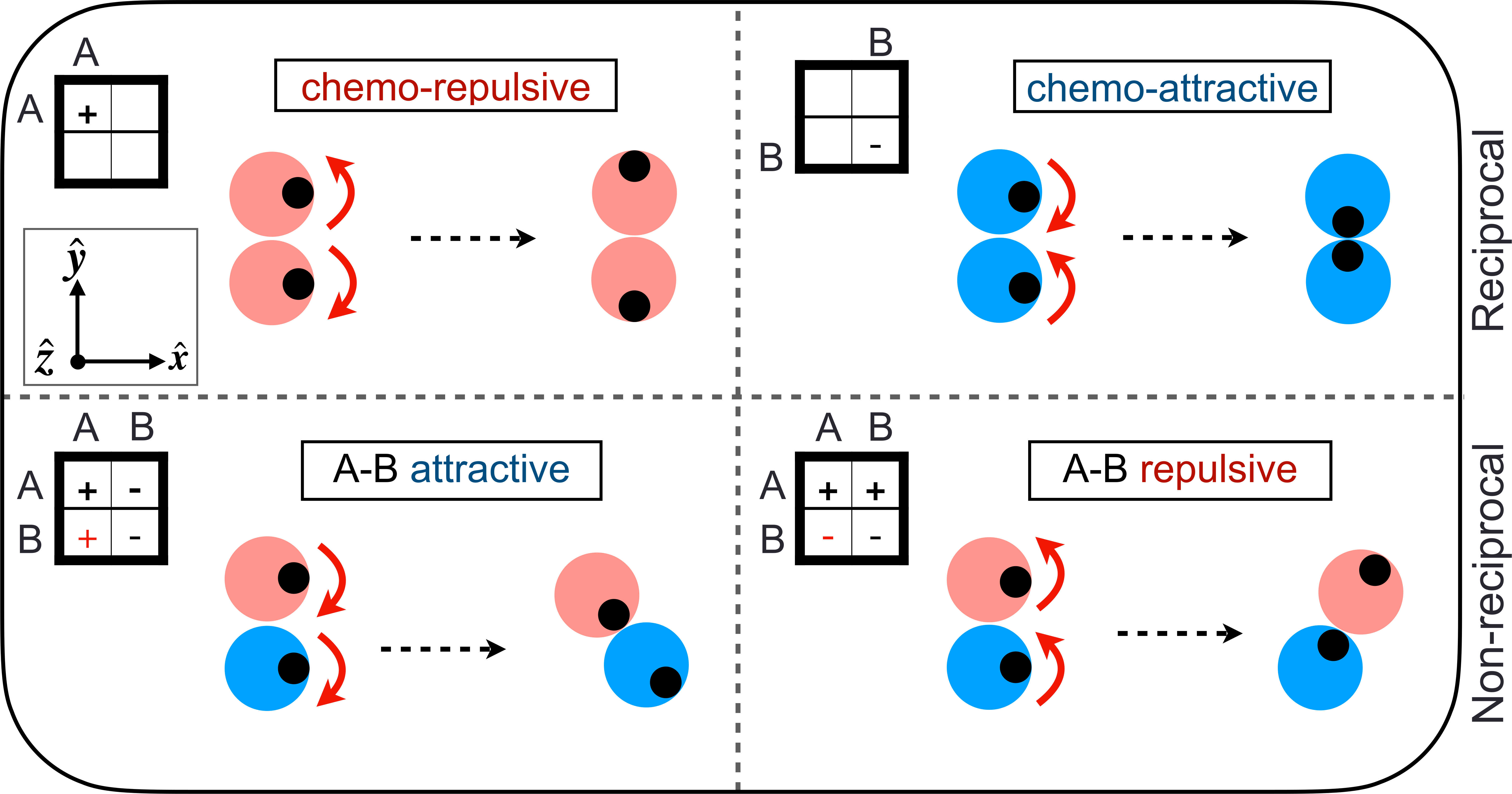
Figure 1: Schematic diagram for chemical interaction of a dimer. Two species of A type (red color) are purely repulsive, while those of B type (blue color) are purely attractive. The monomers are free to rotate and slide on each other, while the distance between the monomers does not change because of an inherent harmonic potential. So for repulsive interactions, they point away from each other, while they point towards each other for attractive interaction. For a dimer of both A and B types, the interactions are non-reciprocal. There are two choices: A attracts B and B is repelled away from A and vice-versa. The black dot indicate the orientation of the particles, while curved red arrows show rotations.

The rest of the paper is organized as follows. In Section II, we introduce our model of the chemically interacting chain of active Brownian particles, and specify important length and time scales, as well as dimensionless parameters that arise. In Section III, we discuss the chemo-repulsive case. We first outline our theoretical approach used in this problem, where we exploit the spatial symmetries of the chain to obtain the orientational fixed points and reduce the effective dimensionality of the problem. Then, we present results for the chemo-repulsive case, where we quantify both positional and angular rigidity of the chain. In Section IV, we present results for the chemo-attractive case, where we report collapsed crystalline lattices that (effectively) come to a halt. In Section V, we present results for the dimer and trimer cases, where we extend the system to a bidisperse one, and thus, allowing for the interactions between the monomers to be non-reciprocal. The result of non-reciprocity gives rise to novel collective phenomenon such as undulatory motion and reversal of direction of motion. Finally, in Section VI, we discuss our findings in relation to other work and discuss potential future work and applications.

II Model

II.1 Equations of motion

We model the $i$th active particle as a colloid particle centered at $\mathbf{r}_{i}$, confined to move in two-dimensions, which self-propels with a speed $v_{s}$, along the directions $\mathbf{e}_{i}=(\cos\theta_{i},\,\sin\theta_{i})$. Here $i=1,2,3,\dots,N$. The direction of the $i$th particle, given by the angle $\theta_{i}$, changes due to coupling to a phoretic field $c$. The position and orientation of the $i$th particle is updated as:

$$\frac{d\mathbf{r}_{i}}{dt}={\mathbf{V}}_{i},\qquad\frac{d\mathbf{e}_{i}}{dt}={\mathbf{\Omega}}_{i}\times\mathbf{e}_{i}.$$ (1)

Here, the translational velocity $\mathbf{V}_{i}$ and angular velocity $\mathbf{\Omega}_{i}$ of the $i$th particle are given as:

$${\mathbf{V}}_{i} =v_{s}\mathbf{e}_{i}+\mu\mathbf{F}_{i}+\sqrt{2D_{t}}\,\bm{\xi}^{T}_{i},$$ (2a)

$$\mathbf{\Omega}_{i} =\chi_{r}\left(\mathbf{e}_{i}\times\mathbf{\mathbf{{J}}}_{i}\right)+\sqrt{2D_{r}}\,\bm{\xi}^{R}_{i}.$$ (2b)

In the above, $\mu$ is mobility, $D_{t}$ and $D_{r}$, are respectively, translational and rotational diffusion constants of the particle, while $\bm{\xi}_{i}^{T}$ and $\bm{\xi}_{i}^{R}$ are white noises. As mentioned in Section I, variation of translational noise is naturally important when considering the statistical mechanics of long ‘conventional polymer(s)’; here we instead study the precise dynamics of these chains. Indeed, using experimentally feasible quantities of $b\sim 25~{}\mu$m, viscosity of solvent $\eta\sim 10^{-3}$ [22], we find that the typical active force [$\mathcal{O}(6\pi\eta bv_{s})\sim 10^{-11}N$], is dominant to the typical Brownian forces [$\mathcal{O}(k_{B}T/b)\sim 10^{-16}N$], thus for the rest of the paper $D_{t}$ is ignored. $D_{r}$ on the other hand, as we will show, plays a crucial role in the phase determination of the chain.

The chemical interactions in our model (2) drive orientational changes through the terms proportional to $\chi_{r}$. The case of $\chi_{r}<0$ (the chemo-attractive case) corresponding to monomers rotating towards each other, while $\chi_{r}>0$ (the chemo-repulsive case) implies that the particles rotate away from each other. This case corresponds to the well known mechanism of repulsion due to the trails of other monomers in the system [23, 24, 22]. The ‘translational chemotactic’ term (e.g. present in [24, 25, 26]) is not present in our model, as it does not alter the dynamics due to the presence of spring connections between the monomers of the chain. The force keeping the chain together is modelled as a spring. The force on the $i$th particle is given as: $\mathbf{F}_{i}=-\mathbf{\nabla}_{i}U$, while the potential $U$ is: $U=\sum_{i=1}^{N-1}U^{s}(\mathbf{r}_{i},\mathbf{r}_{i+1})+\sum_{i<j}U^{e}(\mathbf{r}_{i},\mathbf{r}_{j}).$ Here, $U^{s}=k\left(r_{ij}-2b\right)^{2}$ is spring potential of stiffness $k$ and natural length $2b$ which holds the chain together and only acts between neighbouring particles in the chain. $r_{ij}=|\mathbf{r}_{i}-\mathbf{r}_{j}|$ and $b$ is the radius of the monomers. $U^{e}$ is a repulsive potential precluding overlap of particles. We choose it to be also of the form $U^{e}=k^{e}\left(r_{ij}-2b\right)^{2}$ if $r_{ij}<2b$, while it vanishes otherwise. $k^{e}$ is a constant, which determines the strength of the repulsive force, which precludes overlap of particles. Note that there is no bending potential added. Thus, we expect the polymer to be highly flexible. We show below (section III) that chemical self-interaction leads to an emergent rigidity in the polymer.

The chemical interaction in Eq. (2) is contained in the term $\mathbf{\mathbf{\mathbf{{J}}}}_{i}$, which is given as:

$$\mathbf{\mathbf{\mathbf{{J}}}}_{i}(t)=-\left[\mathbf{\nabla}c(\mathbf{r},t)\right]_{\mathbf{r}=\mathbf{r}_{i}}$$ (3)

where $c(\mathbf{r},t)$ is the concentration of filled micelles at the location $\mathbf{r}$ at time $t$. In our model, where each particle is considered as a point source of chemicals, the dynamics of the field $c$ follows from the equation:

$$\frac{\partial c(\mathbf{r},t)}{\partial t}=D_{c}\nabla^{2}c(\mathbf{r},t)+\sum_{i=1}^{N}c_{0}\,\delta(\mathbf{r}-\mathbf{r}_{i}).$$ (4)

Here $D_{c}$ is the diffusion coefficient of the filled micelles, $c_{0}$ is emission constant of the micelles, and $N$ is the number of monomers in the chain. It should be noted that we model the particle as a point emitter of chemicals. Using the above, we can solve for $\mathbf{\mathbf{\mathbf{{J}}}}_{i}(t)$ as:

$$\mathbf{J}_{i}(t)=\frac{c_{0}}{\pi b}\sum_{\begin{subarray}{c}j=1\end{subarray}}^{N}\left[\Upsilon_{ij}\int\limits^{t-t_{0}}_{0}dt^{\prime}\frac{\mathbf{r}_{i}(t)-\mathbf{r}_{j}(t^{\prime})}{\mathcal{D}^{2}}{\mathcal{F}_{ij}(t,t^{\prime})}\right].$$ (5)

Here ${\mathcal{F}_{ij}(t,t^{\prime})}$ = $\exp\left(-[\mathbf{r}_{i}(t)-\mathbf{r}_{j}(t^{\prime})]^{2}/\mathcal{D}\right)$ and $\mathcal{D}=4D_{c}|t-t^{\prime}|$, while $t_{0}$ is a finite time delay between the chemical being released and sensed, which preempts any divergence in the mathematical form of $\mathbf{J}_{i}(t)$ [26]. In simulations, we choose $t_{0}$ to be much smaller than any other time-scale in the problem. The tensor $\mathbf{\Upsilon}$ contains our choice of chemical affinities. We explain our choice of non-reciprocal affinities in Section (V) below. This model was previously used in a recent work [22] to capture experimental phenomenology in a Hele-Shaw cell with monomers having chemo-repulsive interactions. In this work, we study monomers with both chemo-attractive and chemo-repulsive interactions. We also allow for monomers of different kinds in the same chain, and thus, study non-reciprocal chemical self-interactions in an active chain (see Figure 1).

We simulate Eq. (1) using a forward Euler-Maruyama method to evolve the positions and orientations of the particles in time with the parameters listed in appendix A, unless otherwise stated.

II.2 Length and time scales

We will now define some length scales and time scales that arise from this model. The basic length scale here is the monomer radius, $b$. This amounts to an additional length scale imposed on the problem (imposed via excluded volume repulsion) that do not appear in Eq. (1) and (2). This is contrasted with ”natural” length scales, that arise from non-dimensionalizing the equations of motion. There are two natural length scales:

$$l_{c}=\frac{D_{c}}{v_{s}},\quad l_{r}=\frac{\chi_{r}}{b^{2}D_{r}}.$$ (6)

$l_{c}$ gives the characteristic distance at which the chemical (i.e filled micelles) diffuses across the system, whilst $l_{r}$ gives the characteristic amount by which monomers change their orientation in response to the chemical fields (as opposed to spontaneously, which is simply $b$). There are four time scales , they are:

$$\tau=\frac{b}{v_{s}},\,\,\,\,\,\,\tau_{r}=\frac{1}{D_{r}},\,\,\,\,\,\,\tau_{f}=\frac{b^{3}}{\chi_{r}},\,\,\,\,\,\,\tau_{c}=\frac{b^{2}}{D_{c}}.$$ (7)

Here, $\tau$ is a spontaneous propulsion time scale, which is the time it takes for an isolated particle to move a distance equalling its radius in absence of any reorientation, $\tau_{r}$ is the time at which orientations turn randomly due to noise, $\tau_{f}$ is a deterministic time during which the orientations change in response to the chemical field, and $\tau_{c}$ is the time scale at which chemicals diffuse across the system.

II.3 Dimensionless parameters

Let us define two dimensionless activity parameters which we will use for the study:

$$\mathcal{A}_{1} =\frac{bv_{s}}{D_{c}}=\frac{b}{l_{d}}=\frac{\tau_{c}}{\tau},\qquad\mathcal{A}_{2} =\frac{\chi_{r}}{b^{3}D_{r}}=\frac{l_{r}}{b}=\frac{\tau_{r}}{\tau_{f}}.$$ (8)

Here we have used equations (6) and (7). $\mathcal{A}_{1}$ captures the relative effect of spontaneous propulsion versus diffusion of filled micelles in the system, which in turn induces the deterministic rotation. Intuitively, for a sufficiently large $\mathcal{A}_{1}$ the monomers evade the diffusing chemicals and no chemically-induced self-orgnanization will be possible, whereas below a threshold, the sufficient chemicals are diffused in the system such that the chemical contribution is evident. We will later see in Sections III and IV that this intuition is reproduced in the simulations. $\mathcal{A}_{2}$ on the other hand captures the relative contribution of deterministic versus random rotations of the orientations. The relative contributions of these various length and time scales, where appropriate, will be discussed in the context of the qualitative behaviour of the chain, in Sections III when discussing the phase diagram .

II.4 Initial conditions and measurable quantities

For the entire paper (unless specified otherwise) we use the following initial conditions:

$$\theta_{i}(0) =0,\qquad\qquad\qquad x_{i}=0,\qquad\forall i$$ (9a)

$$y_{i+1}(0) =y_{i}(0)+2b,\qquad\,1\leq i\leq N-1$$ (9b)

Here $\theta_{i}$ angle made by the orientation $\mathbf{e}_{i}$ of the $i$th particle with the $x$-axis. Thus, Eq.(9) implies that the initial chain is aligned vertically (upward facing in the plane of the page in this paper). In addition, we have observed that the results are somewhat universal and do not depend on the initial orientations (see SI [29]). A detailed study of the effect of initial conditions is not performed in this work.

Let us define some quantities we will use to characterize the dynamics of the chain. The speed of the chain can be studied by considering motion in the center of the mass (CM) frame of the references. We define the centre of the mass coordinate $\mathbf{R}$ as:

$$\mathbf{R}=\frac{1}{N}\sum_{i=1}^{N}\mathbf{r}_{i}.$$ (10)

It will be useful to decompose the dynamics into mutually perpendicular components. For this, we can define a polarization vector $\mathbf{P}$ as:

$$\mathbf{P}=\frac{1}{N}\sum_{i=1}^{N}\mathbf{e}_{i}.$$ (11)

Thus, we can define velocity components parallel to the chain alignment as: $\dot{r}_{i}^{\parallel}=\dot{\mathbf{r}}_{i}\cdot\mathbf{P}$. For reasons that will be apparent later, we further define the average speed of the chain in this case as:

$$u=\langle\dot{R}^{\parallel}\rangle_{\text{ss}},\qquad\dot{R}^{\parallel}=\frac{1}{N}\sum_{i=1}\dot{r}_{i}^{\parallel}$$ (12)

Here $\langle\dots\rangle_{\text{ss}}$ implies that the average is taken in the steady-state. Finally, the dynamics can be also characterized by MSD (mean-squared displacement) and MSAD (mean-squared angular displacements), which are defined as:

$$\text{MSD}(t) =\left\langle[\mathbf{r}_{i}(t)-\mathbf{r}_{i}(0)]^{2}\right\rangle$$ (13a)

$$\text{MSAD}(t) =\left\langle[\theta_{i}(t)-\theta_{i}(0)]^{2}\right\rangle$$ (13b)

where $\langle\dots\rangle$ denotes averaging over the monomers.

III An active chain of chemo-repulsive monomers

We first study a chain made of only one kind of monomers, which are chemo-repulsive in nature. The $\Upsilon$ matrix here has the form $\Upsilon_{ij}=1\quad\forall i\neq j$. We study the phase behaviour of the system as a function of $\mathcal{A}_{1}$ and $\mathcal{A}_{2}$. We note that, throughout the paper, we vary $\mathcal{A}_{1}$ by varying $D_{c}$ at a fixed $v_{s}$, whilst we vary $\mathcal{A}_{2}$ by varying $D_{r}$ at a fixed $\chi_{r}$. Our results for a chain made of chemo-repulsive monomers are summarized in the the phase diagram of Fig. (2), delimited by the curvature of the steady state chain. We quantify the curvature of the polymer chain via the Monge representation [30]. In particular, we compute $\kappa$ = $\left\langle\nabla\cdot\left[{\nabla h_{i}}/{\sqrt{1+|\nabla h_{i}|^{2}}}\right]\right\rangle$ where $h_{i}$ is the height function of the chain, evaluated at each monomer location, measured from the vertical line connecting the edge monomers. As above, the average is performed across the monomers in the chain, giving a scalar value. In our case, the inner bracket is simply reduced to $\partial_{y}\left[{\partial_{y}x_{i}(y)}/{\sqrt{1+|\partial_{y}x_{i}|^{2}}}\right]$.

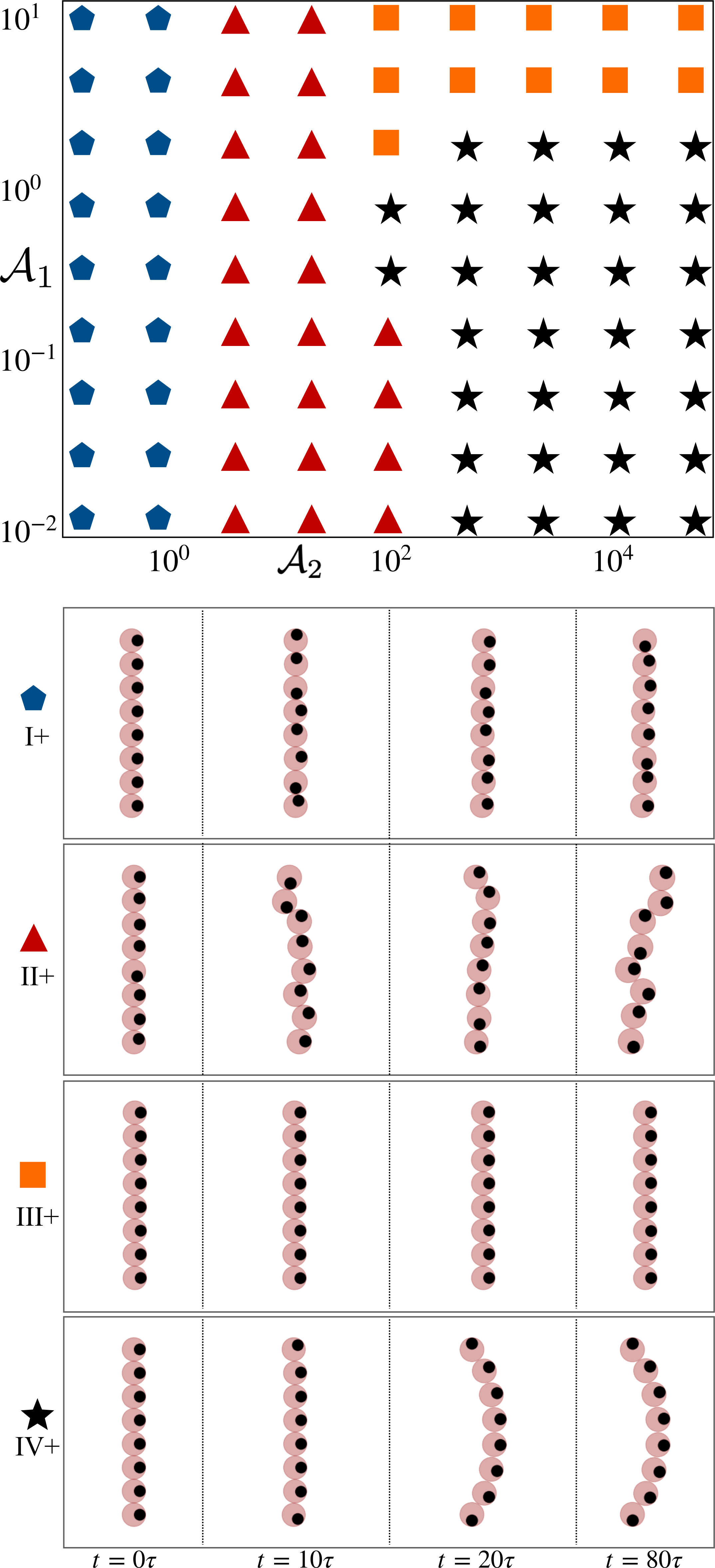
Figure 2: Phase diagram for the chemo-repulsive case. The top panel shows the phase diagram in the $\mathcal{A}_{1}$- $\mathcal{A}_{2}$ plane. The remaining panels show representative configuration from each distinct phase: (i) I+: Stiff + stationary chain, (ii) II+: Floppy chain (FLC-like dynamics), (iii) III+: Stiff+propelling state, (iv) rigid chain, self-propelling with C-shape. Parameters used for $(\mathcal{A}_{1},\mathcal{A}_{2})$ are (i) $(10^{-1},10^{-1})$, (ii) $(\mathcal{A}_{1},\mathcal{A}_{2})$ are (i) $(10^{1},10^{-1})$, (iii) $(10^{3},10^{1})$, (iv) $(10^{4},10^{-1})$. Phase diagram is constructed for $N=8$.

III.1 Results : Phase diagram

We now describe the phases displayed in phase diagram of Fig. (2). Region I+ corresponds to a stiff-noisy chain (see Fig. (2)) blue symbol, also bottom panel top row). This is defined by a rapid $\tau_{r}$ with respect to $\tau_{f}$, where $\frac{\tau_{r}}{\tau_{f}}=\mathcal{A}_{2}<<1$. In this region, we also have that $\frac{l_{r}}{b}=\mathcal{A}_{2}<<1$ (thus distances where the chain could potentially fold are negligible compared to the monomer radius). Note also that in this region $\tau_{r}/\tau_{f}\sim\mathcal{O}(10^{-3}-10^{-1})<<\tau/\tau_{f}\sim\mathcal{O}(1)$, thus the chain orientations fluctuate much quicker than they can pick up a direction of motion. Increasing $\mathcal{A}_{2}$, we arrive at Region II+, which corresponds to a quasi-FJC (freely jointed chain) region, shown in Fig. (2), red symbol. Here, the chain translationally diffuses, but folds into and out of a given configuration (see Fig. (2) bottom panel second to top row). In this region we have that $\mathcal{A}_{2}\sim\mathcal{O}(10^{0}-10^{2})$, i.e. the diffusive ($\tau_{r}$) and deterministic ($\tau_{f}$) impart equal contributions of deterministic and diffusive rotational motion - resulting in the motion qualitatively resembling a freely-jointed chain [19]. Region III+ is denoted in Fig. (2) with the yellow squares. This is the under-diffuse region, where the chain propels deterministically, but does not fold (see Fig. (2), bottom panel second to bottom row). Here, we have that $\frac{\tau_{c}}{\tau}=\mathcal{A}_{1}^{-1}<<1$, thus the chemical diffuses much slower that the spontaneous propulsion time, and equally $\frac{l_{d}}{b}=\mathcal{A}_{1}^{-1}<<1$. Finally, region IV+, denoted with black symbols in Fig. (2), is the C-shape region, where the polymer propels deterministically and self-organizes into a stable configuration that resembles the alphabet C [22, 11] (see Fig. (2), bottom panel bottom row) . We have that $\frac{\tau_{r}}{\tau_{f}}>>1$ (diffusive rotational time is negligible), $\tau_{r}\sim\tau$ (both deterministic rotation and propulsion occur simultaneously), and $\frac{l_{d}}{b}>>1$.

The characteristic dynamics of each region is shown in Fig. (2) (bottom panel). After $t=10\tau$, we see that the orientational changes in the chain have set in. The dominant time scales here are $\tau_{r}$ for noise-dominated phases I+ and II+, whereas for phase IV+ $\tau_{f}$ is dominant, with deterministic alignments seen. After $t\sim 20\tau$, we see that in phase IV+ steady-state spatial structures have formed, namely an acquisition of curvature to form a C-shape, which is identical at $t=80\tau$. For such deterministic changes to occur we note that the history dependence of the dynamics (c.f. Eq. (5)) is necessary. In other words, chemicals that are built-up from previous times $t^{\prime}<t$ drive the dynamics at time $t$. Naturally, this requires $\tau_{c}$ to be much smaller than other deterministic time scales $\tau$ and $\tau_{f}$, which is the case in phase IV+. In the absence of such a dominant $\tau_{c}$ - there is no historical buildup of the chemicals - we get phase III+, no interactions occur. This history-dependence of the dynamics distinguishes this model (see also [26, 24]), from other chemically interacting colloidal models [31, 32, 33, 25] , where instantaneous chemicals are assumed to be deposited on the surface.

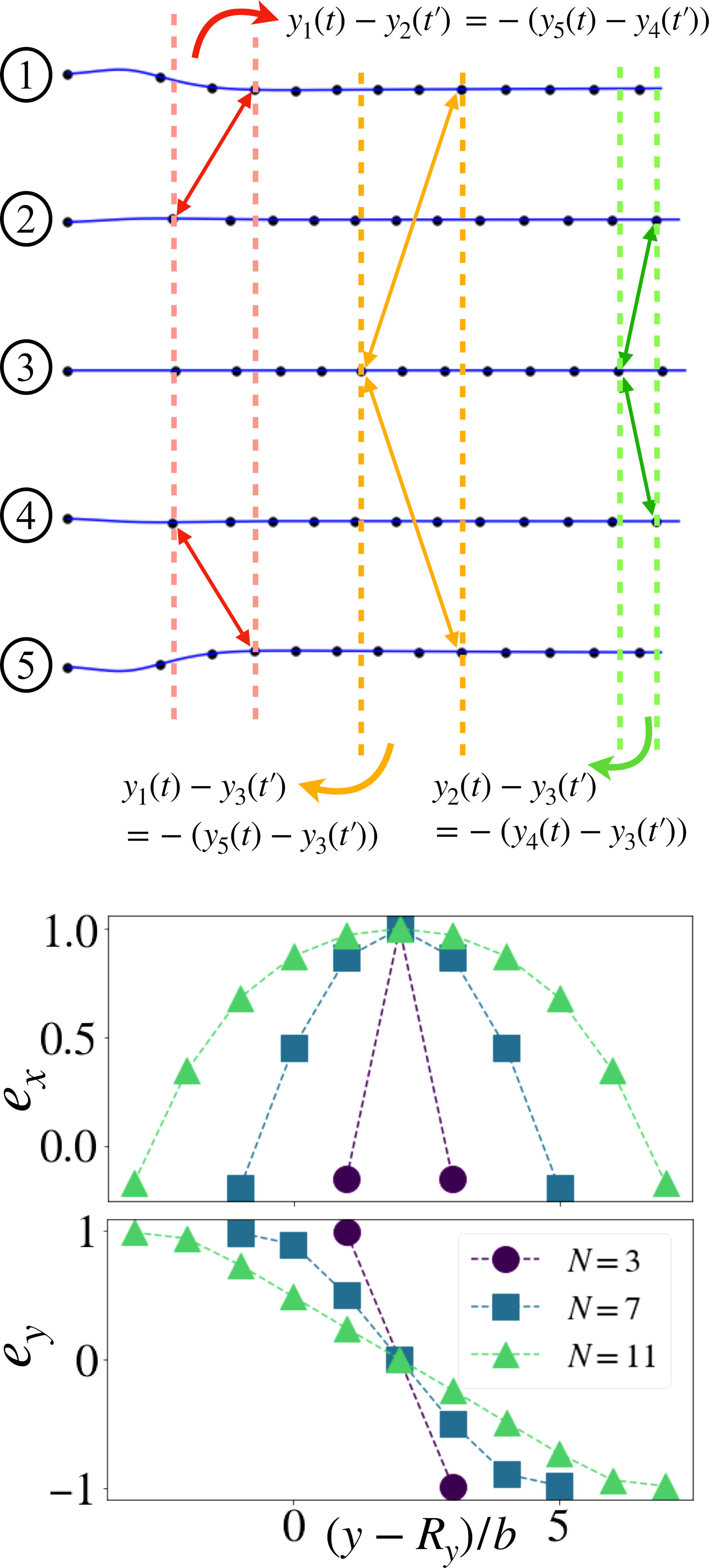
Figure 3: Illustration of the symmetry of the dynamics for the chemo-repulsive case of $N=5$. TOP PANEL: trajectory of each monomer in the chain is shown (labelled on the left), with time points colored in black. The equalities in (15) can be deduced by taking vertical distances at different time points (a particular $(t,t^{\prime})$ pair is uniquely coloured). Equalities of (16) is deduced by considering the time spacings. BOTTOM PANEL: steady-state orientations ($e_{x}$ and $e_{y}$) satisfying Eq. (18) are shown, for $N=3$, $N=7$, and $N=11$. Dotted lines are a guide to the eye.

III.2 Theoretical approach to dimensionality reduction

We further study phase IV+, specifically the noiseless case. To do this, we will employ a theoretical approach that exploits the symmetries of the dynamics of the monomers along the chain, from which we will reduce the dimensionality of our 3N degrees of freedom and define coarse-grained quantities. The result of this procedure yields the following equation

$$u=v_{s}|\mathbf{P}|$$ (14)

which is thus a linear relationship between time-averaged quantity $u$ and an order parameter $\mathbf{P}$ of this $3N$ dimensional system. Thus, although a linear relation akin to (14) is applicable at all times (using the instantaneous velocity instead of the time-average), the above is a unique specific case, relating a time-averaged dynamical quantity to an order parameter of the system. This is possible due to the symmetry of the dynamics.

To prove Eq.(14), as an instructive case, let us consider the time trajectory of the $N=5$ chain, shown in Fig. (3)(a) (see Appendix B). The dynamics can be seen to be fully symmetric about the central monomer, and the following equalities can be deduced

$$y_{1}(t)-y_{2}(t^{\prime}) =y_{4}(t^{\prime})-y_{5}(t)$$ (15a)

$$y_{1}(t)-y_{3}(t^{\prime}) =y_{3}(t^{\prime})-y_{5}(t)$$ (15b)

$$y_{2}(t)-y_{3}(t^{\prime}) =y_{5}(t^{\prime})-y_{4}(t)$$ (15c)

and further

$$x_{1}(t)=x_{5}(t),\quad x_{2}(t)=x_{4}(t),\quad\forall t$$ (16)

This symmetry, as we show in Appendix (B), allows us to show that the fixed points of the orientations are symmetric in one and anti-symmetric in another direction:

$$e_{x_{1}} =e_{x_{5}},\quad e_{y_{1}}=-e_{y_{5}}$$ (17a)

$$e_{x_{2}} =e_{x_{4}},\quad e_{y_{2}}=-e_{y_{4}}$$ (17b)

$$e_{x_{3}} =1,\qquad e_{y_{3}}=0$$ (17c)

For an arbitrary chain of N monomers, this generalizes to the condition:

$$e_{x_{i}}=e_{x_{N-i+1}},\quad e_{y_{i}}=-e_{y_{N-i+1}},\quad\forall i\in\{1,2,...,N\}$$ (18)

Thus, a spatial symmetry in the problem implies an orientational symmetry. Note also that for odd-numbered chains, (18) implies that $(e_{x},e_{y})=(1,0)$ for the monomers in the (arithmetic) center (see Appendix (B). This symmetry is shown in Fig. (3b), where the orientations are plotted in the CM frame perpendicular to the propagation direction, in the continuum parametrization, showing that $e_{x}(y-R_{y})=e_{x}(-(y-R_{y}))$, (top panel) and $e_{y}(y-R_{y})=-e_{y}(-(y-R_{y}))$ (bottom panel) (the relation between the two given straightforwardly by $e_{y}=\sqrt{1-e_{x}^{2}}$). Note that this straightforwardly implies that $\theta(y-)=-\theta(-(y-R_{y}))$. Summing up Eq. (1) across the chain, and using Eq. (11), we obtain Eq. (14).

We will show, in this and the following sections, that the scaling of Eq. (14) holds true whenever the symmetries in (15) and (16) are applicable (for example, during a certain duration of the dynamics). We will also show in Sections (V) that these symmetries can effectively reduce the dimensionality of the system for dimer and (selected) trimer configurations. We also note that this scaling also holds true for arbitrary initial conditions not given by Eq. (9) [22]. In this case, (14) does not apply throughout the dynamics, but merely in the steady-state, when the chain acquires the C shape (irrespective of the initial condition) that characterizes in phase IV+.

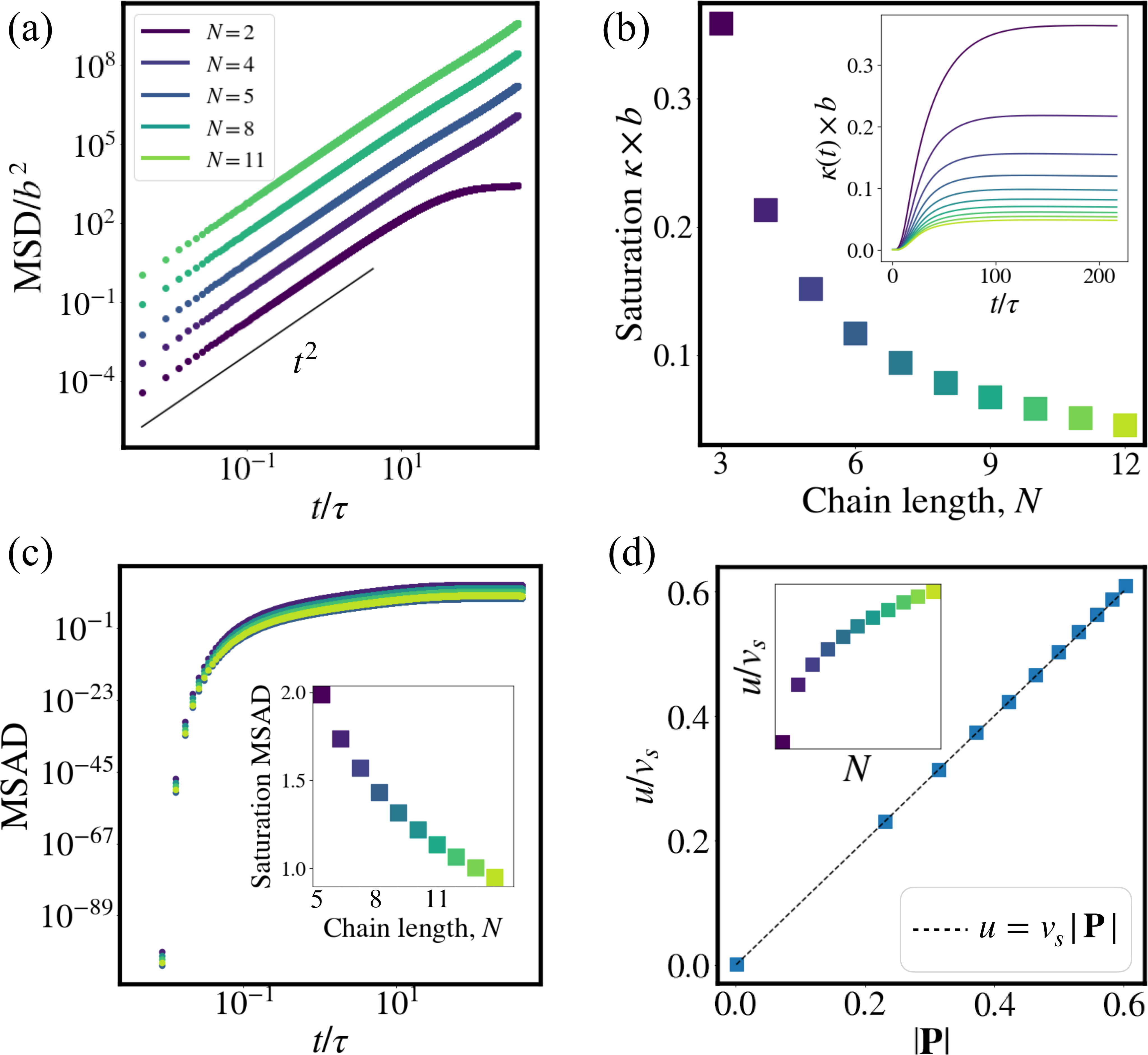
Figure 4: Results for chemo-repulsive - Phase IV+. In panel (a), the ballistic nature of the polymers are captured via the MSD ($N=2$, $4$, $5$, $8$, and $11$ shown), for all except the dimer where the motion stops (see section V.1). Note that the lines are vertically adjusted such that there is spacing in between for distinguishability. In (b) the saturation value of curvature ($\kappa$) of the chains are shown, with the time evolution in the inset. Note that colors in the inset match that of main figure. The saturation $\kappa$ behavior is indicative of the fact that in the continuum limit the curvature of a generalized ellipse is a constant. Thus, the larger chains are more ”rigid”. In (c), the MSAD of the chains are shown. In the inset the saturation value is displayed, indicating now an ”angular stiffening” of the chain with $N$. In panel (d) relation (14) is verified, whilst in the inset its value with $N$ is shown. Thus, longer chains that are stiffer eventually also converge to a steady-state propulsion speed. Note that color bars across all panels (here and in other figures throughout the paper) are identical.

III.3 Phase IV+ : Results

In the stable phase, we further study its dynamics and steady state properties of the C-shape. We see in Fig. (4a) that the chain propels ballistically, $\text{MSD}\propto t^{2}$ for all values of $N\geq 3$. We note that for $N=2$ the chain stops, this will be explained in the Section V below. The positional stiffness of the chain is quantified by curvature ($\kappa$) in Fig. (4b). We see that for longer chains $\kappa$ decreases and eventually saturates to a finite value, indicating ”stiffer” longer chains. In the inset, we see that the initially stiff chain acquires a curvature throughout the dynamics, saturating at a particular value after $\sim 10^{2}s$. Further, the angular stiffness is quantified by the MSAD in Fig. (3c), which also saturates. The saturation MSAD (inset) shows a similar decrease w.r.t $N$, indicating that longer chains are more ”angularly stiff” in that they deviate less from $\theta_{i}(0)$ throughout the dynamics. Finally, we have $u/v_{s}$ versus $|\mathbf{P}|$ where we have a relation as predicted by Eq. (14), validating our dimensionality reduction procedure. In the inset we see that the $u/v_{s}$ also saturates in the continuum limit, corresponding to a saturation of $\mathbf{P}$ in this limit.

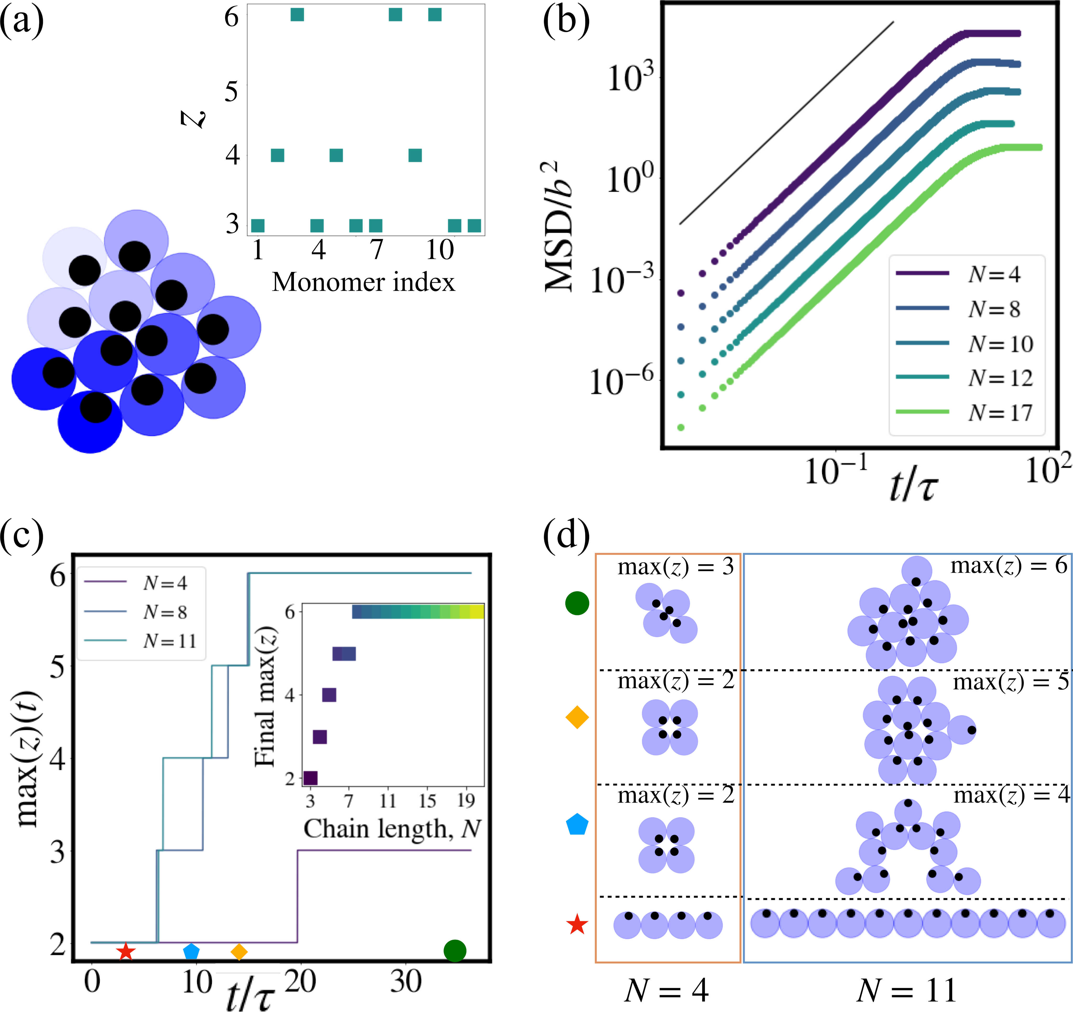
Figure 5: Chemo-attractive results: distinguishing metastable and hexagonally packed states. Panel (a) displays an example of a hexagonally-packed crystal. The colors are shaded such according to monomer number starting from the vertically most upward being the lightest. The coordination number for the configuration is shown in the inset, with the central three ($z=6$), edge ($z=4$) and vertex ($z=3$) monomers displayed. In (b), the MSD in plotted (for $N=4,8,10,12,\text{and}17$), where the halting of motion is seen at $t\sim 10\tau$. In (c), examples of the time evolution of our packing order parameter $\max(z)(t)$ is shown for $N=4$,$8$, and $11$, to distinguish between metastable the lattice of $N=4$ and the remaining two hexagonal packing. The former has a long lived transient lasting $O(10^{1})\tau$, whilst the latter has much short-lived transients, eventually reaching $\max(z)=6$. In the inset, the final value is shown, showing that $\max(z)=6$ is attained from $N=8$ onwards. For the time points labelled in the bottom of (c), the snapshots of the packing are displayed in (d), for $N=4$ (left) and $N=11$ (right). In particular, the final packed crystals have no positional spacing in between next-no-nearest neighbouring monomers, which can be seen for $N=4$ of the first and second from bottom rows, and $N=11$ for the first from bottom row.

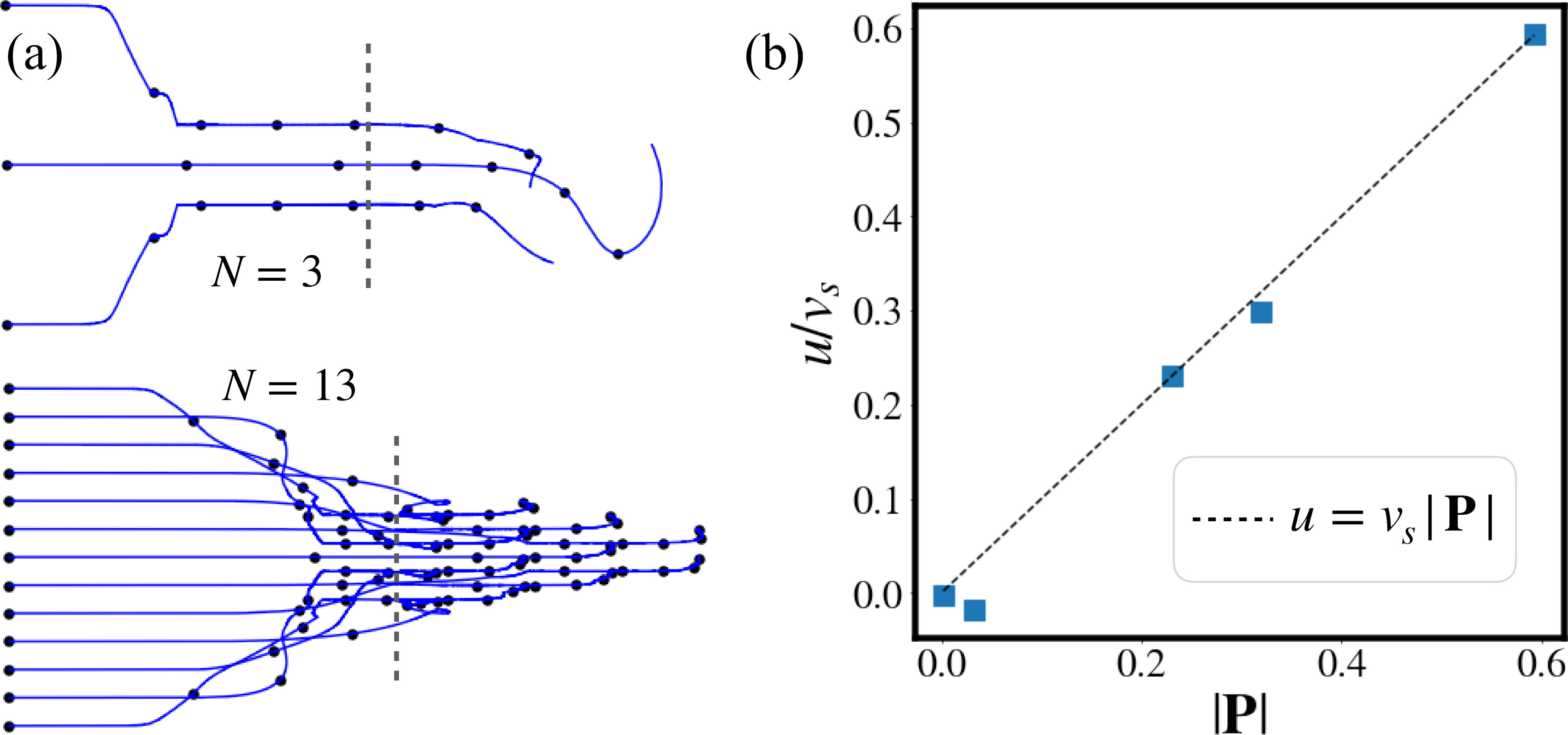
Figure 6: Metastable lattices in the chemo-attractive case, demonstrating range of validity of the symmetric-trails approach. In (a) top, we see that the symmetry holds for the metastable transient up to the collapse time (vertical dotted line), thus the averaging in (12) is performed for time points in the metastable state suitably before. On the bottom panel, we show that, even without a metastable lattice, hexagonally packed lattices also display such a symmetry. In (b), $u$ vs. $|\mathbf{P}|$ is shown for the metastable lattices ($N=3$,$4$,$5$,$6$, and $7$), showing a good agreement with (14).

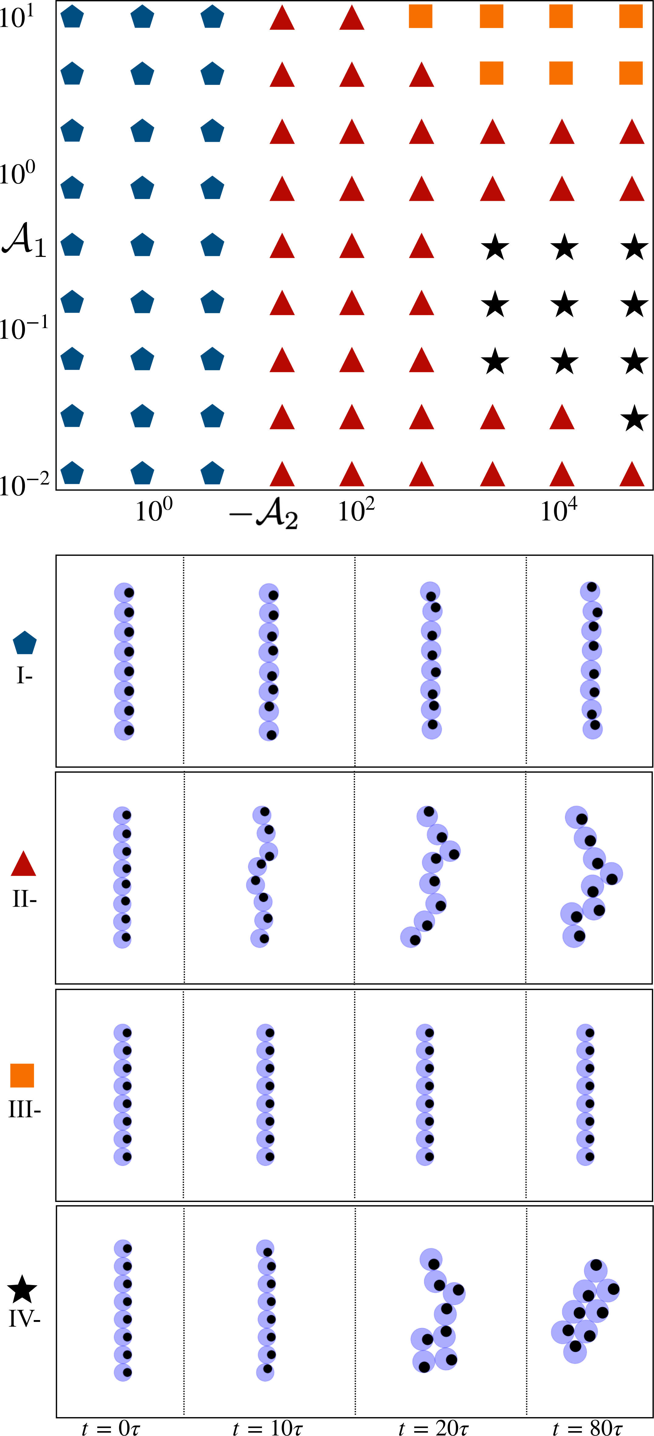
Figure 7: Phase diagram for the chemo-attractive case. The four states are: (i) I-: Stiff + stationary chain, (ii) II-: FLC-like dynamics, (iii) III-Stiff+propelling state, (iv) IV-: closed packed lattice. Parameters used for $(\mathcal{A}_{1},\mathcal{A}_{2})$ are (i) $(10^{-1},10^{-1})$, (ii) $(\mathcal{A}_{1},\mathcal{A}_{2})$ are (i) $(10^{1},10^{-1})$, (iii) $(10^{3},10^{1})$, (iv) $(10^{4},10^{-1})$. Phase diagram is constructed for $N=8$.

IV An active chain of chemo-attractive monomers

We now turn to the case of chemo-attractive monomers with $\chi_{r}<0$. The $\Upsilon$ matrix here has the form $\Upsilon_{ij}=-1\quad\forall i\neq j$. Here, the monomers will preferentially point towards each other upon sensing the chemical field. We report a novel colloidal crystallization mechanism [34, 1, 35, 8] where the long-ranged attraction renders the initially propelling chain to undergoes a collapse onto itself thereafter remaining quasi-stationary (see SI Movie [29]).

IV.1 Metastable crystallites for $N<8$

We first distinguish two separate cases of collapsed chains, which we call (i) metastable crystallites, and (ii) hexagonally packed crystals. The former is characterized by long-lived (typically $\sim 10^{1}-10^{2}\tau$) transient metastable crystals (either propelling or stationary depending on net $\mathbf{P}$) that collapse onto other crystal within the time scale of simulation, whilst the latter is does not display any such transient states (any transients further collapse within O($\tau$)).

To distinguish these two types of crystals, we define a coordination number ($z$) for each monomer

$$z=\{|\mathcal{N}_{i}|,\forall i\},\qquad\mathcal{N}=\{|\mathbf{r}_{i}-\mathbf{r}_{j}|<2b,\forall j\neq i\}$$ (19)

with the $\max(z)$ being an order parameter used to distinguish different steady-state configurations. For all chain lengths $N$, the steady-state crystals are close-packed structures, such that each monomer has $z\geq 2$. For chains of $N\geq 8$, this is identified by $\max(z)=6$ (hexagonal packing). For $N<8$, we in turn have the metastable crystallites. An example of this is shown in Fig. (5a), with the top panel displaying the packing evolution of the $N=4$ chain, whilst the bottom for $N=11$. For the former, we see that the metastable ”square” structure, with $\max(z)=3$, exists at times $t=10\tau$ and $t=13\tau$ (top panel second and third columns, eventually closing in further into a ”cone” structure, with $\max(z)=3$, at $t=35\tau$ (right column). This metastable crystal is captured via the time evolution of $\max(z(t))$ in Fig. (5c), with only only discrete change in $\max(z(t))$ seen, corresponding to the ”square”-to-”cone” transition. The behaviour for hexagonally packed crystals are markedly different, as is also seen in Figs. (5a) ($N=11$) and (5c) ($N=8$ and $N=11$). In particular, we see that any transient lattices do not last longer than a few $\tau$, before packing further into a more close-packed structure, eventually forming the crystal. An example for this for $N=11$ is shown in Fig. (2a) (bottom panel).

Note that in theory $N=7$ permits hexagonal packing, though in our simulations this occurs for selected realizations of noisy simulations ($D_{r}>0$), or with carefully selected initial conditions that deviate from (9). Thus, we do not study this hypothetical packed crystal any further.

Having made this distinction, let us study further analyse these metastable crystallites. Let us call the time at which there metastable crystallites lose their stability as the collapse time. We can again exploit the symmetric histories argument, which we find to be applicable up to the collapse time. This is displayed in Fig. (6a) (top row). A straightforward consequence of this is the applicability of relation Eq. (14) in this regime. This is displayed in Fig. (6b), where the average in (12) is performed for time points before the collapse time. Data points here correspond to hence only $N=3,4,5,6,7$ simulations. Beyond this regime, relation (14) is indeed no longer applicable. We note that for hexagonally packed crystals, $|\mathbf{P}|\sim 10^{-1}$ in this scaling regime, thus we do not display the data points in Fig. (6b), but they also agree with (12) within this regime.

IV.2 Hexagonal packing

For hexagonally packed crystals, there is also positional symmetry in the dynamics, as is displayed in Fig. (6)(bottom panel) for the case of $N=13$. However, we study instead the fully-packed structure, which is quantifiable by $z$. An example of this close-packed crystal is shown in Fig. (6d) for $N=13$. As a rule, either monomer on the edges of the initially straight configuration appear on the rim of the packed crystal. The specific set of $z$ for this $N=13$ configuration is shown in the inset, where the monomer set with $z=3$ correspond to those in the rim and part of a pair-vertex, the pairs being (in monomer index units) $(1,4)$, $(7,8)$, and $(11,12)$. Those with $z=4$ correspond to rim plus edge monomers, i.e neighbouring the vertex monomers on the same edge, whilst those with $z=6$ correspond to the inner monomers. Apart from that, the exact configuration of packing varies significantly with (among others) $\chi_{r}$. For instance, larger $\chi_{r}$ (thus larger $l_{r}$ that promotes folding stronger at the edges, since deterministic rotation dominates over longer length scales of the chain (versus propulsion) - see SI Movie [29]). We do not study any further the monomer distribution of the packed structure as a function of these parameters as part of this study.

The dynamics of these structures display quasi-halting of motion. The halting of the chain is seen via the MSD in Fig. (6), where a plateau is seen, which was absent in the chemo-repulsive case (with the exception of $N=2$). This occurs at $t\sim 10\tau$, corresponding to the point of $\max(z)=6$ in Fig. (6)(c). The net polarization of this packed lattice is found to be of $\sim 10^{-2}$, with $u$ of the final crystal at most $1/10$th the minimum $u$ of the chemo-repulsive case. Movies of various packing sequences are shown in SI [29].

IV.3 Phase diagram

We can repeat the same procedure as done in the previous section and obtain the phase diagram for the chemo-attractive system; here, we use $\max(z)$ (maximum coordination number) to distinguish the different phases. This is shown in Fig. (7). It is qualitatively similar to that in Fig. (2), and thus we have identically labelled the phases as I-, II-,III-, and IV-, where the aforementioned relative dominance of relevant length and time scales in each of the phases are identical. The region IV- differs from IV+ in that they now describe a collapsed lattice structure. Further, the line delimiting phases IV and II for large $\mathcal{A}_{1}$ (the over-diffuse region) if shifted, such that large $\mathcal{A}_{1}$ and large $\mathcal{A}_{2}$ (e.g. $(10^{3},10^{-2})$) does not crystallize. We expect that a similar trend to be seen for the chemo-repulsive case if values $\mathcal{A}_{1}<<10^{-2}$ are probed - i.e no stable C-configuration when the system is over-diffuse since there are no discernible concentration gradients in the system. Phases II+ and II- are also qualitatively different, in that in the latter case, one sees more distinct ”FJC-like” behaviour, with the chain collapsing and relapsing on itself (see SI Movie [29]), compared to II+ where there is no collapse as such. Rotational diffusion has previously been argued to drive crystal break-up and re-arrangement [34] in activity-driven aggregation [36, 1], and we see a chain analogue of this in this phase. In addition, we have also measured in the MSAD (not shown in this paper), where, unlike in the chemo-repulsive case, there is no stiffening with larger $N$, by reason of its collapsed configuration.

V An active chain with Binary mixture of chemo-attractive and chemo-repulsive monomers

We next turn our attention to a binary mixture system, where two species A and B populate the chain. We further focus on the case where the two-species interact in a non-reciprocal fashion, such that (for instance) A chases B, whilst B is repelled from A.

Such non-reciprocal interactions are known to be present in (isolated) colloidal systems [37, 38, 39, 40, 41], and have been studied theoretically and computationally in various particle-based [32, 33, 25]; field-theoretic [42, 43], and continuum solid [44, 45, 46] models. Our study here is distinct in that the non-reciprocity by itself does not drive the system out of equilibrium [33, 42, 43, 44], since the constituent units of our system are polar. We will observe a wide range of phenomenology, some of which are hitherto unreported in such systems.

We first study dimers of configurations AA,BB, and AB; and later proceed to the study of trimers. In the later case, we will show that the breaking of action-reaction symmetry in the monomer interactions lead to emergence of states that display features of oscillations and direction reversal. For the rest of this section, we will denote AB+(-) and that where species A is attracted to (repelled from) species B. For the entirety of this section, we study the noiseless case with sufficiently diffuse chemicals ($D_{r}=0$, with $\tau_{c}<<\tau$, i.e in the Phase IV regime of Figs (2) and (7)). A full study of the different phases for dimers and trimers are not carried out here, though we expect the results to be qualitatively similar to those in the previous section.

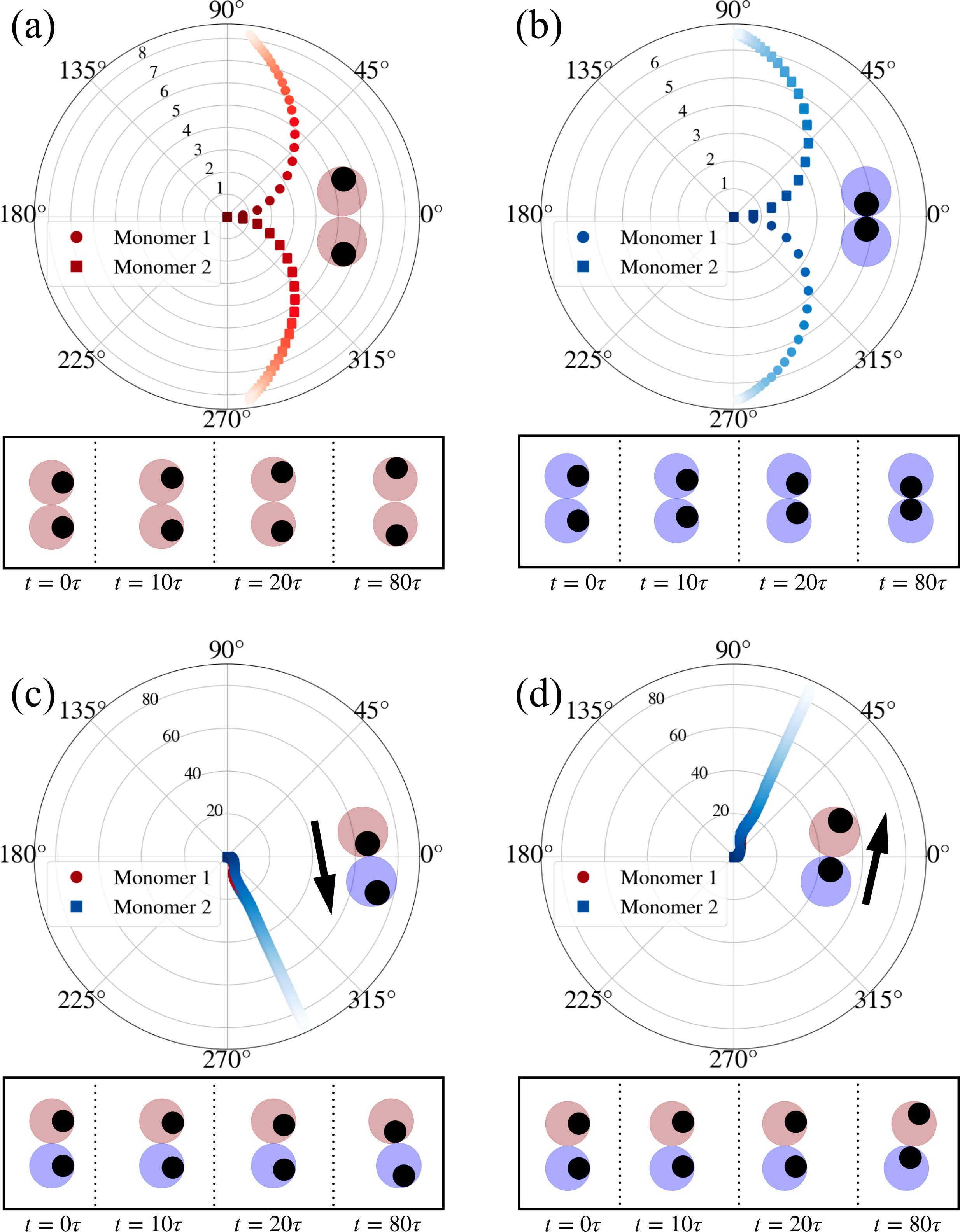
Figure 8: Dynamics of dimers for AA, BB and AB cases. Polar plots of the dynamics are displayed in panels (a) - (d). The radial axis of these plots indicate distance, $|\mathbf{R}_{i}(t)|/b=\sqrt{x_{i}(t)^{2}+y_{i}(t)^{2}}/b$, from the origin. The trajectories are color shaded according to time - from darkest (initial) to brightest (final). Inset indicates snapshot of steady-state dimer, with accompanying arrow showing its propulsion direction (no propulsion for AA and BB dimers in the steady-state). Each panels also displays snapshots at $t=0$, $10\tau$, $20\tau$, and $80\tau$.

V.1 Dimers - single species

For the single species dimers, we have shown in Fig. (4) previously that the dimers (AA) come to a halt (see SI video [29]). This is seen in the polar plot of Figure (8)(b), where we see the initially vertical orientations reach the fixed points for $\theta_{1}^{*}=\frac{\pi}{2}$ and $\theta_{2}^{*}=-\frac{\pi}{2}$. This is also true for the BB configuration; this is shown in Fig. (8)(a) (top row) and the polar plot of Fig. (8)(b), where now $\theta_{2}^{*}=\frac{\pi}{2}$ and $\theta_{1}^{*}=-\frac{\pi}{2}$ (see SI video [29]). The orientational fixed points are thus

$$\mathbf{e}_{1}^{*}=\Bigg{(}\begin{smallmatrix}0\\ \\ 1\end{smallmatrix}\Bigg{)},\quad\mathbf{e}_{2}^{*}=\Bigg{(}\begin{smallmatrix}0\\ \\ -1\end{smallmatrix}\Bigg{)}$$ (20)

which is directly implied by (18). For the BB configuration the fixed points are the opposite

$$\mathbf{e}_{1}^{*}=\Bigg{(}\begin{smallmatrix}0\\ \\ -1\end{smallmatrix}\Bigg{)},\quad\mathbf{e}_{2}^{*}=\Bigg{(}\begin{smallmatrix}0\\ \\ 1\end{smallmatrix}\Bigg{)}$$ (21)

with its dynamics displayed in Fig. (8)(a) (second row) and the polar plot of Fig. (8)(c). We see that the AA and BB configurations are completely symmetric to one another.

We can further use Eq. (20) to show that the dynamics of both AA and BB come to a halt. To do this, note that in the CM frame of motion, we have after adding Eq. (1) for both species,

$$\frac{d\sum_{i}\mathbf{r}_{i}}{dt}=v_{s}\sum_{i}\mathbf{e}^{*}_{i}+\mu\sum_{i}F_{i}=v_{s}=v_{s}\sum_{i}\mathbf{e}^{*}_{i}$$ (22)

In the above we have used that fact that for $N=2$, $\mathbf{{J}}_{1}=-\mathbf{{J}}_{2}$ (and for any $N$ the spring forces sum to zero). Thus,

$$\sum_{i}\mathbf{e}^{*}_{i}=0\implies\frac{d\mathbf{R}_{i}}{dt}=0.$$

So, we arrive at the result that the CM motion is static.

V.2 Dimers - AB

We now turn to the case of non-reciprocal dimers, where we uncover an ”alignment chasing” behaviour. Such two-species chasing has been reported in previous studies of colloidal models (far-field interaction with short ranged chemicals [32], field-theoretic models [42, 43], and prey-predator models [47, 48]. Thus, the alignment chasing reported here extends this phenomenon to an active colloidal polymer in a straightforward manner. For the dimer-AB, the matrix entries for $\Upsilon_{ij}$ are given by:

$$\Upsilon_{ij}^{AB}=-\delta_{i1}\delta_{j2}+(1-\delta_{i1}\delta_{j2})\delta_{i2}\delta_{j1}.$$ (23)

In addition, we use the notation (-)/(+) at the suffix of the configuration to denote whether the configurations have an attractive/repulsive AB interaction. Thus, it is clear that in the case of an AB-dimer, the action-reaction symmetry can be broken in two distinct ways [AB(+) and AB(-)]. We study both these cases below.

The results for the AB configuration are shown in for the AB- configuration in Figure (8c) and (8a)(third row), whilst the AB+ configuration is in (8d) and (8a)(bottom row), where we see that the monomers quickly settle on a solution where they are mutually aligned (having the same orientation) (see SI video [29]), for both AB+ and AB-.

This chasing result is also straightforwardly deduced analytically. Considering the attractive AB interaction, we have that the fixed point for $\dot{\mathbf{e}}_{1_{A}}=0\implies\mathbf{e}_{1_{A}}\propto-|\chi_{r}|(\mathbf{r}_{1_{A}}-\mathbf{r}_{2_{B}})$, whilst $\dot{\mathbf{e}}_{2_{B}}=0\implies\mathbf{e}_{2_{B}}=0\propto+|\chi_{r}|(\mathbf{r}_{2_{B}}-\mathbf{r}_{1_{A}})\quad/\!\!/\quad\mathbf{e}_{1_{A}}$. This happens after about $t\sim 80\tau$ of the dynamics (see Fig. (8)(a), bottom row.). On the other hand, the dynamics at the fixed point in the phase space of $\{R_{x},R_{y}\}$ read

$$\frac{dR_{x}}{dt}=2v_{s}\cos(\theta^{*}),\qquad\frac{dR_{y}}{dt}=2v_{s}\sin(\theta^{*})$$ (24)

after which the dimer propels indefinitely along a fixed angle $\theta^{*}$ which we can also deduce. The steady state angle the dimer picks is $\approx 292.5^{\circ}$, half way in between that of a full vertically downward chase ($\theta=270^{\circ})$, and an unbiased diagonal $\theta=315^{\circ}$, owing to the symmetry of the problem. For the AB(+) case, the same argument gives the steady-state angle as $\approx 67.5^{\circ}$.

Let us summarize the results for dimer interactions. The monodisperse dimers (both AA and BB) come to a halt, whereas the bidisperse dimers propel at a fixed angle, one species chasing the other indefinitely. The reduced phase space is 3 dimensional for the monodisperse dimers throughout the dynamics (see Appendix C). For the AB molecules, the reduced phase space is also 3 dimensional, where we can additionally show it to be stable, whilst it is 1 dimensional at the fixed point orientations, corresponding to a stably propelling dimer. With this, we now move on to the trimer cases.

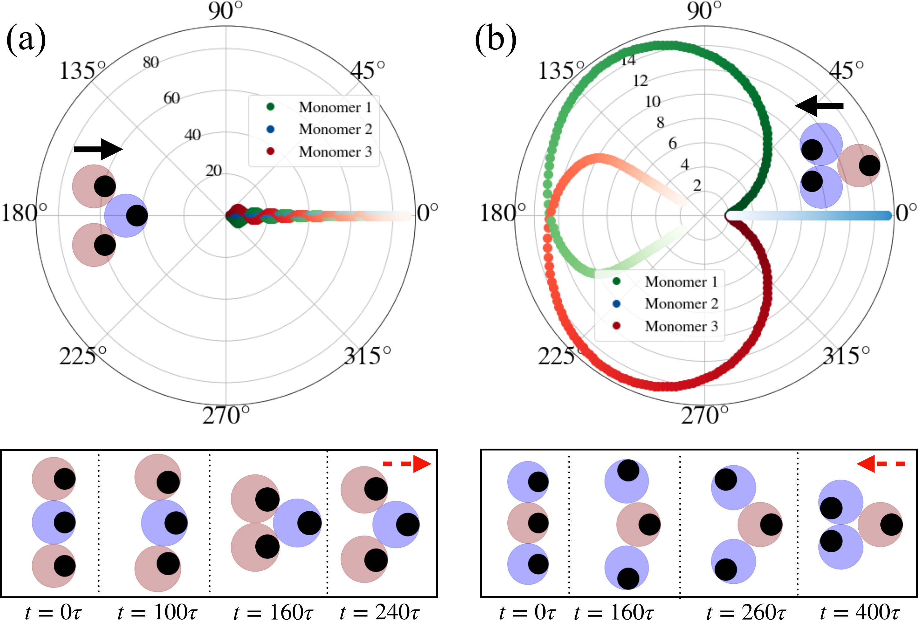
Figure 9: Dynamics of trimers, ABA(-) and BAB(-), with chemical affinities that break the action-reaction symmetry. Panels (a)-(b) on top row display polar plots for ABA(-), BAB(-) respectively. The bottom panels show the snapshots from simulations for the corresponding cases. Red dotted arrow on right most snapshot indicates net polarization direction.

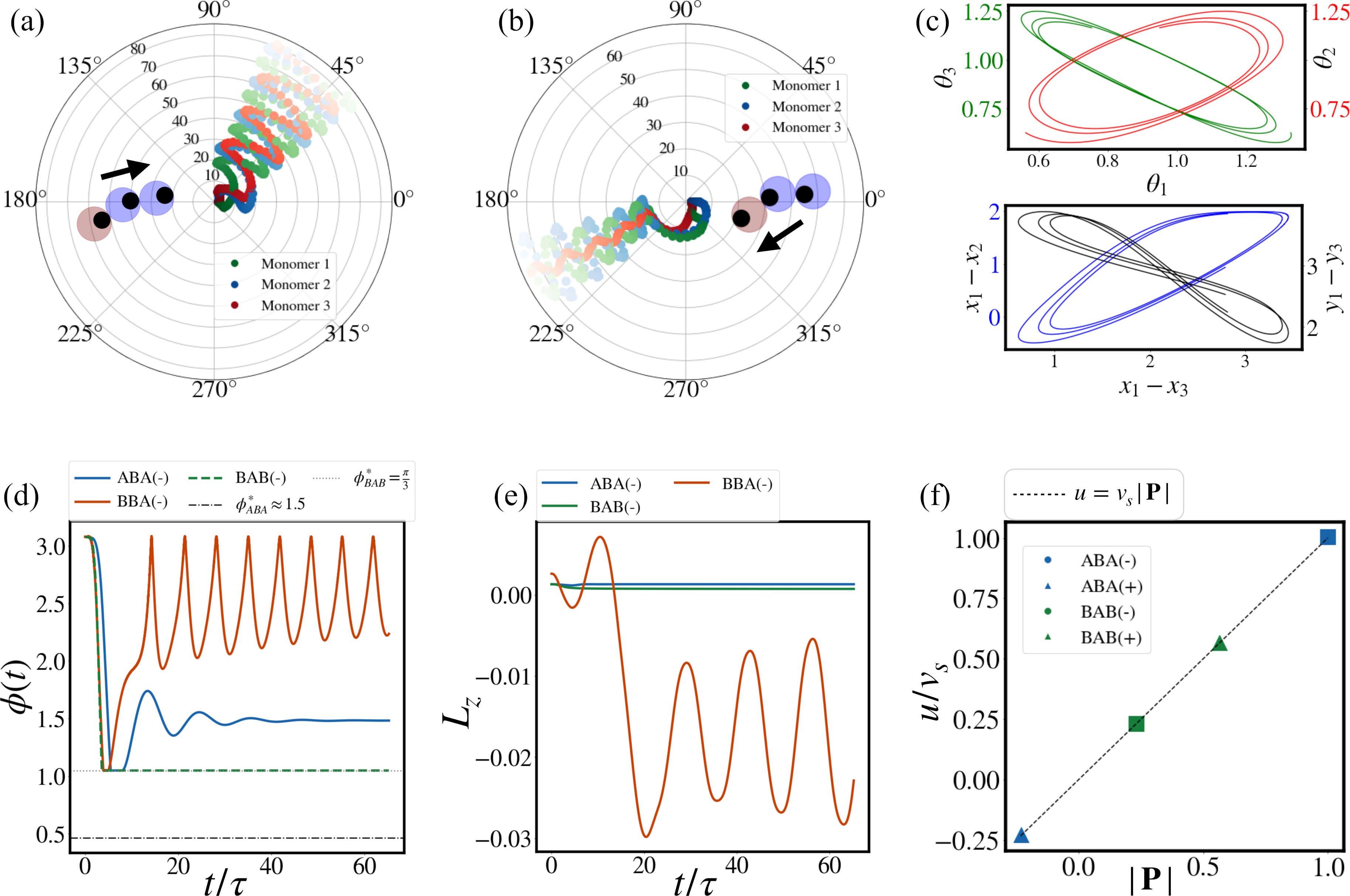
Figure 10: Sustained oscillation in BBA trimer due to anti-symmetric chemical affinities. Panel (a) and (b) display polar plots for the dynamics of BBA(-) and BBA(+) trimers respectively. Panel (c) displays the underlying attractor with the coupling of head and middle orientations to the tail (top) and (hence) a coupling in the reduced coordinate space of $(x_{1}-x_{2},x_{1}-x_{3})$ and $(y_{1}-y_{2},x_{1}-x_{3})$. Note that shared y-axes are used here, the respective quantities are colored same in the plot as in their axis labels. Panel (d) displays both $\phi(t)$, quantifying bond angle dynamics of configurations. Vertical dotted lines indicate steady-state $\phi$ attained by respective configurations. Panel (e) $L_{z}$, capturing the undulation of BBA versus the other two. In (f) validation of (14) is shown for ABA(-),BAB(-),ABA(+), and BAB(+) configurations (excluding the swimmers).

V.3 Trimers: oscillations, swimming, and reversal of motion due to lack of action-reaction symmetry

Having established that dimers perform deterministic chase, we now study the trimer chains, specifically the configurations of ABA, BAB, and BBA. We will use the notation (-)/(+) at the suffix of the configuration to denote whether the configurations have an attractive/repulsive AB interaction. We uncover striking consequences as a result of this additional degree(s) of freedom of the trimer. In particular, chasing as in the previous section is now extended to an undulatory gait (a swimming motion) for BBA(-) and AAB(+), and in addition we will obtain coupled oscillations of ”tail” monomers for ABA(-). Finally, we will see that BAB(-) reverses its direction of motion.

For these configurations, the matrix entries for $\Upsilon_{ij}$ are given by:

$$\Upsilon_{ij}^{ABA}= -\delta_{i1}\delta_{j2}(1-\delta_{i1}\delta_{j2})+\delta_{i2}\delta_{j3}(1-\delta_{i2}\delta_{j3})$$ (25a)

$$+\delta_{i1}\delta_{j3}+\delta_{i3}\delta_{j1}.$$

$$\Upsilon_{ij}^{BAB}= -\Upsilon_{ij}^{ABA}.$$ (25b)

$$\Upsilon_{ij}^{BBA}= -\delta_{i2}\delta_{j1}-\delta_{i1}\delta_{j2}+\delta_{i1}\delta_{j3}(1-\delta_{i1}\delta_{j3})$$

$$+\delta_{i2}\delta_{j3}(1-\delta_{i2}\delta_{j3}).$$ (25c)

We further quantify the dynamics by the bond angle $\phi$ of the trimer. This uniquely specifies the relative monomer positions for the ABA and BAB configurations. We define further an ”angular momentum” of the system

$$L_{z}=\frac{1}{N}\sum_{i}^{N}(\mathbf{V}_{i}\times\mathbf{R})\cdot\mathbf{\hat{z}}$$ (26)

which quantifies net rotations of the monomer about the center of mass (for a 2D system there is only one such component projecting out of plane of the page).

The results are displayed Fig. (9) and Fig. (10). The dynamics of ABA(-) trimer is shown in Fig. (9a). The ABA(-) trimer displays oscillatory angular dynamics since the edge A monomers are repelled from the center and are equally repelled from each other. They eventually stabilize at an angle of $\phi\approx 105.9^{\circ}$, as shown in Fig. (10c) (blue curve). For ABA and BAB where the interactions are symmetric, $\phi$ can be shown to uniquely specify the dynamics, and that the effective system lies in $\{\phi,\theta_{1}\}$. We get (see Appendix(D)):

$$\dot{\phi}=\frac{v_{s}}{2b}\sin\Big{(}\theta_{1}\Big{)}\sec(\frac{\phi}{2})\quad 0\leq\phi<\pi$$ (27)

Thus, the bond angle stabilizes when $\theta_{1}=0$ as in the ABA case (Fig. (9a)).

Similar to the procedure outlined in the previous section, the dynamics of the $ABA(-)$ can be reduced $\{x_{1},x_{2},y_{1},y_{2},e_{x_{1}},e_{x_{2}},e_{y_{1}},e_{y_{2}}\}\rightarrow\{R_{x}\}$ at the fixed point (see Appendix (D)),

$$\frac{dR_{x}}{dt}=v_{s}\Big{(}2\cos(\theta_{1}^{*})+\cos(\theta_{2}^{*})\Big{)}=3v_{s}$$ (28)

thus the stable propelling trimer is analogous to Eq. (24) with a proportional propulsion speed.

The dynamics of BAB(-) configuration in shown in Fig. (9b) (see SI video [29]). We see that the trimer reverses its direction. The cardiod-resembling polar trajectory plateaus at $|R(t)|\approx 14b$, after which the trimer reverse in direction, eventually reaching the origin. The mechanism for this is clear - the edge B monomers are repelled from the central A but are mutually attracted to one another. The equation governing the fixed point propulsion analogous to Eq. (28) is

$$\frac{dR_{x}}{dt}=v_{s}\Big{(}1+2\cos(\theta_{1}^{*})\Big{)}$$ (29)

Noting that $\theta_{1}^{*}\approx\pi$ (Fig 9), we see that the center of mass propels in the -ve $x$ direction. Note that this ”reversal time scale” can be tuned by setting $\frac{\tau_{f}}{\tau}$ accordingly (for large $\frac{\tau_{f}}{\tau}$ the system will reverse quicker). The steady state $\phi$ of the trimer is straightforwardly given by $\frac{\pi}{3}$ (close packed), which we see in Fig. (9).

Finally, we have the result for the BBA(-) configuration in Fig. (10a) (see SI Movie [29]). We see an emergent undulatory gait motion, reminiscent of a micro-swimmer [49]. The behaviour is driven by a competition for alignment between the tailing A and the central B monomer with the leading B monomer. After an initial transient, the system settles into an oscillatory state indefinitely within the time scale of the simulation. This oscillatory behaviour is characterised by limit cycles in phase space, as is shown in Fig. (10b). On the top panel, we see that both $\theta_{3}$ and $\theta_{1}$ are independently coupled to $\theta_{1}$. On the bottom panel, we see that, as a consequence, the relative coordinates $\mathbf{x}_{1}-\mathbf{x}_{2}$ and $\mathbf{x}_{1}-\mathbf{x}_{3}$ are coupled. The oscillations are captured by $\phi$ and $L_{z}$ (26) - see Fig. (10c). In particular, $L_{z}$ differentiates BBA(-)s’ dynamics with the other configurations, as undulations give rise to time-periodic oscillations in both bond angle and an angular momentum w.r.t center-of-mass. Such temporal periodic waves have also been reported in other non-reciprocal models of active matter [42, 43, 44, 46], with the key difference being that in these the activity arises purely due to the non-reciprocity, with the systems otherwise being in equilibrium. Our travelling states here are thus driven by both the polar nature of the chain and the underlying anti-symmetric chemical interactions.

We note that there are three other configurations for the trimer case. The results for these three cases: ABA(+), BAB(+), and BBA(+) are shown in Appendix (E). Finally, we also have a validity of our scaling relation (14) for the ABA and BAB configurations, owing to their symmetric histories of the trajectories (see Appendix (D)). This is displayed in Fig. (10 d).

VI Summary and discussions

In summary we have studied the dynamics of chemically self-interacting active colloidal chains under a wide range of possible interactions, where we have uncovered a breadth of novel phenomenon, namely (i) emergent rigidity and symmetries when the interactions are chemo-repulsive, (ii) crystallization for the chemo-attractive interactions, and (iii) oscillations and direction reversal in non-reciprocally self-interacting chains.

Given that the $3N$ equations of motion with history dependence in Eqs. (1-2) are analytically intractable, the general theoretical approach employed in this work is that of effective descriptions of the dynamics given by either (i) relevant length and time scales of the system (and hence dimensionless parameters), and (ii) time-averaged relationships between order parameters of the system. Not all the time(length) scales are to be analyzed on the same footing though, for instance studying the relative effect of $\tau_{f}$ ($l_{r}$) vs $\tau$ ($b$) is a meaningless comparison without having $\tau_{c}<\tau$ ($l_{d}>b$), as it is a prerequisite for any deterministic spatial structures to form in the system, given the history dependence in Eq. (5). For the dimer cases, this dimensionality reduction procedure enables a reduction from a 6 to 3 dimensional phase space description. This can only be done by exploiting the symmetries of the dynamics, given the aforementioned history dependence of the dynamics. The dimensionality reduction approach here employs the symmetries as seen from simulations, thus coarse grained quantities (e.g. (14)) or equations of motion (e.g. Eq. (28)) emerge from exploiting a symmetry a posteriori of performing a simulation. This is in contrast to other dimensionality reduction methods applied in dynamical systems, such as dynamical principal components analysis [50], which exploit some inherent a priori structure of the state-space.

For the chemo-attractive case, the “chain crystallization” reported here is distinct from other non-equilibrium colloidal crystallization mechanisms [36, 1, 34, 35, 8, 46] in a few ways. Firstly, crystallization and dissipation of the initial state occurs due to long-ranged chemical attraction that depends on the history, and indeed we have observed that such a mechanism does not happen when the history is turned off in Eq. (5). Moreover, this crystallization may be viewed as a “stereotyped folding” of the chain due to the restricted configuration space of the final hexagonal packed crystal. Throughout the dynamics of the collapse, we have observed that the chain transitions from a positionally and configurationally symmetric state to another symmetry configuration (characterizing the final crystal), with pronounced re-arrangements of positions, orientations and configurations in between (see SI Video [29]). This distinguishes it from equilibrium colloidal crystallization [51] and non-equilibrium mechanisms [1, 34, 35, 8], whose packing configuration space is effectively infinite, and no such symmetries are obviously applicable. Possible further study in this direction could be to study the symmetries of the final packed configuration as a function of chain length, interaction parameters and species types [10].

For the trimer cases, we have uncovered colloidal molecules that display sustained oscillations and change in motion direction. The former is distinguished from other works reporting sustained travelling states [48, 25, 42, 43] in that our sustained oscillations arise due to anti-symmetric chemical interactions in addition to an already polar (out-of-equilibrium) chain, and indeed bear resemblance to experimental swimmers found in systems with other propulsion mechanisms [52, 13]. To construct swimmers beyond trimer molecules, we require an additional species C with spatially local chemical affinities with each other and globally attractive towards species B (shown in the SI [29]). The direction reversal on the other hand is distinct from various mechanisms mentioned in the literature [13, 16] which require external inputs to change the propulsion direction; here we have reported on a mechanism that is purely self-generated, by exploiting the non-reciprocal nature of the chemical interactions between the species in the chain. Constructing more elaborate molecules (beyond trimers) that exhibit such a dynamical feature could be possible future work.

Potential generalizations of this work include extending the study to 3D. Such binary colloidal chain studied here can also be used to design initial states with specific steady-state structure and/or dynamics; for example, an $A_{3}B_{7}A_{3}$ configuration gives a stably propelling nucleus of B type surrounded by A type “shields” (see SI Movie [29]), whilst the $B_{7}A_{5}$ chain gives a stably rotating lattice (chirality) - a stationary nucleus of Type B being propelled by a rim of Type A (see SI Movie [29]). Extending this work to multiple species chains, we envisage that these active dynamical features can also potentially be programmed [10] by merely tuning the interactions between species or the initial chain configuration.

In terms of connection to experiments, we note that at a modelling level, we note that we have ignored hydrodynamic interactions. This is rationalised by the fact hydrodynamic fields decay more quickly than chemical fields in strong 2D confinement in Hele-Shaw cells, and thus do not affect our results significantly [22]. Experimental design of chasing interactions in colloids have been realized (e.g. [41]), and our results thus provide testable predictions for phenomenon described here.

Appendix A Simulation details

The model described in Section II has been numerically simulated in an unbounded two-dimensional (2D) space using a custom Cython code (Python on top of a C backend). Throughout the paper, we have used: $b=25\mu m$, $v_{s}=50\mu m/s$, $k_{sp}=1.74\times 10^{4}\mu m/s^{2}$, and $\chi_{r}=7.5\times 10^{3}\mu m^{3}/s^{2}$. For the chemo-repulsive case (Figures 2, 3), $dt=0.01$. For the chemo-attractive and binary species cases (Figures 5, 6, 7, 8, 9, 10, 12) $dt=0.0018$. Unless varied (as in Figures 3, 6) $D_{c}=2500\mu m^{2}/s$, $\mathcal{A}_{1}=10^{-2}$, $\mathcal{A}_{2}=0$ (with $D_{r}=0$).

Appendix B Derivation of orientational fixed point symmetry

We derive here the condition for the orientational fixed points for a representative $N=5$ case, given by (17). This is shown in Fig. (3).

From (2), note that the orientational fixed points are reached if $\mathbf{e}_{i}^{*}\propto\mathbf{J}_{i}$. Let us define

$$\Delta x_{ij}(t,t^{\prime}) =x_{i}(t)-x_{j}(t^{\prime})\quad$$ (30)

$$\mathcal{F}_{ij}^{(x)}(t,t^{\prime}) =\exp\left[-\frac{[x_{i}(t)-x_{j}(t^{\prime})]^{2}}{\mathcal{D}(t,t^{\prime})}\right]$$ (31)

and likewise for $\Delta y_{ij}(t,t^{\prime})$, $\mathcal{F}_{ij}(t,t^{\prime})^{(y)}$ by the substitution $x\rightarrow y$. Then, $e^{*}_{x}$ are (from (5))

$$e_{x_{1}}^{*}\propto\int dt^{\prime}\Bigg{[}\frac{\Delta x_{12}(t,t^{\prime})}{\mathcal{D}(t,t^{\prime})}\mathcal{F}^{(x)}_{12}(t,t^{\prime})+\frac{\Delta x_{13}(t,t^{\prime})}{\mathcal{D}(t,t^{\prime})}\mathcal{F}^{(x)}_{13}(t,t^{\prime})$$ (32)

$$+\frac{\Delta x_{14}(t,t^{\prime})}{\mathcal{D}(t,t^{\prime})}\mathcal{F}^{(x)}_{14}(t,t^{\prime})\Big{]}+\frac{\Delta x_{15}(t,t^{\prime})}{\mathcal{D}(t,t^{\prime})}\mathcal{F}^{(x)}_{15}(t,t^{\prime})\Big{]}$$

$$e_{x_{2}}^{*}\propto\int dt^{\prime}\Bigg{[}\frac{\Delta x_{21}(t,t^{\prime})}{\mathcal{D}^{2}(t,t^{\prime})}\mathcal{F}^{(x)}_{21}(t,t^{\prime})+\frac{\Delta x_{23}(t,t^{\prime})}{\mathcal{D}^{2}(t,t^{\prime})}\mathcal{F}^{(x)}_{23}(t,t^{\prime})$$

$$+\frac{\Delta x_{24}(t,t^{\prime})}{\mathcal{D}^{2}(t,t^{\prime})}\mathcal{F}^{(x)}_{24}(t,t^{\prime})\Big{]}+\frac{\Delta x_{25}(t,t^{\prime})}{\mathcal{D}^{2}(t,t^{\prime})}\mathcal{F}^{(x)}_{25}(t,t^{\prime})\Big{]}$$

$$e_{x_{3}}^{*}\propto\int dt^{\prime}\Bigg{[}\frac{\Delta x_{31}(t,t^{\prime})}{\mathcal{D}^{2}(t,t^{\prime})}\mathcal{F}^{(x)}_{31}(t,t^{\prime})+\frac{\Delta x_{32}(t,t^{\prime})}{\mathcal{D}^{2}(t,t^{\prime})}\mathcal{F}^{(x)}_{32}(t,t^{\prime})$$

$$+\frac{\Delta x_{34}(t,t^{\prime})}{\mathcal{D}^{2}(t,t^{\prime})}\mathcal{F}^{(x)}_{34}(t,t^{\prime})\Big{]}+\frac{\Delta x_{35}(t,t^{\prime})}{\mathcal{D}^{2}(t,t^{\prime})}\mathcal{F}^{(x)}_{35}(t,t^{\prime})\Big{]}$$

$$e_{x_{4}}^{*}\propto\int dt^{\prime}\Bigg{[}\frac{\Delta x_{41}(t,t^{\prime})}{\mathcal{D}^{2}(t,t^{\prime})}\mathcal{F}^{(x)}_{41}(t,t^{\prime})+\frac{\Delta x_{42}(t,t^{\prime})}{\mathcal{D}^{2}(t,t^{\prime})}\mathcal{F}^{(x)}_{42}(t,t^{\prime})$$

$$+\frac{\Delta x_{43}(t,t^{\prime})}{\mathcal{D}^{2}(t,t^{\prime})}\mathcal{F}^{(x)}_{43}(t,t^{\prime})\Big{]}+\frac{\Delta x_{45}(t,t^{\prime})}{\mathcal{D}^{2}(t,t^{\prime})}\mathcal{F}^{(x)}_{45}(t,t^{\prime})\Big{]}$$

$$e_{x_{5}}^{*}\propto\int dt^{\prime}\Bigg{[}\frac{\Delta x_{51}(t,t^{\prime})}{\mathcal{D}^{2}(t,t^{\prime})}\mathcal{F}^{(x)}_{51}(t,t^{\prime})+\frac{\Delta x_{52}(t,t^{\prime})}{\mathcal{D}^{2}(t,t^{\prime})}\mathcal{F}^{(x)}_{52}(t,t^{\prime})$$

$$+\frac{\Delta x_{53}(t,t^{\prime})}{\mathcal{D}^{2}(t,t^{\prime})}\mathcal{F}^{(x)}_{53}(t,t^{\prime})\Big{]}+\frac{\Delta x_{54}(t,t^{\prime})}{\mathcal{D}^{2}(t,t^{\prime})}\mathcal{F}^{(x)}_{54}(t,t^{\prime})\Big{]}$$

The symmetries given by (16) renders

$$\Delta x_{1i}=\Delta x_{5i}\quad\Delta x_{2i}=\Delta x_{4i},\quad\forall i$$ (33)

we thus see straightforwardly that $e_{x_{1}}^{*}=e_{x_{5}}^{*}$ since $\Delta x_{12}=\Delta x_{52}$, $\Delta x_{13}=\Delta x_{53}$, $\Delta x_{14}=\Delta x_{54}$, and $\Delta x_{11}=\Delta x_{55}$. Now using $\Delta x_{22}=\Delta x_{44}$, $\Delta x_{23}=\Delta x_{43}$, $\Delta x_{24}=\Delta x_{24}$, and $\Delta x_{21}=\Delta x_{41}$, we have $e_{x_{2}}^{*}=e_{x_{4}}^{*}$. Since this is an odd-numbered chain $e_{x_{3}}$ takes a standalone value. We can show this to be $1$ by finding $e_{y_{3}}^{*}$, instead of explicitly evaluating the integrals. This proves the $x$ component of (17). For the $y$ component, we can repeat the procedure with $x\rightarrow y$ substitution in (32). Using (15), we get

$$\Delta y_{12}=\Delta y_{54},\quad\Delta y_{13}=\Delta y_{53}$$ (34)

$$\Delta y_{14}=-\Delta y_{52},\quad\Delta y_{14}=-\Delta y_{51}$$ (35)

$$\Delta y_{21}=-\Delta y_{45},\quad\Delta y_{23}=-\Delta y_{43}\quad$$ (36)

$$\Delta y_{24}=-\Delta y_{42},\quad\Delta y_{25}=-\Delta y_{41}$$ (37)

which implies that $e_{y_{1}}=-e_{y_{5}}$, $e_{y_{2}}=-e_{y_{4}}$ from (32). To prove that $e_{y_{3}}=0$, we use

$$\Delta y_{31}=-\Delta y_{53}\quad\Delta y_{23}=-\Delta y_{32}$$ (38)

which completes the proof of (17). ($e_{y_{3}}=0\implies e_{x_{3}}=1$) For an arbitrary $N$, these results generalize straightforwardly to (18). For odd numbered chains, the middle monomer always has $e_{x}=1,\quad e_{y}=0$.

Appendix C Derivation of dimensionality reduction for mondisperse dimers

To reduce the dimensionality of the dimer chain, using (18), we have that

$$\frac{dR_{x}}{dt} =v_{s}\Big{(}\cos(\theta_{1})+\cos(\theta_{2})\Big{)}$$ (39)

$$\frac{dR_{y}}{dt} =v_{s}\Big{(}\sin(\theta_{1})+\sin(\theta_{2})\Big{)}=0$$ (40)

$$\frac{d\theta_{1}}{dt} =\chi_{r}(e_{x_{1}}\mathcal{I}_{b}-e_{y_{1}}\mathcal{I}_{11}^{(x)})$$ (41)

$$\frac{d\theta_{2}}{dt} =\chi_{r}(e_{x_{2}}\mathcal{I}_{b}-e_{y_{2}}\mathcal{I}_{22}^{(R_{x})})=(e_{x_{2}}\mathcal{I}_{b}-e_{y_{2}}\mathcal{I}_{11}^{(R_{x})})$$ (42)

where we have defined

$$\mathcal{I}_{b} =\int_{0}^{t-1}\frac{2b}{(4D_{c}(t-t^{\prime}))^{2}}\exp\Big{(}\frac{-4b^{2}}{\mathcal{D}(t,t^{\prime})}\Big{)}dt^{\prime}$$ (43)

$$\mathcal{I}_{11}^{(x)} =\frac{1}{2}\int_{0}^{t-1}\frac{\Delta R_{x}(t,t^{\prime})}{(4D_{c}(t-t^{\prime}))^{2}}\exp\Big{(}\frac{-\Delta R_{x}^{2}}{\mathcal{D}(t,t^{\prime})}\Big{)}dt^{\prime}=\mathcal{I}_{22}^{(x)}$$

where in the latter, we have used $x_{1}=\frac{1}{2}R_{x}$ by the symmetry, and $\Delta x_{11}(t,t^{\prime})=\Delta x_{22}(t,t^{\prime})$. To evaluate the integrals (C), we use the fact that $\frac{b}{l_{d}}<<1$, which applies in Phase IV, to expand the integrand $\exp\Big{[}-\frac{(R_{x}(t)-R_{x}(t^{\prime}))^{2}}{4D_{c}(t-t^{\prime})}\Big{]}\approx 1-O(\frac{b}{l_{d}}^{2})$. Thus

$$\mathcal{I}_{b} =\int_{0}^{t-1}dt^{{}^{\prime}}\frac{2b}{(4D_{c}(t-t^{\prime}))^{2}}\Big{[}1+O(\frac{b}{l_{d}}^{2})\Big{]}\approx\frac{b}{16D_{c}^{2}}$$ (44)

$$\mathcal{I}_{11}\approx\frac{1}{2}\dot{R}_{x}\int_{0}^{t-1}dt^{{}^{\prime}}\frac{1}{(4D_{c})^{2}(t-t^{\prime})}\Big{[}1+O(\frac{b}{l_{d}}^{2})\Big{]}$$ (46)

$$\approx\frac{\dot{R}_{x}}{32D_{c}^{2}}\int_{0}^{t-1}\frac{1}{(t-t^{\prime})}=\frac{\dot{R}_{x}}{32D_{c}^{2}}\ln(t)$$

thus we have an explicit $t$ dependence on the dynamics of (C), a signature of history build-up of the chemicals due to (5).

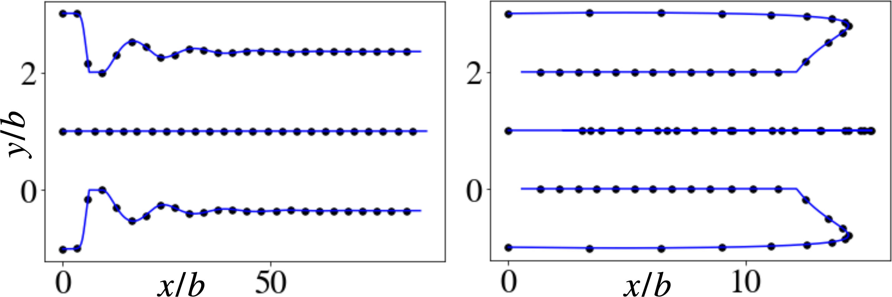
Figure 11: Symmetric trails of ABA(-), BAB(-).

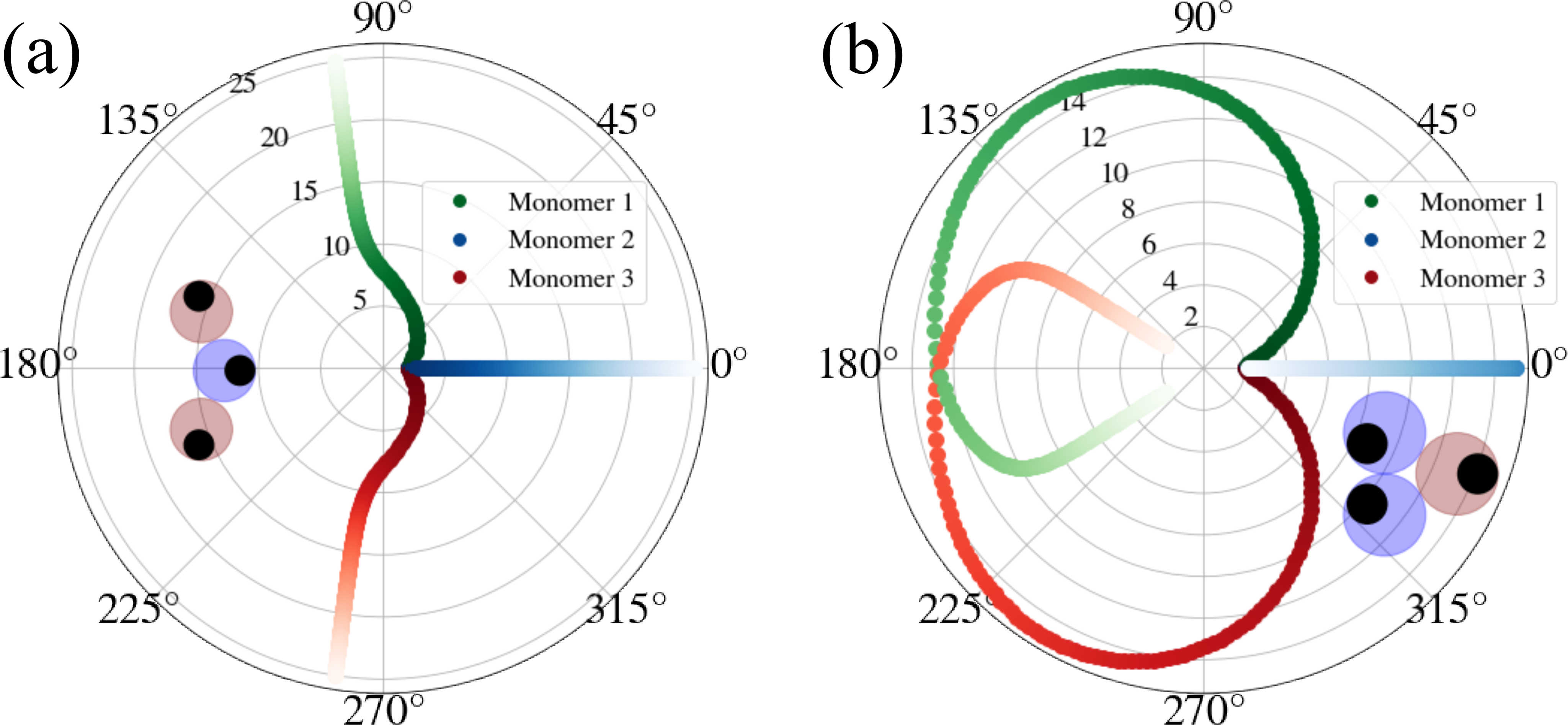
Figure 12: Plots analogous to Figures 9 are displayed, this time for ABA(+), BAB(+) configurations.

Appendix D Symmetric trimers - ABA, BAB

For the ABA and BAB configurations, to solve for $\phi$, we note that the cosine rule implies

$$(\Delta y_{13})^{2}=8b^{2}\Big{(}1-\cos(\phi)\Big{)}$$ (47)

the symmetry of the trimer problem means that the spring forces $F_{12}=-F_{21}$, $F_{23}=-F_{32}$, and further $|F_{12}|=|F_{32}|$. We thus have that

$$\frac{d(\Delta y_{13})}{dt}=2v_{s}\sin(\theta_{1})$$ (48)

Differentiating (47), and applying (37) we arrive at (27).

The symmetry of the trails (see Fig. (11)), further enables us to reduce the effective dimensionality. We consider the $\theta_{1}$ equations for the ABA system:

$$\frac{d\theta}{dt}=\chi_{r}\Big{(}\cos(\theta_{1}){J}_{y_{1}}-\sin(\theta_{1}){J}_{x_{1}}\Big{)}$$ (49)

with

$${J}_{y_{1}}=\int dt^{{}^{\prime}}\Big{[}-\frac{\Delta y_{12}(t,t^{\prime})}{\mathcal{D}^{2}(t,t^{\prime})}\mathcal{F}^{(y)}_{12}+\frac{\Delta y_{13}(t,t^{\prime})}{\mathcal{D}^{2}(t,t^{\prime})}\mathcal{F}^{(y)}_{13}\Big{]}$$ (50)

where we have inserted entries from (25). We can show that ${J}_{y_{1}}=-{J}_{y_{3}}$ by noting the following relations (analogous to (37))

$$\Delta y_{12}=-\Delta y_{32},\quad\Delta y_{13}=-\Delta y_{31}$$ (51)

along with ${J}_{x_{1}}={J}_{x_{3}}$ implies that

$$\frac{d\theta_{1}}{dt}=-\frac{d\theta_{3}}{dt}$$ (52)

as is also evident in Fig. (9) and SI Movie [29]. Thus, at the fixed point orientations $\theta_{i}^{*}$, we have a stably propelling trimer governed by

$$\frac{dR_{x}}{dt}=v_{s}\Big{(}2\cos(\theta_{1})+\cos(\theta_{2})\Big{)}$$ (53)

thus giving (28) and (29)

Appendix E Trimers with AB(+): Results

The results for ABA(+), BAB(+), are displayed here in Fig. (12). ABA(+) reproduces a chemo-repulsive trimer, BAB(+) reproduces a chemo-attractive trimer.

References

- Cates and Tailleur [2015] M. E. Cates and J. Tailleur, Motility-induced phase separation, Annu. Rev. Condens. Matter Phys. 6, 219 (2015).
- Bechinger et al. [2016] C. Bechinger, R. Di Leonardo, H. Löwen, C. Reichhardt, G. Volpe, and G. Volpe, Active particles in complex and crowded environments, Rev. Mod. Phys. 88, 045006 (2016).
- Goldstein [2015] R. E. Goldstein, Green algae as model organisms for biological fluid dynamics, Ann. Rev. Fluid Mech. 47, 343 (2015).
- Ebbens and Howse [2010] S. J. Ebbens and J. R. Howse, In pursuit of propulsion at the nanoscale, Soft Matter 6, 726 (2010).
- Anderson [1989] J. L. Anderson, Colloid transport by interfacial forces, Annu. Rev. Fluid Mech. 21, 61 (1989).
- Snezhko and Aranson [2011] A. Snezhko and I. S. Aranson, Magnetic manipulation of self-assembled colloidal asters, Nat. Mater. 10, 698 (2011).
- Biswas et al. [2021] B. Biswas, D. Mitra, F. Kp, S. Bhat, A. Chatterji, and G. Kumaraswamy, Rigidity dictates spontaneous helix formation of thermoresponsive colloidal chains in poor solvent, ACS Nano 15, 19702 (2021).
- Thutupalli et al. [2018] S. Thutupalli, D. Geyer, R. Singh, R. Adhikari, and H. A. Stone, Flow-induced phase separation of active particles is controlled by boundary conditions, Proc. Natl. Acad. Sci. 115, 5403 (2018).
- Zeravcic et al. [2014] Z. Zeravcic, V. N. Manoharan, and M. P. Brenner, Size limits of self-assembled colloidal structures made using specific interactions, Proc. Natl. Acad. Sci. 111, 15918 (2014).
- Zeravcic et al. [2017] Z. Zeravcic, V. N. Manoharan, and M. P. Brenner, Colloquium: Toward living matter with colloidal particles, Rev. Mod. Phys. 89, 031001 (2017).
- Vutukuri et al. [2017] H. R. Vutukuri, B. Bet, R. Van Roij, M. Dijkstra, and W. T. Huck, Rational design and dynamics of self-propelled colloidal bead chains: from rotators to flagella, Sci. Rep. 7, 16758 (2017).
- Zhang and Granick [2016] J. Zhang and S. Granick, Natural selection in the colloid world: active chiral spirals, Faraday discussions 191, 35 (2016).
- Nishiguchi et al. [2018] D. Nishiguchi, J. Iwasawa, H.-R. Jiang, and M. Sano, Flagellar dynamics of chains of active janus particles fueled by an AC electric field, New J. Phys. 20, 015002 (2018).
- Yan et al. [2012] J. Yan, M. Bloom, S. C. Bae, E. Luijten, and S. Granick, Linking synchronization to self-assembly using magnetic janus colloids, Nature 491, 578 (2012).
- Yang et al. [2020] T. Yang, B. Sprinkle, Y. Guo, J. Qian, D. Hua, A. Donev, D. W. Marr, and N. Wu, Reconfigurable microbots folded from simple colloidal chains, Proc. Natl. Acad. Sci. 117, 18186 (2020).
- Reyes Garza et al. [2023] R. Reyes Garza, N. Kyriakopoulos, Z. M. Cenev, C. Rigoni, and J. V. Timonen, Magnetic quincke rollers with tunable single-particle dynamics and collective states, Sci. Adv. 9, eadh2522 (2023).
- Sagebiel et al. [2017] S. Sagebiel, L. Stricker, S. Engel, and B. J. Ravoo, Self-assembly of colloidal molecules that respond to light and a magnetic field, Chem. Commun. 53, 9296 (2017).
- McMullen et al. [2018] A. McMullen, M. Holmes-Cerfon, F. Sciortino, A. Y. Grosberg, and J. Brujic, Freely jointed polymers made of droplets, Phys. Rev. Lett. 121, 138002 (2018).
- Doi and Edwards [1988] M. Doi and S. F. Edwards, The theory of polymer dynamics, Vol. 73 (Oxford University Press, 1988).
- Laskar and Adhikari [2015] A. Laskar and R. Adhikari, Brownian microhydrodynamics of active filaments, Soft matter 11, 9073 (2015).
- Winkler and Gompper [2020] R. G. Winkler and G. Gompper, The physics of active polymers and filaments, J. Chem. Phys. 153 (2020).
- Kumar et al. [2023] M. Kumar, A. Murali, A. G. Subramaniam, R. Singh, and S. Thutupalli, Emergent dynamics due to chemo-hydrodynamic self-interactions in active polymers, arXiv preprint arXiv:2303.10742 (2023).
- Herminghaus et al. [2014] S. Herminghaus, C. C. Maass, C. Krüger, S. Thutupalli, L. Goehring, and C. Bahr, Interfacial mechanisms in active emulsions, Soft matter 10, 7008 (2014).
- Hokmabad et al. [2022] B. V. Hokmabad, J. Agudo-Canalejo, S. Saha, R. Golestanian, and C. C. Maass, Chemotactic self-caging in active emulsions, Proc. Natl. Acad. Sci. 119, e2122269119 (2022).
- Saha et al. [2014] S. Saha, R. Golestanian, and S. Ramaswamy, Clusters, asters, and collective oscillations in chemotactic colloids, Phys. Rev. E 89, 062316 (2014).
- Sengupta et al. [2009] A. Sengupta, S. van Teeffelen, and H. Löwen, Dynamics of a microorganism moving by chemotaxis in its own secretion, Phys. Rev. E 80, 031122 (2009).
- Note [1] There is an additional which we ignore.
- Note [2] With the definitions given in equations (6) and (7) there are additional valid (6 in total) Peclet numbers. However, these additional feasible dimensionless parameters in our system e.g. one could define ), are not systematically studied here (indeed they do not affect our bigger picture findings).
- [29] See the supplemental material at this url: .
- Helfrich [1973] W. Helfrich, Elastic properties of lipid bilayers: theory and possible experiments, Z. Naturforsch 28, 693 (1973).
- Tsori and De Gennes [2004] Y. Tsori and P.-G. De Gennes, Self-trapping of a single bacterium in its own chemoattractant, EPL 66, 599 (2004).
- Soto and Golestanian [2014] R. Soto and R. Golestanian, Self-assembly of catalytically active colloidal molecules: Tailoring activity through surface chemistry, Phys. Rev. Lett. 112, 068301 (2014).
- Agudo-Canalejo and Golestanian [2019] J. Agudo-Canalejo and R. Golestanian, Active phase separation in mixtures of chemically interacting particles, Phys. Rev. Lett. 123, 018101 (2019).
- Palacci et al. [2013] J. Palacci, S. Sacanna, A. P. Steinberg, D. J. Pine, and P. M. Chaikin, Living crystals of light-activated colloidal surfers, Science 339, 936 (2013).
- Singh and Adhikari [2016] R. Singh and R. Adhikari, Universal hydrodynamic mechanisms for crystallization in active colloidal suspensions, Phys. Rev. Lett. 117, 228002 (2016).
- Theurkauff et al. [2012] I. Theurkauff, C. Cottin-Bizonne, J. Palacci, C. Ybert, and L. Bocquet, Dynamic clustering in active colloidal suspensions with chemical signaling, Phys. Rev. Lett. 108, 268303 (2012).
- Niu et al. [2018] R. Niu, A. Fischer, T. Palberg, and T. Speck, Dynamics of binary active clusters driven by ion-exchange particles, ACS Nano 12, 10932 (2018).
- Yu et al. [2018] T. Yu, P. Chuphal, S. Thakur, S. Y. Reigh, D. P. Singh, and P. Fischer, Chemical micromotors self-assemble and self-propel by spontaneous symmetry breaking, Chem. Commun. 54, 11933 (2018).
- Schmidt et al. [2019] F. Schmidt, B. Liebchen, H. Löwen, and G. Volpe, Light-controlled assembly of active colloidal molecules, J. Chem. Phys. 150 (2019).
- Grauer et al. [2020] J. Grauer, H. Löwen, A. Be’er, and B. Liebchen, Swarm hunting and cluster ejections in chemically communicating active mixtures, Sci. Rep. 10, 5594 (2020).
- Meredith et al. [2020] C. H. Meredith, P. G. Moerman, J. Groenewold, Y.-J. Chiu, W. K. Kegel, A. van Blaaderen, and L. D. Zarzar, Predator–prey interactions between droplets driven by non-reciprocal oil exchange, Nat. Chem. 12, 1136 (2020).
- Saha et al. [2020] S. Saha, J. Agudo-Canalejo, and R. Golestanian, Scalar active mixtures: The nonreciprocal Cahn-Hilliard model, Phys. Rev. X 10, 041009 (2020).
- You et al. [2020] Z. You, A. Baskaran, and M. C. Marchetti, Nonreciprocity as a generic route to traveling states, Proc. Natl. Acad. Sci. 117, 19767 (2020).
- Scheibner et al. [2020] C. Scheibner, A. Souslov, D. Banerjee, P. Surówka, W. T. Irvine, and V. Vitelli, Odd elasticity, Nat. Phys. 16, 475 (2020).
- Braverman et al. [2021] L. Braverman, C. Scheibner, B. VanSaders, and V. Vitelli, Topological defects in solids with odd elasticity, Phys. Rev. Lett. 127, 268001 (2021).
- Tan et al. [2022] T. H. Tan, A. Mietke, J. Li, Y. Chen, H. Higinbotham, P. J. Foster, S. Gokhale, J. Dunkel, and N. Fakhri, Odd dynamics of living chiral crystals, Nature 607, 287 (2022).
- Tsyganov et al. [2003] M. Tsyganov, J. Brindley, A. Holden, and V. Biktashev, Quasisoliton interaction of pursuit-evasion waves in a predator-prey system, Phys. Rev. Lett. 91, 218102 (2003).
- Sengupta et al. [2011] A. Sengupta, T. Kruppa, and H. Löwen, Chemotactic predator-prey dynamics, Phys. Rev. E 83, 031914 (2011).
- Fang-Yen et al. [2010] C. Fang-Yen, M. Wyart, J. Xie, R. Kawai, T. Kodger, S. Chen, Q. Wen, and A. D. Samuel, Biomechanical analysis of gait adaptation in the nematode Caenorhabditis Elegans, Proc. Natl. Acad. Sci. 107, 20323 (2010).
- Williams et al. [2018] A. H. Williams, T. H. Kim, F. Wang, S. Vyas, S. I. Ryu, K. V. Shenoy, M. Schnitzer, T. G. Kolda, and S. Ganguli, Unsupervised discovery of demixed, low-dimensional neural dynamics across multiple timescales through tensor component analysis, Neuron 98, 1099 (2018).
- Li et al. [2016] B. Li, D. Zhou, and Y. Han, Assembly and phase transitions of colloidal crystals, Nat. Rev. Mater. 1, 1 (2016).
- Dreyfus et al. [2005] R. Dreyfus, J. Baudry, M. L. Roper, M. Fermigier, H. A. Stone, and J. Bibette, Microscopic artificial swimmers, Nature 437, 862 (2005).