Image Synthesis with Graph Conditioning: CLIP-Guided Diffusion Models for Scene Graphs

Abstract

Advancements in generative models have sparked significant interest in generating images while adhering to specific structural guidelines. Scene graph to image generation is one such task of generating images which are consistent with the given scene graph. However, the complexity of visual scenes poses a challenge in accurately aligning objects based on specified relations within the scene graph. Existing methods approach this task by first predicting a scene layout and generating images from these layouts using adversarial training. In this work, we introduce a novel approach to generate images from scene graphs which eliminates the need of predicting intermediate layouts. We leverage pre-trained text-to-image diffusion models and CLIP guidance to translate graph knowledge into images. Towards this, we first pre-train our graph encoder to align graph features with CLIP features of corresponding images using a GAN based training. Further, we fuse the graph features with CLIP embedding of object labels present in the given scene graph to create a graph consistent CLIP guided conditioning signal. In the conditioning input, object embeddings provide coarse structure of the image and graph features provide structural alignment based on relationships among objects. Finally, we fine tune a pre-trained diffusion model with the graph consistent conditioning signal with reconstruction and CLIP alignment loss. Elaborate experiments reveal that our method outperforms existing methods on standard benchmarks of COCO-stuff and Visual Genome dataset.

Figure 1: Samples generated using our architecture. It can be seen that the generated images reflect the structure given in the scene graph. They are different from ground truth images illustrating the diversity in generated samples.

1 Introduction

Scene graph represents a visual scene as a graph where nodes correspond to objects and edges represent relationships or interactions between these objects. Improved generative models now allow users to generate high quality images where they can control the style, structure or layout of the synthesised images. Such conditional image generation allow users to guide the generation using text Rombach et al. (2022a); Ramesh et al. (2021), segmentation mask Park et al. (2019a), class labels Dhariwal and Nichol (2021), scene layout Jahn et al. (2021); Zheng et al. (2023), sketches, stroke paintings Meng et al. (2022), and such more conditional signals. In particular, use of text as a conditioning modality offers a versatile approach, allowing for diverse combinations of inputs, encompassing intricate and abstract concepts. However, leveraging text for conditioning is not without challenges. Natural language sentences tend to be lengthy and loosely structured, relying heavily on syntax for semantic interpretation. The inherent ambiguity in language, where different sentences may convey the same concept, poses a risk of instability during training. This becomes particularly apparent in scenarios where precise description constraints are crucial. In this context, relying solely on text representations for a specific scene may prove to be insufficient.

Motivated by promising results of conditional generation and limitation of text as a conditional signal, in this work we propose a novel method to generate images from scene graphs. First introduced by Johnson et al. (2018), scene graph to image generation is a task of generating images using set of semantic object labels and underlying semantic relationships among these objects. Most of the existing works follow a two stage architecture where they first generate a scene layout and use GAN to synthesize realistic images from these scene layouts Johnson et al. (2018); Ashual and Wolf (2019); Ivgi et al. (2021). Object nodes of scene graph is mapped to bounding boxes in the layout and the relationships are signified by the spatial structure of the layout. While these scene layouts can be effective in representing spatial relationships in the scenes, they fail to capture non-spatial complex relationships among objects. Relationships such as “left of”, “above”, “sorrounding” are spatial relationships, whereas “looking at”, “holding”, “drinking” are examples of non-spatial relationships. Translating scene graphs to accurate layouts and limiting representation capabilities of these layouts results in images inconsistent with the input scene graph.

To overcome the limitations of existing methodologies, we propose to learn an intermediate graph representation while eliminating the need of predicting scene layouts. We use this graph representation as a conditional signal to fine-tune a pre-trained text-to-image diffusion model to generate images conditioned on scene graphs. To harness the strong semantic understanding offered by diffusion models, we propose to predict a conditional graph representation that aligns well with the inherent semantic knowledge of diffusion models. We use CLIP Radford et al. (2021) guidance to generate such graph embeddings.

We first employ a GAN-based CLIP alignment module to train our graph encoder. This module instructs the graph encoder to generate graph embeddings that closely resemble the visual features of corresponding images in the CLIP latent space. To construct an effective conditioning signal for diffusion model, we fuse output of graph encoder with semantic label embedding of objects present in the scene graph. This conditioning signal is prepared to leverage the high prior semantic understanding of text-to-image diffusion models. We use this conditioning signal to fine-tune the diffusion model to generate images conditioned on scene graph. We demonstrate the effectiveness of our method using established benchmarks like Visual GenomeKrishna et al. (2017) and COCO-stuff Caesar et al. (2018). Comparisons with current state-of-the-art methods reveal superior quantitative and qualitative results. We can summarise our contributions as follows:

(1) We propose to learn an effective graph representation, eliminating the need of predicting intermediate layouts to synthesize images. We use this graph representation to construct a suitable conditioning signal for text-to-image diffusion model. This conditioning signal is guided to leverage the semantic knowledge of text-to-image diffusion model.

(2) We propose a training strategy that effectively employs the constructed conditioning signal to fine-tune the diffusion model.

Figure 1 shows the example images generated by our model with the original reference images. Images generated by our model follow the input scene graph. For example, objects and relationships specified in the input scene graph in Figure 1, such as “Birds flying above Boat” and “wall surrounding stop sign” are present in the generated images.

2 Related Works

Diffusion as generative model. The introduction of diffusion models by Sohl-Dickstein et al. (2015) marked a notable approach to image generation. These models operate by learning the reverse process of the forward diffusion, where input is transformed into Gaussian noise. The denosing process is implemented using U-net Oktay et al. (2018) or transformer Vaswani et al. (2017) based models. In order to reduce the computation and training complexity, Rombach et al. (2022b); Vahdat et al. (2021) introduced diffusion models which operate in latent space. Dhariwal and Nichol (2021) proposed conditional generation by diffusion using classifier guidance. Recent advancements in these latent diffusion models have enabled users to produce diverse and realistic high quality images conditioned on various factors such as text Ramesh et al. (2021), artistic style, sketch, pose, and class labels Esser et al. (2023). Diffusion can also be used to generate text Li et al. (2021); Lin et al. (2023), videos Esser et al. (2023); Yu et al. (2023) and graphs Jo et al. (2022). The conditioning is applied using cross attention mechanism between output of individual layers of denoising U-net and given conditional signals. Similar techniques are employed in text-to-image latent diffusion models. Ramesh et al. (2022) uses CLIP latent of text to condition high quality image generation. Saharia et al. (2022) uses latent from large language models such as T5 to condition latent diffusion models. While there has been notable progress in the diffusion-based conditional image synthesis, there exists a notable gap in the exploration of image generation from graph-structured data. In this work we explore the capabilities of text-to-image diffusion models in the task of image generation conditioned on scene graphs.

Image generation from scene graphs. Scene graph represents an image using set of nodes and edges. Nodes represent objects present in the image and their underlying relationships are captured by edges. Conventional scene graph to image methods tackle this task by following two stage architecture. At first a scene layout is predicted from graph. Scene layout represents an image using bounding boxes of corresponding objects present in the image. Scene layout is then translated into an image using convolution neural network based image synthesis models such as SPADE Park et al. (2019b), OC-GAN Sylvain et al. (2021). This task was first introduced by Johnson et al. (2018). They employ a multi layer graph convolution network Kipf and Welling (2016) to get graph representation. This graph representation is used to predict object bounding boxes. The boxes are then used to generate images using cascaded refinement network. Generation is guided by GAN-based setup where a discriminator is employed to generate realistic images. Following Johnson et al. (2018) subsequent works adopt the two stage approach combined with GAN-based generation. Ashual and Wolf (2019) provides a way to control style of generated objects by providing a module to capture the style information of objects. Herzig et al. (2020) use canonicalization for scene graph representation before translating it into scene layouts. This enhances the graph representation by incorporating supplementary information for semantic equivalence. Ivgi et al. (2021) introduces an overlap loss to eliminate object overlapping. Sortino et al. (2023) use transformers for image generation. They learn layout representation using graph transformer. Further an image transformer coupled with VQ-VAE Razavi et al. (2019) is used to sample images from these layouts. Farshad et al. (2023) uses scene layout and segmentation masks at sampling time of diffusion to generate graph aligned images. Zhang et al. (2023) introduce a consistency module to overcome negligence of smaller object in the generated images.

Most of the existing works utilise a layout based representation of graphs and GAN-based image generation. In this work we propose to use a graph representation which aligns well with the semantic prior of diffusion models. We use this aligned graph representation as a conditioning signal for diffusion based image generation. Notably, we eliminate the need for layout generation and convert the two stage to single stage generation.

3 Method

Figure 2: Overview of the proposed architecture. Graph encoder gives CLIP aligned graph embedding. This embedding is fused with semantic label embedding of objects present in the scene graph. The fused embedding forms a conditioning signal for diffusion model. During training, we pass this conditional signal with noise added input image and guide the training using reconstruction and CLIP alignment loss. During sampling we pass this conditioning signal with noise to generate image corresponding to the input scene graph.

In this section, we present our proposed methodology with a detailed description of each component. We first give a brief overview of the conditional diffusion model. Subsequently, we explain the functionality of the graph encoder, and the process of obtaining graph representations. In section 3.3, we explain the creation of a CLIP-guided graph conditioning for diffusion model, along with the training strategy. Finally, we describe our GAN-based CLIP alignment module. An overview of our methodology is given in Figure 2.

3.1 Background for diffusion

Diffusion models form a class of generative models designed to simulate the process of data generation through a series of diffusion steps. They constitute probabilistic generative models trained to comprehend data distributions through the sequential denoising of a variable sampled from a given distribution, mainly Gaussian. In the context of conditional generation, the goal is to generate data conditioned on some input information. For our case, we are concerned with pre-trained text-to-image diffusion model $\hat{x}_{\theta}$. Given noise $\epsilon\sim\mathcal{N}(0,I)$ and conditioning signal $S_{cond}$, the model generates an image $x_{gen}$ as follows:

$${x_{gen}=\hat{x}_{\theta}(\epsilon,S_{cond})}.$$ (1)

U-net based architecture is used to predict the added noise. The training is guided by a squared error loss to denoise an image or latent code with variable levels of noise. It is given by,

$${\mathbb{E}_{(x,\epsilon,t)}\lVert x-\hat{x}_{\theta}(x_{t},S_{cond})\rVert_{2}^{2}},$$ (2)

where $x$ is the reference image, $x_{t}=\alpha_{t}x+\sigma_{t}\epsilon$, is the noisy sample at diffusion time step $t$. $\alpha_{t}$ and $\sigma_{t}$ control the noise schedule. For latent diffusion models, latent embedding of input image is generated using VQGAN Esser et al. (2021) or KL-Autoencoder Rombach et al. (2022b). All diffusion steps are applied in latent space, and then the final latent is decoded into an image.

3.2 Graph Encoder

We use multi layer graph convolution network Kipf and Welling (2016); Johnson et al. (2018) to generate graph features from scene graph. We follow existing architecture of graph encoder for fair comparison with existing methodologies. Scene graph $S$ contains a set of objects $S_{o}$ and a set of relationships $S_{r}$. $S$ is represented using relationship triplets $(o_{i},r_{ij},o_{j})$ where $o_{i}\in S_{o}$ and $o_{j}\in S_{o}$ are two objects from object set $S_{o}$, and $r_{ij}\in S_{r}$ is the relationship between $i^{th}$ and $j^{th}$ object. Graph encoder fuses individual object embedding and individual relationship embedding to give a global scene graph embedding. For object $o_{i}$, we take a set $Out(o_{i})$ to be the set of object to which $o_{i}$ has an outgoing directed edge. Set $In(o_{i})$ denotes the set of objects where $o_{i}$ has an incoming directed edge from these objects. We find embedding for object $o_{i}$ as follows:

$$G_{o_{out}} =F_{o}^{out}(G_{o_{i}},G_{r_{ij}},G_{{o_{j}})_{j\in Out(o_{i})}},$$

$$G_{o_{in}} =F_{o}^{in}(G_{o_{j}},G_{r_{ji}},G_{o_{i}})_{j\in In(o_{i})},$$

$$G_{o_{i}} =F^{pool}((G_{o_{out}})\cup(G_{o_{in}})),$$

where $G_{o_{i}},G_{o_{j}}\in R^{d_{o}}$ are the embeddings of object $o_{i}$ and $o_{j}$ respectively. $G_{r_{ij}},G_{r_{ji}}\in R^{d_{r}}$ are the embeddings for relationship $r_{ij}$ and $r_{ji}$ respectively. $F_{o}^{out},F_{o}^{in}$ are graph convolution layers and $F^{pool}$ is an average pooling layer. Similar to this, we find relationship embedding as follows:

$${G_{r_{ij}}=F^{rel}(G_{o_{i}},G_{r_{ij}},G_{{o_{j}})}},$$ (3)

where $F^{rel}$ is a graph convolution layer. After getting these individual object and relationship embedding, we calculate a global graph feature ${G_{global}^{s}}$ as follows. First we map each object and relationship embedding to same dimension $d_{g}$ using $F^{o}_{d_{g}}$ and $F^{r}_{d_{g}}$. $F^{o}_{d_{g}}$ and $F^{r}_{d_{g}}$ are 2 layer MLP’s. They map $d_{o}$ dimensional object embedding and $d_{r}$ dimension relationship embedding to $d_{g}$ dimensional embedding respectively. After getting same dimension embedding, we find an embedding to represent each individual triplet of scene graph as follows:

$${G_{triplet_{ij}}=F^{o}_{d_{g}}(G_{o_{i}})+F^{r}_{d_{g}}(G_{r_{ij}})+F^{o}_{d_{g}}(G_{o_{j}})}.$$ (4)

Finally, a global embedding $G_{global}^{s}$, for a scene graph $S$ is calculated by concatenating individual triplet embedding and then mapping it to a $d_{g}$ dimensional feature.

$$G_{global}^{s}=F^{global}_{d_{g}}(concat(G_{triplet_{ij}}))_{triplet_{ij}\in S}.$$ (5)

We use $G_{global}^{s}$ while creating a conditioning signal for fine-tuning text-to-image diffusion model.

3.3 Fine-tuning diffusion model with CLIP guided graph conditioning

Let $S_{label}$ denote semantic label of the objects present in scene graph. The semantic labels are passed through CLIP text encoder to generate object label embedding. Then $S$ is passed through a graph encoder to generate embedding $G_{global}^{s}$ using Eq. 5. The object label embedding captures the entity level information of the image, while $G_{global}^{S}$ captures the interaction between these entities. Let $label_{i}$ be the semantic label of $i^{th}$ object present in $S$. Then,

$${S_{label_{i}}=CLIPtext(label_{i})}.$$ (6)

Finally we fuse $G_{global}^{s}$ and $S_{label_{i}}$ for all the labels to generate conditioning signal for fine-tuning the diffusion model.

$${S_{cond}=concat(G_{global}^{s},S_{label_{i}})\;\forall i\in S}.$$ (7)

We add textual padding to generate conditional signals of same dimension irrespective of the number of objects present in the scene graph.

However, we note that the embedding space of $G_{global}^{s}$ and $S_{label_{i}}$ are different. Thus, a simple concatenation is not useful. Further, text-to-image pretrained diffusion models use a specific text encoder such as CLIP’ text encoder. Thus, it is necessary to provide the features that align with the space of CLIP embedding. Otherwise, the domain mismatch may lead to poor image generation. To this end, we guide our graph encoder to generate embeddings aligned with corresponding image features in CLIP space. Next, we discuss the training and alignment strategy.

3.3.1 Training objective

Our learning objective is two-fold. First, diffusion model should learn the underlying distribution of image and scene-graph pairs. Second, we want to map output of graph encoder to a space where it aligns with prior semantic knowledge of text-to-image diffusion models. We achieve these goals in the following manner.

Reconstruction Loss: We use a reconstruction loss to guide the diffusion model to learn the underlying distribution of data. The loss $\mathcal{L}_{recon}$ is given by,

$${\mathcal{L}_{recon}=\mathbb{E}_{(x,S)\sim{\text{data}}}\lVert x-\hat{x}_{\theta}(x_{t},S_{cond})\rVert^{2}_{2}},$$ (8)

where $\hat{x}_{\theta}$ is denoising network of diffusion, $x_{t}$ is the noised sample at diffusion time step $t$, and $S_{cond}$ is the conditioning signal we curated. $(x,S)$ is the image-graph pair, sampled randomly from the data.

Alignment Loss: Towards the second goal of aligning $G_{global}^{s}$ with CLIP space, we apply a mean squared error loss between $G_{global}^{s}$ and CLIP visual features of the corresponding image. For an image-graph pair $(x,S)$, the loss $\mathcal{L}_{CLIP}$ is given by,

$${\mathcal{L}_{CLIP}=\mathbb{E}_{(x,S)\sim{\text{data}}}\lVert G_{global}^{s}-CLIP(x)\rVert_{2}^{2}}.$$ (9)

Additionally, we also use Maximum Mean Discrepancy (MMD) loss Li et al. (2017) to bridge the domain gap between $G_{global}^{s}$ and CLIP visual features. In our experiments we observe that MMD loss makes the training stable, improves quantitative results and quality of images. MMD loss is defined as follows:

$$\mathcal{L}_{MMD}^{2} =\mathbb{E}_{c\sim p({c})}\left[\phi(c,c)\right]$$

$$+\mathbb{E}_{G\sim p(\text{graph})}\left[\phi(G_{global}^{s},G_{global}^{s})\right]$$

$$-2\mathbb{E}_{c\sim p({c}),G\sim p(\text{graph})}\left[\phi(c,G_{global}^{s})\right],$$

where $c$ is the CLIP feature of an input image and $G_{global}^{s}$ is the output of graph encoder for the corresponding scene graph. $\phi$ is the kernel function. We combine both $\mathcal{L}_{CLIP}$ and $\mathcal{L}_{MMD}$ to define an alignment loss as,

$${\mathcal{L}_{align}=\beta\mathcal{L}_{CLIP}+(1-\beta)\mathcal{L}_{MMD}},$$ (10)

where $\beta$ is a hyperparameter.

Total Loss: Now by considering both reconstruction loss and alignment loss we define our training objective as follows:

$${\mathcal{L}_{train}=\lambda\mathcal{L}_{recon}+(1-\lambda)\mathcal{L}_{align}},$$ (11)

where $\lambda$ is a hyperparameter. We fine tune diffusion model and graph encoder using $\mathcal{L}_{train}$.

Though $\mathcal{L}_{align}$ guides the alignment of graph embedding with CLIP feature space, initially the latent space of the graph encoder output differs substantially from the CLIP feature space. To bridge this gap, we propose GAN-based CLIP alignment module (GCA) to pre-train graph encoder. In the following, we discuss GCA.

	COCO-Stuff				Visual Genome
Methods (Reference)	FID$\downarrow$	IS$\uparrow$	DS$\uparrow$	OOR$\uparrow$	FID$\downarrow$	IS$\uparrow$	DS$\uparrow$	OOR$\uparrow$
SG2IM (CVPR’18) ∗	125.58	7.8	0.02	–	92.8	6.5	0.1	–
PasteGAN (NeurIPS’19)∗	70.2	11.28	0.60	–	130	6.5	0.38	–
Specifying (ICCV’19)∗	68.27	15.2	0.67	70.84	–	–	–	–
Canonical (ECCV’20)∗	64.65	14.5	0.70	73.77	45.7	16.4	0.68	72.83
RetrieveGAN (ECCV’20)	56.9	10.2	0.47	–	113.1	7.5	0.30	–
SCSM (AAAI’22)	51.6	15.2	0.63	–	63.7	10.8	0.59	–
SGTransformer (CVIU’23)∗	52.8	15.8	0.57	–	50.16	14.6	0.59	–
SceneGenie (ICCV’23)	63.27	22.16	–	–	42.21	20.25	–	–
LOCI (IJCAI’23)	49.8	15.7	0.65	81.26	44.9	14.6	0.62	79.04
Ours	38.12	30.18	0.73	82.38	35.8	26.2	0.71	81.04

Table 1: Quantitative results on Visual Genome and COCO-Stuff dataset. All the results are either reproduced (^∗) or taken directly from the original papers. Best results are shown in bold letters, and second best results are underlined. Results are reported for $256\times 256$ images.

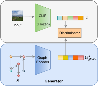
Figure 3: Graph embedding is aligned with CLIP visual features of the corresponding image. Alignment is achieved using GAN-based architecture.

3.4 GAN-based CLIP Alignment

We use GAN-based pre-training to align $G_{global}^{s}$ with CLIP features. Figure 3 provides an overview of our GAN-based CLIP alignment module. We consider graph encoder as our generator and $G_{global}^{s}$ as our generated data. CLIP visual features, $c$, form real data. Discriminator is trained to predict whether the input is from real or generated data. It guides the output of our generator to align with CLIP features. Training of graph encoder is guided by $\mathcal{L}_{\text{graph}}$, where $\mathcal{G}(S)$ is graph encoder output when given a scene graph $S$ as an input. $\mathcal{L}_{\text{graph}}$ is a standard generator loss for GAN-based architectures.

$${\mathcal{L}_{\text{graph}}=\mathbb{E}_{S\sim p(S)}\left[-\log\mathcal{D}(\mathcal{G}(S))\right]}.$$ (12)

Training of discriminator is guided by $\mathcal{L}_{\text{disc}}$, a standard discriminator loss for GAN-based architectures. Let $\mathcal{D}(c)$ be the predicted probability by discriminator when the input is from real distribution (CLIP features, $c$).

$${\mathcal{L}_{\text{disc}}=-\mathbb{E}_{c\sim p(c)}\left[\log\mathcal{D}(c)\right]-\mathbb{E}_{S\sim p(S)}\left[\log(1-\mathcal{D}(\mathcal{G}(S)))\right]}.$$

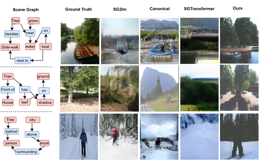
Figure 4: Qualitative comparison of $(256\times 256)$ images generated by various publicly available scene graph to image models. All given input graphs corresponding to ground truth images are perturbed slightly to check effectiveness of each methods. The last columns shows images generated by our method.

3.5 Sampling process

In Figure 3, stage 2 gives an overview for the sampling process. Once the diffusion network is trained, we can sample images from a latent noise $\epsilon$. For a fine-tuned denoising U-net $\hat{x}_{\theta}$, we can sample latent conditioned on scene graph $S$ as follows:

$${x_{latent}=\hat{x}_{\theta}(\epsilon,S_{cond})},$$ (13)

where $S_{cond}$ is the curated graph conditioning signal and $\epsilon\sim\mathcal{N}(0,I)$. $x_{latent}$ is then decoded using diffusion’s latent decoder to get an image. The generated image aligns well with the input scene graph.

4 Experiments

In this section, we outline the implementation details of our approach. We compare our results with existing state-of-the-art scene graph to image models. We verify effectiveness of each component of our training scheme by providing ablation results.

4.1 Experimental setup

4.1.1 Dataset and Evaluation

We train and evaluate our model on COCO-stuff and Visual genome dataset. We follow existing works Johnson et al. (2018); Herzig et al. (2020) to filter out and divide the data into training and validation set for fair comparison. After pre-processing, we get 62,565 image-graph pair in training set and 5,506 image-graph pair in validation set of Visual Genome dataset. COCO-stuff has 40,000 and 5,000 image-graph pairs in training and validation sets respectively. We follow Johnson et al. (2018) to create synthetic scene graphs for COCO-stuff using spatial relationship edges. To show effectiveness of our approach we evaluate our model using Inception Score (IS) Salimans et al. (2016), Fréchet Inception Distance (FID) Heusel et al. (2017), Diversity Score (DS) Zhang (2018), and Object occurrence ratio (OOR) Zhang et al. (2023). IS is a metric commonly used to evaluate the quality and diversity of generated images in generative models. A higher Inception Score indicates better-performing generative models that produce both realistic and diverse images. DS is a measure used to quantify the variety and distinctiveness of generated samples for same input scene graph. FID evaluates the similarity between the distribution of real data and generated data using feature representations extracted from a pre-trained Inception model. OOR is the ratio of the objects detected in the generated image by YOLOv7 Wang et al. (2023) with respect to the objects given in the input scene graph. High OOR implies high consistency of generated images with scene graphs.

4.1.2 Implementation Details

We use a pre-trained stable diffusion model Rombach et al. (2022b). Graph encoder is a standard multi layer graph convolution network taking nodes and edges as input. $d_{g}$ for graph encoder is 512, we take $\lambda=0.7$ and $\beta=0.5$. For reconstruction loss in diffusion, we guide are training with the MSE loss between predicted and added noise. We use Adam optimizer Zhang (2018) with a learning rate of 1e-6. We fine-tune the Diffusion model for 62,000 iteration and 32,525 iterations for Visual Genome and COCO-stuff datasets respectively,with batch size of 2. Discriminator is a 5 layer MLP, trained for 40 epochs with Adam optimizer.

4.2 Results

4.2.1 Quantitative results

Following previous works Zhang et al. (2023); Johnson et al. (2018); Herzig et al. (2020), we have reported a comparison between our method and existing methods using FID score, IS, DS, OOR. Table 1 shows the effectiveness of our method based on these evaluation metric.

On COCO-stuff benchmark, we are able to reduce FID score by 11.68, increase IS by 8.02 when compared to existing SOTA Zhang et al. (2023), Farshad et al. (2023) respectively. We also achieve the best results for DS score and OOR implying that the model generates diverse images yet contains the objects provided in the input scene graph. From Table 1 we can see that similar to COCO-stuff, there is significant improvement in terms of all the evaluation metrics for Visual Genome benchmark as well. Quantitative results show that we generate high quality and diverse images which are aligned with the given scene graph.

4.2.2 Qualitative results

Figure 4 show qualitative comparison between images generated by publicly available existing models and our method. We compare our results with SG2IM Johnson et al. (2018), canonicalization based model Herzig et al. (2020) and Transformer based modes SGTransformer Sortino et al. (2023). Qualitative comparison shows superior performance of our model. It can be seen that generated images align well with the input scene graph and conserve the relationship structure provided by the scene graph. For example, in row 2 of Figure 4, images generated by canonical and SGTransformer contain trees, but fails to generate it’s shadow. Similarly in row 3, SG2Im and canonical generate distorted images, whereas image generated by our model is most consistent with the input scene graph. More qualitative results are given in the supplementary material.

4.3 Ablation study

Model type	IS $\uparrow$	FID $\downarrow$
W/O GCA	27.6	43.28
W/O $\mathcal{L}_{align}$	28.72	41.17
W/O $\mathcal{L}_{MMD}$	29.24	39.4
Ours ($\lambda=0.8,\beta=0.7$)	29.74	39.28
Ours ($\lambda=0.6,\beta=0.3$)	28.2	40.12
Ours	30.18	38.12

Table 2: Results for ablation study done on COCO-stuff dataset. W/O is abbreviation for without. GCA refers to GAN based CLIP alignment module. $\lambda,\beta$ are hyperparameters used in training objective.

In this section, we illustrate the significance of each component in our training scheme. GAN-based CLIP alignment (GCA) module aligns output of the graph encoder with CLIP features of the corresponding image. This alignment is important since text-to-image diffusion models have strong semantic prior of CLIP features. In Table 2, W/O GCA shows the performance without GCA. It is clearly evident that the incorporation of this module prior to fine-tuning the diffusion model results in improvements in both IS and FID scores.

For fine-tuning diffusion model, we introduce an alignment loss $\mathcal{L}_{align}$ with a standard reconstruction loss. After GAN-based alignment, this loss further guides the graph encoder to generate graph embeddings aligned with CLIP latent spaces. We also take multiple combinations of hyperparameters $\lambda$ and $\beta$ to define our training loss $\mathcal{L}_{train}$. Finally, we show that our methodology containing GCA, $\mathcal{L}_{train}$ with $\lambda=0.7,\beta=0.5$ gives best results.

5 Conclusion

In this work, we propose a novel scene graph to image generation method. Our method eliminates the need of intermediate scene layouts for image synthesis. We use a pre-trained text-to-image model with CLIP guided graph conditioning signal to generate images conditioned on scene graph. We propose a GAN-based alignment module which aligns graph embedding with CLIP latent space to leverage the prior semantic understanding of text-to-image diffusion models. To further enhance the graph-conditioned generation, we introduce an alignment loss. Through comprehensive assessments using various metrics that measure the quality and diversity of generated images, our model showcases state-of-the-art performance in the task of scene graph to image generation.

References

- Ashual and Wolf [2019] Oron Ashual and Lior Wolf. Specifying object attributes and relations in interactive scene generation. In Proceedings of the IEEE/CVF international conference on computer vision, pages 4561–4569, 2019.
- Caesar et al. [2018] Holger Caesar, Jasper Uijlings, and Vittorio Ferrari. Coco-stuff: Thing and stuff classes in context. In Proceedings of the IEEE conference on computer vision and pattern recognition, pages 1209–1218, 2018.
- Dhariwal and Nichol [2021] Prafulla Dhariwal and Alexander Nichol. Diffusion models beat gans on image synthesis. Advances in neural information processing systems, 34:8780–8794, 2021.
- Esser et al. [2021] Patrick Esser, Robin Rombach, and Bjorn Ommer. Taming transformers for high-resolution image synthesis. In Proceedings of the IEEE/CVF conference on computer vision and pattern recognition, pages 12873–12883, 2021.
- Esser et al. [2023] Patrick Esser, Johnathan Chiu, Parmida Atighehchian, Jonathan Granskog, and Anastasis Germanidis. Structure and content-guided video synthesis with diffusion models. In Proceedings of the IEEE/CVF International Conference on Computer Vision, pages 7346–7356, 2023.
- Farshad et al. [2023] Azade Farshad, Yousef Yeganeh, Yu Chi, Chengzhi Shen, Böjrn Ommer, and Nassir Navab. Scenegenie: Scene graph guided diffusion models for image synthesis. In Proceedings of the IEEE/CVF International Conference on Computer Vision, pages 88–98, 2023.
- Herzig et al. [2020] Roei Herzig, Amir Bar, Huijuan Xu, Gal Chechik, Trevor Darrell, and Amir Globerson. Learning canonical representations for scene graph to image generation. In Computer Vision–ECCV 2020: 16th European Conference, Glasgow, UK, August 23–28, 2020, Proceedings, Part XXVI 16, pages 210–227. Springer, 2020.
- Heusel et al. [2017] Martin Heusel, Hubert Ramsauer, Thomas Unterthiner, Bernhard Nessler, and Sepp Hochreiter. Gans trained by a two time-scale update rule converge to a local nash equilibrium. Advances in neural information processing systems, 30, 2017.
- Ivgi et al. [2021] Maor Ivgi, Yaniv Benny, Avichai Ben-David, Jonathan Berant, and Lior Wolf. Scene graph to image generation with contextualized object layout refinement. In 2021 IEEE International Conference on Image Processing (ICIP), pages 2428–2432. IEEE, 2021.
- Jahn et al. [2021] Manuel Jahn, Robin Rombach, and Björn Ommer. High-resolution complex scene synthesis with transformers. arXiv preprint arXiv:2105.06458, 2021.
- Jo et al. [2022] Jaehyeong Jo, Seul Lee, and Sung Ju Hwang. Score-based generative modeling of graphs via the system of stochastic differential equations. In International Conference on Machine Learning, pages 10362–10383. PMLR, 2022.
- Johnson et al. [2018] Justin Johnson, Agrim Gupta, and Li Fei-Fei. Image generation from scene graphs. In Proceedings of the IEEE conference on computer vision and pattern recognition, pages 1219–1228, 2018.
- Kipf and Welling [2016] Thomas N Kipf and Max Welling. Semi-supervised classification with graph convolutional networks. arXiv preprint arXiv:1609.02907, 2016.
- Krishna et al. [2017] Ranjay Krishna, Yuke Zhu, Oliver Groth, Justin Johnson, Kenji Hata, Joshua Kravitz, Stephanie Chen, Yannis Kalantidis, Li-Jia Li, David A Shamma, et al. Visual genome: Connecting language and vision using crowdsourced dense image annotations. International journal of computer vision, 123:32–73, 2017.
- Li et al. [2017] Chun-Liang Li, Wei-Cheng Chang, Yu Cheng, Yiming Yang, and Barnabás Póczos. Mmd gan: Towards deeper understanding of moment matching network. Advances in neural information processing systems, 30, 2017.
- Li et al. [2021] Rongjie Li, Songyang Zhang, Bo Wan, and Xuming He. Bipartite graph network with adaptive message passing for unbiased scene graph generation. In Proceedings of the IEEE/CVF Conference on Computer Vision and Pattern Recognition, pages 11109–11119, 2021.
- Lin et al. [2023] Zhenghao Lin, Yeyun Gong, Yelong Shen, Tong Wu, Zhihao Fan, Chen Lin, Nan Duan, and Weizhu Chen. Text generation with diffusion language models: A pre-training approach with continuous paragraph denoise. In International Conference on Machine Learning, pages 21051–21064. PMLR, 2023.
- Meng et al. [2022] Chenlin Meng, Yutong He, Yang Song, Jiaming Song, Jiajun Wu, Jun-Yan Zhu, and Stefano Ermon. SDEdit: Guided image synthesis and editing with stochastic differential equations. In International Conference on Learning Representations, 2022.
- Oktay et al. [2018] Ozan Oktay, Jo Schlemper, Loic Le Folgoc, Matthew Lee, Mattias Heinrich, Kazunari Misawa, Kensaku Mori, Steven McDonagh, Nils Y Hammerla, Bernhard Kainz, et al. Attention u-net: Learning where to look for the pancreas. arXiv preprint arXiv:1804.03999, 2018.
- Park et al. [2019a] Taesung Park, Ming-Yu Liu, Ting-Chun Wang, and Jun-Yan Zhu. Semantic image synthesis with spatially-adaptive normalization. In Proceedings of the IEEE/CVF Conference on Computer Vision and Pattern Recognition (CVPR), June 2019.
- Park et al. [2019b] Taesung Park, Ming-Yu Liu, Ting-Chun Wang, and Jun-Yan Zhu. Semantic image synthesis with spatially-adaptive normalization. In Proceedings of the IEEE Conference on Computer Vision and Pattern Recognition, 2019.
- Radford et al. [2021] Alec Radford, Jong Wook Kim, Chris Hallacy, Aditya Ramesh, Gabriel Goh, Sandhini Agarwal, Girish Sastry, Amanda Askell, Pamela Mishkin, Jack Clark, et al. Learning transferable visual models from natural language supervision. In International conference on machine learning, pages 8748–8763. PMLR, 2021.
- Ramesh et al. [2021] Aditya Ramesh, Mikhail Pavlov, Gabriel Goh, Scott Gray, Chelsea Voss, Alec Radford, Mark Chen, and Ilya Sutskever. Zero-shot text-to-image generation. In Marina Meila and Tong Zhang, editors, Proceedings of the 38th International Conference on Machine Learning, volume 139 of Proceedings of Machine Learning Research, pages 8821–8831. PMLR, 18–24 Jul 2021.
- Ramesh et al. [2022] Aditya Ramesh, Prafulla Dhariwal, Alex Nichol, Casey Chu, and Mark Chen. Hierarchical text-conditional image generation with clip latents. arXiv preprint arXiv:2204.06125, 1(2):3, 2022.
- Razavi et al. [2019] Ali Razavi, Aaron Van den Oord, and Oriol Vinyals. Generating diverse high-fidelity images with vq-vae-2. Advances in neural information processing systems, 32, 2019.
- Rombach et al. [2022a] Robin Rombach, Andreas Blattmann, Dominik Lorenz, Patrick Esser, and Björn Ommer. High-resolution image synthesis with latent diffusion models. In Proceedings of the IEEE/CVF Conference on Computer Vision and Pattern Recognition (CVPR), pages 10684–10695, June 2022.
- Rombach et al. [2022b] Robin Rombach, Andreas Blattmann, Dominik Lorenz, Patrick Esser, and Björn Ommer. High-resolution image synthesis with latent diffusion models. In Proceedings of the IEEE/CVF conference on computer vision and pattern recognition, pages 10684–10695, 2022.
- Saharia et al. [2022] Chitwan Saharia, William Chan, Saurabh Saxena, Lala Li, Jay Whang, Emily L Denton, Kamyar Ghasemipour, Raphael Gontijo Lopes, Burcu Karagol Ayan, Tim Salimans, et al. Photorealistic text-to-image diffusion models with deep language understanding. Advances in Neural Information Processing Systems, 35:36479–36494, 2022.
- Salimans et al. [2016] Tim Salimans, Ian Goodfellow, Wojciech Zaremba, Vicki Cheung, Alec Radford, and Xi Chen. Improved techniques for training gans. Advances in neural information processing systems, 29, 2016.
- Sohl-Dickstein et al. [2015] Jascha Sohl-Dickstein, Eric Weiss, Niru Maheswaranathan, and Surya Ganguli. Deep unsupervised learning using nonequilibrium thermodynamics. In International conference on machine learning, pages 2256–2265. PMLR, 2015.
- Sortino et al. [2023] Renato Sortino, Simone Palazzo, Francesco Rundo, and Concetto Spampinato. Transformer-based image generation from scene graphs. Comput. Vis. Image Underst., 233(C), aug 2023.
- Sylvain et al. [2021] Tristan Sylvain, Pengchuan Zhang, Yoshua Bengio, R Devon Hjelm, and Shikhar Sharma. Object-centric image generation from layouts. In Proceedings of the AAAI Conference on Artificial Intelligence, volume 35, pages 2647–2655, 2021.
- Vahdat et al. [2021] Arash Vahdat, Karsten Kreis, and Jan Kautz. Score-based generative modeling in latent space. Advances in Neural Information Processing Systems, 34:11287–11302, 2021.
- Vaswani et al. [2017] Ashish Vaswani, Noam Shazeer, Niki Parmar, Jakob Uszkoreit, Llion Jones, Aidan N Gomez, Łukasz Kaiser, and Illia Polosukhin. Attention is all you need. Advances in neural information processing systems, 30, 2017.
- Wang et al. [2023] Chien-Yao Wang, Alexey Bochkovskiy, and Hong-Yuan Mark Liao. Yolov7: Trainable bag-of-freebies sets new state-of-the-art for real-time object detectors. In Proceedings of the IEEE/CVF Conference on Computer Vision and Pattern Recognition, pages 7464–7475, 2023.
- Yu et al. [2023] Sihyun Yu, Kihyuk Sohn, Subin Kim, and Jinwoo Shin. Video probabilistic diffusion models in projected latent space. In Proceedings of the IEEE/CVF Conference on Computer Vision and Pattern Recognition, pages 18456–18466, 2023.
- Zhang et al. [2023] Yangkang Zhang, Chenye Meng, Zejian Li, Pei Chen, Guang Yang, Changyuan Yang, and Lingyun Sun. Learning object consistency and interaction in image generation from scene graphs. In Proceedings of the Thirty-Second International Joint Conference on Artificial Intelligence, pages 1731–1739, 2023.
- Zhang [2018] Zijun Zhang. Improved adam optimizer for deep neural networks. In 2018 IEEE/ACM 26th international symposium on quality of service (IWQoS), pages 1–2. Ieee, 2018.
- Zheng et al. [2023] Guangcong Zheng, Xianpan Zhou, Xuewei Li, Zhongang Qi, Ying Shan, and Xi Li. Layoutdiffusion: Controllable diffusion model for layout-to-image generation. In Proceedings of the IEEE/CVF Conference on Computer Vision and Pattern Recognition, pages 22490–22499, 2023.