Comparison between time-domain and frequency-domain Bayesian inferences to inspiral-merger-ringdown gravitational-wave signals
Abstract
Time-domain (TD) Bayesian inference is important in ringdown analysis for gravitational wave (GW) astronomy. The validity of this method has been well studied by Isi and Farr (2022). Using GW190521 as an example, we study the TD method in detail by comparing it with the frequency-domain (FD) method as a complement to previous study. We argue that the autocovariance function (ACF) should be calculated from the inverse fast Fourier transform of the power spectral density (PSD), which is usually estimated by the Welch method. In addition, the total duration of the GW data that are used to estimate the PSD and the slice duration of the truncated ACF should be long enough. Only when these conditions are fully satisfied can the TD method be considered sufficiently equivalent to the FD method.
I Introduction
Gravitational wave (GW) events detected by the LIGO-Virgo-KAGRA (LVK) Collaboration (Abbott et al., 2019, 2021, 2023a) give us an extraordinary opportunity to probe the gravitational physics in the strong field. The information of these GW events is hidden in the sea of noise introduced by the detector itself, the surrounding environment, artificial activities, and so on (Abbott et al., 2020). To extract information from GW data, we usually perform Bayesian inference in the frequency domain (FD). Note that the raw data detected by the detectors are in the time domain (TD). Therefore, we need to perform a fast Fourier transform (FFT) on the raw data for analysis in the FD. The FFT requires GW data to be infinitely long or periodic on the boundary, otherwise it may be affected by artifacts such as spectral leakage. For signals that do not satisfy these conditions, such as the ringdown signal which has a sharp start, TD Bayesian inference has been developed (Isi and Farr, 2021).
The ringdown signal is the final stage of a GW signal and is emitted by the oscillation of the remnant. It is described by the quasinormal modes (QNMs) and decays very quickly. It is usually expressed in the form of superimposed damped sinusoids (Vishveshwara, 1970; Press, 1971; Teukolsky, 1973). Therefore, the ringdown signal is short enough to adopt the TD method, which is, for long signals, usually limited by the computational cost of solving the matrix inversion. In parallel, there are some investigations which developed different approaches to perform the FD Bayesian inference on the ringdown signal (Finch and Moore, 2021, 2022; Bustillo et al., 2021; Capano et al., 2022).
Interestingly, Isi et al. (2021) and Cotesta et al. (2022) come to different conclusions, while there are only some technical differences in the handling of the TD method. The former team analyzed the ringdown signal of GW150914 (Abbott et al., 2016) with a sampling rate of Hz and a slice duration of s, and they found evidence for the first overtone mode with - confidence. The latter team analyzed the same ringdown signal, but with a different sampling rate of kHz and a different slice duration of s, and they demonstrated that the “claims of an overtone detection are noise dominated”. In addition, there are some other technical details that can affect the results of the TD method, such as the total duration of the GW data used to estimate the power spectral density (PSD). It is challenging to conclude which setting is superior without knowing true values with TD methods alone. Comparsions made with FD results on ringdown signals remain inconclusive as it is affected by the perviously mentioned sharp-edge effects in FFT.
However, such a comparison is possible for the full inspiral-merger-ringdown (IMR) signal of short duration, for example, in the GW190521 event (Abbott et al., 2020). The duration of GW190521 is about s, which is sufficiently short for both FD and TD methods. We therefore compare results of the signal-to-noise ratio (SNR) and the Bayesian inference for these two methods, varying settings with different technical details. We find that the results of the TD method agree well with those of the FD method only if some specific setting is used.
Apart from the studies mentioned above, the TD method has been widely used to test the no-hair theorem (Isi et al., 2019), the black-hole area law (Isi et al., 2021), non-Kerr parameters (Abbott et al., 2021a, b; Wang et al., 2021; Cheung et al., 2021; Mishra et al., 2022), and black-hole thermodynamics (Hu et al., 2021). Although Isi and Farr (2021) have already studied this method in detail, our study here can be seen as a complement. It is important for the ongoing LVK observing runs and future GW detectors such as Einstein Telescope (Punturo et al., 2010), Cosmic Explorer (Reitze et al., 2019), Laser Interferometer Space Antenna (Amaro-Seoane et al., 2017), TianQin (Luo et al., 2016; Mei et al., 2021), and Taiji (Hu and Wu, 2017).
This paper is organised as follows. In Sec. II and Sec. III, we show comparisons of noise and SNR estimations, respectively. In Sec. IV, we show results of Bayesian inference from the TD method and the FD method. In Sec. V, we provide a brief summary and some discussion. Throughout the paper, unless otherwise specified, we adopt geometric units where .
II Noise estimations
We use GW data provided by the Gravitational-Wave Open Science Center111https://gwosc.org/ (Abbott et al., 2021). There are several options for the raw data, and we obtained the data with a duration of s at a sampling rate of kHz. We can later truncate it to the length that we need or resample it to a lower sampling rate. For the resampling algorithm, we use the one with the Butterworth filter, which is implemented in PyCBC (version ) (Allen et al., 2012). In this study, we estimate the autocovariance function (ACF) using different durations () and sampling frequencies ().
We assume that the noise around GW190521 is Gaussian and stationary after applying a high-pass filter at Hz. Specifically, we use the Finite Impulse Response filter (Khan and Agha, 2020) with an order of . We then estimate the one-sided PSD from downsampled data using the Welch method (Welch, 1967) and the inverse spectrum truncation algorithm. Note that all algorithms used above are implemented in the PyCBC package (Allen et al., 2012).
After the implementation of the high-pass filter, the noise can be well characterised by its PSD or ACF. There are three solutions to estimate the noise. Firstly, in the FD method, the one-side PSD () is estimated with the Welch method (Welch, 1967) and the inverse spectrum truncation algorithm, which are implemented in the PyCBC package (Allen et al., 2012). In this case, the inner product of two signals and is
| (1) |
where the asterisk in the upper right corner of represents the complex conjugate of the signal. The inner product is important since it determines the way to calculate SNRs and likelihoods.
Then, there are two distinct TD methods, namely TTD1 and TTD2, employed in this study. Both methods utilize the same TD inner product, which is defined as
| (2) |
Herein, located at the upper right corner of gives the transpose of the signal, which is a discrete vector in real GW data analysis. The difference between these two methods arises from their respective computation approaches for the covariance matrix . Note that the covariance matrix is determined by the ACF.
The ACF of the TTD1 method is estimated from GW data directly,
| (3) | ||||
where is the total number of data samples, , denotes the expectation value, represents discrete noise samples, and is the time intervals between samples. In this work, following Cotesta et al. (2022), we calculate ACF using the get_acf function from ringdown (version ) package (Isi and Farr, 2021).
The ACF of the TTD2 method is estimated according to the Wiener-Khinchin theorem. One can calculate it from the one-side PSD, , via
| (4) | ||||
where . Note that the PSD is the same as that in the FD method.
As elucidated by Isi and Farr (2021), the duration of ACFs derived from Eq. (3) and Eq. (4) ought to exceed the intended analysis duration. Consequently, it becomes necessary to truncate these ACFs to our required duration. For instance, while the inner product employs a duration s, the estimated ACF’s length from Eq. (4) is s. We then proceed to truncate this -s long ACF and retain only its initial segment with a span of s. This approach may yield results that deviate unexpectedly for both FD method and TTD2 method if not properly executed since the truncated ACF has less information than that of the original PSD.
For clarification, we summarize differences of these three methods as follows:
-
•
FD: The PSD is estimated with the Welch method. In this work, we use the one implemented in the PyCBC package. The definition of the inner product is shown in Eq. (1).
- •
- •
III Comparisons
We have introduced the differences in noise estimation between the FD and TD methods. We then perform the Kolmogorov-Smirnov (KS) test on different methods to see which one gives a better estimate of the noise. We also show the results of SNRs based on these noise estimates.
III.1 KS tests
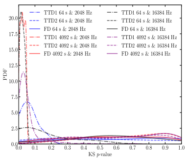
To find an appropriate setting for the TD method, we perform the KS test for the TD and FD methods with different settings. The basic idea of the KS test is to evaluate the credible level at which the whitened noise is consistent with a normal distribution. A KS -value of means that we can exclude the possibility that the tested distribution is not a normal distribution with a confidence level. The higher the -value, the better its match with a normal distribution.
We use two different durations, s and s, and two different sampling rates, Hz and kHz. Normally, we split data into trunks of equal duration, for example, s. Then we average the ACFs or the PSDs that are estimated from these trunks. We also need to truncate the ACF to the duration that we need, for example, s. This indicates that we assume that the duration of the GW signal is enclosed within .
The stationary Gaussian noise follows a multivariate normal distribution, , where is the mean value and is the covariance matrix, which is a Toeplitz matrix based on the ACF. We follow Isi and Farr (2021) to Cholesky-decompose the covariance matrix into a lower-triangular matrix and its transpose ,
| (5) |
The whitened noise can be written as
| (6) |
In the application of KS test, we partitioned the strain data into multiple segments of equivalent duration, specifically s. Consequently, for each method and setting, a set of segmented data was obtained. This allows us to compute an array of -values and establish a distribution derived from the KS test. We discard the truncated data that include the chirp signal, which means that we only calculate the -value for the off-source data. If the ACF describes the noise well, -values follow a rather flat distribution and most of them should be greater than .
In Fig. 1, we show the effect of the total duration and the sampling rate on different methods. The durations of the truncated data are s and s for TD methods and the FD method, respectively. We can see that all the results of the FD method indicate that the PSDs describe the noise well. However, for the results of the TTD1 method, whose truncated ACF is obtained from Eq. (3), almost all of them fail the KS test. For the results of the TTD2 method, whose truncated ACF is obtained from Eq. (4), only the case with a duration of s and a sampling rate of kHz fails the KS test. Compared with the results of Fig. 2, which will be introduced later, it may seem strange that when the total duration is s and the sampling rate is kHz, the results of the TTD2 method do not seem to describe the noise well. We find that this may be caused by the short total duration, because the results become similar to those of the FD cases when we set the total duration to s. This highlights the importance of the total duration , as it affects the estimation of the ACF.
III.2 SNR estimations
Another way to check the consistency among different settings is to compare the SNRs of a GW190521-like signal. First, we generate the waveform in TD, which can be written as where is the time and represents the parameters of the waveform. The source parameters for the SNR calculations are list in Table 1. We use the IMRPhenomXPHM waveform model (Pratten et al., 2021) from LALSuite (LIGO Scientific Collaboration, 2018; Wette, 2020). For TTD methods, it is easy to calculate the SNR based on Eq. (2) and Eq. (5),
| (7) |
For the FD method, we use FFT to transform the TD waveform to FD and then calculate the SNR with
| (8) |
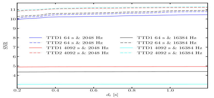
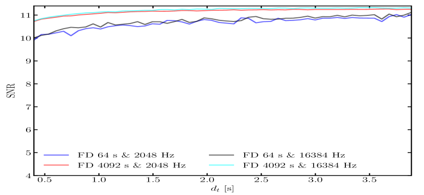
As mentioned above, our GW190521-like event contains the full IMR signal, although the inspiral of which is quite short. So there is no abrupt start or end for this signal and we expect different methods to give the same result. When we calculate SNRs using different methods, the trigger time of the signal always locates in the centre of the data. Furthermore, we take the results of the FD method as the true value, for this method is mature and sufficiently verified. This is also supported by the results in Fig. 1 and Fig. 2.
Moreover we investigate the effect of the duration of the truncated data in Fig. 2, where is also the duration of the signal generated by the waveform model. In Fig. 2, the TTD1 method provides large variance of SNRs. The mean relative error of this method is approximately , indicating potential inadequacies in the handling of ACF estimation within the TTD1 method. In contrast, the Welch method exhibits greater reliability when applied to smaller data sets and demonstrates less susceptibility to nonstationarities.
From Fig. 2, we find that the sampling rate has little effect on the SNRs of a GW190521-like signal. The mean relative errors between the SNRs of the FD method with different sampling rates are all smaller than . For the SNRs of the TTD2 method, the mean relative errors between different sampling rates are smaller than . If we only change the total duration for different methods, the mean relative errors of the SNRs are approximately for TTD2 and FD methods. The results of TTD2 and FD methods show that a larger gives a better estimate of the SNR. The SNRs of the -s long GW data are underestimated compared to the -s long cases. It should be noted that the duration of the trancated data also affects the results of different methods. For these methods, the relative error of SNRs between the smallest and the largest ranges from to .
IV Bayesian inference
We now have a basic idea of how to use the TD method. One of the main points is that it should be performed with sufficiently long durations for both and . Another important point is that the ACF estimated by the TTD1 method may be biased in some improper setting. To further investigate the consistency between two TD methods and the FD method, we compare results of Bayesian inferences from these different methods. Specifically, we use a total duration of GW data s and a sampling rate Hz for TD and FD methods. We select this particular configuration of duration and sampling rate due to its superior performance in both the KS test and SNR comparison, as detailed in Sec. III. Furthermore, this choice aligns with the settings used in Ref. (Wang and Shao, 2023a), demonstrating consistent results across different sampling rates.
The durations of the truncated data are s and s for the TD and FD methods respectively. Note that also represents the duration of the signal generated by the waveform model. On the one hand, the average relative error of the SNRs between the FD method and the TTD2 method is approximately , which is negligible. Thus, we expect similar results from Bayesian inference using these two methods. On the other hand, if one performs Bayesian inference with the biased ACF given by the TTD1 method, we anticipate significantly different results.
In this section, we first introduce the Bayes theorem and some basic settings for Bayesian inference. Then we show results based on more reasonable PSDs, where the PSD is estimated by the PyCBC package.
IV.1 Settings
To estimate the parameters of GW190521 under a specific waveform model , we use the Bayesian inference based on the Bayes theorem,
| (9) |
where is the posteriors of the parameters, is their priors, is the likelihood, and is the evidence. Note that the evidence of a specific model is a constant. According to Finn (1992), the likelihood can be written as,
| (10) | ||||
It is worth noting that, for the TD and FD methods, we calculate the likelihood according to Eq. (2) and Eq. (1), respectively. For multiple detectors, one can simply multiply their likelihoods together.
We impose uniform priors on the redshifted component masses, and we sample from the redshifted chirp mass and the mass ratio in ranges of and , respectively. The prior on the luminosity distance is uniform in the co-moving volume, with a range of Mpc. For other parameters, we use the same priors as those used by the LVK Collaboration (Abbott et al., 2021).
IV.2 Results
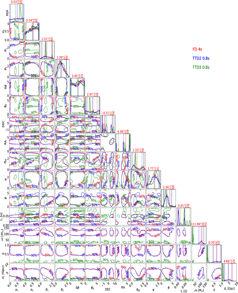
We perform the Bayesian inference using the FD method, the TTD1 method, and the TTD2 method. Note that the downsampling algorithm and the high-pass algorithm used here are implemented in the PyCBC package. We compare posteriors from these three methods in Fig. 3. As expected, the FD method and the TTD2 method give similar posterior distributions for almost all parameters. Furthermore, the log-Bayes factor between them is less than , indicating that we can ignore the differences. We have also tried a duration of s for the truncated ACF of the TTD2 method and obtained similar results.
However, for the TTD1 method, the results are quite different from those of the FD method and the TTD2 method. The estimation of most parameters, such as the chirp-mass and the luminosity distance, seems highly biased. Furthermore, the log-Bayes factor between the TTD1 method and the FD method is . This means that the results from the TTD1 method are very different from the FD and TTD2 methods. This also agrees with what we expected that, a biased ACF due to the improper setting of the TTD1 method leads to biased estimations.
| FD | TTD2 | KLD | JSD | TTD1 | KLD | JSD | Injection | |
|---|---|---|---|---|---|---|---|---|
| [s] | ||||||||
| [] | ||||||||
| [Gpc] |
-
•
*Note: s is the trigger time of GW190521.
The parameter-estimation results are summarised in Table 1. To quantify the differences between the results of those two TTD methods and the FD method, we calculate the Kullback-Leibler divergence (KLD) and the Jensen-Shannon divergence (JSD) between the posterior samples of them. For two posterior distributions and , the KLD of them is defined by
| (11) |
and the JSD of them is defined by
| (12) |
where . As we can see in Table 1, for the TTD2 method, all JSD values are less than , which means that it is acceptable to assume that the difference between the results of these two methods is negligible. However, for the TTD1 method, almost all JSD values are greater than . Thus, we conclude that, given current settings, the TTD1 method gives very different results, compared to the other two methods.
V Discussion and Conclusion
In this paper, we investigate the performance of the TD Bayesian inference. We take the FD Bayesian inference as a comparison when analysing the GW190521 signal, which lasts for only s. This event can be analysed by both the TD and FD methods. Note that such a comparison cannot be made with a ringdown signal alone due to its abrupt start, nor can it currently be performed on a much longer signal due to the computational cost of calculating the inverse of the covariance matrix. For example, for a -s long signal, the dimension of the covariance matrix will be as large as when the sampling rate is Hz. The speed of calculating the likelihood is limited by the computational cost, even if we compute the inverse of the covariance matrix using the Cholesky method.
One of the key points of this investigation is how a truncated ACF can describe the noise as well as a circular ACF does. Therefore, we calculate the KS -values with two truncated ACFs and one circular ACF, which are for the TTD method and the FD method, respectively. We use them to calculate SNRs for a GW190521-like signal generated with the IMRPhenomXPHM waveform model. Compared to the results of the FD method, the results of the TTD2 method are more reliable than those of the TTD1 method. Specifically, the largest relative error between the SNRs of the TTD1 and FD methods is approximately with a non-optimal setting. Furthermore, almost all ACFs for the TTD1 method fail in the KS test. Note that one of the ACFs for the TTD2 method also fails in the KS test when the total duration is not long enough.
The key factors in our comparison are the total duration for the noise estimation, the duration of the truncated data , and the sampling rate . For the total duration , we find that s is not long enough for the analysis of a GW190521-like signal. The relative error caused by this factor can be up to for the TTD2 method. For the sampling rate, its effect is negligible if the adopted total duration is large enough, i.e. s in our case. For the duration of the truncated data , the relative error can be as large as . From these analyses, it is concluded that the TTD2 method should be performed with sufficiently long durations for both and , i.e., s and s for a GW190521-like signal.
To further verify our results, we perform Bayesian inference using two TD methods and the FD method. For two TD methods (TTD1 method and TTD2 method), we set and . For the FD method, we set and . We confirm that, for the TTD2 method and the FD method, they have similar results, and the log-Bayes factor between their posteriors is less than . The JSD values of each parameter between these two methods are all less than , meaning that the difference between them is negligible.
For the TTD1 method and the FD method, the log-Bayes factor between them is about , and the JSD values of most parameters are larger than . However, we cannot conclude that the TTD1 method itself is not reliable. It is posited that consistent outcomes can be achieved given the correct handling of the data. This assertion is substantiated by Fig. 1 and Fig. 2, which illustrate results obtained from a total duration of s at a sampling rate of Hz, demonstrating consistency between the TTD1 method and the FD method. The reliability of the TTD1 method under different settings can further be verified through a KS test, as detailed in Sec. III.1. We do not delve deeply into this since the TTD2 method is both reliable and accessible. We here aim to present results of the biased TTD1 method for comparison. Overall, this analysis highlights the importance of performing the consistency check between different methods.
The TTD method is widely used in ringdown analysis. Here, we show that it can also be used in the full IMR analysis only when we handle it with extra care. Furthermore, our analyses are helpful to understand the inconsistency between the results of Ref. (Isi et al., 2021) and Ref. (Cotesta et al., 2022). Based on our analyses, we got consistent results for ringdown analyses of GW150914 with different sampling frequencies, as shown in Ref. (Wang and Shao, 2023a). To allow for reproducibility, we have released codes for noise estimation at Ref. (Wang and Shao, 2023b).
Acknowledgements.
We thank Yi-Ming Hu for insightful discussions and the anonymous referee for constructive comments. This work was supported by the China Postdoctoral Science Foundation (2022TQ0011), the National Natural Science Foundation of China (12247152, 11975027, 11991053, 11721303), the National SKA Program of China (2020SKA0120300), the Beijing Municipal Natural Science Foundation (1242018), the Max Planck Partner Group Program funded by the Max Planck Society, and the High-performance Computing Platform of Peking University. HTW is supported by the Opening Foundation of TianQin Research Center. This research has made use of data or software obtained from the Gravitational Wave Open Science Center (gwosc.org), a service of LIGO Laboratory, the LIGO Scientific Collaboration, the Virgo Collaboration, and KAGRA Abbott et al. (2023b). LIGO Laboratory and Advanced LIGO are funded by the United States National Science Foundation (NSF) as well as the Science and Technology Facilities Council (STFC) of the United Kingdom, the Max-Planck-Society (MPS), and the State of Niedersachsen/Germany for support of the construction of Advanced LIGO and construction and operation of the GEO600 detector. Additional support for Advanced LIGO was provided by the Australian Research Council. Virgo is funded, through the European Gravitational Observatory (EGO), by the French Centre National de Recherche Scientifique (CNRS), the Italian Istituto Nazionale di Fisica Nucleare (INFN) and the Dutch Nikhef, with contributions by institutions from Belgium, Germany, Greece, Hungary, Ireland, Japan, Monaco, Poland, Portugal, Spain. KAGRA is supported by Ministry of Education, Culture, Sports, Science and Technology (MEXT), Japan Society for the Promotion of Science (JSPS) in Japan; National Research Foundation (NRF) and Ministry of Science and ICT (MSIT) in Korea; Academia Sinica (AS) and National Science and Technology Council (NSTC) in Taiwan of China.References
- Isi and Farr (2022) M. Isi and W. M. Farr, arXiv e-prints , arXiv:2202.02941 (2022), arXiv:2202.02941 [gr-qc] .
- Abbott et al. (2019) B. P. Abbott et al. (LIGO Scientific Collaboration and Virgo Collaboration), Phys. Rev. X 9, 031040 (2019).
- Abbott et al. (2021) R. Abbott et al., Phys. Rev. X 11, 021053 (2021), arXiv:2010.14527 [gr-qc] .
- Abbott et al. (2023a) R. Abbott et al. (KAGRA, VIRGO, LIGO Scientific), Phys. Rev. X 13, 041039 (2023a), arXiv:2111.03606 [gr-qc] .
- Abbott et al. (2020) B. P. Abbott et al. (LIGO Scientific, Virgo), Class. Quant. Grav. 37, 055002 (2020), arXiv:1908.11170 [gr-qc] .
- Isi and Farr (2021) M. Isi and W. M. Farr, arXiv e-prints , arXiv:2107.05609 (2021), arXiv:2107.05609 [gr-qc] .
- Vishveshwara (1970) C. V. Vishveshwara, Phys. Rev. D 1, 2870 (1970).
- Press (1971) W. H. Press, Astrophys. J. Lett. 170, L105 (1971).
- Teukolsky (1973) S. A. Teukolsky, Astrophys. J. 185, 635 (1973).
- Finch and Moore (2021) E. Finch and C. J. Moore, Phys. Rev. D 104, 123034 (2021), arXiv:2108.09344 [gr-qc] .
- Finch and Moore (2022) E. Finch and C. J. Moore, Phys. Rev. D 106, 043005 (2022), arXiv:2205.07809 [gr-qc] .
- Bustillo et al. (2021) J. C. Bustillo, P. D. Lasky, and E. Thrane, Phys. Rev. D 103, 024041 (2021).
- Capano et al. (2022) C. D. Capano, J. Abedi, S. Kastha, A. H. Nitz, J. Westerweck, Y.-F. Wang, M. Cabero, A. B. Nielsen, and B. Krishnan, (2022), arXiv:2209.00640 [gr-qc] .
- Isi et al. (2021) M. Isi, W. M. Farr, M. Giesler, M. A. Scheel, and S. A. Teukolsky, Phys. Rev. Lett 127, 011103 (2021), arXiv:2012.04486 [gr-qc] .
- Cotesta et al. (2022) R. Cotesta, G. Carullo, E. Berti, and V. Cardoso, Phys. Rev. Lett 129, 111102 (2022), arXiv:2201.00822 [gr-qc] .
- Abbott et al. (2016) B. P. Abbott et al. (LIGO Scientific Collaboration and Virgo Collaboration), Phys. Rev. Lett. 116, 061102 (2016).
- Abbott et al. (2020) R. Abbott et al. (LIGO Scientific Collaboration and Virgo Collaboration), Phys. Rev. Lett 125, 101102 (2020), arXiv:2009.01075 [gr-qc] .
- Isi et al. (2019) M. Isi, M. Giesler, W. M. Farr, M. A. Scheel, and S. A. Teukolsky, Phys. Rev. Lett 123, 111102 (2019), arXiv:1905.00869 [gr-qc] .
- Abbott et al. (2021a) R. Abbott et al. (LIGO Scientific, Virgo), Phys. Rev. D 103, 122002 (2021a), arXiv:2010.14529 [gr-qc] .
- Abbott et al. (2021b) R. Abbott et al. (LIGO Scientific, VIRGO, KAGRA), arXiv e-prints , arXiv:2112.06861 (2021b), arXiv:2112.06861 [gr-qc] .
- Wang et al. (2021) H.-T. Wang, S.-P. Tang, P.-C. Li, and Y.-Z. Fan, Phys. Rev. D 104, 104063 (2021), arXiv:2104.07594 [gr-qc] .
- Cheung et al. (2021) M. H.-Y. Cheung, L. W.-H. Poon, A. K.-W. Chung, and T. G. F. Li, JCAP 02, 040 (2021), arXiv:2002.01695 [gr-qc] .
- Mishra et al. (2022) A. K. Mishra, A. Ghosh, and S. Chakraborty, Eur. Phys. J. C 82, 820 (2022), arXiv:2106.05558 [gr-qc] .
- Hu et al. (2021) P. Hu, K. Jani, K. Holley-Bockelmann, and G. Carullo, (2021), arXiv:2112.06856 [gr-qc] .
- Punturo et al. (2010) M. Punturo, M. Abernathy, et al., Class. Quantum Grav. 27, 194002 (2010).
- Reitze et al. (2019) D. Reitze, R. X. Adhikari, et al., in Bull. Am. Astron. Soc., Vol. 51 (2019) p. 35, arXiv:1907.04833 [astro-ph.IM] .
- Amaro-Seoane et al. (2017) P. Amaro-Seoane, H. Audley, S. Babak, J. Baker, et al., ArXiv e-prints , arXiv:1702.00786 (2017), arXiv:1702.00786 [astro-ph.IM] .
- Luo et al. (2016) J. Luo et al. (TianQin), Class. Quant. Grav. 33, 035010 (2016), arXiv:1512.02076 [astro-ph.IM] .
- Mei et al. (2021) J. Mei et al. (TianQin), PTEP 2021, 05A107 (2021), arXiv:2008.10332 [gr-qc] .
- Hu and Wu (2017) W.-R. Hu and Y.-L. Wu, National Science Review 4, 685 (2017).
- Allen et al. (2012) B. Allen, W. G. Anderson, P. R. Brady, D. A. Brown, and J. D. E. Creighton, Phys. Rev. D 85, 122006 (2012), arXiv:gr-qc/0509116 [gr-qc] .
- Khan and Agha (2020) M. Khan and S. Agha, Analog Integrated Circuits and Signal Processing 105, 99 (2020).
- Welch (1967) P. D. Welch, IEEE Trans. Audio & Electroacoust 15 (1967), 10.1109/TAU.1967.1161901.
- Pratten et al. (2021) G. Pratten, C. García-Quirós, M. Colleoni, A. Ramos-Buades, H. Estellés, M. Mateu-Lucena, R. Jaume, M. Haney, D. Keitel, J. E. Thompson, and S. Husa, Phys. Rev. D 103, 104056 (2021), arXiv:2004.06503 [gr-qc] .
- LIGO Scientific Collaboration (2018) LIGO Scientific Collaboration, “LIGO Algorithm Library - LALSuite,” free software (GPL) (2018).
- Wette (2020) K. Wette, SoftwareX 12, 100634 (2020).
- Wang and Shao (2023a) H.-T. Wang and L. Shao, Phys. Rev. D 108, 123018 (2023a), arXiv:2311.13300 [gr-qc] .
- Finn (1992) L. S. Finn, Phys. Rev. D46, 5236 (1992), arXiv:gr-qc/9209010 [gr-qc] .
- Ashton et al. (2019) G. Ashton et al., ApJS 241, 27 (2019).
- Speagle (2020) J. S. Speagle, MNRAS 493, 3132 (2020), arXiv:1904.02180 [astro-ph.IM] .
- Wang and Shao (2023b) H. Wang and L. Shao, , (2023b).
- Abbott et al. (2023b) R. Abbott et al. (KAGRA, VIRGO, LIGO Scientific), Astrophys. J. Suppl. 267, 29 (2023b), arXiv:2302.03676 [gr-qc] .