Reinforcement Learning with Hidden Markov Models for Discovering Decision-Making Dynamics

Abstract

Major depressive disorder (MDD), a leading cause of years of life lived with disability, presents challenges in diagnosis and treatment due to its complex and heterogeneous nature. Emerging evidence indicates that reward processing abnormalities may serve as a behavioral marker for MDD. To measure reward processing, patients perform computer-based behavioral tasks that involve making choices or responding to stimulants that are associated with different outcomes, such as gains or losses in the laboratory. Reinforcement learning (RL) models are fitted to extract parameters that measure various aspects of reward processing (e.g., reward sensitivity) to characterize how patients make decisions in behavioral tasks. Recent findings suggest the inadequacy of characterizing reward learning solely based on a single RL model; instead, there may be a switching of decision-making processes between multiple strategies. An important scientific question is how the dynamics of learning strategies in decision-making affect the reward learning ability of individuals with MDD. Motivated by the probabilistic reward task (PRT) within the EMBARC study, we propose a novel RL-HMM framework for analyzing reward-based decision-making. Our model accommodates learning strategy switching between two distinct approaches under a hidden Markov model (HMM): subjects making decisions based on the RL model or opting for random choices. We account for continuous RL state space and allow time-varying transition probabilities in the HMM. We introduce a computationally efficient EM algorithm for parameter estimation and employ a nonparametric bootstrap for inference. Extensive simulation studies validate the finite-sample performance of our method. We apply our approach to the EMBARC study to show that MDD patients are less engaged in RL compared to the healthy controls, and engagement is associated with brain activities in the negative affect circuitry during an emotional conflict task. reinforcement learning; reward tasks; state-switching; behavioral phenotyping; mental health; brain-behavior association

1 Introduction

Despite extensive research and clinical efforts dedicated to developing pharmacological and behavioral treatments for mental disorders over the years, a significant setback is symptom-based diagnoses that assume discrete disease categories, which may contribute to low remission rates and inadequate treatment responses as it does not fully account for the heterogeneity and complexity of mental disorders (Rush et al., 2006). In response to the limitations inherent in traditional symptom-based diagnoses and to address significant between-patient heterogeneity, the National Institute of Mental Health (NIMH) advocates for a paradigm shift through the Research Domain Criteria (RDoC) initiative (Insel et al., 2010). This shift involves redefining mental disorders by identifying latent constructs derived from biological and behavioral measures across diverse domains of functioning (e.g., positive/negative affect, decision-making, social processing) at different levels (e.g., cells, genes, and brain circuits), instead of solely relying on the clinical symptoms. Behavioral data collected from tasks such as the probabilistic reward task (PRT; Pizzagalli et al., 2005) and the emotion conflict task (Etkin et al., 2006) is a highly valued resource within the framework of RDoC. Utilizing carefully designed behavioral tasks with appropriate data- or theory-driven computational methods (Huys et al., 2016), researchers can extract valuable behavioral markers that serve as indicators of mental health conditions. Moreover, there is a critical need to examine the associations between the brain and behavior, as demonstrated by Fonzo et al. (2019). This exploration facilitates understanding the underlying brain mechanisms during behavioral tasks, allowing for the identification of brain abnormalities related to mental disorders, and ultimately contributes to refining diagnostic frameworks and developing more effective therapeutic interventions.

Reward learning and decision-making are pivotal in the etiology of mental function (Kendler et al., 1999). Reward processing refers to how individuals perceive, value, and pursue rewards (e.g., money, social approval). MDD patients may show abnormalities in reward processing, such as reduced motivation, anhedonia (loss of pleasure), or reduced sensitivity to positive rewards. To measure reward processing, patients perform computer-based behavioral tasks that involve making choices or responding to stimulants that are associated with different outcomes, such as gains or losses in the laboratory. We focus on characterizing human decision-making behaviors through reward tasks (e.g., PRT), wherein individuals make decisions by interacting with a reward-based system and continually adapting their decision-making mechanisms based on obtained rewards.

Biological evidence suggests that fluctuations in human dopaminergic neurons indicate errors in predicting future rewarding events (Schultz et al., 1997). This supports the use of simple prediction error learning (comparing real and expected reward) to update the value functions of different choices (Rescorla, 1972; Huys et al., 2011), laying the foundation for modeling behavior by Reinforcement Learning (RL; Sutton and Barto, 2018). To describe reward learning behaviors emerging from a reward learning task, Huys et al. (2013) introduced a prediction error RL approach to characterize decision making based on key behavioral phenotypes, including reward sensitivity and learning rate. In a PRT study, they identified reward sensitivity (instead of learning rate) as an important behavioral marker contributing to the abnormality in reward learning for MDD, with a lower reward sensitivity in MDD patients. Guo et al. (2023) extends the approach of Huys et al. (2013) to a more general semiparametric RL framework by replacing the scalar value of reward sensitivity with a nonlinear and nondecreasing reward sensitivity function. They revealed that the reward sensitivity for the MDD patients is not uniformly lower than the healthy subjects, but only when subjects receive sufficient rewards.

Furthermore, Guo et al. (2023) noted a floor and ceiling effect in the relationship between choices and expected rewards, attributed to the non-linearity of the reward sensitivity function, indicating that the decision-making process may not adhere to a single RL model. Several other studies also support that subjects employ multiple learning strategies in decision-making, as highlighted by Worthy et al. (2013); Iigaya et al. (2018); Ashwood et al. (2022). In particular, Ashwood et al. (2022) demonstrates that the perceptual decision-making process switches between multiple interleaved strategies. They suggest that the decision process involves a mixture of ‘engaged’ and ‘lapse’ strategies. During the ‘engaged’ strategy, a subject makes choices following a generalized linear model with softmax. Conversely, during the ‘lapse’ strategy, the subject ignores the stimulus and makes choices based on a fixed probability. The dynamics of strategy-switching are modeled by a hidden Markov model (HMM). Alternatively, Chen et al. (2021) considers ‘engaged’ as exploitation and ‘lapse’ as exploration, aligning with the exploitation-exploration trade-off in RL (Sutton and Barto, 2018). During the exploration stages, each choice is assigned equal probabilities.

In this work, we propose an RL-HMM framework to characterize reward-based decision-making with alternating learning strategies between two distinct decision-making processes: in the ‘engaged’ state, subjects make decisions based on the RL model, while in the ‘lapse’ state, subjects make decisions through random choices with equal probabilities. Our approach generalizes the RL model introduced in Huys et al. (2013) and Guo et al. (2023) from finite discrete RL states to infinite but bounded state space. We employ HMM with time-varying transition probabilities to model the learning strategy switching, extending the HMM framework in Ashwood et al. (2022), where the transition probabilities are assumed to be time-invariant. In our approach, the time-varying transition probabilities are modeled nonparametrically with fused lasso regularization (Tibshirani et al., 2005) or trend filtering (Tibshirani, 2014). The proposed approach is applied to the Probabilistic Reward Task (Pizzagalli et al., 2005) in the EMBARC study (Trivedi et al., 2016), a large-scale randomized clinical trial recruiting participants diagnosed with MDD and healthy controls (details in Section 4.1).

The remainder of the article is organized as follows. Section 2 introduces a general RL model with an approximate solution, outlines our RL-HMM method, and provides details on parameter estimation, inference, and model selection. In Section 3, we present results from our simulation studies, while Section 4 focuses on the analysis of PRT data from the EMBARC study. In Section 5, we summarize our approach, highlight key findings, and discuss potential extensions for future research.

2 Methods

Consider a group of $n$ subjects. The dataset comprises decision-making processes of each subject, (i.e., $\dots,S_{it}\rightarrow A_{it}\rightarrow R_{it}\rightarrow S_{it+1}\rightarrow A_{it+1}\rightarrow R_{it+1},\dots$), where $S_{it}$, $A_{it}$, and $R_{it}$ represent the random variables of state, action, and reward for the $i$-th subject at time $t$, respectively. Throughout this paper, we assume that the states reside within a bounded state space denoted as $\mathcal{S}$. We consider a discrete action space $\mathcal{A}$ with $D$ available options (i.e. $\mathcal{A}=\{0,1,\dots,D-1\}$). The reward $R_{it}$ is generated based on a function involving $S_{it}$, $A_{it}$, and $t$. We assume that $R_{it}$ is bounded and can be discrete or continuous. In the task of modeling human reward learning abilities in behavioral experiments, rewards are provided without delay.

2.1 Decision-making with reinforcement learning

Reinforcement Learning (RL) is a computational framework that can be used to model subjects’ responses to rewards in behavioral tasks. In this framework, subjects learn the underlying reward generating mechanism and subsequently make decisions based on their acquired knowledge.

Define $Q_{i}^{t}(a,s)$ as the expected reward for taking action $a$ at state $s$ for the $i$th participant at the $t$th trial. Assume that the expected reward can be approximated by $\widetilde{Q}_{i}^{t}(a,s)=\bm{\phi}(a,s)^{\top}\bm{\delta}_{i}^{t}$, where $\bm{\phi}(a,s)$ represents the basis vector associated with the state $s\in\mathcal{S}$ for action $a\in\mathcal{A}$. After observing the reward $R_{it}=r_{it}$ at trial $t$, the participant updates the expected reward $\widetilde{Q}_{i}^{t}(a,s)$ by adjusting it in the direction of $r_{it}-\widetilde{Q}_{i}^{t}(a,s)$. The corresponding update of the coefficients follows:

$$\bm{\delta}_{i}^{t+1}=\bm{\delta}_{i}^{t}+\beta\bm{\phi}(a_{it},s_{it})\left[r_{it}-\bm{\phi}(a_{it},s_{it})^{\top}\bm{\delta}_{i}^{t}\right],$$ (1)

where $\beta$ is the learning rate. Note that (1) is also known as the Rescorla-Wagner equation (Rescorla, 1972). It can be viewed as a one-step stochastic gradient descent, where we minimize the risk associated with the following mean squared error:

$$\mathbb{E}_{R}\left[\left(R_{it}-\bm{\phi}(a_{it},s_{it})^{\top}\bm{\delta}_{i}^{t}\right)^{2}\ \bigl{|}\ A_{it}=a_{it},S_{it}=s_{it}\right].$$ (2)

Left multiplying $\phi^{\top}(a_{it},s_{it})$ to both sides of (1), we obtain

$$Q_{i}^{t+1}(a_{it},s_{it})=\beta_{it}r_{it}+(1-\beta_{it})Q_{i}^{t}(a_{it},s_{it}),$$ (3)

where $\beta_{it}=\beta\bm{\phi}(a_{it},s_{it})^{\top}\bm{\phi}(a_{it},s_{it})$. To ensure that the expected reward at $t+1$ is the weighted sum of the obtained reward and the expected reward at $t$, the learning rate should satisfy $0<\beta_{it}<1$. As a note, if $s$ is discrete and we choose $\phi(a,s)$ as indicator functions on all discrete values in $\mathcal{A}\times\mathcal{S}$, then $\bm{\phi}(a_{it},s_{it})^{\top}\bm{\phi}(a_{it},s_{it})\equiv 1$ and $\beta_{it}\equiv\beta$ in (3). Alternatively, if $s$ is continuous, we choose $\phi(a,s)=(I(a=0),I(a=1))^{\top}\otimes\psi(s)$, where $\psi(s)$ can be a linear basis or B-splines. We further assume that $\bm{\alpha}:=\bm{\delta}^{1}=\bm{\delta}_{i}^{1}$. Define $\mathcal{H}_{it}=\{S_{ij},A_{ij},R_{ij}\}_{j=1}^{t-1}$ as the observed history for the $i$-th subject up to time $t$. We assume that the action $A_{it}$ follows the model

$$P\left(A_{it}=a\mid S_{it},\mathcal{H}_{it}\right)=\frac{\exp\{\nu_{a}+\rho Q_{i}^{t}(a,S_{it})\}}{\sum_{a^{\prime}=0}^{D-1}\exp\{\nu_{a^{\prime}}+\rho Q_{i}^{t}(a^{\prime},S_{it})\}},$$ (4)

where $\rho>0$ is the reward sensitivity. A higher reward sensitivity indicates that subjects’ actions will depend more on the expected rewards they learned. Here, $\nu_{a}$ $(a=0,\dots,D-1)$ are time-invariant intercepts. To ensure identifiability, we let $\nu_{0}\equiv 0$, and $\nu_{1}=\dots=\nu_{D-1}=0$ implies that the subject is making decisions entirely based on the expected reward.

2.2 Decision-making with state switching learning strategies

Several studies provide evidence that subjects employ multiple learning strategies for decision-making (Worthy et al., 2013; Iigaya et al., 2018; Ashwood et al., 2022). In this work, we consider that subjects exhibit two distinct learning strategies: the ‘engaged’ state (represented as $U_{it}=1$), in which subjects make decisions based on the RL model (Huys et al., 2013; Guo et al., 2023), and the ‘lapse’ state (represented as $U_{it}=0$), where subjects make decisions through random choices, with an equal probability of $1/D$ for selecting one of the $D$ available actions (Chen et al., 2021). Here, $U_{it}\in\{0,1\}$ represents a latent variable that indicates the learning strategy used by the subject $i$ during trial $t$. We introduce a novel RL-HMM framework for the analysis of perceptual decision-making behavior, employing a combination of hidden Markov model (HMM) and reinforcement learning. The proposed RL-HMM model is:

$$P\left(A_{it}=a\mid U_{it},S_{it},\mathcal{H}_{it}\right) =I(U_{it}=1)\frac{\exp\{\nu_{a}+\rho Q_{i}^{t}(a,S_{it})\}}{\sum_{a^{\prime}=0}^{D-1}\exp\{\nu_{a^{\prime}}+\rho Q_{i}^{t}(a^{\prime},S_{it})\}}+I(U_{it}=0)\frac{1}{D},$$ (5)

$$P\left(U_{i,t+1}=1\mid U_{it}=j\right) =\frac{\exp(\zeta_{jt})}{1+\exp(\zeta_{jt})}\quad j=0,1.$$ (6)

Here, $\zeta_{jt}=\zeta_{j}(t)$ represents a nonparametric function indicating that the transition probability may vary across trials. The learning strategy at the initial trial is characterized by the probability distribution $P\left(U_{i1}=j\right)=\pi_{j}$, where $0<\pi_{0},\pi_{1}<1$, and $\pi_{0}+\pi_{1}=1$.

2.3 Parameter estimation via EM algorithm

In the proposed model, denote $\bm{\theta}=\left\{\beta,\rho,\nu_{1},\dots,\nu_{D-1},\bm{\alpha},\pi_{1},\bm{\zeta}_{0},\bm{\zeta}_{1}\right\}$ as the parameters of interest, where $\bm{\zeta}_{j}=\zeta_{j,[1:T-1]}$. Define $\mathbf{A}_{i}=(A_{i1},\dots,A_{iT})$ (a similar definition applied to $\mathbf{S}_{i},\mathbf{R}_{i}$ and $\mathbf{U}_{i}$). Since $R_{it}$ and $S_{it}$ given ${\cal H}_{it}$ are independent of $\bm{\theta}$, it is sufficient to consider the joint distribution of $(\mathbf{A}_{1:n},\mathbf{U}_{1:n})$ condition on $(\mathbf{S}_{1:n},\mathbf{R}_{1:n})$ to estimate $\bm{\theta}$ without modeling the distribution of $(\mathbf{S}_{1:n},\mathbf{R}_{1:n})$. The joint likelihood, denoted as $\mathcal{L}$, can be expressed by

$$\mathcal{L}\left(\bm{\theta};\mathbf{A}_{1:n},\mathbf{U}_{1:n}\right) =\sum_{i=1}^{n}\bigg{(}\log P(U_{i1})+\sum_{t=1}^{T-1}\log P\left(U_{i,t+1}\mid U_{it}\right)+\sum_{t=1}^{T}\log P\left(A_{it}\mid U_{it},S_{it},\mathcal{H}_{it}\right)\bigg{)}.$$

To avoid overfitting, we regularize $\bm{\zeta}_{j}$ via trend filtering penalty (Tibshirani, 2014)

$$\lambda_{0}\left\|\mathbf{D}^{(r+1)}\bm{\zeta}_{0}\right\|_{1}+\lambda_{1}\left\|\mathbf{D}^{(r+1)}\bm{\zeta}_{1}\right\|_{1},$$

where $\mathbf{D}^{(r+1)}\in\mathbb{R}^{(T-r-2)\times(T-1)}$ is the discrete difference operator of order $r$. When $r=0$, we have

$$\mathbf{D}^{(1)}=\left[\begin{array}[]{cccccc}-1&1&0&\cdots&0&0\\ 0&-1&1&\cdots&0&0\\ \vdots&&&&&\\ 0&0&0&\cdots&-1&1\end{array}\right]\in\mathbb{R}^{(T-2)\times(T-1)},$$

and the zero-th order trend filtering problem reduces to one-dimensional fused Lasso (Tibshirani et al., 2005). For $r\geq 1$, $\mathbf{D}^{(r+1)}$ is defined recursively by

$$\mathbf{D}^{(r+1)}=\mathbf{D}_{r}^{(1)}\cdot\mathbf{D}^{(r)},$$

where $\mathbf{D}_{r}^{(1)}$ is the $(T-r-2)\times(T-r-1)$ version of $\mathbf{D}^{(1)}$. When $r=0$ and $\lambda_{0},\lambda_{1}\rightarrow\infty$, the estimated HMM will have fixed transition probabilities for all trials. We estimate $\bm{\theta}$ by the Expectation Maximization (EM) algorithm.

E-step: The E-step involves computing the posterior distribution of $U_{it}$, which is challenging due to the HMM structure. The forward-backward algorithm (Baum et al., 1970; Ashwood et al., 2022) addresses the challenge by employing recursion and memoization, with both the forward pass and backward pass of the algorithm requiring just a single traversal through all trials within a session. Specifically, we first compute the expectation of $\mathcal{L}\left(\bm{\theta};\mathbf{A}_{1:n},\mathbf{U}_{1:n}\right)$ in terms of $P(\mathbf{U}_{1:n}\mid\mathbf{A}_{1:n},\bm{\theta}^{\mbox{old}})$:

$$\mathrm{E}_{U}\left(\mathcal{L}\left(\bm{\theta};\mathbf{A}_{1:n},\mathbf{U}_{1:n}\right)\mid\mathbf{A}_{1:n},\bm{\theta}^{\mbox{old}}\right) =\sum_{i=1}^{n}\Bigg{\{}\sum_{j=0}^{1}\gamma_{ij1}(\bm{\theta}^{\mbox{old}})\cdot\log\pi_{j}+\sum_{t=1}^{T-1}\sum_{j=0}^{1}\sum_{k=0}^{1}\xi_{ijkt}(\bm{\theta}^{\mbox{old}})\cdot\log C_{jk}^{t}$$

$$+\sum_{t=1}^{T}\sum_{j=0}^{1}\gamma_{ijt}(\bm{\theta}^{\mbox{old}})\cdot\log P\left(A_{it}\mid U_{it}=j,S_{it},\mathcal{H}_{it}\right)\Bigg{\}},$$ (7)

$\gamma_{ijt}$, $\xi_{ijkt}$, and $C_{jk}^{t}$ are defined by

$$\gamma_{ijt}=\gamma_{ijt}(\bm{\theta})=P\left(U_{it}=j\mid\mathbf{A}_{i},\bm{\theta}\right),\quad\xi_{ijkt}=\xi_{ijkt}(\bm{\theta})=P\left(U_{i,t+1}=k,U_{it}=j\mid\mathbf{A}_{i},\bm{\theta}\right),$$

$$C^{t}_{jk}=C^{t}_{jk}(\bm{\theta})=P\left(U_{i,t+1}=k\mid U_{it}=j,\bm{\theta}\right).$$

Define $a_{ijt}=P\left(U_{it}=j,\mathbf{A}_{i,[1:t]}\right)$, $\eta_{ijt}=P\left(A_{it}\mid U_{it}=j,S_{it},\mathcal{H}_{it}\right)$, we can compute the value of $a_{ijt}$ through forward passing with $a_{ij1}=\pi_{j}\eta_{ij1}$ and

$$a_{ijt} =\sum_{k=0}^{1}P\left(U_{it}=j,U_{i,t-1}=k,\mathbf{A}_{i,[1:t-1]},A_{it}\right)$$

$$=\sum_{k=0}^{1}P\left(U_{i,t-1}=k,\mathbf{A}_{i,[1:t-1]}\right)P\left(A_{it}\mid U_{it}=j,\mathbf{A}_{i,[1:t-1]}\right)P\left(U_{it}=j\mid U_{i,t-1}=k\right)$$

$$=\sum_{k=0}^{1}a_{ik,t-1}\eta_{ijt}C_{kj}^{t-1},\quad\mbox{for}\ t>1$$

Define $b_{ijt}=P\left(\mathbf{A}_{i,[t+1:T]}\mid U_{it}=j,\mathbf{A}_{i,[1:t]}\right)$, we can compute the value of $b_{ijt}$ through backward passing with $b_{ijT}=1$ and

$$b_{ijt} =\sum_{k=0}^{1}P\left(A_{i,t+1},\mathbf{A}_{i,[t+2:T]},U_{i,t+1}=k\mid U_{it}=j,\mathbf{A}_{i,[1:t]}\right)$$

$$=\sum_{k=0}^{1}P\left(\mathbf{A}_{i,[t+2:T]}\mid U_{i,t+1}=k,\mathbf{A}_{i,[1:t+1]}\right)P\left(A_{i,t+1}\mid U_{i,t+1}=k,\mathbf{A}_{i,[1:t]}\right)P\left(U_{i,t+1}=k\mid U_{it}=j\right)$$

$$=\sum_{k=0}^{1}b_{ik,t+1}\eta_{ik,t+1}C_{jk}^{t},\quad\mbox{for}\ t<T$$

The above derivation of $a_{ijt}$ and $b_{ijt}$ uses the Markov property of $U_{it}$. Then we compute

$$\gamma_{ijt} =\frac{P\left(U_{it}=j,\mathbf{A}_{i,[1:t]}\right)P\left(\mathbf{A}_{i,[t+1:T]}\mid U_{it}=j,\mathbf{A}_{i,[1:t]}\right)}{P\left(\mathbf{A}_{i}\right)}=\frac{a_{ijt}b_{ijt}}{\sum_{k=0}^{1}a_{ikT}}$$

Similarly, we have

$$\xi_{ijkt} =\frac{P\left(U_{i,t+1}=k,U_{it}=j,\mathbf{A}_{i,[1:t]},\mathbf{A}_{i,[t+1:T]}\right)}{P\left(\mathbf{A}_{i}\right)}=\frac{a_{ijt}b_{ik,t+1}\eta_{ik,t+1}C_{jk}^{t}}{\sum_{k=0}^{1}a_{ikT}}$$

M-step: write the objective function as follow:

$$\mathcal{J}_{\bm{\lambda}}\left(\bm{\theta}\right) =-\mathrm{E}_{U}\left(\mathcal{L}\left(\bm{\theta};\mathbf{A}_{1:n},\mathbf{U}_{1:n}\right)\mid\mathbf{A}_{1:n},\bm{\theta}^{\mbox{old}}\right)+\sum_{j=0}^{1}\lambda_{j}\left\|\mathbf{D}^{(r+1)}\bm{\zeta}_{j}\right\|_{1},$$ (8)

where $\bm{\lambda}=(\lambda_{0},\lambda_{1})$. From (7), we find that we can partition $\mathcal{J}_{\bm{\lambda}}\left(\bm{\theta}\right)$ into four components that only contain $\pi_{1}$, $\bm{\zeta}_{0}$, $\bm{\zeta}_{1}$, $(\beta,\rho,\nu_{1},\dots,\nu_{D-1},\bm{\alpha})$, respectively. Each part is minimized separately. We apply the generalized EM algorithm (Dempster et al., 1977), where we replace the minimization step with a one-step update of Newton’s method. At the $(l+1)$-th iteration, we update the parameter estimates as follows:

Update $\pi_{1}$: ${\pi_{1}}^{(l+1)}=n^{-1}\sum_{i=1}^{n}\gamma_{i11}(\bm{\theta}^{(l)})$.

Update $\bm{\zeta}_{j}$ $(j=0,1)$: Define $\xi_{ijkt}^{(l)}=\xi_{ijkt}(\bm{\theta}^{(l)})$ write (8) in terms of $\bm{\zeta}_{j}$

$$\mathcal{J}_{\lambda_{j}}\left(\bm{\zeta}_{j}\right) =\sum_{i=1}^{n}\sum_{t=1}^{T-1}\bigg{\{}-\xi_{ij1t}^{(l)}\zeta_{jt}+\left(\xi_{ij0t}^{(l)}+\xi_{ij1t}^{(l)}\right)\log\left(1+\exp\left(\zeta_{jt}\right)\right)\bigg{\}}+\lambda_{j}\left\|\mathbf{D}^{(r+1)}\bm{\zeta}_{j}\right\|_{1}.$$

When $\lambda_{j}=0$, the gradient and Hessian matrix of $\mathcal{J}_{0}$ in terms of $\bm{\zeta}_{j}$ can be represented by

$$\mathbf{g}_{0}(\bm{\zeta}_{j})=(g_{0}(\zeta_{j1}),\dots,g_{0}(\zeta_{j,T-1}))^{\top}\quad\mbox{where}\quad g_{0}(\zeta_{jt})=\sum_{i=1}^{n}\Big{\{}-\xi_{ij1t}^{(l)}+\left(\xi_{ij0t}^{(l)}+\xi_{ij1t}^{(l)}\right)C_{j1}^{t}\Big{\}}$$

$$\mathbf{H}_{0}(\bm{\zeta}_{j})=\mbox{diag}(H_{0}(\zeta_{j1}),\dots,H_{0}(\zeta_{j,T-1}))\quad\mbox{where}\quad H_{0}(\zeta_{jt})=\sum_{i=1}^{n}\left(\xi_{ij0t}^{(l)}+\xi_{ij1t}^{(l)}\right)C_{j1}^{t}(1-C_{j1}^{t}).$$

We can update $\bm{\zeta}_{j}$ by one Newton-Raphson step

$$\bm{\zeta}_{j}^{(l+1)}=\bm{\zeta}_{j}^{(l)}-\mathbf{H}_{0}^{-1}(\bm{\zeta}_{j}^{(l)})\mathbf{g}_{0}(\bm{\zeta}_{j}^{(l)}).$$ (9)

Approximate $\mathcal{J}_{0}(\bm{\zeta}_{j})$ by taking its second-order Taylor expansion around $\bm{\zeta}_{j}^{(l)}$:

$$\mathcal{J}_{0}(\bm{\zeta}_{j}^{(l)})+\sum_{t=1}^{T-1}g_{0}(\zeta_{jt}^{(l)})\left(\zeta_{jt}-\zeta_{jt}^{(l)}\right)+\frac{1}{2}\sum_{t=1}^{T-1}H_{0}(\zeta_{jt}^{(l)})\left(\zeta_{jt}-\zeta_{jt}^{(l)}\right)^{2}$$

$$= \frac{1}{2}\sum_{t=1}^{T-1}H_{0}(\zeta_{jt}^{(l)})\left(\zeta_{jt}-\zeta_{jt}^{(l)}+H_{0}^{-1}(\zeta_{jt}^{(l)})g_{0}(\zeta_{jt}^{(l)})\right)^{2}+\mbox{Const.},$$ (10)

it is easy to show that updating $\bm{\zeta}_{j}$ by (9) is equivalent to minimizing (10). Hence, when $\lambda_{j}>0$, we make one step update of $\bm{\zeta}_{j}^{(l+1)}$ by minimizing

$$\frac{1}{2}\sum_{t=1}^{t-1}H_{0}(\zeta_{jt}^{(l)})\left(\zeta_{jt}-\zeta_{jt}^{(l)}+H_{0}^{-1}(\zeta_{jt}^{(l)})g_{0}(\zeta_{jt}^{(l)})\right)^{2}+\lambda_{j}\left\|\mathbf{D}^{(r+1)}\bm{\zeta}_{j}\right\|_{1}.$$ (11)

Note that (11) reduces to a standard least-square generalized lasso problem (Tibshirani and Taylor, 2011):

$$\bm{\zeta}_{j}^{*(l+1)}=\mbox{argmin}_{\bm{\zeta}_{j}^{*}}\frac{1}{2}\|\mathbf{y}_{j}^{(l)}-\bm{\zeta}_{j}^{*}\|_{2}^{2}+\lambda_{j}\|\mathbf{E}_{r+1}^{(l)}\bm{\zeta}_{j}^{*}\|_{1},$$ (12)

where $\bm{\zeta}_{j}^{*}=\mathbf{H}_{0}^{1/2}(\bm{\zeta}_{j}^{(l)})\bm{\zeta}_{j}$, $\mathbf{y}_{j}^{(l)}=\mathbf{H}_{0}^{1/2}(\bm{\zeta}_{j}^{(l)})\bm{\zeta}_{j}^{(l)}-\mathbf{H}_{0}^{-1/2}(\bm{\zeta}_{j}^{(l)})\mathbf{g}_{0}(\bm{\zeta}_{j}^{(l)})$, $\mathbf{E}_{r+1}^{(l)}=\mathbf{D}^{(r+1)}\mathbf{H}_{0}^{-1/2}(\bm{\zeta}_{j}^{(l)})$. We then find $\bm{\zeta}_{j}^{(l+1)}$ by computing $\bm{\zeta}_{j}^{(l+1)}=\mathbf{H}_{0}^{-1/2}(\bm{\zeta}_{j}^{(l)})\bm{\zeta}_{j}^{*(l+1)}$. The least-square generalized lasso in (12) can be solved efficiently by R package genlasso (Arnold and Tibshirani, 2016).

Update $(\beta,\rho,\nu_{1},\dots,\nu_{D-1},\bm{\alpha})$: Write (8)

$$\mathcal{J}_{\bm{\lambda}}\left(\beta,\rho,\nu_{1},\dots,\nu_{D-1},\bm{\alpha}\right) =\sum_{i=1}^{n}\sum_{t=1}^{T}\gamma_{i1t}(\bm{\theta}^{(l)})\bigg{\{}-\sum_{a=0}^{D-1}I(A_{it}=a)\left(\nu_{a}+\rho Q_{i}^{t}(a,S_{it})\right)$$

$$\quad\quad\quad\quad+\log\Big{(}\sum_{a=0}^{D-1}\exp\left\{\nu_{a}+\rho Q_{i}^{t}(a,S_{it})\right\}\Big{)}\bigg{\}}.$$

The L-BFGS-B algorithm (Byrd et al., 1995) is implemented to find the one-step update of $\beta^{(l+1)}$, $\rho^{(l+1)}$, $\nu_{a}^{(l+1)}$, and $\bm{\alpha}^{(l+1)}$ where we specify the constraints $\rho>0$ and $0<\beta<1$. A numerical approximation is employed to obtain the gradient of $\mathcal{J}_{\bm{\lambda}}$ in each direction.

2.4 Parameter inference and model evaluation

In addition to point estimation, assessing the variability of parameter estimates is essential for statistical inference. We use nonparametric bootstrapping inference, where the reward learning process for each subject $(\mathbf{S}_{i,[1:T]},\mathbf{A}_{i,[1:T]},\mathbf{R}_{i,[1:T]})$ is considered as a unified entity and resampled with replacement. We construct $95\%$ bootstrap confidence intervals under the normal distribution (i.e., $\mbox{MLE}\pm 1.96\times\mbox{bootstrap se.}$) in simulation studies and data application. Since the distribution of $\pi_{1}$ is left-skewed when the true $\pi_{1}>0.5$ and right-skewed when the true $\pi_{1}<0.5$, we apply a logit transformation to $\pi_{1}$ before using a normal approximation to construct confidence intervals.

One way to evaluate the performance of a model is by utilizing the $K$-fold cross-validation and computing the out-of-sample observed joint log-likelihood. Recall that $a_{ijt}(\bm{\theta})=P\left(U_{it}=j,\mathbf{A}_{i,[1:t]};\bm{\theta}\right)$, for subject $i$, the observed likelihood is

$$P(\mathbf{A}_{i,[1:T]};\bm{\theta})=\sum_{j=0}^{1}P\left(U_{iT}=j,\mathbf{A}_{i,[1:T]};\bm{\theta}\right)=\sum_{j=0}^{1}a_{ijT}(\bm{\theta}).$$

Therefore, the $K$-fold cross-validation score is

$$\frac{1}{nT}\sum_{k=1}^{K}\sum_{i\in\mathcal{I}_{k}}\log\sum_{j=0}^{1}a_{ijT}(\widehat{\bm{\theta}}^{(-k)}),$$ (13)

where $\mathcal{I}_{k}$ represents the $k$-th leave-out set, and $\widehat{\bm{\theta}}^{(-k)}$ is the estimate of $\bm{\theta}$ obtained using the remaining $K-1$ training sets. We select the penalty parameters $\lambda_{0}$ and $\lambda_{1}$ by maximizing (13).

3 Simulation studies

We conducted extensive simulation studies to assess the finite-sample performance of the proposed method. For the RL model, we considered a continuous state space $\mathcal{S}=[0,1]$ and a two-arm action space $\mathcal{A}=\{0,1\}$. Denote the distribution for generating reward $R_{it}$ conditional on $A_{it}$ and $S_{it}$ as $f_{r}(R_{it}\mid A_{it},S_{it})$. We considered the reward-generating distribution as $f_{r}(R_{it}\mid A_{it}=0,S_{it}=s)\sim\mbox{Bernoulli}(p_{0}(1-s))$, $f_{r}(R_{it}\mid A_{it}=1,S_{it}=s)\sim\mbox{Bernoulli}(p_{1}s)$. We let $p_{0}=0.5$, $p_{1}=1$. The rewards at different time points were assigned independently. The states were independently generated by uniform distribution $\mbox{U}(0,1)$. We set learning rate $\beta=0.05$, reward sensitivity $\rho=4$, and intercept $\nu_{1}=0$. We choose a linear basis $\phi^{\top}(a,s)=(I(a=0),I(a=1))\otimes(1,s)$ and assume that the initial coefficient has the form $\bm{\alpha}=\alpha\cdot(1,-1,0,1)$, where we set $\alpha=2$. We considered two HMM cases: switching between engaged and lapse (Case I) and always engaged (Case II). For Case I, suppose $\pi_{1}=0.8$, the transition probabilities are piecewise constant functions with $\zeta_{0t}=-1.5\cdot(1+I(T/2\leq t<T))$ and $\zeta_{1t}=2\cdot(1+I(T/2\leq t<T))$. For Case II, there is no learning strategy switching.

We generated 200 replicates with sample sizes $n\in\{100,200\}$ and the number of trials $T\in\{100,200\}$. We estimated the parameters of interest, $\bm{\theta}=\left\{\beta,\rho,\nu_{1},\alpha,\pi_{1},\bm{\zeta}_{0},\bm{\zeta}_{1}\right\}$, using the proposed EM algorithm with a fused Lasso penalty. The regularization parameters $(\lambda_{0},\lambda_{1})$ were selected by maximizing the $5$-fold cross-validation scores in (13), where the values of the regularization parameters were chosen from $+\infty$ to $0$, at which the solution path of generalized Lasso changes slope (Arnold and Tibshirani, 2016).

For Case I, we used $50$ bootstrap samples to construct $95\%$ bootstrap confidence intervals for the parameters under the normal distribution. The evaluation of $\bm{\zeta}_{0}$ and $\bm{\zeta}_{1}$ was conducted at $t=T/4$ and $t=3T/4$, respectively. The simulation results of the parameter estimate from $200$ replicates were given in Table 1. The estimate bias (Bias), standard deviation (SD), average bootstrap standard error of the $50$ bootstrap samples (SE), and coverage probability of the $95\%$ bootstrap confidence intervals (CP) were reported. Furthermore, we compared three approaches: (i) our proposed method (RL-HMM), (ii) the RL-HMM model with fixed transition probabilities over trials (RL-HMM-fixed), and (iii) the RL only model without learning strategy switching (RL-only).

Table 1 demonstrates that when subjects’ decision-making involves a mixture of two learning strategies, the RL-only model tends to underestimate the reward sensitivity ($\rho$) and the initial coefficient of Q values ($\alpha$) in comparison to the RL-HMM. Additionally, when the transition probabilities are time-varying, employing a time-invariant RL-HMM results in a larger absolute bias for most of the parameters. Meanwhile, for our proposed RL-HMM, the bias of most parameters decrease when $n$ and $T$ increase. Furthermore, the estimates of $\zeta_{0t}$ and $\zeta_{1t}$ are biased due to the presence of generalized lasso penalty terms, indirectly causing bias in $\rho$. The coverage probabilities of all parameter estimates are close to the nominal level ($95\%$) for all three cases.

For Case II, the simulation results of the parameter estimates from $200$ replicates are presented in Table 2. Note that cross-validation tends to favor time-invariant transition probabilities for the RL-HMM, making it equivalent to RL-HMM-fixed in Case II. Therefore, we only present RL-HMM in Table 2. The observations indicate that when the underlying true mechanism is an RL model without learning strategy switching, both the RL-only model and RL-HMM exhibit a small bias for $\beta$ and $\nu_{1}$. However, the RL-HMM model shows a relatively larger bias for $\rho$ and $\alpha$, and this bias diminishes as $n$ and $T$ increase. Specifically, for $(T=200,n=200)$, the relative bias (i.e., $\text{bias}/\text{truth}$) for both $\rho$ and $\alpha$ is smaller than $2\%$.

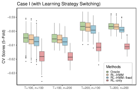
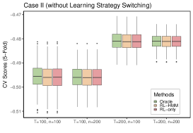
(a) Cross-validation scores	(b) Cross-validation scores
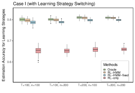
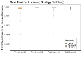
(c) Accuracy for estimating $U_{it}$	(d) Accuracy for estimating $U_{it}$

Figure 1: Boxplots show 5-fold cross-validation scores over the 200 replicates in Case I (a) and Case II (b), and boxplots show the estimation accuracy for the learning strategy over 200 replicates in Case I (c) and Case II (d). Models compared include the true model (Oracle), our proposed method (RL-HMM), RL-HMM model with time-invariant transition probabilities (RL-HMM-fixed), and the RL model without learning strategy switching (RL-only). The results for RL-HMM-fixed is not presented for Case II because cross-validation tends to select RL-HMM with time-invariant transition probabilities, making it equivalent to RL-HMM-fixed.

Finally, in both Case I and Case II, we presented the 5-fold cross-validation (CV) scores for the 200 replicates using boxplots in Figure 1 (a) and (b). The oracle (i.e., parameters are known) is compared with the RL-HMM, RL-HMM-fixed, and the RL model. In Figure 1 (a) for Case I, we observed that the RL-HMM demonstrates nearly the same performance as the oracle and outperforms RL-HMM-fixed, with RL showing the least favorable CV performance. In Figure 1 (b) for Case II, all models exhibit similar CV performance. On the other hand, recalling the estimated posterior probability of subject $i$ being in the ‘engaged’ learning strategy at trial $t$ as $\widehat{\gamma}_{i1t}=P\left(U_{it}=1\mid\mathbf{A}_{i},\widehat{\bm{\theta}}\right)$, we estimate the learning strategy at trial $t$ for subject $i$ by $\widehat{U}_{it}=I(\widehat{\gamma}_{i1t}\geq 0.5)$. We present the averaged accuracy for estimating $U_{it}$ (i.e., $(nT)^{-1}\sum_{i=1}^{n}\sum_{t=1}^{T}I(\widehat{U}_{it}=U_{it})$) for the 200 replicates using boxplots in Figure 1 (c) and (d). In Figure 1 (c) for Case I, the RL-HMM outperforms RL-HMM-fixed, with RL showing the lowest accuracy because the RL model classifies every $U_{it}$ as ‘engaged’. In Figure 1 (d) for Case II, RL-HMM estimates more than $99.9\%$ of $U_{it}$ correctly for most of the replicates, demonstrating the robustness of RL-HMM when the model is misspecified.

4 Application to EMBARC Study

4.1 Probabilistic reward task and EMBARC study

In the EMBARC study (Trivedi et al., 2016), the PRT, as introduced by Pizzagalli et al. (2005), is a computer-based experiment used to assess subjects’ ability to adapt their behavior in response to rewards. During each trial of the task, participants are presented with a cartoon face displaying one of the two stimuli (i.e., a face with a short mouth or with a long mouth). The objective for participants is to identify the type of stimulus in each trial. Crucially, the PRT provides a higher frequency of rewarding participants for correctly identifying faces with a short mouth, designating it as the ‘rich reward’, while providing less frequent rewards for correctly identifying faces with a long mouth, referred to as the ‘lean reward’. Participants receive verbal instructions outlining the task’s goal, which is to maximize the total rewards. It is essential that participants understand that not all correct responses will be rewarded. To optimize their rewards, participants should focus on providing the correct response, regardless of the face associated with the higher reward. However, the difference in mouth length between the short and long mouths is intentionally kept small. The subtle difference in mouth length often leads to difficulties in accurately perceiving the stimuli presented, resulting in a tendency to prioritize states with higher rewards over those that are more accurate.

In the EMBARC study, each PRT session comprised 200 trials, divided into two blocks of 100 trials, with a 30-second break separating the blocks. In each block, 40 correct trials were followed by reward feedback. Correct identification of the rich stimulus was associated with significantly more positive feedback (30 out of 40 trials) compared to correct identification of the lean stimulus (10 out of 40 trials). The EMBARC study was designed to discern differences in reward learning abilities between patients diagnosed with Major Depressive Disorder (MDD) and a healthy control group. The PRT experiments involved 40 subjects from the control group and 168 subjects from the MDD group. Each subject in the MDD group had two PRT sessions, one session at the baseline before treatment (week 0) and one session after one week of treatment (week 1). Subjects in the control group also took two sessions in week 0 and week 1 (no treatment at both times). More details about the EMBARC study and the PRT experiment can be found in Guo et al. (2023).

4.2 Model fitting and results

We now apply the proposed methodology to our motivating PRT data. Let $\mathcal{S}=\{0,1\}$, where $0$ and $1$ represent the type of stimulus (rich versus lean); $\mathcal{A}=\{0,1\}$, where $0$ and $1$ represent the subject choosing lean and rich stimulus, respectively. We choose the basis $\phi(a,s)=(\delta_{00},\delta_{10},\delta_{01},\delta_{11})^{\top}$, where $\delta_{uv}=I(a=u,s=v)$ $u,v\in\{0,1\}$. We assume no initial preference for one stimulus state over the other at the beginning of each session. To ensure this, we specify the initial coefficients as $\bm{\alpha}=(\alpha,0,0,\alpha)$ and set the RL intercept values as $\nu_{0}=\nu_{1}=0$. In a preliminary analysis, we observed that the learning patterns may change between the first and second block. To mitigate any potential bias, we analyze the PRT data from the first block in this paper. We started by fitting a separate RL model for each session, using the method outlined in Section 2.1, and excluded sessions with a learning rate less than $10^{-3}$. We fitted our models for the MDD group that contains subjects diagnosed with MDD at week 0 (pre-treatment) and the control group with two repeated measurements, respectively. Based on the $5$-fold cross-validation likelihood score, we choose an RL-HMM with fixed transition probabilities over trials. This model has a higher score than an RL-HMM with time-varying transition probabilities or an RL-only model without learning strategy switching. The values of $C_{01}$ are $2.8\%$ for the MDD group and $1.3\%$ for the control group. Similarly, the values of $C_{11}$ are $99.2\%$ for the MDD group and $99.7\%$ for the control group. For inference, a nonparametric bootstrap was applied to generate 200 resampling sets for each group. Bootstrap standard errors and $95\%$ bootstrap confidence intervals are shown in Table 3.

Table 3 reveals that the differences in the learning rate ($\beta$), reward sensitivity ($\rho$), and the initial probability of being in the ‘engaged’ learning strategy ($\pi_{1}$) between the MDD group and the control group are not statistically significant. This finding contrasts with previous research, such as Huys et al. (2013) and Guo et al. (2023), in which they reported a significantly lower reward sensitivity in the MDD group compared to the healthy control group in RL-only models. On the other hand, the MDD group presents a significantly lower initial coefficient ($\alpha$) compared to the control group. This indicates that the MDD group has a lower probability of selecting the correct state (i.e., distinguishing between long and short mouths) at the beginning of the task.

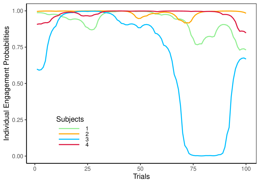
(a) Individual engagement probabilities

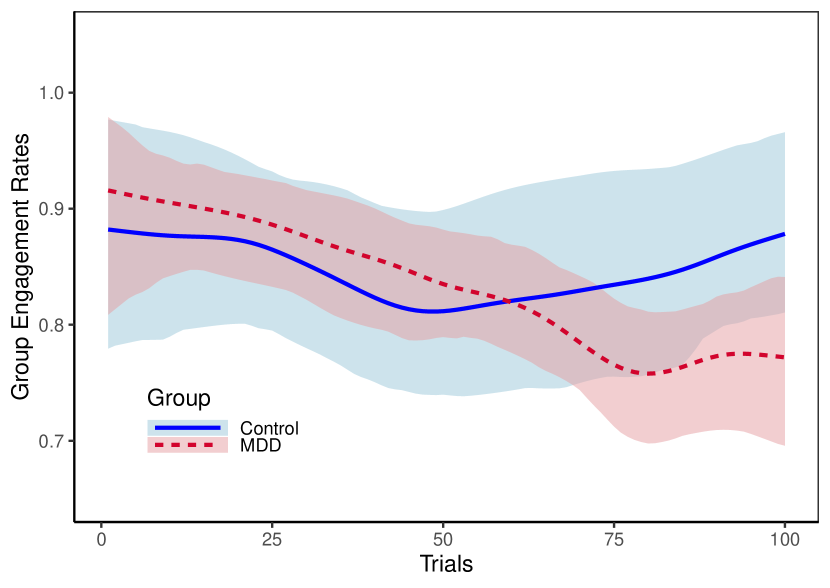
(b) Group engagement rates

Figure 2: Estimation of individual engagement probabilities (four randomly selected MDD patients) and MDD/control group engagement rates.

Recall that the posterior probability of the subject $i$ being in the ‘engaged’ learning strategy at trial $t$ is denoted as ${\gamma}_{i1}(t):={\gamma}_{i1t}=P\left(U_{it}=1\mid\mathbf{A}_{i},\bm{\theta}\right)$. We refer to this quantity as the individual engagement probability at trial $t$. Figure 2(a) presents the maximum likelihood estimates of ${\gamma}_{i1}(t)$ for four randomly selected MDD patients which shows a general decreasing tendency of being engaged but with heterogeneous patterns between patients. We define the group engagement rate at trial $t$ as the average of the individual engagement probabilities in the group (i.e. $n^{-1}\sum_{i=1}^{n}{\gamma}_{i1}(t)$). The maximum likelihood estimates and the $95\%$ pointwise bootstrap confidence intervals for the MDD and control groups engagement rates are shown in Figure 2(b). We observe that the engagement rates for MDD and control groups are similar in the first 3/4 of the task. However, the MDD group engagement rate decreases and becomes smaller in the last 1/4 of the task compared to the control group engagement rate. This implies that individuals in the MDD group are more likely to be in the ‘lapse’ state after many trials in contrast to the control group. This finding suggests an alternative explanation for the reward processing abnormalities in MDD; it may be attributed to a reduced duration of making decisions using RL rather than a diminished sensitivity to rewards.

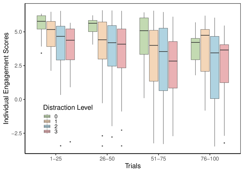
(a) Individual engagement scores

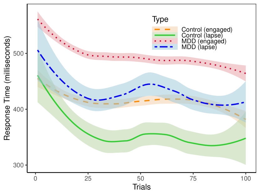
(b) Response time (ITIs)

Figure 3: Comparison of individual engagement scores versus distraction levels, and variation in response time (ITIs) across learning strategies and groups.

We define the individual engagement score as $\mbox{ES}_{i}(\mathcal{T})=\frac{1}{|\mathcal{T}|}\sum_{t\in\mathcal{T}}\log(\gamma_{i1t}/(1-\gamma_{i1t}))$. This score quantifies the average (logit transformation of) individual engagement probabilities over trials in the trial set $\mathcal{T}$. To demonstrate the utilities of engagement scores, we consider its association with a commonly used clinical measure of depression severity, the Hamilton Depression Rating Scale (HDRS) (Hamilton, 1960). In EMBARC, the HDRS was administered by trained clinicians to assess depression symptoms in different domains at the same time when the PRT was collected. One of items in HDRS assesses concentration (referred to as distraction level) on a liker scale of zero to three, where a higher value indicates greater difficulty in concentrating. In Figure 3(a), we present boxplots of individual engagement scores at different distraction levels (ranging from 0 to 3) in four periods of the task for patients in the MDD group. We observe that as the distraction level increases, the individual engagement score decreases. This effect is more pronounced in the first 3/4 of the trials. Furthermore, we performed a regression analysis of distraction levels on the individual engagement score using generalized linear models with binomial link functions. We found that the $p$-values for the coefficients are $0.004$, $0.043$, $0.013$, and $0.090$ for the four periods of the tasks, respectively. This implies that a lack of engagement, particularly at the beginning of the task, is associated with difficulties in concentration.

Define $\widehat{U}_{it}=I(\widehat{\gamma}_{i1t}\geq 0.5)$ to be the predicted type of learning strategy for the subject $i$ at trial $t$. The correct response rates (i.e. the accurate identification of short and long mouth stimuli) are $80.9\%$ and $48.4\%$ for the ‘engaged’ and ‘lapse’ state within the MDD group, and $84.3\%$ and $55.3\%$ for the control group. This suggests that the MDD group has a lower correct response rate in the ‘engaged’ state, and the correct response rate in the ‘lapse’ state is close to random guessing in both groups. Additionally, Iigaya et al. (2018) showed that different learning strategies may result in different lengths of intertrial intervals (ITIs), which is the response time between the presence of a stimulus and the decision making in a trial. Furthermore, we obtain the smoothed ITIs over trials for the two learning strategies for two groups separately using local polynomial regression (loess function in R). The mean estimates and their $95\%$ confidence intervals for the mean curves are displayed in Figure 3(b). It reveals that, on average, the ‘engaged’ learning strategy requires more time for individuals to make decisions compared to the ‘lapse’ learning strategy. Meanwhile, the control group, on average, takes less time to make decisions than the MDD group.

4.3 Brain-behavior Association

We examine whether abnormalities in reward processing may reflect underlying changes in the brain circuits that regulate reward-related behavior and learning. Specifically, we investigate whether dysfunctions in MDD-implicated brain circuitries affect learning abilities by an association analysis of subjects’ individual engagement scores and task functional magnetic resonance imaging (fMRI) measures of brain activation. We focus on fMRI measures in an emotional conflict task assessing amygdala-anterior cingulate (ACC) circuitry (Etkin et al., 2006; Fonzo et al., 2019). The emotional conflict task comprises four types of trials: congruent (C) trials, incongruent (I) trials, incongruent followed by incongruent (iI) trials, and incongruent followed by congruent (cI) trials.

To investigate the brain-behavior association for each brain region of interest (ROI), the voxel-level activation conflicts (I-C) and activation conflict adaptations (iI - cI) within each ROI for each subject in the MDD group before treatment were computed. To investigate interregional interaction between ROIs, a psychophysiological interaction (PPI) analysis, as outlined in Etkin et al. (2006), provides voxel-wise conflict adaptation coupling between two ROIs. As a result, we considered six types of fMRI measures: (i) mean of activation conflicts within ROIs (I-C mean), (ii) mean of activation conflict adaptations within ROIs (iI-cI mean), (iii) mean of conflict adaptation coupling between two ROIs (PPI mean), (iv) standard deviation of activation conflicts within ROIs (I-C std), (v) standard deviation of activation conflict adaptations within ROIs (iI-cI std), and (vi) standard deviation of conflict adaptation coupling between two ROIs (PPI std). We utilize linear regressions to model the associations between individual engagement scores and each fMRI measure for all ROIs/interactions. Subsequently, we calculate the p-values for the regression coefficients and implement q-values for controlling the false discovery rate (FDR), as proposed by (Benjamini and Hochberg, 1995).

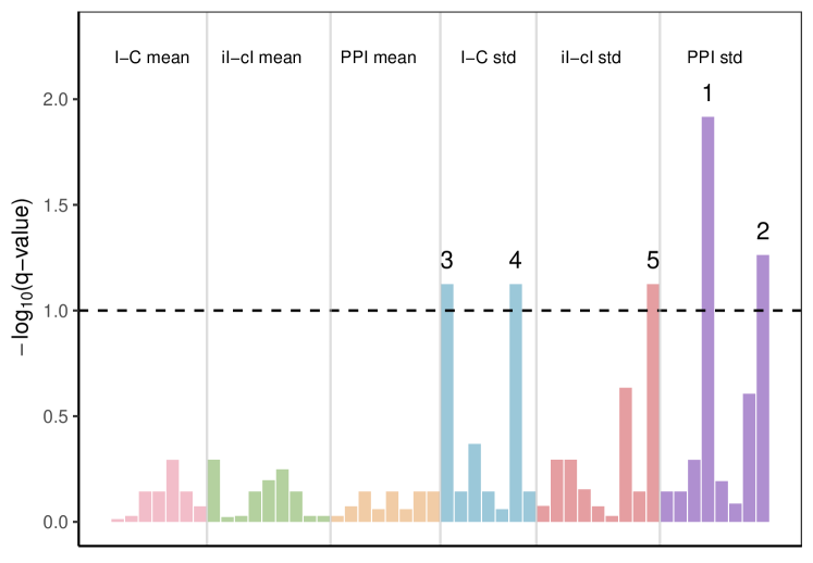
(a) $-\log_{10}(\text{q-value})$ of the brain-behavior association

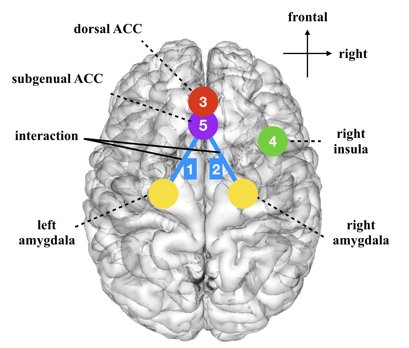
(b) ROIs and ROI interactions identified

Figure 4: (a): The ($-\log_{10}$ transformation of) q-values of the regression coefficients for individual engagement scores regressed on each fMRI measure across all ROIs/interactions. The dashed line indicates the FDR at $10\%$. (b): Visualization of significant ROIs/interactions in the brain, with each number (1 to 5) corresponding to the respective q-value in (a).

The results are depicted in Figure 4. In Figure 4(a), each $q$-value undergoes a transformation using a negative $\log_{10}$ function, with the dashed line representing the FDR at $10\%$. Three ROIs and two ROI interactions were detected. A visualization illustrating the detected ROIs or interactions in the brain is presented in Figure 4(b), where the associations between engagement scores and the brain response to emotional conflict adaptation coupling of subgenual ACC ROI and left amygdala ROI appears to be the most significant. Other significant associations include the conflict coupling of subgenual ACC and right amygdala, the conflict within dorsal ACC and right insula, and the conflict adaptations within the subgenual ACC. In this analysis, all significant brain measures identified were the standard deviations of ROIs, rather than their mean effects. In addition, our results show a negative correlation between engagement scores and the standard deviations of all five identified ROIs or interactions. This suggests that an increased engagement in reward learning tasks corresponds to a decreased variability in brain activity during an emotional conflict task. Williams (2016) further indicated that the ACC—amygdala connectivity belongs to the negative affect circuit. Hence, MDD patients are more prone to lose concentration during the reward learning behavioral task, which could be due to an increase of fluctuation (or instability) of brain activities within the negative affect circuit.

5 Discussion

In this paper, we propose a RL-HMM method to characterize reward-based decision-making, incorporating the switching of learning strategies between two states: the ‘engaged’ state, where subjects make decisions based on the RL model, and the ‘lapse’ state, where they make random choices. We extend the RL model to accommodate a non-discrete state space and posit time-varying transition probabilities within the HMM. For parameter estimation, we employ the EM algorithm. In the E-step, we apply forward-backward inductive computation, and in the M-step, we implement a computationally efficient algorithm for one-step updates of all the parameters. Extensive simulation studies validate the finite-sample performance of our method.

Applying our approach to the EMBARC, we discovered different phenomena from the findings in Huys et al. (2013) and Guo et al. (2023), where the MDD group had a lower reward sensitivity compared to the healthy controls. In contrast, our method did not identify a significant group difference in reward sensitivity. Instead, we discovered that the MDD group spent a larger proportion of time using the ‘lapse’ strategy compared to the healthy group. This suggests an alternative mechanism of the reward processing abnormalities in MDD. We identified a significant correlation between the individual engagement score and a clinician-assessed measure of concentration difficulty. This finding suggests that tendencies towards disengagement may be linked with a loss of concentration ability in MDD. Moreover, our analysis revealed that the ‘lapse’ strategy requires less time for individuals to respond than the ‘engaged’ strategy in PRT. Using additional brain fMRI data within the same study, we found that the individual engagement scores computed from RL-HMM are associated with the variability of brain activities in the negative affect circuitry under an emotional conflict task (Etkin et al., 2006). This brain-behavior association study suggests that a higher heterogeneity in brain activities during emotional conflict is associated with lower engagement in reward learning tasks.

Our methods are sufficiently general to analyze other types of behavioral tasks. Some extensions include to introduce covariates to model between-subjects heterogeneity in learning processes and jointly model PRT with other phenotypes including brain measures and clinical outcomes.

Table 1: Summary of the parameter estimates in 200 simulations for Case I (data generated from RL-HMM).

			RL-HMM					RL-HMM-fixed			RL-only
$T$	$n$	Parameters	Bias	SD	SE	CP		Bias	SD		Bias	SD
100	100	$\beta$	-0.0005	0.0073	0.0076	93		-0.0067	0.0070		-0.0070	0.0166
		$\rho$	0.1004	0.3741	0.3664	94		0.0775	0.3674		-1.7117	0.3954
		$\nu_{1}$	-0.0073	0.0790	0.0755	93		-0.0357	0.0708		-0.0003	0.0539
		$\alpha$	0.0182	0.1133	0.1211	98		-0.1577	0.1085		-0.9368	0.0571
		$\pi_{1}$	-0.0148	0.1346	0.1269	94		-0.0460	0.1030
		$\zeta_{0}(T/4)$	-0.1326	0.2693	0.2908	93		-1.0037	0.1787
		$\zeta_{0}(3T/4)$	0.1054	0.2575	0.2966	97		0.4963	0.1787		————
		$\zeta_{1}(T/4)$	0.1111	0.2583	0.2816	96		1.2878	0.2042
		$\zeta_{1}(3T/4)$	-0.1410	0.2731	0.3158	94		-0.7122	0.2042
100	200	$\beta$	-0.0001	0.0054	0.0053	94		-0.0066	0.0051		-0.0079	0.0123
		$\rho$	0.0685	0.2594	0.2542	93		0.0627	0.2590		-1.7494	0.2923
		$\nu_{1}$	-0.0023	0.0513	0.0527	97		-0.0303	0.0468		-0.0007	0.0354
		$\alpha$	0.0172	0.0832	0.0848	96		-0.1494	0.0830		-0.9404	0.0395
		$\pi_{1}$	-0.0008	0.0942	0.0916	95		-0.0357	0.0798
		$\zeta_{0}(T/4)$	-0.1182	0.2044	0.2133	93		-1.0036	0.1288
		$\zeta_{0}(3T/4)$	0.1022	0.1878	0.2013	96		0.4964	0.1288		————
		$\zeta_{1}(T/4)$	0.0896	0.1966	0.2079	92		1.2645	0.1697
		$\zeta_{1}(3T/4)$	-0.1301	0.2134	0.2252	93		-0.7355	0.1697
200	100	$\beta$	0.0000	0.0049	0.0050	93		-0.0057	0.0047		-0.0015	0.0108
		$\rho$	0.0729	0.2747	0.2661	93		0.0584	0.2647		-2.0046	0.2450
		$\nu_{1}$	-0.0087	0.0655	0.0608	94		-0.0561	0.0589		0.0230	0.0480
		$\alpha$	0.0071	0.0948	0.0903	95		-0.1587	0.0906		-0.9270	0.0469
		$\pi_{1}$	-0.0107	0.1333	0.1221	94		-0.0377	0.1182
		$\zeta_{0}(T/4)$	-0.0936	0.1840	0.1982	93		-0.9678	0.1298
		$\zeta_{0}(3T/4)$	0.1125	0.1898	0.1974	91		0.5322	0.1298		————
		$\zeta_{1}(T/4)$	0.1035	0.1706	0.1935	94		1.2598	0.1505
		$\zeta_{1}(3T/4)$	-0.1158	0.1854	0.2038	93		-0.7402	0.1505
200	200	$\beta$	-0.0004	0.0035	0.0035	95		-0.0062	0.0033		-0.0013	0.0074
		$\rho$	0.0532	0.1790	0.1863	94		0.0511	0.1747		-2.0268	0.1701
		$\nu_{1}$	-0.0076	0.0434	0.0434	95		-0.0548	0.0402		0.0263	0.0339
		$\alpha$	0.0046	0.0641	0.0631	95		-0.1543	0.0594		-0.9235	0.0347
		$\pi_{1}$	0.0015	0.0913	0.0887	97		-0.0376	0.0753
		$\zeta_{0}(T/4)$	-0.0625	0.1447	0.1484	96		-0.9533	0.0805
		$\zeta_{0}(3T/4)$	0.0652	0.1236	0.1424	95		0.5467	0.0805		————
		$\zeta_{1}(T/4)$	0.0669	0.1366	0.1427	94		1.2436	0.0940
		$\zeta_{1}(3T/4)$	-0.0793	0.1352	0.1447	93		-0.7564	0.0940

(Bias): estimate bias; (SD): standard deviation; (SE): average bootstrap standard error; (CP): coverage probability of the $95\%$ bootstrap confidence intervals; (RL-HMM): our proposed method; (RL-HMM-fixed): RL-HMM model with time-invariant transition probabilities; (RL-only): the RL model without learning strategy switching.

Table 2: Summary of the parameter estimates in 200 simulations for Case II (data generated from RL-only model).

			RL-HMM			RL-only
$T$	$n$	Parameters	Bias	SD		Bias	SD
100	100	$\beta$	0.0004	0.0047		0.0005	0.0046
		$\rho$	0.0955	0.2223		0.0053	0.2027
		$\nu_{1}$	0.0008	0.0484		0.0014	0.0473
		$\alpha$	0.0488	0.0571		0.0070	0.0466
100	200	$\beta$	-0.0002	0.0035		-0.0005	0.0046
		$\rho$	0.0920	0.1671		0.0102	0.2027
		$\nu_{1}$	-0.0009	0.0364		0.0001	0.0357
		$\alpha$	0.0393	0.0429		0.0029	0.0390
200	100	$\beta$	0.0001	0.0034		0.0002	0.0034
		$\rho$	0.0743	0.1810		-0.0011	0.1722
		$\nu_{1}$	-0.0014	0.0406		0.0002	0.0398
		$\alpha$	0.0362	0.0451		0.0039	0.0418
200	200	$\beta$	0.0000	0.0021		0.0001	0.0021
		$\rho$	0.0661	0.1207		-0.0043	0.1155
		$\nu_{1}$	0.0009	0.0269		0.0026	0.0263
		$\alpha$	0.0305	0.0318		0.0010	0.0298

(Bias): estimate bias; (SD): standard deviation; (RL-HMM): our proposed method; (RL-only): the RL model without learning strategy switching. The results for RL-HMM-fixed is not presented for Case II because cross-validation tends to select RL-HMM with time-invariant transition probabilities, making it equivalent to RL-HMM-fixed.

Table 3: Parameter estimation in EMBARC study under the proposed method for MDD group, control group, and group contrast.

	MDD				Control				MDD - Control
Pars.	Est.	Err.	$95\%$ CI		Est.	Err.	$95\%$ CI		$95\%$ CI
$\beta$	0.031	0.009	(0.012, 0.049)		0.031	0.009	(0.015, 0.048)		(-0.026, 0.025)
$\rho$	3.338	0.327	(2.696, 3.980)		3.292	0.337	(2.631, 3.953)		(-0.853, 0.945)
$\alpha$	1.328	0.072	(1.187, 1.470)		1.853	0.177	(1.506, 2.200)		(-0.893, -0.155)
$\pi_{1}$	0.917	0.042	(0.773, 0.973)		0.882	0.057	(0.659, 0.967)		(-0.985, 0.159)

References

- Arnold and Tibshirani (2016) Arnold, Taylor B and Tibshirani, Ryan J. (2016). Efficient implementations of the generalized lasso dual path algorithm. Journal of Computational and Graphical Statistics 25(1), 1–27.
- Ashwood et al. (2022) Ashwood, Zoe C, Roy, Nicholas A, Stone, Iris R, Urai, Anne E, Churchland, Anne K, Pouget, Alexandre and Pillow, Jonathan W. (2022). Mice alternate between discrete strategies during perceptual decision-making. Nature Neuroscience 25(2), 201–212.
- Baum et al. (1970) Baum, Leonard E, Petrie, Ted, Soules, George and Weiss, Norman. (1970). A maximization technique occurring in the statistical analysis of probabilistic functions of markov chains. The Annals of Mathematical Statistics 41(1), 164–171.
- Benjamini and Hochberg (1995) Benjamini, Yoav and Hochberg, Yosef. (1995). Controlling the false discovery rate: a practical and powerful approach to multiple testing. Journal of the Royal statistical society: series B (Methodological) 57(1), 289–300.
- Byrd et al. (1995) Byrd, Richard H, Lu, Peihuang, Nocedal, Jorge and Zhu, Ciyou. (1995). A limited memory algorithm for bound constrained optimization. SIAM Journal on Scientific Computing 16(5), 1190–1208.
- Chen et al. (2021) Chen, Cathy S, Knep, Evan, Han, Autumn, Ebitz, R Becket and Grissom, Nicola M. (2021). Sex differences in learning from exploration. Elife 10, e69748.
- Dempster et al. (1977) Dempster, Arthur P, Laird, Nan M and Rubin, Donald B. (1977). Maximum likelihood from incomplete data via the em algorithm. Journal of the Royal Statistical Society: Series B (Statistical Methodology) 39(1), 1–22.
- Etkin et al. (2006) Etkin, Amit, Egner, Tobias, Peraza, Daniel M, Kandel, Eric R and Hirsch, Joy. (2006). Resolving emotional conflict: A role for the rostral anterior cingulate cortex in modulating activity in the amygdala. Neuron 51(6), 871–882.
- Fonzo et al. (2019) Fonzo, Gregory A, Etkin, Amit, Zhang, Yu, Wu, Wei, Cooper, Crystal, Chin-Fatt, Cherise, Jha, Manish K, Trombello, Joseph, Deckersbach, Thilo, Adams, Phil et al. (2019). Brain regulation of emotional conflict predicts antidepressant treatment response for depression. Nature Human Behaviour 3(12), 1319–1331.
- Guo et al. (2023) Guo, Xingche, Zeng, Donglin and Wang, Yuanjia. (2023). A semiparametric inverse reinforcement learning approach to characterize decision making for mental disorders. Journal of the American Statistical Association (just-accepted), 1–21.
- Hamilton (1960) Hamilton, Max. (1960). A rating scale for depression. Journal of Neurology, Neurosurgery, and Psychiatry 23(1), 56.
- Huys et al. (2011) Huys, Quentin JM, Cools, Roshan, Gölzer, Martin, Friedel, Eva, Heinz, Andreas, Dolan, Raymond J and Dayan, Peter. (2011). Disentangling the roles of approach, activation and valence in instrumental and pavlovian responding. PLoS computational biology 7(4), e1002028.
- Huys et al. (2016) Huys, Quentin JM, Maia, Tiago V and Frank, Michael J. (2016). Computational psychiatry as a bridge from neuroscience to clinical applications. Nature Neuroscience 19(3), 404–413.
- Huys et al. (2013) Huys, Quentin JM, Pizzagalli, Diego A, Bogdan, Ryan and Dayan, Peter. (2013). Mapping anhedonia onto reinforcement learning: A behavioural meta-analysis. Biology of Mood & Anxiety Disorders 3(1), 1–16.
- Iigaya et al. (2018) Iigaya, Kiyohito, Fonseca, Madalena S, Murakami, Masayoshi, Mainen, Zachary F and Dayan, Peter. (2018). An effect of serotonergic stimulation on learning rates for rewards apparent after long intertrial intervals. Nature Communications 9(1), 1–10.
- Insel et al. (2010) Insel, Thomas, Cuthbert, Bruce, Garvey, Marjorie, Heinssen, Robert, Pine, Daniel S, Quinn, Kevin, Sanislow, Charles and Wang, Philip. (2010). Research domain criteria (RDoC): Toward a new classification framework for research on mental disorders. American Journal of Psychiatry 167(7), 748–751.
- Kendler et al. (1999) Kendler, Kenneth S, Karkowski, Laura M and Prescott, Carol A. (1999). Causal relationship between stressful life events and the onset of major depression. American Journal of Psychiatry 156(6), 837–841.
- Pizzagalli et al. (2005) Pizzagalli, Diego A, Jahn, Allison L and O’Shea, James P. (2005). Toward an objective characterization of an anhedonic phenotype: A signal-detection approach. Biological Psychiatry 57(4), 319–327.
- Rescorla (1972) Rescorla, Robert A. (1972). A theory of pavlovian conditioning: Variations in the effectiveness of rreinforcement and nonreinforcement. Current Research and Theory, 64–99.
- Rush et al. (2006) Rush, A John, Kraemer, Helena C, Sackeim, Harold A, Fava, Maurizio, Trivedi, Madhukar H, Frank, Ellen, Ninan, Philip T, Thase, Michael E, Gelenberg, Alan J, Kupfer, David J et al. (2006). Report by the acnp task force on response and remission in major depressive disorder. Neuropsychopharmacology 31(9), 1841–1853.
- Schultz et al. (1997) Schultz, Wolfram, Dayan, Peter and Montague, P Read. (1997). A neural substrate of prediction and reward. Science 275(5306), 1593–1599.
- Sutton and Barto (2018) Sutton, Richard S and Barto, Andrew G. (2018). Reinforcement Learning: An Introduction. MIT press.
- Tibshirani et al. (2005) Tibshirani, Robert, Saunders, Michael, Rosset, Saharon, Zhu, Ji and Knight, Keith. (2005). Sparsity and smoothness via the fused lasso. Journal of the Royal Statistical Society: Series B (Statistical Methodology) 67(1), 91–108.
- Tibshirani (2014) Tibshirani, Ryan J. (2014). Adaptive piecewise polynomial estimation via trend filtering. The Annals of Statistics 42(1), 285–323.
- Tibshirani and Taylor (2011) Tibshirani, Ryan J and Taylor, Jonathan. (2011). The solution path of the generalized lasso. Annals of Statistics 39(3), 1335–1371.
- Trivedi et al. (2016) Trivedi, Madhukar H, McGrath, Patrick J, Fava, Maurizio, Parsey, Ramin V, Kurian, Benji T, Phillips, Mary L, Oquendo, Maria A, Bruder, Gerard, Pizzagalli, Diego, Toups, Marisa et al. (2016). Establishing moderators and biosignatures of antidepressant response in clinical care (embarc): Rationale and design. Journal of Psychiatric Research 78, 11–23.
- Williams (2016) Williams, Leanne M. (2016). Precision psychiatry: A neural circuit taxonomy for depression and anxiety. The Lancet Psychiatry 3(5), 472–480.
- Worthy et al. (2013) Worthy, Darrell A, Hawthorne, Melissa J and Otto, A Ross. (2013). Heterogeneity of strategy use in the iowa gambling task: A comparison of win-stay/lose-shift and reinforcement learning models. Psychonomic Bulletin & Review 20(2), 364–371.