The Gross-Pitaevskii equation for a infinite square-well with a delta-function barrier

Abstract

The Gross-Pitaevskii equation is solved by analytic methods for an external double-well potential that is an infinite square well plus a $\delta$-function central barrier. We find solutions that have the symmetry of the non-interacting Hamiltonian as well as asymmetric solutions that bifurcate from the symmetric solutions for attractive interactions and from the antisymmetric solutions for repulsive interactions. We present a variational approximation to the asymmetric state as well as an approximate numerical approach. Stability of the states is briefly considered.

I Introduction

The properties of Bose-Einstein condensates in a double-well potential [1]-[14] have received considerable attention in recent years. The solution of the Gross-Pitaevskii equation (GPE) with an external double well shows some interesting nonlinear effects, in particular bifurcations to symmetry-breaking states in both atomic [3]-[18] and optical systems [19]-[22] and unusual dynamics, e.g., self-trapping [1, 4, 5, 7, 8]. Symmetry breaking has been observed experimentally in several types of systems [19, 21, 22, 23]. In a simple infinite square well, the equation has exact analytic solutions in terms of Jacobi elliptical functions [24, 25]. When we add a repulsive Dirac $\delta$-function at the center of the well, we get a double well that also is soluble exactly. We call this the box-$\delta$ potential. We can find exact analytic results for the asymmetric solutions as well.

The time dependent GPE is

$$i\hbar\frac{\partial\Phi}{\partial t}=\left(-\frac{\hbar^{2}}{2\bar{m}}\frac{\partial^{2}}{\partial z^{2}}+V_{ex}(z)+g\left|\Phi\right|^{2}\right)\Phi$$ (1)

with $\Phi$ normalized to $N$; $\bar{m}$ is the particle mass. Our infinite well potential goes from position $z=-a$ to $a.$ Let $x=z/a$ and energy be measured in units of $\hbar^{2}/2\bar{m}a^{2}.$ We assume an exponential time dependence for the wave function, $\Phi(x,t)=e^{i\mu t}\psi(x),$ so the unitless time-independent GPE for the box-delta potential can be written in the form

$$\left[-\frac{d^{2}}{dx^{2}}+V(x)+\eta N\left|\psi(x)\right|^{2}\right]\psi(x)=\mu\psi(x),$$ (2)

with $\int dx\left|\psi(x)\right|^{2}=1$, $\eta=2\bar{m}a^{2}g/\hbar^{2}$ and

$$V(x)=\left\{\begin{array}[]{cc}\infty,&\left|x\right|\geq 1\\ \gamma\delta(x),&\left|x\right|<1\end{array}\right..$$ (3)

A potential somewhat similar to what we consider here was a $\delta$-function within a harmonic potential [10]. Refs. [17] - [18] treat the GPE in the box-$\delta$ potential numerically (using a narrow Gaussian to simulate the $\delta$-function), with approximations valid for large $\gamma$ and small $\gamma$, and by a variational approach. We treat it exactly and will compare with results given in these references.

II Repulsive interactions

Here we treat the states that preserve the symmetry of the non-interacting Hamiltonian; asymmetric states are treated later. Some details of the Jacobi elliptic functions are given in the Appendix.

II.1 Antisymmetric states

These states do not see the $\delta$-function and so are equivalent to the antisymmetric states of the pure square well [24]. Substitute the function

$$\psi(x)=A\mathrm{sn}\left(kx|m\right),$$ (4)

where $\mathrm{sn}$ is the elliptic sine, into Eq. (2) and equate the coefficients of different powers of $\mathrm{sn}$ to zero to give

$$A^{2} = \frac{2k^{2}m}{\eta N},$$ (5)

$$\mu = k^{2}\left(1+m\right).$$ (6)

Here we see that we are dealing with a repulsive interaction $\eta>0$ because $A^{2}$ is positive. The solution has $\mathrm{sn}\left(0|m\right)=0$, as it must be for the antisymmetric functions. The boundary conditions at $x=\pm 1$ are satisfied with

$$k=2jK(m),$$ (7)

with $j=1,2\ldots$ and $K(m)$ is the elliptical integral of the first kind (see Appendix Eq. (78)). The normalization integral is

$$A^{2}\int_{-1}^{1}dx\left(\mathrm{sn}(2jK(m)x|m\right)^{2}=\frac{2A^{2}}{K(m)m}\left[-E(m)+K(m)\right]=1,$$ (8)

where $E(m)$ is the complete elliptic integral of the second kind (see Appendix Eq. (80)). (This normalization integral is independent of integer $j.$) The combination of Eqs. (5) and (8) determine the variable $m,$ which in turn gives the eigenvalue $\mu$ by Eq. (6). We must solve

$$\frac{16j^{2}K(m)}{\eta N}\left[-E(m)+K(m)\right]=1$$ (9)

to find $m$. For example, for $j=1$ and $\eta N=10$ we find $m=0.379$ and $\mu=17.16$; for $j=2$, $m=0.1172$ and $\mu=46.92$. Fig. 1 shows an example of this state.

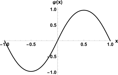
Figure 1: The lowest antisymmetric state of the box-delta well GPE with $\eta N=10$. The state does not see the $\delta$-function.

II.2 Symmetric states

The symmetric wave function that satisfies the boundary conditions is

$$\psi(x)=\left\{\begin{array}[]{cc}A\mathrm{sn(}k(x+1)|m),&-1<x<0\\ -A\mathrm{sn}(k(x-1)|m),&0\leq x<1\end{array}\right..$$ (10)

This solution satisfies the GPE with the same conditions of Eqs. (5) and (6). The condition on the wave function derivatives at $x=0$ is

$$\Delta\psi^{\prime}(0)=\lim_{\varepsilon\rightarrow 0}(\psi^{\prime}(\varepsilon)-\psi^{\prime}(-\varepsilon))=\gamma\psi(0),$$

which becomes here

$$2k\mathrm{cn(k|m)\mathrm{dn(k|m)+\gamma\mathrm{sn}(k|m)=0}.}$$ (11)

The normalization becomes

$$A^{2}\frac{2(k-\mathcal{E}(k|m))}{km}=1,$$ (12)

where $\mathcal{E}(k|m)$ is the Jacobi Epsilon function (see Appendix Eq. (81)). Given the condition of Eq. (5) we must solve

$$\frac{4k}{\eta N}(k-\mathcal{E}(k|m))-1=0$$ (13)

simultaneously with that of Eq. (11) for $k$ and $m.$

For $\gamma=10$ and $\eta N=10,$ we find the solutions for the lowest energies as

$$k = 3.067;\quad m=0.433;\quad\mu=13.48,$$ (14)

$$k = 5.680;\quad m=0.140;\quad\mu=36.77.$$ (15)

Plots of these are shown in Fig. 2.

      

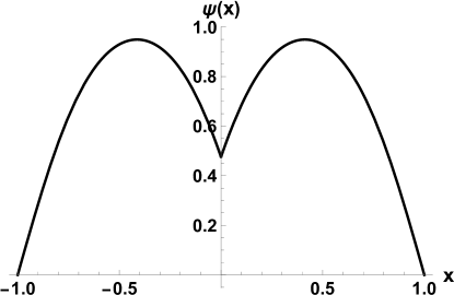
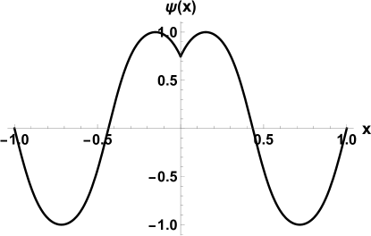
Figure 2: The lowest two symmetric states of the box-delta well GPE with $\gamma=10$ and $\eta N=10.$

III Attractive interactions

Here we again consider the states that maintain the symmetry of the non-interacting Hamiltonian.

III.1 Antisymmetric states

As in Sec. II.1, the states are the same as those where there is no $\delta$-function, which were treated in Ref. [25]. The wave function

$$\psi(x)=A\mathrm{cn}(kx+\delta|m),$$ (16)

where $\mathrm{cn}(x|m)$ is the elliptic cosine, satisfies the GPE with

$$A^{2}=-\frac{2mk^{2}}{\eta N},$$ (17)

with $\eta N$ negative for attraction. The other condition is

$$\mu=k^{2}(1-2m).$$ (18)

The antisymmetric states have

$$\delta = -K(m),$$ (19)

$$k = 2jK(m),$$ (20)

where $j=1,2,\ldots$ . The normalization equation combined with Eq. (17) gives the condition

$$2\left[\frac{2\left(2jK(m)\right)^{2}}{\left|\eta N\right|}\right]\frac{E[m]+(m-1)K[m]}{K[m]}=1$$ (21)

to determine $m$.

III.2 Symmetric states

The symmetric states are given by

$$\psi(x)=\left\{\begin{array}[]{cc}A\mathrm{cn(}k(x+1)-K(m)|m),&-1<x<0\\ -A\mathrm{cn}(k(x-1)-K(m)|m),&0\leq x<1\end{array}\right.$$ (22)

with again the conditions of Eqs. (17) and (18) applying to $A$ and $\mu$ in order to satisfy the GPE. The derivative condition at $x=0$ gives

$$2k\mathrm{sn(}k+K(m)|m)\mathrm{dn(}k+K(m)|m)=\gamma\mathrm{cn(}k+K(m)|m).$$ (23)

The normalization condition is

$$\frac{2A^{2}}{km\mathrm{dn}(k|m)}\left[k(m-1)\mathrm{dn}(k|m)+\mathrm{dn}(k|m)\mathcal{E}(k|m)-m\mathrm{cn}(k|m)\mathrm{sn}(k|m)\right]=1.$$ (24)

Thus we must solve Eq. (23) and the following simultaneously to find $k$ and $m$:

$$\frac{4k}{\left|\eta N\right|\mathrm{dn}(k|m)}\left[k(m-1)\mathrm{dn}(k|m)+\mathrm{dn}(k|m)\mathcal{E}(k|m)-m\mathrm{cn}(k|m)\mathrm{sn}(k|m)\right]=1.$$ (25)

For $\gamma=10,\eta N=-10,$ we find the lowest two state roots at $\{k,m\}=\{3.085,0.490\}$ and $\{5.651,0.146\}$ corresponding to chemical potentials of 0.187 and 22.602, respectively. A wave function here looks similar to that in the repulsive analysis, except that the amplitude is larger at the peaks and smaller at the $\delta$-function.

IV Asymmetric solutions

The GPE is nonlinear and so has the possibility of developing asymmetric solutions. The Hamiltonian includes the wave function and so becomes asymmetric itself when the wave function does. Thus the usual proof of symmetry or antisymmetry breaks down.

IV.1 Attractive interactions

For an attractive interaction, the general wave function that satisfies the boundary conditions at $x=\pm 1$, but is not necessarily symmetric or antisymmetric is

$$\psi(x)=\left\{\begin{array}[]{cc}A_{1}\mathrm{cn(}k_{1}(x+1)-K(m_{1})|m_{1}),&-1<x<0\\ A_{2}\mathrm{cn}(k_{2}(x-1)-K(m_{2})|m_{2}),&0\leq x<1\end{array}\right..$$ (26)

There are six variables to be determined here. The amplitudes and chemical potentials, as in Sec. III.1, obey

$$A_{i}^{2} = -\frac{2m_{i}k_{i}^{2}}{\eta N},$$ (27)

$$\mu_{i} = k_{i}^{2}(1-2m_{i}).$$ (28)

The wave function must be continuous at $x=0$ giving

$$A_{1}\mathrm{cn(}k_{1}-K(m_{1})|m_{1})=A_{2}\mathrm{cn}(k_{2}+K(m_{2})|m_{2}).$$ (29)

The chemical potentials must be uniform over the whole system so that we have

$$k_{1}^{2}(1-2m_{1})=k_{2}^{2}(1-2m_{2}).$$ (30)

If we integrate in order to satisfy the normalization then we find

$$\frac{A_{1}^{2}}{k_{1}m_{1}\mathrm{dn}(k_{1}|m_{1})}\left[\left(k_{1}(m_{1}-1)+\mathcal{E}(k_{1}|m_{1})\right)\mathrm{dn}(k_{1}|m_{1})-m_{1}\mathrm{cn}(k_{1}|m_{1})\mathrm{sn}(k_{1}|m_{1})\right]+$$

$$+\frac{A_{2}^{2}}{k_{2}m_{2}\mathrm{dn}(k_{2}|m_{2})}\left[\left(k_{2}(m_{2}-1)+\mathcal{E}(k_{2}|m_{2})\right)\mathrm{dn}(k_{2}|m_{2})-m_{2}\mathrm{cn}(k_{2}|m_{2})\mathrm{sn}(k_{2}|m_{2})\right] = 1.$$ (31)

The wave function derivative difference at $x=0$ obeys the condition

$$-A_{2}k_{2}\mathrm{sn}(-k_{2}-K(m_{2})|m_{2})\mathrm{dn}(-k_{2}-K(m_{2})|m_{2})+$$

$$+A_{1}k_{1}\mathrm{sn}(k_{1}-K(m_{1})|m_{1})\mathrm{dn}(k_{1}-K(m_{1})|m_{1}) = \gamma A_{1}\mathrm{cn}(k_{1}-K(m_{1})|m_{1}).$$ (32)

These six conditions must be solved simultaneously for $A_{i}$, $k_{i}$, and $m_{i}$, which can be done, for example, by use of $\mathit{Mathematica^{\prime}s}$ FindRoot command. A ground state and an excited state are shown in Fig. 3.

      

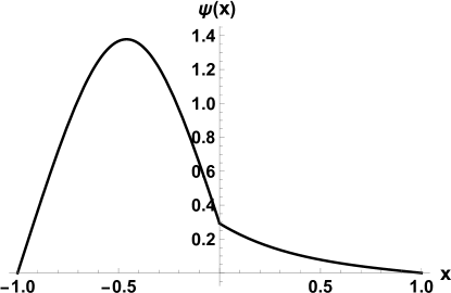
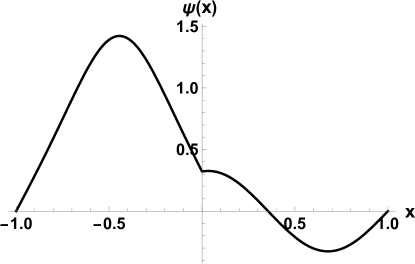
Figure 3: Exact analytic asymmetric states of the box-$\delta$ potential GPE for attractive interactions. (Left) A zero node state for $\gamma=10$ and $\eta N=-2.73.$ (Right) A one-node state corresponding to $\gamma=10$ and $\eta N=-10.2.$ Solutions that are mirror images of these are degenerate.

Note that the main peak in each of these is in the left side; there are clearly degenerate mirror-image states with the main peak in the right well. As we will see below these states bifurcate from the symmetric states at appropriate interaction parameter values.

IV.2 Repulsive interactions

For a repulsive interaction, the general wave function that satisfies the boundary conditions at $x=\pm 1$, but is not necessarily symmetric or antisymmetric is

$$\psi(x)=\left\{\begin{array}[]{cc}A_{1}\mathrm{sn(}k_{1}(x+1)|m_{1}),&-1<x<0\\ A_{2}\mathrm{sn}(k_{2}(x-1)|m_{2}),&0\leq x<1.\end{array}\right.$$ (33)

There are again six variables to be determined. The amplitudes and chemical potentials, as in Sec.II.1 obey

$$A_{i}^{2} = \frac{2m_{i}k_{i}^{2}}{\eta N},$$ (34)

$$\mu_{i} = k_{i}^{2}(1+m_{i}).$$ (35)

We use Eqs. (34) as the first two conditions. Then Eq. (35) gives us the condition

$$k_{1}^{2}(1+m_{1})=k_{2}^{2}(1+m_{2}).$$ (36)

Continuity of the function at $x=0$ implies

$$A_{1}\mathrm{sn(}k_{1}|m_{1})=A_{2}\mathrm{sn(}-k_{2}|m_{2}).$$ (37)

The derivative condition on the wave function due to the $\delta$-function is

$$A_{2}k_{2}\mathrm{cn}(-k_{2}|m_{2})\mathrm{dn}(-k_{2}|m_{2})-A_{1}k_{1}\mathrm{cn}(k_{1}|m_{1})\mathrm{dn}(k_{1}|m_{1})=\gamma A_{1}\mathrm{sn}(k_{1}|m_{1}).$$ (38)

The last condition is the normalization, which is

$$\frac{\left[A_{2}^{2}k_{1}k_{2}m_{1}+A_{1}^{2}k_{1}k_{2}m_{2}-A_{1}^{2}k_{2}m_{2}\mathcal{E}(k_{1}|m_{1})-A_{2}^{2}k_{1}m_{1}\mathcal{E}(k_{2}|m_{2})\right]}{k_{1}k_{2}m_{1}m_{2}}=1.$$ (39)

These states bifurcate from the repulsive antisymmetric states. As we try a sequence of $\eta N$ values with $\eta N$ decreasing, the states that are generated finally evolve from asymmetric into the antisymmetric states at the bifurcation value. We show a typical repulsive state in Fig. 4.

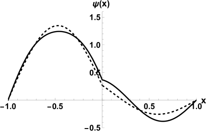
Figure 4: (Solid) An asymmetric state solving the GPE for $\gamma=10$ and a repulsive interaction of $\eta N=10$. (Dashed) The variational state at the same parameters. Because the state arises from a bifurcation from antisymmetric states it has one node.

In Fig. 5 we summarize the exact results by showing the attractive and repulsive symmetric, antisymmetric and asymmetric energies per particle all on one graph.

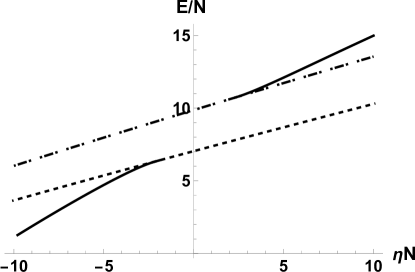
Figure 5: Exact energies for the states: (Dashed) symmetric; (dot-dashed) antisymmetric; (Solid) asymmetric, both attractive and repulsive. The critical attractive bifurcation point of the symmetric state with the asymmetric state is at $\eta_{c}N=-2.07$. For repulsive interaction parameters the bifurcation point for the asymmetric state energy and the antisymmetric state is $\eta_{c}N=2.34$. In all cases $\gamma=10.$

IV.3 Two-mode approximation for asymmetric states

We use an approximation method given in Refs. [10, 11] for a different potential. The unitless time-dependent GPE is

$$i\frac{\partial\psi}{\partial t}=\left[H_{0}+\eta N\left|\psi\right|^{2}\right]\psi$$ (40)

where $\psi$ is normalized to $1$ and

$$H_{0}=-\frac{d^{2}}{dx^{2}}+V(x),$$ (41)

with $V(x)$ being the box-$\delta$ potential. We expand the wave function in a complete set, but truncate the sum at the first two states:

$$\psi=\alpha\phi_{0}+\beta\phi_{1}$$ (42)

where $\phi_{0}$ is the lowest symmetric eigenfunction of $H_{0}$ with eigenvalue $\varepsilon_{0},$ and $\phi_{1}$ is the lowest antisymmetric eigenfunction with eigenvalue $\varepsilon_{1}$. These states are

$$\phi_{0}(x) = A\left(\sin k\left|x\right|+\frac{2k}{\gamma}\cos kx\right),$$ (43)

$$\phi_{1}(x) = \sin\pi x.$$ (44)

In $\phi_{0}$ the wave number $k$ satisfies

$$\tan k=-\frac{2k}{\gamma}.$$ (45)

The energies of these two ideal gas states are, respectively,

$$e_{0} = k^{2},$$

$$e_{1} = \pi^{2}.$$

The $\phi_{i}$ are real and are each normalized to unity, and

$$\left|\alpha\right|^{2}+\left|\beta\right|^{2}=1.$$ (46)

The equations for the time dependence of the coefficients are

$$i\dot{\alpha} = \alpha\varepsilon_{s}+\eta N\left[\left|\alpha\right|^{2}\alpha\chi_{40}+\left(\alpha^{*}\beta^{2}+2\left|\beta\right|^{2}\alpha\right)\chi_{22}\right]$$ (47)

$$i\dot{\beta} = \beta\varepsilon_{a}+\eta N\left[\left|\beta\right|^{2}\beta\chi_{04}+\left(\beta^{*}\alpha^{2}+2\left|\alpha\right|^{2}\beta\right)\chi_{22}\right]$$ (48)

where the dot means first time derivative, and $\chi_{40}=\int dx\phi_{0}^{4}$; $\chi_{04}=\int dx\phi_{1}^{4}$; $\chi_{22}=\int dx\phi_{0}^{2}\phi_{1}^{2}$. We look for stationary solutions of the form $\alpha=ue^{-i\Omega t},$ $\beta=ve^{-i\Omega t},$ which gives the equations

$$\Omega u = u\varepsilon_{0}+\eta N\left[u^{3}\chi_{40}+3uv^{2}\chi_{22}\right]$$ (49)

$$\Omega v = v\varepsilon_{1}+\eta N\left[v^{3}\chi_{04}+3vu^{2}\chi_{22}\right].$$ (50)

These equations have solutions in the cases where the coefficients are $u=1$, $v=0$: $\Omega=\varepsilon_{0}+\eta N\chi_{40}$, which is the interacting symmetric state and for $v=1$, $u=0$: $\Omega=\varepsilon_{1}+\eta N\chi_{04}$, the interacting antisymmetric state.

To solve more generally multiply (49) by $v$ and (50) by $u$ and subtract the first from the second to give

$$0=\Delta+\eta N\left[v^{2}\chi_{04}-u^{2}\chi_{40}+3\left(u^{2}-v^{2}\right)\chi_{22}\right]$$ (51)

where

$$\Delta=\varepsilon_{1}-\varepsilon_{0}.$$

Using $u^{2}+v^{2}=1,$ we can solve for $u^{2}$, giving

$$u^{2}=\frac{\eta N(3\chi_{22}-\chi_{04})-\Delta}{\eta N(6\chi_{22}-\chi_{40}-\chi_{04})}.$$ (52)

We require $0<u^{2}<1$ if we are to have an asymmetric solution. In the case of $\gamma=10,$ we have $k=2.654$. The energies are

$$\varepsilon_{s} = k^{2}=7.044,$$ (53)

$$\varepsilon_{a} = \pi^{2}=9.870,$$ (54)

and we find $\chi_{40}=0.6616;$ $\chi_{04}=$0.75; $\chi_{22}=0.6681$.

Our condition for an asymmetric solution for the attractive case is

$$0<\frac{\left|\eta N\right|(3\chi_{22}-\chi_{04})+\Delta}{\left|\eta N\right|(6\chi_{22}-\chi_{40}-\chi_{04})}<1.$$

All terms here are positive and so the condition on the left is automatic and the one on the right requires

$$|\eta N|>\frac{\Delta}{3\chi_{22}-\chi_{40}}=2.11.$$ (55)

We will see in the next section that the exact result is $\eta N_{c}=-2.07$. The fact that the bifurcation is at $u=1$ implies it is from the symmetric state.

In the repulsive case the condition is

$$0<\frac{\eta N(3\chi_{22}-\chi_{04})-\Delta}{\eta N(6\chi_{22}-\chi_{40}-\chi_{04})}<1.$$ (56)

The critical limit is the left side, which requires

$$\eta N_{c}=\frac{\Delta}{3\chi_{22}-\chi_{04}}=2.25.$$ (57)

We will see in the next section that the exact result is 2.34. It is a bifurcation at u$\sim 0$, that is, from the antisymmetric state.

$\Omega$ of Eq. (49) is not the energy, but is a chemical potential. The variational energy for the trial wave function of Eq. (42) is

$$E=u^{2}e_{0}+v^{2}e_{1}+\frac{\eta N}{2}\left(\chi_{40}u^{4}+\chi_{04}v^{4}+6\chi_{22}u^{2}v^{2}\right).$$ (58)

The extrema of this energy are given by Eq. (52). For the attractive case this is a minimum, but for the repulsive case it is a maximum. This is an example of a state with static instability but dynamic stability [26]. A variational state and the exact wave function are compared in Fig. 4. The comparison between exact energies and variational energies in the attractive case is given in Fig. 6.

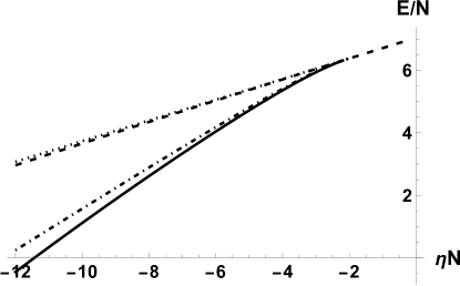
Figure 6: Variational results for asymmetric states with attractive interactions And $\gamma=$10: (Dashed line) The exact energy per particle as a function of interaction $\eta N$ for the symmetric state, and (solid line) the exact asymmetric state. (Dotted line–barely above the exact dashed line) the variational symmetric state; and (dash-dotted line) that for the asymmetric state. The variational bifurcation occurs at $\eta N=-2.3$ compared to the exact result at$-2.07.$

For very large interaction $\eta N$, where the kinetic energy and the external potential become numerically unimportant, the parameter $u$ of Eq. (52) approaches a constant–the wave function no longer changes! Ref. [17] has defined an asymmetry function defined by

$$\Theta=\frac{N_{+}-N_{-}}{N_{+}+N_{-}}$$ (59)

where

$$N_{+} = \int_{-1}^{0}dx\left|\psi(x)\right|^{2}$$ (60)

$$N_{-} = \int_{0}^{1}dx\left|\psi(x)\right|^{2}.$$ (61)

We show $\Theta$ for the exact asymmetric states in Fig. 7. While the large $\eta N$ limit is the same for attractive and repulsive interactions in the variational calculation, there is apparently a difference in that limit for the exact case.

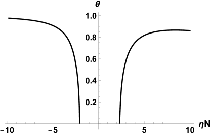
Figure 7: The asymmetry function $\Theta$, Eq. (59) [17] for the exact asymmetric solutions of the GPE as a function of $\eta N$.

IV.4 Approximate numerical method

Numerical solutions of the GPE are, of course, also possible. Such an approach was described for the box-delta external potential in Ref. [17]. We have used the so-called multi-configurational time-dependent Hartree method (MCTDHX) for bosons [27]. This method solves the many-body time-dependent Schr$\mathrm{\ddot{o}}$dinger equation using variational approaches, and is very accurate. The method also allows multiple states to contain condensates. By setting the number of orbitals equal to one (i.e., only the ground state condensate is allowed) one equivalently solves the GPE. It is possible to obtain static as well as dynamic solutions. We simulate the box-delta potential by a Gaussian, as was done in Ref. [17]:

$$V(x)=\frac{\gamma}{\sqrt{\pi\xi}}e^{-x^{2}/\xi^{2}}$$ (62)

with the infinite box walls simulated by a power-law trap:

$$V_{ex}(x)=\left|\frac{x}{L}\right|^{p}$$ (63)

Here $L$ is a length scale and $p$ is an exponent that generates flatness around $x=0$ for $p\gg 1$, $\xi$ is a measure of the width of the Gaussian, and $\gamma$ is the strength parameter we used for the $\delta$-function barrier. To find bifurcation points we solved the time-dependent equations in imaginary time, which gives the ground state, for a range of parameters $\eta$ and $\gamma$ while keeping the number of particles fixed at $N=10.$ The results are presented in Fig. 8. The critical bifurcation point is determined by the position of the kink in the energy.

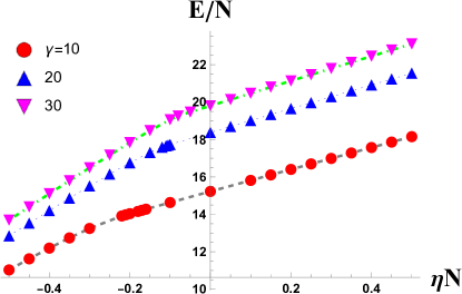
Figure 8: MCTDHX energy per particle E/N versus the interaction parameter $\eta N$ for a number of delta-function strengths $\gamma$. The number of particles is $N=10$. The kink in the graphs gives the bifurcation critical point. The time step taken is usually adjusted by the code itself and is 0.0078125 (unitless) for the present case; the simulation grid has 256 pixels; and the runs are taken over an imaginary time from t=0 to 30 (unitless). The parameters of Eqs. (62) and (63) are $\xi=0.05$, $p=1000$, and $L=0.495$.

IV.5 Bifurcation

In nonlinear equations fixed points often bifurcate; one solution may become unstable while a separate solution becomes stable at that point. Fig. 6 shows the energy per particle for the symmetric and the asymmetric states with the latter separating from the former at $\eta N=-2.07.$ As we step through increasing $\eta N$ values looking for asymmetric parameters, we find that the asymmetric state evolves into the symmetric state in the attractive case precisely at the critical $\eta N$ value. That is, near the critical value the state is almost symmetric, with nearly identical double humps, i.e., $\Theta=0$ there. Note that in the attractive case the energy for the asymmetric state is lower than the corresponding symmetric state, but in the repulsive case it is higher than that of the antisymmetric state. However, that statement does not address the dynamical stability of the states.

We can compare several methods of computing the bifurcations points:

IV.5.1 Variational estimate of bifurcation points

In Sec. IV.3 we showed that the variational method gave the critical $\eta$ value for attractive interactions as

$$\left(\eta N\right)_{c}^{S}=\frac{-\Delta}{3\chi_{22}-\chi_{40}}.$$ (64)

The superscript $S$ notes that the bifurcation is with the symmetric state. For repulsive interactions, we have

$$\left(\eta N\right)_{c}^{AS}=\frac{\Delta}{3\chi_{22}-\chi_{04}}$$ (65)

The bifurcation is with the antisymmetric state. These results are plotted in Fig. 9 as a function of $\gamma$.

IV.5.2 Numerical energy computation

The method described in Sec. IV.4 finds critical bifurcation points in good agreement with the exact values and these are also shown in Fig. 9.

IV.5.3 Estimates of Refs. [17] and [18]

Refs. [17] and [18] consider finding a value of the critical bifurcation interaction parameter for large $\gamma$ by considering approximations for the wave function and for the interaction term. They predict that the the critical interaction parameter will be given by

$$\left(\eta N\right)_{c}^{C}=\frac{8\pi^{2}}{3\gamma}.$$ (66)

This estimate is said be valid for $\gamma\gg 6.$These authors give a treatment valid for small $\gamma$ resulting in the formula

$$\left(\eta N\right)_{c}^{D}=2\ln\left(16/\gamma\right).$$ (67)

Ref. [17] and also gives a numerical treatment with an Gaussian approximation for the barrier and a general variational treatment. In Fig. 9 (Left) we compare our exact values with the MCTDHX numerical results (dots) and the estimates of Eqs. (64) and (66). Fig. 9 (Right) shows exact results compared with Eqs. (64) and (67).

Fig. 10 gives the equivalent results for repulsive interactions where the antisymmetric state bifurcates to an asymmetric wave function.

      

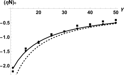
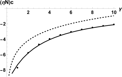
Figure 9: (Left) Values of the critical interaction parameter $\left(\eta N\right)_{c}$ for large $\gamma$ with attractive interactions: (dots) exact computations; (squares) MCTDHX numerical method; (solid line) Eq. (64); (dashed line) Eq. (66). (Right) Values of the critical parameter for small $\gamma$ for attractive interactions: (dots) exact computations; (solid line) Eqs. (64); (dashed line) Eq. (67).

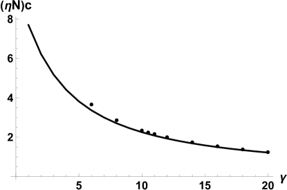
Figure 10: Values of the repulsive critical interaction parameter $\left(\eta N\right)_{c}^{AS}$versus $\gamma$ for the repulsive antisymmetrical state: (dots) exact computations; (solid line) Eq. (65).

V Dynamical Stability

In order to determine the stability of the GPE stationary solutions we carry out a Bogoliubov-type stability analysis as described in Ref. [17]. We consider perturbations of the form

$$\psi(x,t)=\left[\psi_{i}(x)+\delta\psi(x,t)\right]e^{-i\mu t}$$ (68)

where $\delta\psi=u(x)e^{-i\lambda t}+v^{*}(x)e^{i\lambda^{*}t}$; $u$ and $v$ are eigenmodes, and $\lambda$ is the corresponding eigenfrequency. The stability criterion is then $\mathrm{Im}[\lambda]=0$. In Ref. [17] the stability of the symmetric mode was investigated for attractive interactions. Our results for $\gamma=10$ are similar; the symmetric solution becomes unstable beyond the bifurcation point $\eta N\leq-2.07$. Stability analysis of the asymmetric state shows it to be stable, as it should be a standard pitchfork bifurcation. We find no instabilities of the symmetric groundstate with repulsive interactions.

Similarly, we find for $\gamma=10$ the antisymmetric state is unstable for $\eta N$ greater than the bifurcation threshold $+2.338$. For $\gamma=10$ we find no oscillatory instability for attractive interactions. This would seem to differ from Ref. [17], except their reported results were for $\gamma\leq 4$. When we repeat the analysis for $\gamma=1$ we find oscillatory instability at $\eta N<-7.6$ in agreement with their results, and non-oscillatory instability at $\eta N>13.5$. See Figs. 11-13.

There is considerably more that can be said about stability here; indeed we plan a further separate paper on the subject.

Figure 11: Real (solid) and imaginary (dashed) parts of the two lowest eigenfrequencies of Eq. (68) for the symmetric GPE state with $\gamma=10$. The symmetric state is unstable for $\eta N\leq-2.07$. Only the positive parts are shown, the negative parts are identical.

Figure 12: Same as Fig. 11 for the antisymmetric state, also with $\gamma=10$. The antisymmetric state becomes unstable for $\eta N>2.34$.

Figure 13: Eigenfrequencies of the antisymmetric state for $\gamma=1$. At $\eta N=-7.6$ the first and second eigenfrequencies coalesce into complex conjugate pairs, corresponding to oscillatory instability with real frequencies $\pm 10.4$.

VI Discussion

We solved the Gross-Pitaevskii equation for the simple box-$\delta$ external potential analytically for attractive and repulsive interactions in terms of Jacobi elliptic functions. We find symmetric, antisymmetric, and asymmetric functions become the stable states for interaction parameters in appropriate parameter regions. We were able to demonstrate bifurcation from a symmetric state to the asymmetric state below a critical attractive interaction parameter, and from an antisymmetric to an asymmetric state above a critical repulsive interaction. A two-mode variational approximation gives accurate estimates of the critical parameters. An approximate numerical method, the MCTDHX, has also been used to make comparisons between numerical and analytical results and agrees well with the exact results. Comparison demonstrates previous approximate treatments are accurate. A stability analysis shows that the symmetric state becomes unstable below the attractive bifurcation critical point and the antisymmetric state above the repulsive critical point. The antisymmetric state shows an oscillatory instability for attractive interactions within a range of the parameter space. The asymmetric states are stable.

The system can be generalized, for example, to non-symmetrical external potentials for which the bifurcation type may change [11]. There is more to be said concerning stability, which we plan to cover in a future publication. In another subsequent paper we will show the box-$\delta$ potential to be quite convenient for the study of the accuracy of the GPE in comparison with the more general second-quantized Fock Schr$\mathrm{\ddot{o}}$dinger equation.

VII Acknowledgements

We thank Profs. Boris Malomed and Panos Kevrekidis for very useful comments. We also thank Paolo Molignini, Rui Lin, and Axel Lode for use of the MCTDHX code. The MCTDHX calculations were performed at the PARADOX supercomputing facility of the Scientific Computing Laboratory (SCL), Institute of Physics Belgrade, Serbia.

VIII Appendix: Jacobi elliptic functions

We will need the three Jacobi functions $\mathrm{sn}(x|m)$, $\mathrm{cn}(x|m),$ and $\mathrm{dn}(x|m)$ where $y=\mathrm{dn}(x)$ satisfies

$$\frac{d^{2}y}{dx^{2}}+2y^{3}-(2-m)y=0;$$ (69)

$y=\mathrm{sn}(x|m)$ satisfies

$$\frac{d^{2}y}{dx^{2}}-2my^{3}+(1+m)y=0;$$ (70)

and $y=\mathrm{cn}(x|m)$ satisfies

$$\frac{d^{2}y}{dx^{2}}+2my^{3}+(1-2m)y=0.$$ (71)

We also have limits like

$$\mathrm{sn}(x|0)=\sin(x),\mathrm{\qquad sn}(x|1)=\tanh(x),$$ (72)

and the relations

$$\frac{d\mathrm{sn}(x|m)}{dx} = \mathrm{cn}(x|m)\mathrm{dn}(x|m),$$ (73)

$$\frac{d\mathrm{cn}(x|m)}{dx} = -\mathrm{sn}(x|m)\mathrm{dn}(x|m),$$ (74)

$$\frac{d\mathrm{dn}(x|m)}{dx} = -m\mathrm{sn}(x|m)\mathrm{cn}(x|m),$$ (75)

$$\mathrm{sn}(x|m)^{2}+\mathrm{cn}(x|m)^{2} = 1,$$ (76)

$$\mathrm{dn}(x|m)^{2} = 1-m\mathrm{sn}(x|m)^{2}.$$ (77)

Another important quantity is $K(m),$ the complete elliptic integral of the first kind:

$$K(m)=\int_{0}^{\pi/2}\frac{d\phi}{\sqrt{1-m\sin^{2}\phi}},$$ (78)

where $0<m<1$, which determines the period of the Jacobi functions as in

$$\mathrm{sn}(x+2nK(m)|m)=(-1)^{n}\mathrm{sn}(x|m),$$ (79)

where $n$ is an integer. The elliptic integral of the second kind is also used above:

$$E(m)=\int_{0}^{\pi/2}d\phi\sqrt{1-m\sin^{2}\phi}.$$ (80)

The Jacobi epsilon function has the integral representation

$$\mathcal{E}(m)=\int_{0}^{\mathrm{sn}(x|m)}\sqrt{\frac{1-m^{2}t^{2}}{1-t^{2}}}.$$ (81)

References

- [1] G. J. Milburn, J. Corney, E. M. Wright, D. F. Walls, “Quantum dynamics of an atomic Bose-Einstein condensate in a double-well potential,” Phys. Rev. A 55, 4318 (1997).
- [2] R. W. Spekkens and J. E. Sipe, “Spatial fragmentation of a Bose-Einstein condensate in a double-well potential,” Phys. Rev. A 59, 3868 (1999).
- [3] D. J. Masiello, S. B. McKagan, and W. P. Reinhardt, “Multiconfigurational Hartree-Fock theory for identical bosons in a double well potential,” Phys. Rev. A 72, 063624 (2005).
- [4] D. J. Masiello and W. P. Reinhardt, “Symmetry-Broken Many-Body Excited States of the Gaseous Atomic Double-Well Bose-Einstein Condensate,” J. Phys. Chem. A 123, 1962-1967 (2019).
- [5] S. Raghavan, A. Smerzi, S. Fantoni, and S. R. Shenoy, “Coherent oscillations between two weakly coupled Bose-Einstein condensates: Josephson effects, oscillations, and macroscopic self-trapping,” Phys. Rev. A 59, 620 (1999).
- [6] W. J. Mullin, A. R. Sakhel, and R. J. Ragan, “Progressive quantum collapse,” Amer. J. Phys. 90, 200 (2022).
- [7] E. A. Ostrovskaya, Y. S. Kivshar, M. Lisak, B. Hall, F. Cattani, and D. Anderson, “Coupled-mode theory for Bose-Einstein condensates,” Phys. Rev. A 61, 031601(R) (2000).
- [8] P. Coullet and N. Vandenberghe, “Chaotic self-trapping of a weakly irreversible double Bose condensate,” Phys. Rev. E, 64, 025202(R) (2001).
- [9] K. W. Mahmud, J. N. Kutz, and W. P. Reinhardt, “Bose-Einstein condensates in a one-dimensional double square well: Analytical solutions of the nonlinear Schrdinger equation,” Phys. Rev. A 66, 063607 (2002).
- [10] J. Adriazola, R. Goodman, and P. Kevrekidis, “Efficient Manipulation of Bose-Einstein Condensates in a Double-Well Potential,” Comm. in Nonlinear Sci. Numer. Simul. 122, 107219 (2023).
- [11] G. Theocharis, P. G. Kevrekidis, D. J. Frantzeskakis, and P. Schmelcher, “Symmetry breaking is symmetric and asymmetric double-well potentials,” Phys. Rev. E 74, 056608 (2006).
- [12] A. Smerzi, S. Fantoni, S. Giovanazzi, and S.R. Shenoy, “Quantum Coherent Atomic Tunneling between Two Trapped Bose-Einstein Condensates,” Phys. Rev. Lett. 79, 4950 (1997).
- [13] Roberto D’Agosta and Carlo Presilla, “States without a linear counterpart in Bose-Einstein condensates,” Phys. Rev. A 65, 043609 (2002).
- [14] R. K. Jackson and M. I. Weinstein, “Geometric Analysis of Bifurcation and Symmetry Breaking in a Gross-Pitaevskii Equation,” J. Stat. Phys. 116, 881 (2004).
- [15] Thawatchai Mayteevarunyoo, Boris A. Malomed, and Guangjiong Dong, “Spontaneous symmetry breaking in a nonlinear double-well structure,” Phys. Rev. A 78, 053601 (2008).
- [16] B. A. Malomed, ed. “Spontaneous Symmetry Breaking, Self-Trapping, and Josephson Oscillations,” (Springer -Verlag: Berlin and Heidelberg, 2013.
- [17] Elad Shamriz, Nir Dror, and Boris A. Malomed, “Spontaneous symmetry breaking in a split potential box,” Phys. Rev. E 94, 022211 (2016).
- [18] Boris A. Malomed, “Spontaneous Symmetry Breaking in Nonlinear Systems: An Overview and a Simple Model.” In “Nonlinear Dymanics: Materials, Theory, and Experiment,” eds. M. Tlidi and M. Clerk, pp. 97-112 Springer-Heidelberg 2016 and arXiv:1511.08340v1 [nlin.PS]; “Symmetry breaking in laser cavities,” Nature Photonics 9, 287 (2015).
- [19] C. Green, G. B. Mindlin, E. J. D’Angelo, H. G. Solari, and J. R. Tredicce, “Spontaneous Symmetry Breaking in a Laser: The Experimental Side,” Phys. Rev. Lett., 65, 3124 (1990).
- [20] C. Cambournac, T. Sylvestre, H. Maillotte, B. Vanderlinden, P. Kockaert, Ph. Emplit, and M. Haelterman, “Symmetry-Breaking Instability of Multimode Vector Solitons,” Phys. Rev. Lett. 89, 083901 (2002).
- [21] P. G. Kevrekidis, Zhigang Chen, B. A. Malomed, D. J. Frantzeskakis, and M. I. Weinstein, “Spontaneous symmetry breaking in photonic lattices: Theory and Experiment,” Phys. Lett. A 340, 275 (2005).
- [22] Philippe Hamel, Samir Haddadi, Fabrice Raineri, Paul Monnier, Gregoire Beaudoin, Isabelle Sagnes, Ariel Levenson and Alejandro M. Yacomotti, “Spontaneous mirror-symmetry breaking in coupled photonic-crystal nanolasers,” Nature Photonics 9, 311 (2015).
- [23] Tilman Zibold, Eike Nicklas, Christian Gross, and Markus K. Oberthaler, “Classical Bifurcation at the Transition from Rabi to Josephson Dynamics,” Phys. Rev. Lett. 105, 204101 (2010).
- [24] L. D. Carr, Charles W. Clark, and W. P. Reinhardt, “Stationary solutions of the one dimensional nonlinear Schrdinger equation. I. Case of repulsive nonlinearity”, Phys. Rev. A 62, 063610 (2000).
- [25] L. D. Carr, Charles W. Clark, and W. P. Reinhardt, “Stationary solutions of the one-dimensional nonlinear Schrdinger equation. II. Case of attractive nonlinearity,” Phys. Rev. A 62, 063611 (2000).
- [26] A. D. Jackson, G. M. Kavoulakis, and E. Lundh, “Stability of solutions of the Gross-Pitaevskii equation,” Phys. Rev. A 72, 053617 (2005).
- [27] O. E. Alon, A. I. Streltsov, and L. S. Cederbaum, “Multiconfigurational time-dependent Hartree method for bosons: Many-body dynamics of bosonic systems,” Phys. Rev. A 77, 033613 (2008).
- [28] B. A. Malomed, “Variational Treatments in nonlinear fiber optics and related fields,” Progr. Optics 43, 69 (2002).
- [29] Steven Strogatz, “Nonlinear Dynamics and Chaos: With applications to Physics, Biology, Chemistry and Engineering,” Perseus Books, 2000.
- [30] A. R. Sakhel, R. J. Ragan. and W. J. Mullin, “Accuracy of the Gross-Pitaevskii Equation in a Double-Well Potential,” (in preparation).