Exploring Adversarial Threat Models
in Cyber Physical Battery Systems

Abstract

Technological advancements like the Internet of Things (IoT) have facilitated data exchange across various platforms. This data exchange across various platforms has transformed the traditional battery system into a cyber physical system. Such connectivity makes modern cyber physical battery systems vulnerable to cyber threats where a cyber attacker can manipulate sensing and actuation signals to bring the battery system into an unsafe operating condition. Hence, it is essential to build resilience in modern cyber physical battery systems (CPBS) under cyber attacks. The first step of building such resilience is to analyze potential adversarial behavior, that is, how the adversaries can inject attacks into the battery systems. However, it has been found that in this under-explored area of battery cyber physical security, such an adversarial threat model has not been studied in a systematic manner. In this study, we address this gap and explore adversarial attack generation policies based on optimal control framework. The framework is developed by performing theoretical analysis, which is subsequently supported by evaluation with experimental data generated from a commercial battery cell.

I Introduction

I-A Cyber Physical Battery Systems

Technological advancements like IoT, advanced communication systems, and cloud computing protocols have enabled remote control of batteries, transforming traditional batteries into cyber physical systems having various advantages. For example, smart distributed control of power grids’ Battery Energy Storage Systems (BESS), battery energy management in connected autonomous vehicles, etc. Industries like General Motors and Bosch have developed a few cloud-based wireless Battery Management Systems (BMSs) approaches to improve the efficiency of batteries [1][2].

I-B Motivation

Despite numerous benefits, extensive communication networks make BMS vulnerable to cyber attacks. An adversary can have access to multiple attack surfaces and corrupt the transmitted voltage and current data - manipulating the power requirements and current drawn. In [3], a review of cyber security aspects of smart charging management systems of Electric Vehicles (EV) is provided. The work in [4] talks about cyber threats in BESSs. A framework to assess the impacts of cyber attacks in EVs is developed in [5]. The most common results of these cyber attacks are over-charging leading to thermal runaway and battery explosion and over-discharging leading to insufficient power delivery.

Few works proposed solutions to the cyber physical security of BMSs. In [6], cybersecurity of corrupting State-of-Charge (SOC) data of EV battery’s is explored for which the authors trained a Back Propagation Neural Network and tested on experimental dataset to estimate battery SOC under nominal and attacked settings. A Convolutional Neural Network based framework to detect and classify attacked battery sensor data and communication data is proposed in [7]. The work in [8] attempts to address the issue of cybersecurity of plug-in EV using mathematical conditions of stealthy cyber attacks and developing model-based attack detection schemes.

I-C Need for Adversarial Threat Models

However, most of these aforementioned approaches do not focus on understanding the adversarial dynamics. Adversarial dynamics refers to the process followed by the adversary to develop the attacks which can then be injected in the system. In [9], modeling the adversarial dynamics is described in detail. Such modeling efforts are needed to understand the dynamics of the adversarial attacks in the first place which gives us intuition into the decision-making process of the adversaries and then using that information we can develop and deploy technological countermeasures. The modeling process essentially involves designing the attack signals so that the adversarial objectives are satisfied. One of the major objectives of the adversaries is to remain stealthy. Stealthiness means that the attack is not reflected at the user’s end even though the attack may have already been injected by the adversary. Understanding the adversarial dynamics helps us greatly in such scenarios to design resilient control strategies.

Adversarial attack modeling is very similar to modeling a disturbance in any given system. For example, in the estimation method Kalman filtering, the system is assumed to have modeling uncertainties and measurement noise. These noises are modeled by tuning a few parameters of the filter that are associated with the noise. With this knowledge of noise, the Kalman filter gives the most accurate predictions of the system dynamics. Similarly in an adversarial attack scenario, attack inputs from the adversarial are like external noises to the system. Having a model that describes its behavior makes it more like an informed noise as opposed to an arbitrary entity, enabling the next step - accurate estimation of states. The modeling of adversarial attacks can be helpful in gaining information on the attacker’s input behavior beforehand which will help in designing the next step - however, as opposed to estimation in a Kalman filter, the next step in this case would be utilizing the information on adversarial attacks through the developed models to design counterattack measures.

In [8], stealthy attack generation is briefly discussed which captures the relationship between input and output attacks for stealthiness. However, a systematic analysis on the following topics is missing: (i) how such input attack can be formulated based on some high-level adversarial objectives, and (ii) how incorrect model knowledge of adversaries affects this attack formulation process.

In light of the aforementioned research needs and gaps, the main contribution of this work is as follows: This paper explores adversarial threat models in CPBS by analyzing cyber attack generation policies with high-level adversarial objectives and stealthiness features. The approach is formulated based on optimal control principles. Theoretical analysis is used to develop the framework. Subsequently, experimental data generated from a commercial battery cell is used to evaluate the effectiveness under real-world scenarios. We re-iterate the main differences between [8] and this paper: (i) The major focus of [8] is attack detection, whereas that of current work is understanding attack injection mechanisms in detail; (ii) current work utilizes an optimal control approach to generate the current attacks, whereas [8] uses an ad-hoc approach; (iii) current work utilizes a combination of open-loop model and real-time feedback output attack generation, whereas [8] uses only an open-loop model-based approach; and (iv) current work utilizes an experimental data and experimentally identified battery model capturing real-world scenarios, whereas [8] uses simulated battery data. The rest of the paper is organized as follows. In section II, we state the problem of cyber attack in battery systems from the perspective of an adversary. Section III describes the methodology for attack generation policies. Section IV discuss the experimental test results. Finally, Section V concludes the paper.

II Problem Statement: Adversarial attacks in Battery Systems

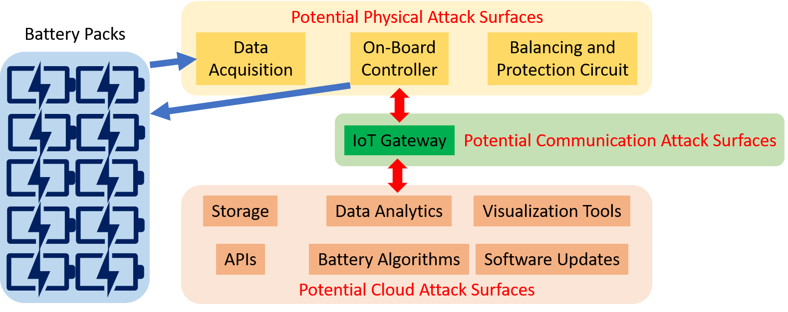
Figure 1: A simplified schematic of cyber physical BESS, adopted and modified from [10].

A simplified architecture of a cyber physical BESS system is shown in Fig. 1. As compared to traditional battery systems which have only one access point, a cyber physical system can be said to have three access points:- (1) Physical access (sensors, onboard controllers, and diagnostic modules, etc.); (2) Communication networks (LTE, 5G, Bluetooth, WiFi, etc and IoT devices); (3) Cloud services (data storage centers, services offered through cloud - like data analytics, visualization tools, firmware updates, etc). All these access points are interconnected as is evident from Fig. 1. Since the attack surface increases due to the interconnections, the CPBS becomes more prone to adversarial attacks.

Due to the presence of WiFi or Bluetooth connectivity, the adversary can eavesdrop into this network from a short distance. The common entry points, devices through which an attacker remotely connect with the system, are service equipment, public-facing infrastructure, vendor cloud service or server, Local Area Network (LAN), WiFi or bluetooth connected devices, meter, software and firmware upgrades, Virtual Private Network (VPN), Virtual Network Computing, etc. [11]. Given the large amounts of security risks faced by CPBS, it is essential to understand the adversarial nature of attackers and hence we focus on the cyber attack perspective. Particularly, we formulate our problem from the point of view of adversaries creating stealthy cyber attacks. This will help us in designing defense strategies against cyber attacks using the knowledge of adversaries obtained by generating stealthy attack policies.

In this work, we analyzed the batteries from a cyber physical realm and generated potential cyber attacks that occur in a CPBS. In general, the only input to a battery system is the input current and the typical measurements from the battery are the voltage measurements and the temperature measurements from a thermocouple. However, in a more simplistic scenario, the only output would be just the voltage measurements. For the current work, the battery system is assumed to be just limited to the current as the only input and voltage measurement as the only output. In such a type of system, the only way for a cyber attacker to attack this CPBS is by introducing attacks in the form of an additional current.

The choice of this additional current injection will cause the system to operate in an undesirable unsafe operating region that can be hazardous. In order to introduce the attack in a stealthy fashion, the obvious effects that will be seen in the output voltage measurements must be mitigated so that the outputs will be as close as to the originally anticipated values. This way, the attack injected will be stealthy and will be undetected. The imperfections in the output measurements will be misunderstood to the measurement noises or any other modeling uncertainties by the user. In short, the main objective of the current work is to propose one of the only few potential ways an attacker can introduce a cyber attack into the CPBS and yet stay stealthy. Leveraging this, one can design potential ways to detect and mitigate such cyber attacks that can be hazardous.

In the current work, we have developed an optimal control strategy to generate adversarial attack policies in the CPBS. Hence it is assumed that the attacker already has the knowledge of the input current profile. The effects of this kind of attack injection that are seen through the output voltage measurement are minimized again by the attacker who will be introducing an attack on the outputs side. A schematic of the potential attack by the cyber attacker in the system of CPBS is illustrated in Fig. 2. It can be seen that the original intended current input to the battery cell is depicted by $I_{nom}$, which however is altered into an actual input $I$ due to the additional attack current $I_{a}$, which is introduced by the cyberattacker. This results in an output voltage of $V$, however again due to the addition of voltage attack $V_{a}$ on the outputs end, the voltage as seen by the battery management systems (BMS) is going to be $V_{mes}$.

Figure 2: Adversarial attack injection into battery systems.

III Adversarial threat model

In this section, we discuss the attack generation mechanisms in detail. First, we describe the battery equivalent circuit model (ECM) which is the basis for model-based attack generation mechanisms. Then, we focus on the optimal control based attack generation.

III-A Description of battery equivalent circuit model (ECM)

A first order ECM [12, 13, 14] is used to model the battery. This includes a set of resistor and capacitor in parallel connected in series with another resistor. This ECM system can be described by a system of equations 2 and 3. First, the ($SoC$) of the battery is modeled by:

$$\dot{SoC}=-\frac{I}{Q}.$$ (1)

Next, the voltage across the capacitor can be written in terms of Kirchoff’s current law as shown in equation 2. Finally, in equation 3 the terminal voltage of the battery is expressed by Kirchoff’s voltage law.

$$\dot{V_{c}}=-\frac{1}{R_{1}C_{1}}V_{c}+\frac{I}{C_{1}}.$$ (2)

$$V_{t}=OCV(SoC)-V_{c}-IR_{0}.$$ (3)

In the equations 2 and 3, $Q$ is the battery capacity in $[A-s]$; $R_{0}$ & $R_{1}$ are the ECM resistances in $[\Omega]$; $C_{1}$ is the ECM capacitance in $[F]$; $V_{c}$, $V_{t}$ & $OCV$ are the voltages in $[V]$, $SoC$ is the battery state of charge.

III-B State-space representation of battery systems

Next, we formulate the ECM equations to a state-space format. The equations (1) and (2) form the state dynamics equation whereas (3) forms the output equation.

$$\dot{X}=AX+BU,$$ (4)

$$Y=g(X,U),$$ (5)

where $X=\begin{bmatrix}SoC&V_{c}\end{bmatrix}^{T}$ is the state vector, $U=I$ is the current input, and $Y=V_{t}$ is the output terminal voltage. The function $g(.)$ is formed by (3) and the $A$ and $B$ matrices are given by:

$$A=\begin{bmatrix}0&0\\ 0&\frac{-1}{R_{1}C_{1}}\end{bmatrix},\ B=\begin{bmatrix}\frac{-1}{Q}\\ \frac{1}{C_{1}}\end{bmatrix}.$$ (6)

In the presence of cyber attacks, we modify (4)-(5) as

$$\dot{X}=AX+B(U_{nom}+U_{a}),$$ (7)

$$Y=g(X,U_{nom}+U_{a})+Y_{a},$$ (8)

where the input $U$ applied to the battery system has two components: $U_{nom}$ is the nominal input applied by the user and $U_{a}$ is the additional input current injected by the attacker. Furthermore, $Y_{a}$ is the output attack injected by the attacker to corrupt the measured voltage $Y$. Next, we discuss potential ways to design the attack signals $U_{a}$ and $Y_{a}$. Specifically, the design of $U_{a}$ will be based on the objective of causing adversarial disturbances. We will consider two cases of adversarial disturbances: (i) overcharging: Here, the adversary will aim to overcharge the battery system with a higher charge value compared to the user’s desirable charge reference. (ii) over-discharging: Here, the adversary will aim to over-discharge the battery system with a lower discharge value compared to the user’s desirable discharge reference. Subsequent to the design of $U_{a}$, the design of $Y_{a}$ will be based on the objective of adversarial stealthiness. In the next two subsections, we will discuss the designs of $U_{a}$ and $Y_{a}$.

III-C Optimal control-based input attack generation

In this subsection, we will discuss the potential design of input attack signals, denoted by $U_{a}$ in (7)-(8). The $U_{a}$ is essentially an additive current signal that is superimposed with user’s intended current signal $U_{nom}$. To this end, the adversary’s objective is to cause either overcharging or over-discharging. Both of these objectives can be formulated as following a reference state trajectory desired by the adversary. This reference trajectory will enable the adversarial requirements of overcharging and over-discharging. Under this scenario, a potential adversarial objective function will be as follows:

$$\min_{U_{a}}J =\frac{1}{2}[X(t_{f})-X_{ref}(t_{f})]^{T}Q_{1}[X(T)-X_{ref}(T)]$$

$$+\frac{1}{2}\int_{t_{0}}^{t_{f}}[X(t)-X_{ref}(t)]^{T}Q_{2}[X(t)-X_{ref}(t)]dt$$

$$+\frac{1}{2}\int_{t_{0}}^{t_{f}}RU_{a}^{2}(t)dt,$$ (9)

where the time window of attack is $t\in[t_{0},t_{f}]$, $X_{ref}$ is a (potentially) time-varying state reference trajectory aiming to either overcharge or over-discharge the battery. The first and second terms on the right hand side of (9) ensure that the actual state $X$ follow the reference $X_{ref}$ as closely as possible during the time period and in the final time $t_{f}$; and the matrices $Q_{1}$ and $Q_{2}$ are adversary-defined weighting matrices. The third term on the right hand side of (9) limits the magnitude of current attack signal $U_{a}$ with a weighting factor $R$. To this end, the goal of the adversary is to minimize the objective function (9) with respect to the dynamic constraints given as system model (7)-(8).

In order to solve the aforementioned optimal control problem, we resort to the the Lagrange multiplier and sweep method discussed in [15, 16]. First, considering the objective function (9) and the state dynamics constraint (7), we construct the Hamiltonian as follows [15, 16]:

$$H(t) =\frac{1}{2}[X(t)-X_{ref}(t)]^{T}Q_{2}[X(t)-X_{ref}(t)]$$

$$+\frac{1}{2}\lambda^{T}[AX(t)+BU_{a}(t)+BU_{nom}(t)],$$ (10)

where $\lambda$ is the Lagrange multiplier. Subsequently, the co-state equations are given by:

$$\frac{\partial H}{\partial U_{a}}=0\implies RU_{a}+B^{T}\lambda=0\implies U_{a}=-R^{-1}B^{T}\lambda,$$ (11)

$$\frac{\partial H}{\partial X}=-\dot{\lambda}\implies Q_{2}[X-X_{ref}]+A^{T}\lambda=-\dot{\lambda},$$ (12)

To solve these two co-state equations (11) and (12), $\lambda$ is chosen of the form $\lambda=SX-V$, where $S$ and $V$ are variables to be determined [15, 16]. Upon taking the derivative of this equation with respect to time, we get the following form:

$$\dot{\lambda}=\dot{S}X+S\dot{X}-\dot{V}$$

$$\implies \dot{\lambda}=\dot{S}X+S[AX+BU_{a}+BU_{nom}]-\dot{V}$$ (13)

Upon substituting the expression of $\dot{\lambda}$ and ${\lambda}$ into (12), we get

$$Q_{2}[X-X_{ref}]+A^{T}[SX-V]$$

$$=-\dot{S}X-S[AX-BR^{-1}B^{T}(SX-V)+BU_{nom}]+\dot{V}.$$ (14)

The equation (14) can be decoupled as two Riccati equations:

$$\dot{V}+A^{T}V-SBR^{-1}B^{T}V-SBU_{nom}+QX_{ref} =0,$$ (15)

$$\dot{S}+SA-SBR^{-1}B^{T}S+A^{T}S+Q =0$$ (16)

The boundary conditions are computed to be:

$$S(T)=Q_{1},$$ (17)

$$V(T)=Q_{1}X_{ref}(T)$$ (18)

Solving (15)-(16) will give us $S$ and $V$, and subsequently, we can compute $U_{a}$ as

$$U_{a}=-R^{-1}B^{T}[SX-V].$$ (19)

III-D Open-loop model and real-time feedback-based output attack generation

Once the input current attack is generated, the next focus is on achieving stealthiness. That is, the adversary’s goal is not to trigger any alarm when the input attack is injected. To achieve such stealthiness, the adversary designs an output attack signal $Y_{a}$ which corrupts the measured terminal voltage, as shown in (8). This attack signal $Y_{a}$ is generated in a way such that the effect of $U_{a}$ is cancelled by $Y_{a}$ at the terminal voltage output.

For this output attack generation, the adversary utilizes the knowledge of system model (7)-(8). To this end, $Y_{a}$ is generated such that the following condition is satisfied:

$$Y=Y_{nom},$$

$$\implies g(X,U_{nom}+U_{a})+Y_{a}=g(X_{nom},U_{nom}),$$

$$\implies Y_{a}=g(X_{nom},U_{nom})-g(X,U_{nom}+U_{a}),$$ (20)

where $X$ is generated by solving $\dot{X}=AX+B(U_{nom}+U_{a})$, $X_{nom}$ is generated by solving $\dot{X}_{nom}=AX_{nom}+BU_{nom}$, and $Y_{nom}=g(X_{nom},U_{nom})$ is the output under no attack condition. The condition (20) ensures that the measured output $Y$ under the attack should resemble to the output $Y_{nom}$ under user-applied nominal input $U_{nom}$.

However, finding the output attack $Y_{a}$ using only the open-loop model (7)-(8) has a limitation. That is, if the model knowledge is inaccurate (as dictated by the ECM model parameters), the output attack will not be able to cancel the effect of input attack. To remedy such limitation, the adversary can potentially use the real-time feedback of $Y$ to correct the inaccuracies of open-loop model generated output attack. Accordingly, the output attack generation will be modified as:

$$Y_{a}=g(X_{nom},U_{nom}) -g(X,U_{nom}+U_{a})$$

$$+K_{a}(Y-g(X_{nom},U_{nom})),$$ (21)

where $Y$ is the measured real-time terminal voltage, and the added second term on the right hand side is the feedback term that corrects the inaccuracies in the open-loop model generated attack signal. The parameter $K_{a}$ is a feedback gain determined to achieve acceptable amount of correction.

IV Results and Discussion

In this section, we evaluate the proposed threat model using experimental data. First, we discuss the identification of the battery model given in Section III.A from the experimental data. Subsequently, we generate the attack signals and evaluate their efficacy. All the experimental data was generated at 25 ${}^{o}C$ temperature in a controlled manner in ESPEC thermal chamber. The input current profile and the output voltage are given and measured by the ARBIN Battery Testing equipment. MITS Pro is the software that has been used to generate schedules for the experiments. An illustration of the experimental setup is depicted in Fig. 3.

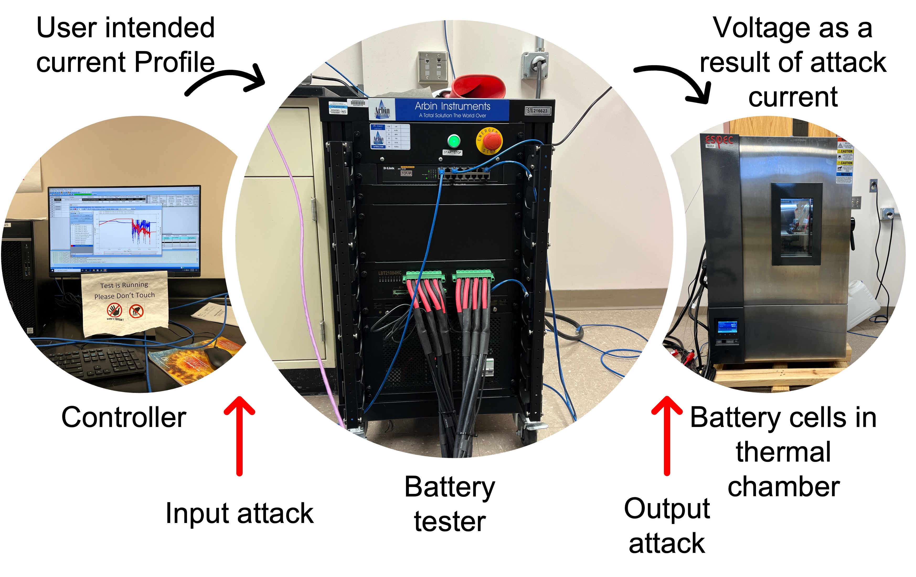
Figure 3: Experimental setup.

For this study, we considered a battery cell with 4.2V to 2.5V operating voltages and rated capacity of 4000 mAh. To identify the battery model parameters, first the open circuit voltage ($OCV$) of the battery has been experimentally investigated by charging and discharging the battery cell with very low current. Subsequently, the equivalent circuit parameters $Q$, $R_{0}$, $R_{1}$ and $C_{1}$ are calculated using the Reference Performance Test (RPT) and the identified parameter values are as follows: (1) $Q=1.4322\times 10^{4}[A-s]$; (2) $R_{0}=1.3513\times 10^{-2}[\Omega]$; (3) $R_{1}=1.028\times 10^{-2}[\Omega]$; (4) $C_{1}=5.2584\times 10^{3}[F]$.

After which these parameters are tuned further using a dynamic current profile, generated from the Urban Dynamometer Driving Schedule (UDDS) velocity profile, as shown in Fig. 4 (top part). A comparison of the experimental voltage and model-generated voltage is shown in Fig. 4 (bottom part).

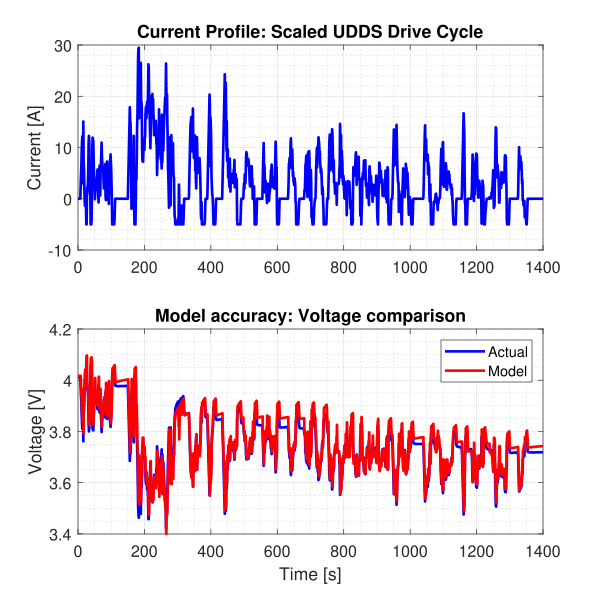
Figure 4: Dynamic current profile and comparison of experimental and model output voltages (RMSE- 0.0483 V).

To illustrate the effectiveness of the proposed threat model or attack generation approach, we will use the following test cases where the current profiles are derived from UDDS and US06 velocity profiles:

• Test Case 1: Modified UDDS-based profile where user-intended discharging is 80% to 50% $SoC$. The adversary’s intent is to over-discharge to 20% $SoC$.

• Test Case 2: Modified US06-based profile where user-intended charging is 20% to 50% $SoC$. The adversary’s intent is to overcharge to 80% $SoC$.

In these aforementioned test cases, the input current attacks are generated using the optimal-control strategy described in Section III-C. Subsequently, the output voltage attacks are generated as discussed in Section III-D, using the combination of the open-loop model and real-time voltage feedback. Next, we illustrate the results for these test cases.

In Fig. 5, the results for Test Case 1 are shown. In Fig. 5(b), the “User-intended current” profile is shown. The generated input “Current attack” is shown in Fig. 5(a), which serves the purpose of over-discharging the battery to 20% $SoC$, ultimately leading to the applied “Current under adversarial input attack” shown in Fig. 5(b). As a result, the battery is being over-discharged, as shown by the “voltage under only input attack” plot in Fig. 5(c) and “SoC under adversarial attack” in Fig. 5(d). Both of these plots indicate that the battery is being over-discharged. Next, to realize stealthiness, output “Voltage attack” is generated, as shown in Fig. 5(a). This output voltage attack is added to the “voltage under only input attack” to generate “voltage under both input and output attack”. As can be seen from Fig. 5(c), the “voltage under both input and output attack” and “Nominal voltage under no attack” are very close to each other, thereby making the attack scenario almost indistinguishable from the no attack scenario.

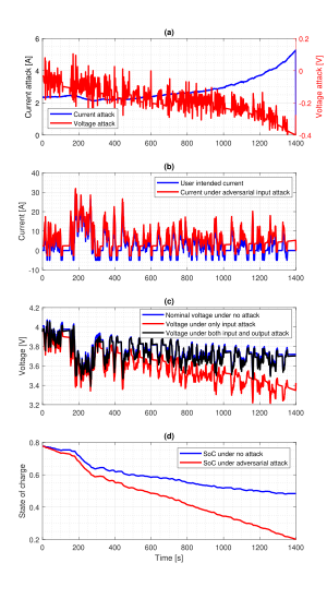
Figure 5: Attack signals and resulting voltage, current, and State-of-Charge for Test Case 1. (a) Current and voltage attack signals; (b) user-intended current and adversarial current; (c) voltages under nominal scenario and various attacks; (d) State-of-Charge under attack and nominal conditions.

Similarly, the results for Test Cases 2 are shown in Fig. 6. Fig. 6 (a) is the illustration of the input as well as output attack components for a charging profile derived from the US06 velocity profile. Fig. 6 (b) is the illustration that depicts the original user-intended current profile as well as the modified current profile under the adversarial input attacks.

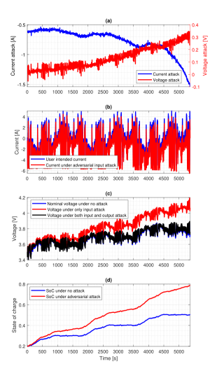
Figure 6: Attack signals and resulting voltage, current, and State-of-Charge for Test Case 2. (a) Current and voltage attack signals; (b) user-intended current and adversarial current; (c) voltages under nominal scenario and various attacks; (d) State-of-Charge under attack and nominal conditions.

V Conclusion

This preliminary study explores the adversarial threat models for CPBS. Within this CPBS setup, potential adversaries can manipulate battery current and terminal voltage to inject harmful which are at the same time stealthy cyber attacks. The goal of this work is to create a form of threat model that can be used to design attack detection and mitigation strategies in battery systems. Here, optimal control principle is used to generate different input attack currents to overcharge or over-discharge the battery. After that, a combination of an open-loop model and real-time feedback is used to generate the output voltage attacks to potentially mask the effect of the input attack. These profiles are then tested on a commercial battery to evaluate their effectiveness.

References

- [1] “General motors’ future electric vehicles to debut industry’s first wireless battery management system.” [Online]. Available: https://news.gm.com/newsroom.detail.html/Pages/news/us/en/2020/sep/ 0909-wbms.html
- [2] “Battery in the cloud.” [Online]. Available: https://www.bosch-mobility-solutions.com/en/solutions/software-and-services/battery-in-the-cloud/battery-in-the-cloud/
- [3] N. Bhusal, M. Gautam, and M. Benidris, “Cybersecurity of electric vehicle smart charging management systems,” in 2020 52nd North American Power Symposium (NAPS). IEEE, 2021, pp. 1–6.
- [4] N. Kharlamova, S. Hashemi, and C. Træholt, “The cyber security of battery energy storage systems and adoption of data-driven methods,” in 2020 IEEE Third International Conference on Artificial Intelligence and Knowledge Engineering (AIKE). IEEE, 2020, pp. 188–192.
- [5] S. Sripad, S. Kulandaivel, V. Pande, V. Sekar, and V. Viswanathan, “Vulnerabilities of electric vehicle battery packs to cyberattacks,” arXiv preprint arXiv:1711.04822, 2017.
- [6] S. Rahman, H. Aburub, Y. Mekonnen, and A. I. Sarwat, “A study of ev bms cyber security based on neural network soc prediction,” in 2018 IEEE/PES Transmission and Distribution Conference and Exposition (T&D). IEEE, 2018, pp. 1–5.
- [7] H.-J. Lee, K.-T. Kim, J.-H. Park, G. Bere, J. J. Ochoa, and T. Kim, “Convolutional neural network-based false battery data detection and classification for battery energy storage systems,” IEEE Transactions on Energy Conversion, vol. 36, no. 4, pp. 3108–3117, 2021.
- [8] S. Dey and M. Khanra, “Cybersecurity of plug-in electric vehicles: Cyberattack detection during charging,” IEEE Transactions on Industrial Electronics, vol. 68, no. 1, pp. 478–487, 2020.
- [9] I. J. Martinez-Moyano, R. Oliva, D. Morrison, and D. Sallach, “Modeling adversarial dynamics,” in 2015 Winter Simulation Conference (WSC), 2015, pp. 2412–2423.
- [10] T. Kim, D. Makwana, A. Adhikaree, J. S. Vagdoda, and Y. Lee, “Cloud-based battery condition monitoring and fault diagnosis platform for large-scale lithium-ion battery energy storage systems,” Energies, vol. 11, no. 1, p. 125, 2018.
- [11] R. D. Trevizan, J. Obert, V. De Angelis, T. A. Nguyen, V. S. Rao, and B. R. Chalamala, “Cyberphysical security of grid battery energy storage systems,” IEEE Access, vol. 10, pp. 59 675–59 722, 2022.
- [12] E. Barsoukov, J. H. Kim, C. O. Yoon, and H. Lee, “Universal battery parameterization to yield a non-linear equivalent circuit valid for battery simulation at arbitrary load,” Journal of power sources, vol. 83, no. 1-2, pp. 61–70, 1999.
- [13] B. Y. Liaw, G. Nagasubramanian, R. G. Jungst, and D. H. Doughty, “Modeling of lithium ion cells—a simple equivalent-circuit model approach,” Solid state ionics, vol. 175, no. 1-4, pp. 835–839, 2004.
- [14] X. Hu, S. Li, and H. Peng, “A comparative study of equivalent circuit models for li-ion batteries,” Journal of Power Sources, vol. 198, pp. 359–367, 2012.
- [15] F. L. Lewis, D. Vrabie, and V. L. Syrmos, Optimal control. John Wiley & Sons, 2012.
- [16] A. Bryson and Y.-C. Ho, “Applied optimal control, hemisphere,” New York, 1975.