Orthogonal Time-Frequency-Space (OTFS) and Related Signaling

Abstract

The principle of orthogonal time-frequency-space (OTFS) signaling is firstly analyzed, followed by explaining that OTFS embeds another signaling scheme referred to as orthogonal short-time Fourier (OSTF). Then, the relationship among OTFS, OSTF, orthogonal frequency-division multiplexing (OFDM) and single-carrier frequency-division multiple-access (SC-FDMA) is explored, demonstrating that OSTF/OTFS are fundamentally the extensions of OFDM/SC-FDMA from one-dimensional (1D) signaling to two-dimensional (2D) signaling. Hence, the characteristics and performance of OSTF/OTFS schemes can be perceived from the well-understood OFDM/SC-FDMA schemes. Accordingly, the advantages and disadvantages of OSTF/OTFS are discussed. Furthermore, from the principles of OFDM/SC-FDMA, the multiuser multiplexing in OSTF/OTFS systems is analyzed with respect to uplink and downlink, respectively. Added on this, a range of generalized multiplexing schemes are presented, whose characteristics are briefly analyzed.

I Introduction

In Chapter 1, the principle of OFDM has been analyzed, showing that OFDM has a range of advantages. With the aid of a suitable cyclic prefix (CP), OFDM is free from inter-symbol interference (ISI), when communicating over frequency-selective fading channels. In OFDM, one-tap frequency (F)-domain equalization is enough to remove the effect of channel fading, making it desirably low-complexity for implementation. In OFDM, the frequency-selective fading channel is converted to a set of flat-fading channels, which may experience correlated or independent fading. Owing to this, if transmitter is designed to employ channel state information (CSI), it can dynamically load different subcarriers with different amount of information according to their channel states, to increase system’s spectral-efficiency. Furthermore, power-allocation can be optimized across subcarriers according to their channel states, so as to meet different design objectives, as shown in Chapter 3. In multiuser OFDM, referred to as orthogonal frequency-division multiple-access (OFDMA), systems, independently faded channels are highly feasible for the implementation of resource-allocation, including both subcarrier- and power-allocation, among users, which enables to achieve significant multiuser diversity gain, as demonstrated in Chapter 4. Owing to the above-mentioned merits, OFDM became the dominate signaling scheme in both 4G and 5G standards.

OFDM also has its disadvantages. As analyzed in Chapter 1, it has the PAPR problem, which imposes extra demand on transceiver design. OFDM signal may experience inter-carrier interference (ICI), if transmitter/receiver’s oscillators are not sufficiently synchronized, or if channel experiences Doppler-spread due to the mobilities of transmitter, receiver or/and communication environments. OFDM needs the help of CP to mitigate ISI, which penalizes system’s spectral-efficiency. When communicating over time-invariant frequency-selective fading channels, it can be shown that ICI is mild and the penalty of adding CP is light. However, wireless channels may be highly time-varying. This is especially the case when considering the future wireless networks, where various high-speed transportation systems, satellite networks, etc., are integrated to support global seamless coverage. Moreover, future wireless systems are expected to be operated over a widely spanning bands, from sub-6G to millimeter wave (mmWave) to Terahertz (THz) bands. Consequently, wireless channels may experience severe Doppler-spread, resulting in the highly time-varying channels, which generate big impacts on the transceiver design and performance of wireless systems.

Specifically, in high Doppler-spread communication environments, the ICI in OFDM systems becomes severe, which demands a high-complexity equalizer to mitigate the resulted effect. While this is a problem, an even worse one may be from the required CP. In OFDM transmission, at least each OFDM symbol is required to be time-invariant, i.e., each OFDM symbol’s duration should be less than channel’s coherence time, which is the reciprocal of two timing the maximum Doppler-spread. Hence, when a channel becomes more time-variant, its coherence time becomes shorter, which in turn requires to shorten the duration of OFDM symbols. Consequently, given that channel’s maximum delay-spread is fixed and hence the CP length is fixed, the duration for information transmission within one OFDM symbol period then has to be shortened. Explicitly, this increases the overhead for CP and hence reduces system’s spectral-efficiency, which can be significant in fast time-varying environments. Moreover, it also has the following consequences. To reduce the duration of information transmission, if system bandwidth keeps fixed, the number of subcarriers has to be reduced to protect their orthogonality. Consequently, individual subband’s bandwidth needs to be increased, which is vulnerable to frequency-selective fading. Alternatively, if the number of subcarriers is fixed, individual subband’s bandwidth has to be increased, and also system’s bandwidth. In this case, the orthogonality of subcarriers cannot be guaranteed, resulting in the increased ICI, especially, when there is also big Doppler-spread.

It can be understood that OFDM is an one-dimensional (1D) signaling scheme, using mainly signal processing in F-domain to conquer the frequency-selective fading resulted from channel’s delay-spread. When wireless channel conflicts simultaneously both frequency-selective fading and time-selective fading (resulted from Doppler-spread), the 1D signaling schemes operated in either the conventional time (T)-domain or F-domain (like OFDM) present deficiencies. Instead, two-dimensional (2D) signaling schemes are desirable to simultaneously deal with the effects generated by channel’s delay- and Doppler-spread. With this motivation, this section considers the 2D signaling schemes, including the orthogonal short-time Fourier (OSTF) [1, 2] and orthogonal time-frequency-space (OTFS) [3, 4] schemes. We will show that OSTF represents the extension of OFDM, while OTFS is the extension of the OFDM’s companion scheme, namely single-carrier frequency-division multiple-access (SC-FDMA). Hence, from OFDM and SC-FDMA and their relationship, we can gain knowledge about the characteristics and performance of OSTF and OTFS. Furthermore, we can be inferred the feasibility of OSTF and OTFS for the implementation of resource-allocation, and which resource-allocation schemes provided in previous chapters may be extended for application in OSTF and OTFS systems. Additionally, in this section, the generalizations of OSTF and OTFS are considered and a range of related schemes for uplink/downlink multiuser scenarios are presented and briefly analyzed.

II Principles of Orthogonal Time-Frequency-Space (OTFS)

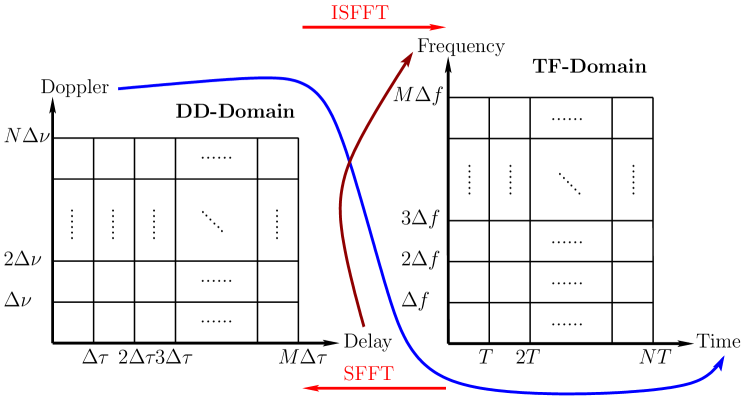
Figure 1: OTFS signaling relationship between DD-domain and TF-domain.

Assume a signal-antenna transmitter sending information to a single-antenna receiver for simplicity to focus on the principles of OTFS. Assume that information symbols are sent in blocks of each block consisting of $MN$ symbols over a channel having the total bandwidth $B$. The block-duration is expressed as $T_{B}$. To facilitate OTFS signaling, the bandwidth $B$ is divided into $M$ subbands of each having a bandwidth $\Delta f=B/M$; the block-duration $T_{B}$ is divided into $N$ time-slots of each with a duration of $T=T_{B}/N$, forming the time-frequency (TF)-grid as shown at the right-side of Fig. 1. It is assumed that $T\Delta f=1$ to protect the orthogonality [3, 5]. With these settings, it is known that the delay resolution and Doppler resolution of the OTFS signals are $\Delta\tau=1/B=1/M\Delta f$ and $\Delta\nu=1/T_{B}=1/NT$, respectively [6].

Assume that the channel’s maximum delay-spread satisfies $\tau_{\max}\leq T$ and the channel’s maximum Doppler-spread is limited to $|\nu_{\max}|\leq\Delta f/2$. Corresponding to the TF-grid, using the delay and Doppler resolutions, the delay-Doppler (DD)-plan in the region of $\left(\tau\in[0,T]\times\nu\in[-\Delta f/2,\Delta f/2]\right)$ is divided into the grid as shown at the left-side of Fig. 1, where on the delay-axis, each division accounts for a delay-spread difference of $\Delta\tau$ and on the Doppler-axis, each division represents a Doppler-spread difference of $\Delta\nu$. In Fig. 1, the relationships between the delay-spread/Doppler-spread in delay-Doppler (DD)-domain and the subbands/time-slots in time-frequency (TF)-domain are explicitly illustrated. For clarity, in the analysis below, the $m$-related indices, i.e., $\tilde{m}$ and $m$, are used for delay-spread and subbands, while the $n$-related indices, i.e., $\tilde{n}$ and $n$, are used for Doppler-spread and time-slots. $\tilde{x}[~{}~{}]$ and $\tilde{y}[~{}~{}]$ are in DD-domain, and $X[~{}~{}]$ and $Y[~{}~{}]$ are in TF-domain.

Figure 2: Modulation and demodulation signaling in OTFS principles.

Following [3, 4, 5, 7], the principles of OTFS can be summarized as follows. Assume that a block of $MN$ data symbols, such as QAM/PSK symbols, are to be transmitted. These symbols are mapped to a $(N\times M)$ grid, as shown by the left-side one in Fig. 1, corresponding to a $(N\times M)$-dimensional matrix $\tilde{\boldsymbol{X}}$, with the element on row $\tilde{n}$ and column $\tilde{m}$ expressed as $\tilde{x}[\tilde{n},\tilde{m}]$. As shown in Fig. 2, $\tilde{\boldsymbol{X}}$ is mapped to a $(M\times N)$-dimensional matrix $\boldsymbol{X}$ in TF-domain via the inverse symplectic finite Fourier transform (ISFFT) [3, 4], with the $(m,n)$-th element expressed as

$$X[m,n]= \frac{1}{\sqrt{MN}}\sum_{\tilde{m}=0}^{M-1}\sum_{\tilde{n}=0}^{N-1}\tilde{x}[\tilde{n},\tilde{m}]\exp\left(j2\pi\left[\frac{n\tilde{n}}{N}-\frac{m\tilde{m}}{M}\right]\right)$$

$$~{}~{}m=0,1,\ldots,M-1;~{}~{}n=0,1,\ldots,N-1$$ (1)

It can be shown that in matrix form, we have

$$\boldsymbol{X}=\boldsymbol{\mathcal{F}}_{M}\tilde{\boldsymbol{X}}^{T}\boldsymbol{\mathcal{F}}^{H}_{N}$$ (2)

where $\boldsymbol{\mathcal{F}}$ are the normalized FFT matrix defined in (1.15) in Chapter 1.

As shown in Fig. 2, then, the Heisenberg transform, also referred to as orthogonal short-time Fourier (OSTF) transform [8, 1, 2, 9], is executed to transform the signals from TF-domain to T-domain for transmission, which generates the T-domain transmit signal as

$$s(t)=\sum_{n=0}^{N-1}\sum_{m=0}^{M-1}X[m,n]g_{tx}(t-nT)\exp\left(j2\pi m\Delta f[t-nT]\right)$$ (3)

In (3), $g_{tx}(t)$ is the pulse-shaping filter of TF modulation, which is defined in $(0,T]$ and normalized to have unit power, i.e., $T^{-1}\int_{0}^{T}|g(t)|^{2}dt=1$. Furthermore, the transmit pulse $g_{tx}(t)$ and its corresponding receive pulse $g_{rx}(t)$ satisfy the bi-orthogonality expressed as [3, 4]

$$\int_{nT}^{(n+1)T} g^{*}_{rx}(t-n^{\prime}T)\exp\left(-j2\pi m^{\prime}\Delta f[t-n^{\prime}T]\right)g_{tx}(t-nT)$$

$$\times\exp\left(j2\pi m\Delta f[t-nT]\right)dt=\delta[n-n^{\prime}]\delta[m-m^{\prime}]$$ (4)

where $\delta[\cdot]$ is the Dirac delta function.

From the TF-grid, we know that the TF resources can provide

$$\frac{T_{B}}{\frac{1}{B}}=\frac{NT}{\frac{1}{M\Delta f}}=MNT\Delta f=MN$$ (5)

degrees of freedom (DoFs). Hence, there are $MN$ independent basis waveforms available. Correspondingly, (3) explains that the $MN$ elements of $\boldsymbol{X}$ are modulated onto the $MN$ OSTF basis waveforms given by [1]

$$\phi_{m,n}(t)= g_{tx}(t-nT)\exp\left(j2\pi m\Delta f[t-nT]\right)$$

$$~{}~{}m=0,1,\ldots,M-1;~{}~{}n=0,1,\ldots,N-1$$ (6)

Assume that a time-varying channel is characterized by the complex baseband impulse response $h(\tau,\nu)$ in the DD-domain. When $s(t)$ of (3) is transmitted over this channel, the received signal is then given by

$$r(t)=\int\int h(\tau,\nu)s(t-\tau)e^{j2\pi\nu(t-\tau)}d\tau d\nu+n(t)$$ (7)

where $n(t)$ is Gaussian noise.

At receiver, as shown in Fig. 2, $r(t)$ is transformed to TF-domain using the Wigner transform, which implements the 2D matched-filtering to compute the ambiguity function as [9]

$$Y[m,n]=\int_{nT}^{(n+1)T}r(t)g_{rx}^{*}(t-nT)\exp\left(-j2\pi m\Delta f[t-nT]\right)dt$$ (8)

It can be shown that $Y[m,n]$ can be expressed as [5]

$$Y[m,n]=\sum_{m^{\prime}=0}^{M-1}\sum_{n^{\prime}=0}^{N-1}H_{m,n}[m^{\prime},n^{\prime}]X[m^{\prime},n^{\prime}]+N[m,n]$$ (9)

where

$$N[m,n]=\int_{nT}^{(n+1)T}n(t)g_{rx}^{*}(t-nT)\exp\left(-j2\pi m\Delta f[t-nT]\right)dt$$ (10)

and

$$H_{m,n} [m^{\prime},n^{\prime}]=\int\int h(\tau,\nu)A_{g_{rx},g_{tx}}[(n-n^{\prime})T-\tau),(m-m^{\prime})\Delta f-\nu]$$

$$\times\exp\left(j2\pi[v+m^{\prime}\Delta f][(n-n^{\prime})T-\tau]\right)\exp\left(j2\pi\nu n^{\prime}T\right)d\tau d\nu$$ (11)

Note that, $H_{m,n}[m^{\prime},n^{\prime}]$ is in fact the coupling generated by the channel between the transmit basis function $\phi_{m^{\prime},n^{\prime}}(t)$ and the receive basis function $\phi_{m,n}(t)$, represented as [2]

$$H_{m,n} [m^{\prime},n^{\prime}]=\int H(\phi_{m^{\prime},n^{\prime}}(t))\phi_{m,n}^{*}(t)dt$$ (12)

with

$$H(\phi_{m^{\prime},n^{\prime}}(t))=\int\int h(\tau,\nu)\phi_{m^{\prime},n^{\prime}}(t-\tau)e^{j2\pi\nu(t-n^{\prime}T-\tau)}d\tau d\nu$$ (13)

For simplicity, assume that the ambiguity function seen in (II) satisfies

$$A_{g_{rx},g_{tx}}[(n-n^{\prime})T-\tau_{\max}),(m-m^{\prime})\Delta f-\nu_{\max}]\approx\delta[n-n^{\prime}]\delta[m-m^{\prime}]$$ (14)

where $\tau_{\max}$ and $\nu_{\max}$ denote the expected maximum delay-spread and Doppler-spread, respectively. Then, the TF-domain channel $H[m,n]$ in (II) can be expressed as

$$H[m,n]= H_{m,n}[m,n]$$

$$= \int\int\exp\left(-j2\pi v\tau\right)h(\tau,\nu)\exp\left(-j2\pi[m\Delta f\tau-n\nu T]\right)d\tau d\nu$$ (15)

When sampling it in DD-domain using $\Delta\tau=1/(M\Delta f)$ and $\Delta\nu=1/(NT)$, we obtain

$$H[m,n]= \sum_{m^{\prime}=0}^{M-1}\sum_{n^{\prime}=0}^{N-1}h\left(m^{\prime},n^{\prime}\right)\exp\left(-j2\pi\left[\frac{mm^{\prime}}{M}-\frac{nn^{\prime}}{N}\right]\right)$$

$$\times\exp\left(-j2\pi\frac{m^{\prime}n^{\prime}}{MN}\right)$$ (16)

where $h(m^{\prime},n^{\prime})=h\left(\frac{m^{\prime}}{M\Delta f},\frac{n^{\prime}}{NT}\right)$. Assume that $h(m^{\prime},n^{\prime})\neq 0$ only when $m^{\prime}\leq L_{\max}$ and $n^{\prime}\leq V_{\max}$, where $L_{\max}$ represents the maximum number of resolvable paths in delay (D)-domain, while $V_{\max}$ represents the maximum number of resolvable paths in Doppler-domain. Then, $h(m^{\prime},n^{\prime})$ with $m^{\prime}=0,1,\ldots,L_{\max}-1$ and $n^{\prime}=0,1,\ldots,V_{\max}-1$ gives the channel’s impulse respond in DD-domain. Correspondingly, (II) is

$$H[m,n]= \sum_{m^{\prime}=0}^{L_{\max}-1}\sum_{n^{\prime}=0}^{V_{\max}-1}h\left(m^{\prime},n^{\prime}\right)\exp\left(-j2\pi\left[\frac{mm^{\prime}}{M}-\frac{nn^{\prime}}{N}\right]\right)$$

$$\times\exp\left(-j2\pi\frac{m^{\prime}n^{\prime}}{MN}\right)$$ (17)

$$= \sum_{m^{\prime}=0}^{L_{\max}-1}\sum_{n^{\prime}=0}^{V_{\max}-1}\tilde{h}\left(m^{\prime},n^{\prime}\right)\exp\left(-j2\pi\left[\frac{mm^{\prime}}{M}-\frac{nn^{\prime}}{N}\right]\right)$$ (18)

where $\tilde{h}\left(m^{\prime},n^{\prime}\right)=h\left(m^{\prime},n^{\prime}\right)\exp\left(-j2\pi\frac{m^{\prime}n^{\prime}}{MN}\right)$. Let $\boldsymbol{H}_{TF}=\{H[m,n]\}$, $\boldsymbol{H}_{DD}=\{h[m,n]\}$ and its modified version $\tilde{\boldsymbol{H}}_{DD}=\{\tilde{h}[m,n]\}$. Explicitly, $\tilde{\boldsymbol{H}}_{DD}$ is known once $\boldsymbol{H}_{DD}$ is known, or vice versa. When $\tilde{\boldsymbol{H}}_{DD}$ is a $(L_{\max}\times V_{\max})$ matrix containing only the elements indexed by $m^{\prime}$ and $n^{\prime}$ in (18), we have

$$\boldsymbol{H}_{TF}= \sqrt{MN}\boldsymbol{\mathcal{F}}_{M}\boldsymbol{\Psi}_{M\times L_{\max}}\tilde{\boldsymbol{H}}_{DD}\boldsymbol{\Psi}^{T}_{N\times V_{\max}}\boldsymbol{\mathcal{F}}_{N}^{H}$$

$$= \sqrt{MN}\boldsymbol{\mathcal{F}}_{M}\tilde{\boldsymbol{H}}_{DD}^{(s)}\boldsymbol{\mathcal{F}}_{N}^{H}$$ (19)

where $\boldsymbol{\Psi}_{M\times L_{\max}}$ is a mapping matrix, constituting the $L_{\max}$ columns of $\boldsymbol{I}_{M}$ corresponding to $m^{\prime}$ seen in (18), and similarly, $\boldsymbol{\Psi}_{N\times V_{\max}}$ is constructed. In (II), $\tilde{\boldsymbol{H}}_{DD}^{(s)}=\boldsymbol{\Psi}_{M\times L_{\max}}\tilde{\boldsymbol{H}}_{DD}\boldsymbol{\Psi}^{T}_{N\times V_{\max}}$ is a $(M\times N)$ sparse matrix, if there are only a small number of paths in DD domain, when compared with $MN$. In this case, it benefits the estimation of TF-selective fading channels in DD-domain with the aid of compressed sensing algorithms [10].

The above analysis and (II) explain that $\boldsymbol{H}_{TF}$, $\boldsymbol{H}_{DD}$ and $\tilde{\boldsymbol{H}}_{DD}$ are equivalent, provided that the ranks of the matrices on the left and right sides of (II) can satisfy the requirements of $M\geq L_{\max}$ and $N\geq V_{\max}$. When one of them is known, the other two can be mathematically derived. Below are two special forms.

First, when channel only experiences delay-spread resulted frequency-selective fading but no Doppler-spread resulted time-selective fading, we have $N=1$ and $n^{\prime}=0$. In this case, (II) is reduced to

$$H[m]= \sum_{m^{\prime}=0}^{L_{\max}-1}h\left(m^{\prime}\right)\exp\left(-j2\pi\left[\frac{mm^{\prime}}{M}\right]\right),~{}m=0,1,\ldots,M-1$$ (20)

Accordingly, $H[m]$ is the fading gain of the $m$th subcarrier of an OFDM system with $M$ subcarriers, as seen in Section 1.5 of Chapter 1. When $L_{\max}\leq M/2$, the $M$ subcarrier channels exist correlation, as analyzed in Section 1.5. Corresponding to (II), $\boldsymbol{h}_{F}=\sqrt{M}\boldsymbol{\mathcal{F}}_{M}\boldsymbol{\Psi}_{M\times L_{\max}}{\boldsymbol{h}}_{D}$ builds the fading relationship between D-domain and F-domain, where $\boldsymbol{h}_{F}$ and ${\boldsymbol{h}}_{D}$ are column vectors, and ${\boldsymbol{h}}_{D}$ is the channel impulse response (CIR) in D-domain.

Second, when channel only experiences the Doppler-spread resulted time-selective fading, but no delay-spread resulted frequency-selective fading, we have $M=1$ and $m^{\prime}=0$. In this case, (II) is simplified to

$$H[n]= \sum_{n^{\prime}=0}^{V_{\max}-1}h\left(n^{\prime}\right)\exp\left(j2\pi\left[\frac{nn^{\prime}}{N}\right]\right),~{}n=0,1,\ldots,N-1$$ (21)

Correspondingly, $H[n]$ is the fading gain experienced by the $n$th time-slot. Similarly, it can be shown that, when $V_{\max}\leq N/2$, the $N$ time-slots experience correlated fading. Corresponding to (II), $\boldsymbol{h}_{T}=\boldsymbol{\mathcal{F}}_{N}^{H}\boldsymbol{\Psi}_{N\times V_{\max}}\boldsymbol{h}_{D}$ gives the fading relationship between Doppler-domain and T-domain, where $\boldsymbol{h}_{T}$ and ${\boldsymbol{h}}_{D}$ are column vectors, while ${\boldsymbol{h}}_{D}$ is the CIR in Doppler-domain.

Let us now return to (9). When the ambiguity function satisfies the condition of (14), $H_{m,n}[m^{\prime},n^{\prime}]$ in (II) is non-zero only when $m^{\prime}=m$ and $n^{\prime}=n$. Hence, (9) is simplified to

$$Y[m,n]=H[m,n]X[m,n]+N[m,n],~{} m=0,1,\ldots,M-1;$$

$$n=0,1,\ldots,N-1$$ (22)

showing that there is no interference between the TF-domain symbols sent in TF-domain, revealing the characteristics of OFDM experiencing only frequency-selective fading. However, we should be aware of that this is achieved, only when the condition of (14) is guaranteed. If this is not the case due to the strong selectivity in TF-domain or/and the non-ideal $g_{rx}(t)$ and $g_{tx}(t)$, the detection of TF-domain symbols $X[m,n]$ would experience inter-symbol interference (ISI).

Since at transmitter, data symbols are mapped to the DD-domain grid, as shown in Fig. 1, at receiver, as shown in Fig. 2, the TF-domain signals are converted to the DD-domain using the symplectic finite Fourier transform (SFFT) as

$$\tilde{y}[\tilde{n},\tilde{m}]= \frac{1}{\sqrt{MN}}\sum_{m=0}^{M-1}\sum_{n=0}^{N-1}Y[m,n]\exp\left(-j2\pi\left[\frac{\tilde{n}n}{N}-\frac{\tilde{m}m}{M}\right]\right),$$

$$~{}~{}\tilde{n}=0,1,\ldots,N-1;~{}~{}\tilde{m}=0,1,\ldots,M-1$$ (23)

Upon substituting (II) associated with (II) and (II) into (II), it can be shown that the input-output relationship in DD-domain can be represented as [5, 3, 4]

$$\tilde{y}[\tilde{n},\tilde{m}]= \frac{1}{MN}\sum_{\tilde{m}^{\prime}=0}^{M-1}\sum_{\tilde{n}^{\prime}=0}^{N-1}\tilde{x}[\tilde{n},\tilde{m}]h_{w}[\tilde{m}-\tilde{m}^{\prime},\tilde{n}-\tilde{n}^{\prime}]+\tilde{n}[\tilde{n},\tilde{m}]$$ (24)

where

$$\tilde{n}[\tilde{n},\tilde{m}]= \frac{1}{\sqrt{MN}}\sum_{m=0}^{M-1}\sum_{n=0}^{N-1}N[m,n]\exp\left(-j2\pi\left[\frac{\tilde{n}n}{N}-\frac{\tilde{m}m}{M}\right]\right)$$ (25)

is the Gaussian noise, $h_{w}[l,k]$ is the discrete representation of the DD-domain channel impulse response $h_{w}(\tau,\nu)$ upon considering the effect from the rectangular windowing functions applied at both transmitter and receiver, which can be expressed as

$$h_{w}(\tau,\nu)=\int\int h(\tau^{\prime},\nu^{\prime})w(\tau-\tau^{\prime},\nu-\nu^{\prime})\exp(-j2\pi\nu\tau)d\tau^{\prime}d\nu^{\prime}$$ (26)

with

$$w(\tau,\nu)=\sum_{m=0}^{M-1}\sum_{n=0}^{N-1}\exp\left(-j2\pi[\nu nT-\tau m\Delta f]\right)$$ (27)

Hence,

$$h_{w}[l,k]=h_{w}\left(\frac{l}{M\Delta f},\frac{k}{NT}\right)$$ (28)

Note that, upon discretizing the variables in (26), we have an expression

$$h_{w}(l,k)=\sum_{l^{\prime}=0}^{M-1}\sum_{k^{\prime}=0}^{N-1}h(l^{\prime},k^{\prime})w(l-l^{\prime},k-k^{\prime})\exp\left(-j\frac{2\pi lk}{MN}\right)$$ (29)

The input-output relationship in (24) explains that the observation $\tilde{y}[\tilde{n},\tilde{m}]$ corresponding to $\tilde{x}[\tilde{n},\tilde{m}]$ consists of a linear combination of possibly all the transmitted symbols $\tilde{x}[\tilde{n}^{\prime},\tilde{m}^{\prime}]$. Hence, there is in general ISI, which needs to be mitigated in detection by a suitable equalizer, such as, that is implemented in the principle of minimum mean-square error (MMSE) [1].

III Relationship of OTFS with OSTF, OFDM and SC-FDMA

Now we analyze the relationship of OTFS with some other multicarrier signaling schemes, including the orthogonal short-time Fourier (OSTF) [1, 2], OFDM and single-carrier frequency-division multiple-access (SC-FDMA) [11] schemes. From their relationship, the characteristics of OTFS and OSTF as well as their advantages and disadvantages in applications will become clearer based on our knowledge about SC-FDMA and OFDM. Please refer to [1, 2] for the details of OSTF signaling, the principle of OFDM has been addressed in Chapter 1, while the principle of SC-FDMA can be found in [11], all of which are also inferred in the following texts.

First, according to [1, 2], the OSTF signaling is embedded in the OTFS signaling. It has a system diagram as shown in Fig. 2 after removing the ISFFT at transmitter and SFFT at receiver. Therefore, in OSTF signaling, information symbols are mapped on a $(M\times N)$-grid in TF-domain, and the transmit signal is given by (3), where $X[m,n]$ are data symbols. Alternatively, the OTFS signaling in (3) is reduced to the OSTF signaling, when $\boldsymbol{\mathcal{F}_{M}}$ and $\boldsymbol{\mathcal{F}_{N}}$ are replaced by the identity matrices of corresponding dimensions.

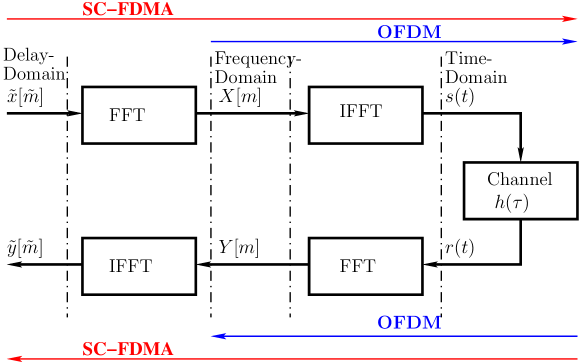
Figure 3: Diagram illustrating the relationship between OFDM and SC-FDMA signaling.

Second, when $N=1$ and assuming that $g_{tx}(t)$ is a rectangular waveform function having unity amplitude, (3) becomes

$$s(t)=\sum_{m=0}^{M-1}X[m]\exp\left(j2\pi m\Delta ft\right)$$ (30)

which is the OFDM signaling. Also, Eq. (20) shows that, when channel has no Doppler-spread, the fading gains of subcarrier channels are given by the FFT on the CIR in D-domain, which agrees with that in OFDM systems, as shown in Section 1.5 of Chapter 1. Hence, OSTF represents the 2D extension of OFDM.

Third, The relationship between OFDM and SC-FDMA is depicted in Fig. 3. Hence, in SC-FDMA systems, $\{X[m]\}$ in (30) are provided by the DFT operating on the data symbols $\{\tilde{x}[\tilde{m}]\}$, i.e., $\boldsymbol{X}=\boldsymbol{\mathcal{F}}\tilde{\boldsymbol{x}}$. Hence, based on the principles of OTFS, we can view that the data symbols in SC-FDMA are mapped to a vector in D-domain.

It is worth noting that, in point-to-pint communications where all resources in TF-domain are assigned to one transmitter, the FFT/IDFT seen in the transmitter of Fig. 3 is meaningless, as $\boldsymbol{\mathcal{F}}\boldsymbol{\mathcal{F}}^{H}=\boldsymbol{I}$. In this case, data symbols $\{\tilde{x}[\tilde{m}]\}$ are directly transmitted in blocks in T-domain, with each block adding a suitable CP to mitigate inter-block interference. In this way, at receiver, after removing the CP and transforming the received signals to F-domain using a FFT, the low-complexity one-tap F-domain equalization can be carried out to mitigate ISI [12, 13], before transforming the signals to D-domain to carry out data detection. In practice, SC-FDMA scheme is typically employed to support the uplink multiuser transmissions [11]. In this regard, each user is assigned a portion of $M_{d}=M/K$ subcarriers, where $K$ denotes the number of users. Correspondingly, at each user’s transmitter, the FFT matrix is $(M_{d}\times M_{d})$ dimensional. After FFT, the $M_{d}$ symbols are mapped to $M_{d}$ out of $M$ subcarriers based on a mapping scheme. Specifically, interleaved mapping, giving the so-called interleaved frequency-division multiple-access (IFDMA), or localized mapping, yielding the localized FDMA (LFDMA), can be implemented. More generally, many other, including random, mapping may also be implemented. The selection between IFDMA and LFDMA is depended on the design objective of attaining frequency diversity gain or benefit from resource-allocation, which will be further discussed later in conjunction with OTFS/OSTF.

Based on the relationship between OFDM and SC-FDMA and that between OFDM and OSTF, it is easy to show that OTFS is reduced to SC-FDMA, when $N=1$ and assuming that $g_{tx}(t)$ is rectangular with unity amplitude. This can be seen from (II) and (2). Specifically, when $N=1$, (2) becomes $\boldsymbol{X}=\boldsymbol{\mathcal{F}}\tilde{\boldsymbol{x}}$, which is the FFT operation implemented in the SC-FDMA transmitter, as shown in Fig. 3. Hence, OTFS represents the 2D extension of SC-FDMA.

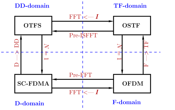
Figure 4: Diagram illustrating the relationship among OTFS, OSTF, OFDM and SC-FDMA.

In summary, the relationship among OTFS, OSTF, OFDM and SC-FDMA can be depicted as Fig. 4, where FFF $\leftarrow\boldsymbol{I}$ means that FFT matrix is replaced by identity matrix, D$\rightarrow$DD and F$\rightarrow$TF denote the generalization from D-domain to DD-domain and from F-domain to TF-domain, respectively, ‘Pre-FFT’ means that the inputs to OFDM are preprocessed by FFT, and ‘Pre-ISFFT’ indicates that the inputs to OSTF are preprocessed using ISFFT.

IV Multiuser Multiplexing and Resource-Allocation in OTFS and OSTF Systems

Having shown the mirror relationship between OTFS/OSTF and SC-FDMA/OFDM in Section III, let us now analyze the multiuser multiplexing and resource-allocation in OTFS and OSTF systems. For convenience of description, assume $M_{d}=M/K_{d}$ and $N_{D}=N/K_{D}$, where $M_{d}$, $N_{D}$, $K_{d}$ and $K_{D}$ are all integers. Then, a block of resources provided by the $(N\times M)$-grid in DD-domain or provided by the $(M\times N)$-grid in TF-domain can be simultaneously allocated to $K_{d}K_{D}$ users. Each user can be assigned $M_{d}N_{D}$ units of resources or DoFs.

For analysis, the CIR in DD-domain is expressed as

$$h(\tau,\nu)=\sum_{l=0}^{\mathcal{L}}h_{l}\delta(\tau-\tau_{l})\delta(\nu-\nu_{l})$$ (31)

where $\mathcal{L}$ denotes the number of physical propagation paths (rays), and $h_{l}$, $\tau_{l}$ and $\nu_{l}$ represent the gain, delay and Doppler-shift of the $l$th path. Often, $l=0$ corresponds to the line-of-sight (LoS) path, while the others are reflected paths.

In a richly scattered dispersive channel operated in relatively low frequency bands, such as sub-6GHz, $\mathcal{L}$ may be a very big number. When $\mathcal{L}>>L_{\max}V_{\max}$, where $L_{\max}$ and $V_{\max}$ are defined in association with (II), the CIR can be expressed as

$$h(\tau,\nu)=\sum_{l=0}^{L_{\max}-1}\sum_{d=0}^{V_{\max}-1}h(l,d)\delta\left(\tau-\frac{l}{M\Delta f}\right)\delta\left(\nu-\frac{d}{NT}\right)$$ (32)

explaining that the channel can be resolved into $L_{\max}V_{\max}$ independent paths. Each resolvable path is a combination of many paths closely related in terms of delay and Doppler-shift. Each path has a fading gain of $h(l,d)$, which statistically obeys, such as, complex Gaussian distribution or other distribution, depended on the communications environments. The total power conveyed to receiver by the resolvable paths is

$$P_{r}=\sum_{l=0}^{L_{\max}-1}\sum_{d=0}^{V_{\max}-1}\|h(l,d)\|^{2}$$ (33)

which can be exploited by receiver when it coherently combines, such as, using maximum ratio combining (MRC)[14], all the resolvable paths in DD-domain. It can be demonstrated that $P_{r}$ converges to a constant, when $L_{\max}V_{\max}$ increases.

Figure 5: Illustration of a time-frequency selective wireless channel.

In a sparsely scattered channel operated in high-frequency, such as mmWave, bands, the number of physical paths from transmitter to receiver may be very small. For this kind of channels, the CIR can be expressed by (31), where $h_{l}$ is a complex number. The total power conveyed to receiver is

$$P_{r}=\sum_{l=0}^{\mathcal{L}}\|h_{l}\|^{2}$$ (34)

which can be exploited by receiver when it is capable of distinguishing the individual paths and coherently combines them in DD-domain. $P_{r}$ is a constant and invariant unless transmitter, receiver or/and environment change.

In the TF-domain, as seen in (II) and (II), the channel $H[m,n]$ of each TF-element is a linear combination of the physical propagation paths with different delays and Doppler-shifts. Hence, $H[m,n]$ is a random process whose varying rate is dependent on both delays and Doppler-shifts. Typically, it has the characteristics as shown in Fig. 5. The TF-elements close to each other experience correlated fading, but those separated in TF-domain at least by $1/M\Delta f$ or/and $1/NT$ experience independent fading.

Below the multiuser multiplexing is discussed in the preference of uplink and downlink, respectively, although a scheme may often be similarly implemented for both uplink and downlink. It is generally assumed that the transmissions to/from different users are synchronous. To support the analysis, the DD-domain grid and TF-domain grid with $16\times 8$ resource units as shown in Fig. 6 will be referred to. In this example, we set $M_{d}=4$ and $N_{D}=2$, meaning that each user is assigned $4\times 2$ units of resources in either DD-domain or TF-domain. When the corresponding SC-FDMA and OFDM are considered, the first row in DD-domain grid and the first column in TF-domain grid are referred to, and each user is assigned $M_{d}=4$ resource units.

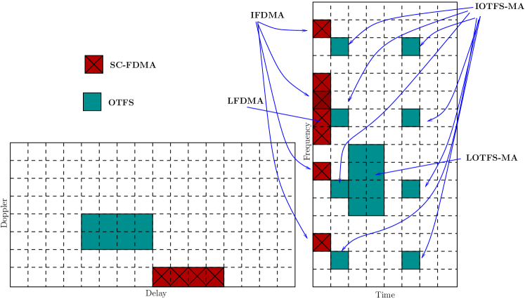
Figure 6: Resource-distribution in OTFS and SC-FDMA multiuser systems.

IV-A Uplink

SC-FDMA was proposed mainly for supporting the uplink transmission in 4G LTE/LTE-A systems. Hence, let us start with the existing multiplexing (multiple-access) schemes used in SC-FDMA systems [11]. As previously mentioned, SC-FDMA has two types of mapping protocols from D-domain to F-domain, yileding IFDMA and LFDMA. Assume that $\tilde{\boldsymbol{x}}_{k}$ is a $M_{d}$-length data symbol vector. For both IFDMA and LFDMA, the signals mapped to the $M$ subbands (subcarriers) can be written as

$$\boldsymbol{x}_{k}=\boldsymbol{P}^{(k)}_{M\times M_{d}}\boldsymbol{\mathcal{F}}_{M_{d}}\tilde{\boldsymbol{x}}_{k}$$ (35)

where $\boldsymbol{\mathcal{F}}_{M_{d}}$ is the $(M_{d}\times M_{d})$ FFT matrix, $\boldsymbol{P}^{(k)}_{M\times M_{d}}$ is a $(M\times M_{d})$ mapping matrix, which constitutes $M_{d}$ columns chosen from $\boldsymbol{I}_{M}$ according to the subbands assigned to a user. Specifically for user $k=2$ shown in the figure, the mapping matrix for LFDMA is

$$\boldsymbol{P}^{T}_{16\times 4}=\setcounter{MaxMatrixCols}{16}\begin{bmatrix}0&0&0&0&0&0&0&0&1&0&0&0&0&0&0&0\\ 0&0&0&0&0&0&0&0&0&1&0&0&0&0&0&0\\ 0&0&0&0&0&0&0&0&0&0&1&0&0&0&0&0\\ 0&0&0&0&0&0&0&0&0&0&0&1&0&0&0&0\end{bmatrix}$$ (36)

and for IFDMA is

$$\boldsymbol{P}^{T}_{16\times 4}=\setcounter{MaxMatrixCols}{16}\begin{bmatrix}0&0&1&0&0&0&0&0&0&0&0&0&0&0&0&0\\ 0&0&0&0&0&0&1&0&0&0&0&0&0&0&0&0\\ 0&0&0&0&0&0&0&0&0&0&1&0&0&0&0&0\\ 0&0&0&0&0&0&0&0&0&0&0&0&0&0&1&0\end{bmatrix}$$ (37)

The mapping matrix has the property $\left(\boldsymbol{P}^{(k)}_{M\times M_{d}}\right)^{T}\boldsymbol{P}^{(k)}_{M\times M_{d}}=\boldsymbol{I}_{M_{d}}$.

Generalizing to OTFS, let $\tilde{\boldsymbol{X}}_{k}$ be the $(N_{D}\times M_{d})$ data symbol block in DD-domain to be transmitted by user $k$. Then, the signals mapped to TF-domain grid can be expressed as

$$\boldsymbol{X}_{k}=\boldsymbol{P}^{(k)}_{M\times M_{d}}\boldsymbol{\mathcal{F}}_{M_{d}}\tilde{\boldsymbol{X}}_{k}^{T}\boldsymbol{\mathcal{F}}_{N_{D}}^{H}\boldsymbol{P}^{(k)}_{N_{D}\times N}$$ (38)

where $\boldsymbol{P}^{(k)}_{N_{D}\times N}$ is a mapping matrix with its $N_{D}$ rows chosen from $\boldsymbol{I}_{N}$ according to the time-slots assigned to user $k$, which is similar as (36) or (37), and has the property of $\boldsymbol{P}^{(k)}_{N_{D}\times M}\left(\boldsymbol{P}^{(k)}_{N_{D}\times M}\right)^{T}=\boldsymbol{I}_{N_{D}}$. Similar to LFDMA, when the mapping matrices $\boldsymbol{P}^{(k)}_{M\times M_{d}}$ and $\boldsymbol{P}^{(k)}_{N_{D}\times M}$ have the structure of (36), the OTFS can be termed as LOTFS-MA. Similar to IFDMA, when the mapping matrices $\boldsymbol{P}^{(k)}_{M\times M_{d}}$ and $\boldsymbol{P}^{(k)}_{N_{D}\times M}$ have the structure of (37), the OTFS can be termed as IOTFS-MA. In Fig. 6, the examples of mappings in LOTFS-MA and IOTFS-MA are illustrated.

Following IFDMA and LFDMA, it is expected that LOTFS- and IOTFS-MA have the following properties:

• As there is a FFT from D-domain to F-domain and an IFFT from F-domain to T-domain, as IFDMA/LFDMA, each user’s transmit power is focused on one frequency, resulting in single-carrier transmission. Hence, it contributes to PAPR reduction. By contrast, there is only an IFFT of $\boldsymbol{\mathcal{F}}_{N_{D}}^{H}$ from Doppler-domain to T-domain, which generates PAPR dynamics. Hence, it can be expected that the transmit signals of a user fluctuates in T-domain with respect to time-slots. Due to this $N_{D}$-point IFFT, the PAPR of user’s transmit signals is $N_{D}$.

• IOTFS-MA implements fixed TF-domain resource-allocation, while in LOTFS-MA systems, blocks of TF-domain resources may be assigned to different users dynamically.

• Hence, from Fig. 5 we can be inferred that IOTFS-MA systems may attain TF-diversity gain but no multiuser diversity gain. By contrast, LOTFS-MA systems may not gain benefit from channel’s TF-selectivity but can enjoy multiuser diversity via TF-domain resource-allocation.

• The maximum diversity order achievable by IOTFS-MA systems is limited by $M_{d}N_{D}$, and $L_{\max}V_{\max}$ in richly scattered channels or $\mathcal{L}$ in sparsely scattered channels. In LOTFS-MA systems, the diversity gain is mainly relied on the number of users.

• In IOTFS-MA, when transmitter has channel knowledge, the mapping matrices can be replaced by the one obtained from the dynamic TF-domain resource-allocation among $K_{d}K_{D}$ uplink users. In this case, IOTFS-MA is enabled to achieve both TF-diversity and multiuser diversity. The cost for this is the possibly increased PAPR.

In terms of performance, we should expect the following observations, when assuming that the ambiguity function satisfies the condition of (14).

• Since there is no interference in TF-domain, as seen in (II), simple one-tap equalization can be implemented in TF-domain, and yield no multiuser interference (MUI). However, the symbols of one user interfere with each other in DD-domain, generating the intra-user interference (IUI).

• Alternatively, equalization can also be implemented in DD-domain by first mapping $Y[m,n]$ in (II) without TF-domain processing to DD-domain. However, the complexity is higher than that operated in TF-domain, as the equalizer is now $M\times N$ dimensions.

• While IOTFS-MA enables TF-diversity gain and LOTFS-MA also has the potential to provide certain TF-diversity gain, the TF-diversity gain may not be obtained, unless IUI is sufficiently suppressed with the aid of an advanced equalizer/detector, such as, in the principles of MMSE or maximum likelihood.

Instead of the mapping implemented in TF-domain, as shown in (38), the mapping can also be carried out in DD-domain. Correspondingly, we have

$$\boldsymbol{X}_{k}=\boldsymbol{\mathcal{F}}_{M}\boldsymbol{P}^{(k)}_{M\times M_{d}}\tilde{\boldsymbol{X}}_{k}^{T}\boldsymbol{P}^{(k)}_{N_{D}\times N}\boldsymbol{\mathcal{F}}_{N}^{H}$$ (39)

In this way, each user’s data symbols are firstly mapped to $M_{d}N_{D}$ elements of the $(N\times M)$ DD-grid and then a $(M\times N)$-dimensional ISFFT is executed to transform signals from DD-domain to TF-domain. Comparing (39) with (38), which carries out $(M_{d}\times N_{D})$-dimensional ISFFT, we can be implied that the transmitter implementation with the scheme of (38) is less demanding.

Define $\boldsymbol{\mathcal{F}}^{(k)}_{M\times M_{d}}=\boldsymbol{\mathcal{F}}_{M}\boldsymbol{P}^{(k)}_{M\times M_{d}}$, which in fact is a $(M\times M_{d})$ matrix containing the columns of $\boldsymbol{\mathcal{F}}_{M}$ selected by $\boldsymbol{P}^{(k)}_{M\times M_{d}}$. Similarly, defined $\left(\boldsymbol{\mathcal{F}}^{(k)}_{N\times N_{D}}\right)^{H}=\boldsymbol{P}^{(k)}_{N_{D}\times N}\boldsymbol{\mathcal{F}}_{N}^{H}$, which is a $(N_{D}\times N)$ matrix containing the rows of $\boldsymbol{\mathcal{F}}_{N}^{H}$ chosen by $\boldsymbol{P}^{(k)}_{N_{D}\times N}$. Then, (39) is reduced to

$$\boldsymbol{X}_{k}=\boldsymbol{\mathcal{F}}^{(k)}_{M\times M_{d}}\tilde{\boldsymbol{X}}_{k}^{T}\left(\boldsymbol{\mathcal{F}}^{(k)}_{N\times N_{D}}\right)^{H}$$ (40)

Explicitly, the operations can be explained as the 2-D spreading of $\tilde{\boldsymbol{X}}_{k}^{T}$ using the DFT sequences from $\boldsymbol{\mathcal{F}}_{M}$ and $\boldsymbol{\mathcal{F}}_{N}$. Hence, the scheme can be referred to as the ISFFT-spread OSTF, corresponding to the DFT-spread OFDM. To generalize the ISFFT-spread OSTF, (40) can be written as

$$\boldsymbol{X}_{k}=\boldsymbol{\mathcal{S}}^{(k)}_{A}\tilde{\boldsymbol{X}}_{k}^{T}\left(\boldsymbol{\mathcal{S}}^{(k)}_{B}\right)^{T}$$ (41)

where $\boldsymbol{\mathcal{S}}^{(k)}_{A}$ and $\boldsymbol{\mathcal{S}}^{(k)}_{B}$ are general spreading matrices satisfying the requirements for dimensions. This scheme is referred to as TF-spread OSTF, just like F-spread CDMA [11].

The characteristics and performance of ISFFT-spread OSTF and TF-spread OSTF can be summarized as follows.

• While in ISFFT-spread OSTF, data symbols can be viewed to be modulated in DD-domain, in TF-spread OSTF, data symbols are modulated and spread in TF-domain. Hence, TF-spread OSTF belongs to a TF-domain signaling scheme, with ISFFT-spread OSTF being one of its special cases.

• As each symbol is spread to all the elements of TF-grid, full TF-diversity is achievable, when advanced multiuser detectors are employed.

• Fixed resource-allocation (or so-said no resource-allocation) in TF-domain and also in power (P)-domain, except the possible power-control for dealing with the near-far problem.

• Detectors/equalizers need to consider $(M\times N)$ dimensions and hence, it may be high-complexity, especially, when advanced multiuser detection is implemented.

• While ISFFT-spread OSTF signals can be expected to have low PAPR, TF-spread OSTF signals may experience the PAPR problem depending on the spreading sequences employed.

Finally, with the aid of the formula of $\textrm{vec}(\boldsymbol{ABC})=(\boldsymbol{C}^{T}\otimes\boldsymbol{A})\textrm{vec}(\boldsymbol{B})$, where $\otimes$ denotes the Kronecker product, $\textrm{vec}(\cdot)$ represents the vectoring operation, (41) can be written as

$$\textrm{vec}(\boldsymbol{X}_{k})= (\boldsymbol{\mathcal{S}}^{(k)}_{B}\otimes\boldsymbol{\mathcal{S}}^{(k)}_{A})\textrm{vec}(\tilde{\boldsymbol{X}}_{k}^{T})$$ (42)

$$= \boldsymbol{\mathcal{S}}^{(k)}\times\textrm{vec}(\tilde{\boldsymbol{X}}_{k}^{T})$$ (43)

where $\boldsymbol{\mathcal{S}}^{(k)}=(\boldsymbol{\mathcal{S}}^{(k)}_{B}\otimes\boldsymbol{\mathcal{S}}^{(k)}_{A})$. (42) and (43) explain that the transmitter first spreads a $M_{d}N_{D}$-length data vector $\textrm{vec}(\tilde{\boldsymbol{X}}_{k}^{T})$ to obtained a $MN$-length one $\textrm{vec}(\boldsymbol{X}_{k})$, the elements of which are then mapped to the $(M\times N)$-grid in TF-domain.

The difference between (43) and (42)/(41) is that in (42)/(41), the spreading sequences are obtained by concatenating two sets of sequences of length-$M$ and length-$N$, respectively, while in (43), the spreading sequences are from one generalized set of length-$MN$, which includes that in (42)/(41) as a subset. Hence, based on (43), there are more sequences to choose for $\boldsymbol{\mathcal{S}}^{(k)}$ and, consequently, yielding better performance. For example, when binary spreading sequences are considered, the total number of sequences following (42)/(41) is $2^{M+N}$, while that following (43) is $2^{MN}$. Again, we should realized that in the general cases, the detection complexity may be extreme, when $MN$ is a big value.

IV-B Downlink

Downlink transmission is in the fashion of broadcast, i.e., BS sends information simultaneously to all downlink users. Hence, BS carries out all transmit processing and the transmissions to different users are synchronous. Below are some possible downlink signaling and transmission schemes.

Let $\tilde{\boldsymbol{X}}_{k}\in\mathbb{C}^{N_{D}\times M_{d}}$, $k=1,\ldots,K_{d}K_{D}$, be the data symbols to be sent to the downlink users. The first downlink signaling scheme maps these data symbols to the $(N\times M)$ grid in DD-domain. Then, they are ISFFT processed to TF-domain. This can be expressed as

$$\boldsymbol{X}=\boldsymbol{\mathcal{F}}_{M}\left(\sum_{k=1}^{K_{d}K_{D}}\boldsymbol{P}^{(k)}_{M\times M_{d}}\tilde{\boldsymbol{X}}_{k}^{T}\boldsymbol{P}^{(k)}_{N_{D}\times N}\right)\boldsymbol{\mathcal{F}}_{N}^{H}$$ (44)

where $\boldsymbol{P}^{(k)}_{M\times M_{d}}$ and $\boldsymbol{P}^{(k)}_{N_{D}\times N}$ are the mapping matrices assigned to user $k$, which are also used by user $k$ to pick up its detected information from the DD-grid. Equation (44) can be written as

$$\boldsymbol{X}= \sum_{k=1}^{K_{d}K_{D}}\boldsymbol{\mathcal{F}}_{M}\boldsymbol{P}^{(k)}_{M\times M_{d}}\tilde{\boldsymbol{X}}_{k}^{T}\boldsymbol{P}^{(k)}_{N_{D}\times N}\boldsymbol{\mathcal{F}}_{N}^{H}$$

$$= \sum_{k=1}^{K_{d}K_{D}}\boldsymbol{\mathcal{F}}^{(k)}_{M\times M_{d}}\tilde{\boldsymbol{X}}_{k}^{T}\left(\boldsymbol{\mathcal{F}}^{(k)}_{N\times N_{D}}\right)^{H}$$ (45)

where $\boldsymbol{\mathcal{F}}^{(k)}_{M\times M_{d}}$ consists of the $M_{d}$ columns/sequences of $\boldsymbol{\mathcal{F}}_{M}$ while $\boldsymbol{\mathcal{F}}^{(k)}_{N\times N_{D}}$ consists of the $N_{D}$ columns/sequences of $\boldsymbol{\mathcal{F}}_{N}$ assigned to user $k$. Hence, with this downlink signaling scheme, each symbol is spread to all the $MN$ resource units in TF-domain. Therefore, while each user can enjoy the TF-diversity, if it can afford an equalizer of relatively high-complexity, there is no multiuser diversity available from the resource-allocation in TF-domain. Only power-control is needed in response to the transmission distances between users and BS.

Secondly, as (41), the above signaling scheme can be extended to a downlink TF-spread OSTF scheme, which accordingly, has the formula

$$\boldsymbol{X}= \sum_{k=1}^{K_{d}K_{D}}\boldsymbol{\mathcal{S}}^{(k)}_{A}\tilde{\boldsymbol{X}}_{k}^{T}\left(\boldsymbol{\mathcal{S}}^{(k)}_{B}\right)^{T}$$ (46)

Furthermore, following (43), the most general downlink TF-spread scheme generates the TF-domain signals as

$$\textrm{vec}(\boldsymbol{X})= \sum_{k=1}^{K_{d}K_{D}}\boldsymbol{\mathcal{S}}^{(k)}\times\textrm{vec}(\tilde{\boldsymbol{X}}_{k}^{T})$$ (47)

Again, it is worth noting that these spreading schemes cannot gain benefit from the TF-domain resource-allocation to achieve multiuser diversity.

However, it is noteworthy that $\boldsymbol{\mathcal{S}}^{(k)}$ in (47) is very general and can be configured for designing different signaling schemes. For example, $\boldsymbol{\mathcal{S}}^{(k)}$ can be designed to interleave the elements in $\tilde{\boldsymbol{X}}_{k}$ and different users are distinguished by their interleaving matrices. It can be a sparse matrix to implement sparse code-division multiple-access (SCDMA) [15, 16] or sparse-code multiple-access (SCMA) [17, 18]. Or, it is a matrix chosen from a set, which is joined with $\tilde{\boldsymbol{X}}_{k}$ to implement TF-domain index modulation (IM) [19, 20]. It is easy to understand that the indices can be defined on the activities of the elements in $\tilde{\boldsymbol{X}}_{k}$, or the codes in $\boldsymbol{\mathcal{S}}^{(k)}$. Furthermore, a set of matrices of $\{\boldsymbol{\mathcal{S}}^{(k)}\}$ can be designed as modulation indices for each user, and IM is implemented at matrix level. Additionally, when multiple transmit and receive antennas are employed, spatial modulation (SM) [21] based OSTF or preprocessing-SM (PSM) based OSTF [22] can be designed.

The above downlink signaling schemes are designed by assuming that CSI is employed at user receivers, BS only knows the statistical CSI to each of users. When BS also employs the CSI to all users, the spreading in (47) can be replaced by preprocessing as

$$\textrm{vec}(\boldsymbol{X})= \sum_{k=1}^{K_{d}K_{D}}\boldsymbol{\mathcal{P}}^{(k)}\times\textrm{vec}(\tilde{\boldsymbol{X}}_{k}^{T})$$

$$= \boldsymbol{\mathcal{P}}\tilde{\boldsymbol{x}}$$ (48)

where

$$\boldsymbol{\mathcal{P}}= \left[\boldsymbol{\mathcal{P}}^{(1)},\boldsymbol{\mathcal{P}}^{(2)},\ldots,\boldsymbol{\mathcal{P}}^{(K_{d}K_{D})}\right]$$

$$\tilde{\boldsymbol{x}}= \left[\textrm{vec}^{T}(\tilde{\boldsymbol{X}}_{1}^{T}),\textrm{vec}^{T}(\tilde{\boldsymbol{X}}_{2}^{T}),\ldots,\textrm{vec}^{T}(\tilde{\boldsymbol{X}}_{K_{d}K_{D}}^{T})\right]^{T}$$ (49)

with $\textrm{vec}^{T}(\cdot)$ denoting the transpose operation of a vector obtained from vectorization. This gives the third downlink transmission scheme, which carries out transmit preprocessing in TF-domain.

Since in (IV-B), $\boldsymbol{\mathcal{P}}$ is a transmit preprocessing matrix need to be optimized with certain objective under required constraints by exploiting the CSI to different users, the resource-allocation in both TF- and P-domains have to be addressed. For example, BS may first make use the TF-domain DoFs to design a preprocessing matrix $\boldsymbol{\mathcal{P}}^{\prime}$, so that the signals arriving at different users are free of MUI, enabling mobile users to implement low-complexity detection. Then, power is allocated to obtain $\boldsymbol{\mathcal{P}}=\boldsymbol{\mathcal{P}}^{\prime}\boldsymbol{\beta}$, where $\boldsymbol{\beta}$ is a real diagonal matrix for power-allocation to maximize SNR, spectral-efficiency, etc., of the system [11].

Following OFDM, the final downlink transmission scheme considered can be described as

$$\boldsymbol{X}= \sum_{k=1}^{K_{d}K_{D}}\boldsymbol{P}^{(k)}_{M\times M_{d}}\tilde{\boldsymbol{X}}_{k}^{T}\boldsymbol{\beta}_{k}\boldsymbol{P}^{(k)}_{N_{D}\times N}$$ (50)

This is a pure resource-allocation scheme operated in TF-domain, i.e., it is an OSTF scheme. Depended on the expected trade-off between efficiency and complexity, $\boldsymbol{P}^{(k)}_{M\times M_{d}}$, $\boldsymbol{P}^{(k)}_{N_{D}\times N}$ and $\boldsymbol{\beta}_{k}$ may be designed as follows. Firstly, it may do fixed allocation with $\boldsymbol{P}^{(k)}_{M\times M_{d}}$, $\boldsymbol{P}^{(k)}_{N_{D}\times N}$ and $\boldsymbol{\beta}_{k}$ (power-allocation matrix) all fixed for the individual users. Secondly, it may fix the TF-domain resources using fixed $\boldsymbol{P}^{(k)}_{M\times M_{d}}$ and $\boldsymbol{P}^{(k)}_{N_{D}\times N}$ for individual users, but allocate power, i.e., design $\boldsymbol{\beta}_{k}$, to users dynamically. Lastly, it can dynamically allocate both TF-domain resources and power via designing $\boldsymbol{P}^{(k)}_{M\times M_{d}}$, $\boldsymbol{P}^{(k)}_{N_{D}\times N}$ and $\boldsymbol{\beta}_{k}$ according to the CSI to different users, service requirements, and so on. It may implement joint optimization, or carry out TF- and P-domains resource-allocation separately to reduce complexity. For example, BS may first assign each downlink user the TF-domain resources (subbands and time-slots), followed by the power-allocation in the principle of, such as, water-filling. With this regard, the optimization algorithms can be straightforwardly extended from that provided in Chapters 3 and 4.

V Concluding Remarks

The principles of OTFS and its companion OSTF have been analyzed, showing that they represent the 1D-to-2D extensions of SC-FDMA and OFDM, respectively. As SC-FDMA and OFDM, we can be inferred that OTFS and OSTF have their individual advantages and disadvantages that are dependent on application scenarios. Typically, as SC-FDMA able to achieve F-diversity, OTFS is beneficial to obtaining TF-diversity resulted from the delay- and Doppler-spread, leading any DD-domain symbols to attain similar performance. Due to this, OTFS signaling is not feasible for exploiting the DoFs in space (S)-domain, provided by distributed users, to obtain multiuser diversity. By contrast, as OFDM, single TF-domain symbol in OSTF cannot benefit from channel’s frequency- and time-selectivity to get diversity gain. However, the qualities of different TF-domain elements in OSTF can be highly dynamic, which renders resource-allocation to be high-efficiency. OSTF signals in TF-domain are highly time-variant, but have little interference with each other. In contrast, OTFS signals in DD-domain are slowly time-varying signals, but they interfere with each other.

The practical implementations of both OTFS and OSTF face many challenges, but most of them are rooted from channel estimation, i.e., estimating $h(\tau,\nu)$ as accurate as possible and with an overhead as small as possible. Provided that accurate $h(\tau,\nu)$ is available, mapping data in DD-domain or alternatively, in TF-domain is not a critical issue, but mainly dependent on the feasibility of implementation, which is limited by practical communications environments. From the principles of OTFS and OSTF, we can be inferred that for channel estimation, pilot symbols may be arranged in DD-domain [4, 23, 24, 25] or in TF-domain [25], and correspondingly, channels can be estimated in DD-domain or TF-domain. However, it is noteworthy that, regardless of OTFS or OSTF, channels can be estimated either in DD-domain or in TF-domain. This is analogous to SC-FDMA and OFDM, no matter which one it is, the objective of channel estimation is to estimate the CIR in D-domain, which can be implemented either in F-domain or in D-domain. The difference between them is that in D-domain, the estimator aims to recover the accurate $h(\tau)$ by estimating all individual rays. Hence, it is more suitable for estimating the sparse channels having a low number of rays from transmitter to receiver. By contrast, in F-domain, the estimator motivates to find the $h(\tau)$ that can reveal the channel behaviors on different subcarriers, but does not put emphasis on whether the estimated $h(\tau)$ is the true CIR. This is especially suitable for estimating the channels having many multipath components generated by random scatters. Again, which one is more desirable is dependent on the communication environments in practice and other related factors, such as, complexity-efficiency trade-off.

References

- [1] A. M. Sayeed, “How is time frequency space modulation related to short time fourier signaling?” in 2021 IEEE Global Communications Conference (GLOBECOM), 2021, pp. 1–6.
- [2] K. Liu, T. Kadous, and A. Sayeed, “Orthogonal time-frequency signaling over doubly dispersive channels,” IEEE Transactions on Information Theory, vol. 50, no. 11, pp. 2583–2603, 2004.
- [3] R. Hadani, S. Rakib, M. Tsatsanis, A. Monk, A. J. Goldsmith, A. F. Molisch, and R. Calderbank, “Orthogonal time frequency space modulation,” in 2017 IEEE Wireless Communications and Networking Conference (WCNC), 2017, pp. 1–6.
- [4] R. Hadani, S. Rakib, S. Kons, M. Tsatsanis, A. Monk, C. Ibars, J. Delfeld, Y. Hebron, A. J. Goldsmith, A. F. Molisch, and R. Calderbank, “Orthogonal time frequency space modulation,” 2018.
- [5] P. Raviteja, K. T. Phan, Y. Hong, and E. Viterbo, “Interference cancellation and iterative detection for orthogonal time frequency space modulation,” IEEE Transactions on Wireless Communications, vol. 17, no. 10, pp. 6501–6515, 2018.
- [6] P. Bello, “Characterization of randomly time-variant linear channels,” IEEE Transactions on Communications, vol. 11, no. 4, pp. 360 – 393, December 1963.
- [7] Z. Wei, W. Yuan, S. Li, J. Yuan, and D. W. K. Ng, “Transmitter and receiver window designs for orthogonal time-frequency space modulation,” IEEE Transactions on Communications, vol. 69, no. 4, pp. 2207–2223, 2021.
- [8] A. M. Sayeed and B. Aazhang, “Communication over multipath fading channels: A time-frequency perspective,” in Wireless Communication - TDMA versus CDMA, S. G. Glisic and P. L. Leppanen, Eds. Kluwer Academic Publishers, 1997, pp. 73–98.
- [9] L. Cohen, Time-Frequency Analysis. Englewood Cliffs, New Jersey, USA: Prentice Hall PTR, 1995.
- [10] X. Zhang, Matrix Analysis and Applications. Beijing, P.R.China: Tsinghua University Press, 2006.
- [11] L.-L. Yang, Multicarrier Communications. Chichester, United Kingdom: John Wiley, 2009.
- [12] F. Adachi, H. Tomeba, and K. Takeda, “Frequency-domain equalization for broadband single-carrier multiple access,” IEICE Transactions on Communications, vol. E92-B, no. 5, pp. 1441 – 1456, May 2009.
- [13] S. Okuyama, K. Takeda, and F. Adachi, “MMSE frequency-domain equalization using spectrum combining for Nyquist filtered broadband single-carrier transmission,” in 2010 IEEE 71st Vehicular Technology Conference, 2010, pp. 1–5.
- [14] J. G. Proakis, Digital Communications, 5th ed. McGraw Hill, 2007.
- [15] Y. Liu, L.-L. Yang, and L. Hanzo, “Spatial modulation aided sparse code-division multiple access,” IEEE Transactions on Wireless Communications, vol. 17, no. 3, pp. 1474–1487, 2018.
- [16] R. Hoshyar, F. Wathan, and R. Tafazolli, “Novel low-density signature for synchronous CDMA systems over AWGN channel,” IEEE Transactions on Signal Processing, vol. 56, no. 4, pp. 1616–1626, April 2008.
- [17] L. Dai, B. Wang, Y. Yuan, S. Han, I. Chih-lin, and Z. Wang, “Non-orthogonal multiple access for 5G: solutions, challenges, opportunities, and future research trends,” IEEE Communications Magazine, vol. 53, no. 9, pp. 74–81, 2015.
- [18] K. Deka, A. Thomas, and S. Sharma, “OTFS-SCMA: A code-domain NOMA approach for orthogonal time frequency space modulation,” IEEE Transactions on Communications, vol. 69, no. 8, pp. 5043–5058, 2021.
- [19] S. Doğan-Tusha, A. Tusha, S. Althunibat, and K. Qaraqe, “Orthogonal time frequency space multiple access using index modulation,” IEEE Transactions on Vehicular Technology, vol. 72, no. 12, pp. 15 858–15 866, 2023.
- [20] Z. Sui, H. Zhang, Y. Xin, T. Bao, L.-L. Yang, and L. Hanzo, “Low complexity detection of spatial modulation aided OTFS in doubly-selective channels,” IEEE Transactions on Vehicular Technology, vol. 72, no. 10, pp. 13 746–13 751, 2023.
- [21] Y. Yang, Z. Bai, K. Pang, S. Guo, H. Zhang, and K. S. Kwak, “Spatial-index modulation based orthogonal time frequency space system in vehicular networks,” IEEE Transactions on Intelligent Transportation Systems, vol. 24, no. 6, pp. 6165–6177, 2023.
- [22] L.-L. Yang, “Transmitter preprocessing aided spatial modulation for multiple-input multiple-output systems,” in 2011 IEEE 73rd Vehicular Technology Conference (VTC Spring), 2011, pp. 1–5.
- [23] W. Shen, L. Dai, J. An, P. Fan, and R. W. Heath, “Channel estimation for orthogonal time frequency space (OTFS) massive MIMO,” IEEE Transactions on Signal Processing, vol. 67, no. 16, pp. 4204–4217, 2019.
- [24] P. Raviteja, K. T. Phan, and Y. Hong, “Embedded pilot-aided channel estimation for OTFS in delay–doppler channels,” IEEE Transactions on Vehicular Technology, vol. 68, no. 5, pp. 4906–4917, 2019.
- [25] H.-T. Sheng and W.-R. Wu, “Time-frequency domain channel estimation for OTFS systems,” IEEE Transactions on Wireless Communications, pp. 1–1, 2023.