Faster Convergence with Less Communication: Broadcast-Based Subgraph Sampling for Decentralized Learning over Wireless Networks

Abstract

Consensus-based decentralized stochastic gradient descent (D-SGD) is a widely adopted algorithm for decentralized training of machine learning models across networked agents. A crucial part of D-SGD is the consensus-based model averaging, which heavily relies on information exchange and fusion among the nodes. Specifically, for consensus averaging over wireless networks, communication coordination is necessary to determine when and how a node can access the channel and transmit (or receive) information to (or from) its neighbors. In this work, we propose BASS, a broadcast-based subgraph sampling method designed to accelerate the convergence of D-SGD while considering the actual communication cost per iteration. BASS creates a set of mixing matrix candidates that represent sparser subgraphs of the base topology. In each consensus iteration, one mixing matrix is sampled, leading to a specific scheduling decision that activates multiple collision-free subsets of nodes. The sampling occurs in a probabilistic manner, and the elements of the mixing matrices, along with their sampling probabilities, are jointly optimized. Simulation results demonstrate that BASS enables faster convergence with fewer transmission slots compared to existing link-based scheduling methods. In conclusion, the inherent broadcasting nature of wireless channels offers intrinsic advantages in accelerating the convergence of decentralized optimization and learning.

I Introduction

Collaborative machine learning (ML) with decentralized data has gained widespread recognition as a promising solution for preserving data privacy in large-scale ML. In this approach, models are trained directly on individual devices using locally available datasets. Federated learning is a notable example in this category [1]. Traditional studies on federated learning often center around a server-based architecture, wherein locally trained models from distributed agents are periodically aggregated and synchronized at a parameter server. However, this master-worker architecture is susceptible to single node failure and generates high communication load between the server and the agents. An alternative solution to address these challenges is serverless decentralized learning. In this approach, each agent performs local training and communicates with its locally connected neighbor(s) for in-network model fusion. Unlike the server-based architecture, serverless decentralized learning offers advantages such as increased scalability and robustness against single node failures.

Training ML models to perform a certain task is essentially solving an optimization problem. One commonly used first-order optimization algorithm for decentralized learning is the Decentralized Stochastic Gradient Descent (D-SGD) [2, 3]. D-SGD comprises two key components: (1) stochastic gradient descent and (2) consensus-based model averaging. Particularly, the consensus averaging mechanism ensures that the agents can approach a state of agreement on a quantity of interest [4, 5, 6], which is the optimizer of the global objective function.

Convergence analysis of D-SGD has been extensively investigated in the literature [7, 8, 9, 10, 11]. A common understanding is that the communication topology plays a critical role in the convergence performance, which is reflected by the spectral gap of the mixing (or gossip) matrix [12]. Recent studies have examined the impact of topology in the convergence bound and unveiled some counter-intuitive remarks [13, 14]. Focusing on communication aspects, previous works have explored the effects of compression (with quantization or sparsification) [15, 16], link failures [17, 18], communication delays [19], and asynchronous updating [20].

Generally, existing works on communication-efficient D-SGD can be classified into two lines of research. The first line focuses on reducing the amount of information transmitted over the links by compressing the communicated models [15, 21, 22, 23]. The second one focuses on tuning the frequency of communication between nodes, either by link scheduling [24, 25, 26] or with event-triggered communication [27]. These two aspects can also be jointly considered. In this work, we align with the second research line and study the impact of partial communication on the performance of decentralized learning, meaning that not all links need to be used in every iteration. Although this approach may slow down the per-iteration convergence, activating a subset of nodes and links in each iteration can significantly reduce the communication cost or delay. This trade-off has been exploited in the literature and proves advantageous in improving communication efficiency.

I-A Related Works

Most existing works in the literature focus on analyzing and improving the convergence of D-SGD with respect to the number of iterations. When considering the actual communication cost in every iteration, a matching-based link scheduling design named MATCHA has been proposed in [24]. The key idea is to improve the error-versus-wall-clock-time convergence of D-SGD by activating connectivity-critical links more often, given a fixed communication cost (e.g., a specific number of activated links) per iteration. Along this line, a Laplacian matrix sampling approach is presented in [25], where a set of candidate Laplacian matrices are designed and sampled with probabilities subject to a given cost measure. Both works involve optimizing the mixing matrices based on the Laplacian or weighted Laplacian of subgraphs containing the set of scheduled links. However, it is important to note that these approaches primarily focus on link-based scheduling and do not account for the potential impact of broadcast transmission. In wireless networks featuring broadcast transmission, an agent/node can effectively reach all of its neighbors at the cost of one transmission slot, thereby enhancing information dissemination throughout the network. Although distributed optimization with broadcast-based communication has been considered in [28, 29], these works focus on convergence analysis and do not attempt to optimize the communication dynamics.

Our work aims to provide a systematic approach to optimize the communication pattern and mixing matrix weights for D-SGD with broadcast transmission, which has been overlooked in the current literature.

I-B Contributions

The main contributions of the paper are summarized below.

• We propose BASS, a communication-efficient framework for D-SGD with broadcast transmission, using random sampling of sparser subgraphs of the base topology under a given communication cost constraint.

• With our proposed design, we create a set of candidate subgraphs containing multiple collision-free sets and sample one subgraph in each iteration, leading to a specific scheduling decision. We further optimize the mixing matrices of the candidate subgraphs and their sampling probabilities to speed up convergence.

• We present a heuristic approach to reduce the computational complexity, which requires solving only one optimization problem with less communication overhead.

To the best of our knowledge, this is the first work to consider broadcast-based graph sparsification for accelerating convergence of D-SGD measured by objective improvement per transmission slot. Simulation results show that BASS achieves significant performance gain compared to existing link-based scheduling approaches, validating the benefits of exploiting broadcast transmission in the communication design.

II Preliminaries on Decentralized Optimization and Learning

II-A Basic Introduction to Graphs

We consider a network of $N$ nodes, modeled as an undirected and connected graph $\mathcal{G}=(\mathcal{N},\mathcal{E})$, with $\mathcal{N}=\{1,\ldots,N\}$ being the set of nodes/agents, and $\mathcal{E}\subseteq\{(i,j)\in\mathcal{N}\times\mathcal{N}|i\neq j\}$ being the set of links/edges. Each node $i$ can only communicate with its set of neighbors, denoted as $\mathcal{N}_{i}=\{j|(i,j)\in\mathcal{E}\}$. The degree of a node $i$ is $d_{i}=|\mathcal{N}_{i}|$, which represents the number of its neighbors.

The topology of the graph $\mathcal{G}$ can be represented by its adjacency matrix $\mathbf{A}\in\mathbb{R}^{N\times N}$. The elements of $\mathbf{A}$ are $A_{ij}=1$ if $(i,j)\in\mathcal{E}$ and $A_{ij}=0$ otherwise, with $A_{ii}=0,\forall i$. The Laplacian matrix of $\mathcal{G}$ is defined as $\mathbf{L}=\mathbf{D}-\mathbf{A}$, where $\mathbf{D}=\text{diag}(d_{1},...,d_{N})$ is a diagonal matrix whose diagonal elements are the node degrees. We will refer to $\mathbf{D}$ as the degree matrix of the graph $\mathcal{G}$. The Laplacian matrix has the sum of each row/column equal to zero, i.e., $\mathbf{L}\mathbf{u}=\mathbf{0}$, and $\mathbf{u}^{\top}\mathbf{L}=\mathbf{0}$, where $\mathbf{u}$ and $\mathbf{0}$ are column vectors of all-ones and all-zeros, respectively.

II-B Collaborative Machine Learning in Decentralized Setting

Let $\mathbf{x}\in\mathbb{R}^{d}$ represent the learning model. The objective of collaborative training can be written as the following optimization problem

$$\min_{\mathbf{x}\in\mathbb{R}^{d}}\left(F(\mathbf{x}):=\frac{1}{N}\sum_{i=1}^{N}F_{i}(\mathbf{x})\right),$$ (1)

where each $F_{i}:\mathbb{R}^{d}\rightarrow\mathbb{R}$ defines the local objective function of agent $i$. For model training, the local objective $F_{i}$ can be defined as the expected local risk/loss function

$$F_{i}(\mathbf{x}):=\mathbb{E}_{s\sim\mathcal{D}_{i}}f(\mathbf{x};s),$$ (2)

where $\mathcal{D}_{i}$ refers to the local data distribution at agent $i$, and $f(\mathbf{x};s)$ is the loss function of the learning model $\mathbf{x}$ for sample $s$ generated from the distribution $\mathcal{D}_{i}$.

To perform collaborative model training in decentralized systems, we use consensus-based decentralized SGD (or D-SGD), that relies on local gradient updating and consensus-based model averaging. Every iteration of the algorithm includes the following steps:

1. Stochastic gradient update: Each node $i$ computes its stochastic gradient vector $\mathbf{g}_{i}(t)$ and updates its local model according to

   $$\mathbf{x}_{i}\left(t+\frac{1}{2}\right)=\mathbf{x}_{i}(t)-\eta\mathbf{g}_{i}(t),$$ (3)

   where $\eta$ denotes the learning rate and $t$ is the iteration index. The stochastic gradient of each node is computed based on a mini-batch of samples drawn from its local data distribution $\mathcal{D}_{i}$, i.e., $\mathbf{g}_{i}(t)=\frac{1}{|\xi_{i}|}\sum_{s\in\xi_{i}}\nabla f(\mathbf{x}_{i};s)$ with $\xi_{i}\sim\mathcal{D}_{i}$.

2. Consensus averaging: Each node shares its local model with its neighbors and obtains an averaged model as

   $$\mathbf{x}_{i}(t+1)=\sum_{j=1}^{N}W_{ij}(t)\mathbf{x}_{j}\left(t+\frac{1}{2}\right),$$ (4)

   where $W_{ij}(t)$ is the weight that node $i$ assigns to the model update received from node $j$.

We can put the consensus weights in a matrix $\mathbf{W}(t)\in\mathbb{R}^{N\times N}$ where the $(i,j)$-th element is $W_{ij}(t)$. This matrix, known as the mixing matrix [24], is used to represent how much information a node pulls (or pushes) from (or to) other nodes in the network. The graph induced by $\mathbf{W}(t)$ is consistent with the base topology, i.e., $W_{ij}(t)\neq 0$ only if $(i,j)\in\mathcal{E}$. Note that the mixing matrix can vary through iterations and it could be randomly chosen from a family of possible mixing matrices.

For D-SGD with time-varying random topology, common assumptions in the literature to guarantee convergence are the following [24, 25, 17]:

Assumption 1.

Each local objective function $F_{i}(\mathbf{x})$ is differentiable and its gradient is $l$-Lipschitz, i.e., $\left\|\nabla F_{i}(\mathbf{x})-\nabla F_{i}(\mathbf{y})\right\|\leq l\left\|\mathbf{x}-\mathbf{y}\right\|,\forall i\in\{1,2,...,N\}$.

Assumption 2.

Stochastic gradients at each node are unbiased estimates of the true local gradient of the local objectives, i.e., $\mathbb{E}[\mathbf{g}_{i}]=\nabla F_{i}(\mathbf{x}_{i})$.

Assumption 3.

The variance of the stochastic gradient at each node is uniformly bounded, i.e., $\mathbb{E}[\left\|\nabla f(\mathbf{x},s)-\nabla F_{i}(\mathbf{x})\right\|^{2}]\leq\sigma^{2},\forall i\in\{1,2,...,N\}$.

Assumption 4.

The deviation between the local gradients and the global gradient is bounded by a non-negative constant, i.e., $\frac{1}{N}\sum_{i=1}^{N}\left\|\nabla F_{i}(x)-\nabla F(x)\right\|^{2}\leq\zeta^{2}$.

Assumption 5.

The mixing matrices $\{\mathbf{W}(t)\}_{t\in[T]}$ are independently and identically distributed over time, with $\left\|\mathbb{E}[\mathbf{W}^{\top}(t)\mathbf{W}(t)]-\mathbf{J}\right\|_{2}<1$, where $\mathbf{J}=\frac{1}{N}\mathbf{u}\mathbf{u}^{\top}$. Every mixing matrix $\mathbf{W}(t)$ is symmetric with each row/column summing to one, i.e., $\mathbf{W}^{\top}(t)=\mathbf{W}(t),\mathbf{W}(t)\mathbf{u}=\mathbf{u},\forall t$.

The design of the mixing matrix is highly relevant for the convergence speed of D-SGD as stated in the following theorem presented in [24, 25]:

Theorem 1.

Under assumptions $(1-5)$, if the learning rate satisfies $\eta l\leq\min\{1,(\sqrt{\rho^{-1}}-1)/4\}$, where $\rho:=\left\|\mathbb{E}[\mathbf{W}^{\top}(t)\mathbf{W}(t)]-\mathbf{J}\right\|_{2}$, then after $T$ iterations:

$$\frac{1}{T} \sum_{t=1}^{T}\mathbb{E}\left[\left\|\nabla F(\bar{\mathbf{x}}(t))\right\|^{2}\right]\leq\left[\frac{2(F(\bar{\mathbf{x}}(1))-F_{\text{inf}})}{\eta T}+\frac{\eta l\sigma^{2}}{N}\right.$$

$$+ \left.\frac{2\eta^{2}l^{2}\rho}{1-\sqrt{\rho}}\left(\frac{\sigma^{2}}{1+\sqrt{\rho}}+\frac{3\zeta^{2}}{1-\sqrt{\rho}}\right)\right]\frac{1}{1-2D},$$ (5)

where $\bar{\mathbf{x}}(t)=\frac{1}{N}\sum_{i=1}^{N}\mathbf{x}_{i}(t)$, $\bar{\mathbf{x}}(1)$ is the average of the initial parameter vector, $F_{\text{inf}}$ is a lower bound on $F(\cdot)$, and $D=6\eta^{2}l^{2}\rho/(1-\sqrt{\rho})^{2}<1/2$.

For achieving fast convergence, one may design the mixing matrices $\{\mathbf{W}(t)\}_{t\in[T]}$ such that the spectral norm $\rho$ is as small as possible. A common method to construct a mixing matrix is based on the graph Laplacian[24]:

$$\mathbf{W}(t)=\mathbf{I}-\epsilon\mathbf{L}(t).$$ (6)

This choice of $\mathbf{W}(t)$ satisfies the conditions of Assumption 5, if the constant $\epsilon$ is chosen such that $\left\|\mathbb{E}[\mathbf{W}^{\top}(t)\mathbf{W}(t)]-\mathbf{J}\right\|_{2}<1$.

II-C Discussion of the Properties of the Mixing Matrix

In the literature, it is common to consider doubly stochastic mixing matrices [17, 30, 31], which implies that all its entries are non-negative, and the sum of every row/column is equal to one. This assumption simplifies the convergence analysis since we can use the results from Perron-Frobenius theorem for primitive matrices. One example of a doubly stochastic mixing matrix design is to choose $\mathbf{W}=\mathbf{I}-\epsilon\mathbf{L}$, with $\epsilon<\frac{1}{d_{\max}}$, where $d_{\max}$ is the maximum degree in the network. However, as stated in [25], the non-negativity of the mixing matrix is not a necessary condition. For some irregular topologies, it might be beneficial to allow negative self-weights (diagonal elements in the mixing matrix) for accelerating convergence.

Another condition which is commonly imposed to the mixing matrix is the symmetry, i.e, $\mathbf{W}^{\top}=\mathbf{W}$. With a symmetric matrix, the spectral norm has the relation $\left\|\mathbf{W}^{\top}\mathbf{W}-\mathbf{J}\right\|_{2}=\left\|\mathbf{W}-\mathbf{J}\right\|_{2}^{2}$. For accelerating convergence, it is sufficient to minimize $\left\|\mathbf{W}-\mathbf{J}\right\|_{2}$ instead of $\left\|\mathbf{W}^{\top}\mathbf{W}-\mathbf{J}\right\|_{2}$. However, the convergence proof of D-SGD proposed in [24, Theorem 2] can be replicated without requiring the symmetry condition of the mixing matrices.

In this work, we assume symmetric mixing matrices, but do not require them to be non-negative.

III D-SGD over Wireless Networks with Broadcast Communication

For implementing D-SGD over wireless networks, the level of information exchange and fusion among locally connected agents is jointly affected by the network topology and the communication coordination decision in every iteration. One distinctive feature of wireless networks is that the communication channels are inherently broadcast channels. At the cost of one transmission, a node can share its current local model to all its neighbors. However, if all nodes broadcast at the same time, the information reception will fail due to packet collisions. In general, there are two types of approaches for coordinating multiple access communication in wireless networks:

• random access, i.e., nodes make random decisions to access the channel and transmit their information [32]. This policy is easy to implement and requires no centralized coordination, but it is prone to collisions;

• perfectly scheduled, i.e., nodes are divided into collision-free sets and different transmission slots are allocated to different sets to avoid collision.

In this work, we focus on the collision-free approach. For any pair of nodes $(i,j)$, the information transmission from node $i$ to $j$ is successful only if all other neighbors of $j$ (and $j$ itself) are not transmitting. This condition imposes constraints on the set of links that can be simultaneously active.

III-A Communication Round vs. Transmission Slots

We consider a communication protocol wherein one communication round (one iteration of the D-SGD algorithm) is divided into multiple transmission slots, as illustrated in Fig. 1. Within each transmission slot, a subset of non-interfering nodes are scheduled for broadcasting model updates to their neighbors. As a result, packet collisions can be perfectly avoided, but more scheduled nodes will increase the communication cost (number of transmission slots) per iteration.

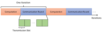
Figure 1: Timeline of the training process.

III-B Full vs. Partial Communication

Traditional convergence analyses of D-SGD focus on the objective improvement per iteration with full communication, i.e., all links are successfully used in every iteration. With our collision-free model, the communication cost per iteration is equal to the number of collision-free subsets in the full communication case. In this work, we consider the effect of partial communication, which refers to the case where not all subsets are activated in every communication round. By doing so, we can reduce the communication cost per iteration and improve the convergence speed measured by objective improvement per transmission slot.

III-C Link vs. Node Scheduling

In our work, we define the communication cost as the number of transmission slots in one communication round. With link-based scheduling, one successful information exchange over a bi-directional link requires two transmission slots. In an extreme case without concurrent transmissions, the communication cost in every round will be equal to twice the number of scheduled links in the network. On the other hand, with broadcast transmission, the communication cost will be equal to the number of scheduled broadcasting nodes. With node scheduling and broadcast transmission, we can activate more communication links with fewer transmission slots as compared to link scheduling.

Considering the aforementioned aspects, we present our proposed communication framework for D-SGD over wireless networks, namely BASS, using broadcast-based node scheduling and subgraph sampling.

IV BASS: Broadcast-Based Subgragh Sampling for Communication-Efficient D-SGD

The main idea behind BASS is that the communication cost/delay per iteration can be reduced by selecting a subgraph of the base topology to perform consensus averaging. By doing so, faster convergence can be achieved with less communication if we measure the convergence speed by the objective improvement per transmission slot.

From the mixing matrix perspective, in each iteration, the activated subgraph induces a specific structure in $\mathbf{W}(t)$, i.e., which elements in $\mathbf{W}(t)$ are non-zero. Then two questions naturally arise in our subgraph sampling design:

1. How to determine the structure (sparsity pattern) of the mixing matrix $\mathbf{W}(t)$?

2. How to optimize the elements (weights) in $\mathbf{W}(t)$ given the structure constraint?

Two possible approaches can be developed. The first one is, in every iteration $t$, we make the scheduling decision $\psi(t)\in\Psi$, following a policy $\Psi$ that can be either random or deterministic. Given the scheduling decision $\psi(t)$ and its induced subgraph $\mathcal{G}(t)$, we optimize the mixing matrix $\mathbf{W}(t)$. The second approach is, we create a family of mixing matrix candidates $\{\mathbf{W}_{r}\}_{r\in[R]}$, where each matrix $\mathbf{W}_{r}$ corresponds to one subgraph $\mathcal{G}_{r}$ activated by a specific communication decision. Then we can design a policy to select the mixing matrix in each iteration $\mathbf{W}(t)\in\{\mathbf{W}_{r}\}_{r\in[R]}$, and activate the corresponding nodes in the network.

We start with the second approach. First, nodes are divided into multiple disjoint collision-free subsets. Then, a family of candidate subgraphs are created as the union of multiple activated collision-free subsets under a given communication cost constraint. These subgraphs are randomly sampled in every iteration, and the sampling probabilities and the mixing matrices associated with these subgraphs are jointly optimized.

IV-A Step 1: Create Collision-Free Subsets

In wireless networks, information transmission and reception between a pair of nodes is always directed. To reflect the direction of communication, we view the base topology $\mathcal{G}$ as a directed graph $\mathcal{G}^{d}=(\mathcal{V},\mathcal{E}^{d})$ with bi-directional links between each pair of connected nodes.

With broadcast transmission, each broadcasting node creates a local “star” with directed links towards its neighbors. Considering the collision-free conditions, we divide the base topology into disjoint subsets of nodes $\{\mathcal{V}^{k}\}_{k\in[q]}$, where $q\leq N$ is the total number of collision-free subsets. The elements in $\mathcal{V}^{k}$ are the nodes that can transmit simultaneously without collision, i.e. $i,j\in\mathcal{V}^{k}$ if $\mathcal{N}_{i}\cap\mathcal{N}_{j}=\emptyset$. This partition satisfies $\cup_{k=1}^{q}\mathcal{V}^{k}=\mathcal{V},\mathcal{V}^{k}\cap\mathcal{V}^{l}=\emptyset,\forall k\neq l$.

Finding an optimal partition (in the sense of finding a partition with the smallest number of subsets $q$) is a combinatorial optimization problem that, in general, is NP-hard. Some heuristic algorithms can be used, such as the greedy vertex-coloring algorithm [33], that assign different colors to connected nodes. To address the constraint that two nodes cannot transmit simultaneously (be in the same subset) if they share a common neighbor, we follow a similar approach as in [31]. We apply the coloring algorithm over an auxiliary graph $\mathcal{G}^{a}=(\mathcal{V},\mathcal{E}^{a})$ where $\mathcal{E}^{a}$ includes all edges in $\mathcal{E}$ and an additional edge between each pair of nodes sharing at least one common neighbor. Then, the nodes marked with the same color will be assigned to the same subset of nodes, namely the collision-free subset. The number of subsets $q$ is equal to the number of colors found. For the base topology in Fig. 2(a), an example of dividing the base topology into multiple collision-free subsets, where each subset is marked with a different color, is given in Fig. 2(b).

Remark 1.

The graph partition obtained with the vertex-coloring algorithm is not unique. In this work, our focus is how to schedule the collision-free subsets for a given graph partition. Optimizing the graph partition can be investigated as another independent problem.

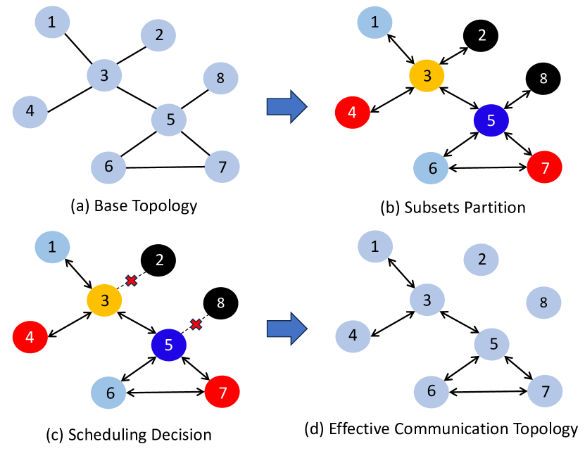
Figure 2: (a) Initial base topology. (b) Partition of collision-free subsets. (c) Scheduling multiple subsets and removing inactive nodes. (d) Effective topology with bi-directional links.

IV-B Step 2: Create Subgraph Candidates

With the collision-free protocol, the number of transmission slots in one iteration is equal to the number of scheduled collision-free subsets. For a given communication budget $\mathcal{B}$ (number of transmission slots per iteration), we can find all possible combinations of $\mathcal{B}$ collision-free subsets, obtaining a set $\mathcal{D}$ with $R=$ $q\choose\mathcal{B}$ elements, and each element $D_{r},r=1,...,R$, is a collection of $\mathcal{B}$ collision-free subsets. For example, if $\mathcal{B}=4$, using the topology in Fig. 2(a) and the collision-free subsets in Fig. 2(b), one element of $\mathcal{D}$ could be $D_{r}=\{\{1,6\},\{3\},\{4,7\},\{5\}\}$.

We further impose that when a node is not scheduled for transmission, it cannot receive neither. From the consensus averaging perspective, it means that a node will pull an update from a neighbor only when it has pushed an update to that neighbor. Then for each $D_{r}\in\mathcal{D}$, the corresponding subgraph $\mathcal{G}_{r}=\{\mathcal{V}_{r},\mathcal{E}_{r}\}$ contains the node set $\mathcal{V}_{r}=\cup_{\delta\in D_{r}}\delta$, i.e., the union of all collision-free subsets in $D_{r}$, and the link set $\mathcal{E}_{r}=\{(i,j)\in\mathcal{E}|i,j\in\mathcal{V}_{r}\}$, i.e., all the links associated to the scheduled nodes. Note that preserving only the links in the base topology that connect the nodes in $\mathcal{V}_{r}$ is equivalent to taking the base topology and disconnecting any node $i\notin V_{r}$.

Since the created subgraphs will determine the structure of the mixing matrix, the dimension of each candidate adjacency matrix should be $N\times N$. We define the adjacency matrix of the effective communication topology as

$$\mathbf{A}_{r}=\mathbf{Q}_{r}\mathbf{A}\mathbf{Q}_{r},$$ (7)

where $\mathbf{Q}_{r}=\text{diag}(n_{1},...,n_{N})$, with $n_{i}=1$ if $i\in\mathcal{V}_{r}$ and $n_{i}=0$ otherwise. For each $D_{r}$, we can create an effective communication topology and the adjacency matrix of the subgraph candidate. A visual example is given in Fig. 2(c)-(d).

IV-C Step 3: Optimize Mixing Matrices and Sampling Probabilities

With our proposed design, in every slot, a subgraph candidate $\mathcal{G}_{r}$ is randomly sampled, which corresponds to one particular scheduling decision described by $D_{r}$. The sampled subgraph in slot $t$ determines the sparsity pattern of the mixing matrix $\mathbf{W}(t)$, i.e., which elements in the matrix are non-zero. As stated in Theorem 1 in Section II-B, the spectral norm $\left\|\mathbb{E}[\mathbf{W}^{\top}(t)\mathbf{W}(t)]-\mathbf{J}\right\|_{2}$ plays a key role in the convergence speed of D-SGD. Therefore, the elements (link weights) inside each mixing matrix candidate should be determined such that $\left\|\mathbb{E}[\mathbf{W}^{\top}(t)\mathbf{W}(t)]-\mathbf{J}\right\|_{2}$ is minimized. The mixing matrix candidates and their activation probabilities can be optimized by solving:

$$\min_{\mathbf{W}_{1},...,\mathbf{W}_{R},p_{1},...,p_{R}} \left\|\sum_{r=1}^{R}p_{r}\mathbf{W}_{r}^{\top}\mathbf{W}_{r}-\mathbf{J}\right\|_{2}$$ (8)

s.t. $$\sum_{r=1}^{R}p_{r}=1,$$

$$0\leq p_{r}\leq 1,\forall r$$

$$\mathbf{W}_{r}^{\top}=\mathbf{W}_{r},\forall r$$

$$\mathbf{W}_{r}\mathbf{u}=\mathbf{u},\forall r$$

$$\mathbf{W}_{r}\in\mathcal{M}_{r},\forall r.$$

Here, $\mathcal{M}_{r}$ represents the family of mixing matrices that are consistent with the topology of subgraph candidate $\mathcal{G}_{r}$. This means that any matrix $\mathbf{M}\in\mathcal{M}_{r}$ has $M_{ij}>0$ only if $(i,j)\in\mathcal{V}_{r}$. Note that each $\mathbf{W}_{r}$ is a mixing matrix corresponding to one scheduling decision that consumes $\mathcal{B}$ transmission slots.

For a given set of mixing matrix candidates, this problem is convex with respect to the probabilities $\{p_{r}\}_{r\in[R]}$, and it can be formulated as a semidefinite programming (SDP) problem. It is also convex with respect to all $\{\mathbf{W}_{r}\}_{r\in[R]}$ for a given set of activation probabilities. The proof is given in the appendix. However, it is not jointly convex with respect to all $\{\mathbf{W}_{r}\}_{r\in[R]}$ and $\{p_{r}\}_{r\in[R]}$. For this reason, we propose to use alternating optimization to find a local minima.

IV-C1 Optimize Sampling Probabilities

For a given set of candidates of mixing matrices $\{\mathbf{W}_{r}\}_{r\in[R]}$, we optimize their activation probabilities by solving:

$$\min_{s,p_{1},...,p_{R}} s$$ (9)

s.t. $$\sum_{r=1}^{R}p_{r}\mathbf{W}_{r}^{\top}\mathbf{W}_{r}-\mathbf{J}\preccurlyeq s\mathbf{I},$$

$$\sum_{r=1}^{R}p_{r}=1,$$

$$0\leq p_{r}\leq 1,\forall r.$$

IV-C2 Optimize Each Mixing Matrix Candidate

For a given set of mixing matrix candidates $\{\mathbf{W}_{r}\}_{r\in[R]}$, and their corresponding sampling probabilities $\{p_{r}\}_{r\in[R]}$, we can optimize each candidate by solving the following problem:

$$\min_{s,\mathbf{W}_{r}} s$$ (10)

s.t. $$\begin{pmatrix}s\mathbf{I}-\mathbf{Z}_{r}&\sqrt{p_{r}}\mathbf{W}_{r}\\ \sqrt{p_{r}}\mathbf{W}_{r}&\mathbf{I}\end{pmatrix}\succcurlyeq 0,$$

$$\mathbf{W}_{r}^{\top}=\mathbf{W}_{r},$$

$$\mathbf{W}_{r}\mathbf{u}=\mathbf{u},$$

$$\mathbf{W}_{r}\in\mathcal{M}_{r}.$$

where $\mathbf{Z}_{r}=\sum_{l=1,l\neq r}^{R}p_{l}\mathbf{W}_{l}^{\top}\mathbf{W}_{l}$. We optimize one mixing matrix at a time while fixing the sampling probabilities and the other mixing matrix candidates. This can be defined as an SDP problem and solved efficiently.

The entire procedure for finding a solution to (8) is summarized in Algorithm 1, where $M$ is the number of alternating iterations. After obtaining the optimized mixing matrices $\{\mathbf{W}_{1},...,\mathbf{W}_{R}\}$ and their sampling probabilities $\{p_{1},...,p_{R}\}$, in every iteration of D-SGD, we sample one mixing matrix $\mathbf{W}(t)\in\{\mathbf{W}_{r}\}_{r\in[R]}$ with probability $\textrm{Pr}[\mathbf{W}(t)=\mathbf{W}_{r}]=p_{r}$. For a given sampling decision with mixing matrix $\mathbf{W}_{r}$, the corresponding scheduling decision can be easily determined by checking (for example, in a lookup table) which collision-free subsets have been used for creating the corresponding subgraph in $\mathbf{W}_{r}$.

Algorithm 1 Alternating Optimization Algorithm

1:

2:$\{\mathbf{W}_{r}\}_{r\in[R]},\{p_{r}\}_{r\in[R]}$, $\{\mathcal{M}_{r}\}_{r\in[R]},\text{ and }M$.

3:for $m\text{ in }[1,M]$ do

4:     for $r\text{ in }[1,R]$ do

5:         Use $\{p_{r}\}_{r\in[R]}$ to solve (10) and find $\mathbf{W}_{r}^{(m)}$

6:         Update $\{\mathbf{W}_{r}\}_{r\in[R]}$ $(\mathbf{W}_{r}\leftarrow\mathbf{W}_{r}^{(m)})$

7:         Update $\{p_{r}\}_{r\in[R]}$ solving (9) for the new $\{\mathbf{W}_{r}\}_{r\in[R]}$

8:     end for

9:end for

10:Return: $\{\mathbf{W}_{r}\}_{r\in[R]},\{p_{r}\}_{r\in[R]}$

IV-D Initial Mixing Matrix Candidates

Since problem (8) is non-convex, it may be beneficial to use more than one initialization (mixing matrix candidates and their sampling probabilities) in Algorithm 1 and choose the one the gives the smallest spectral norm. In the following, we propose two possible initialization approaches:

IV-D1 Initialization A

Suppose we have $R$ subgraph candidates, from which we can obtain the Laplacian of each subgraph as $\mathbf{L}_{r}=\mathbf{A}_{r}-\mathbf{D}_{r}$, where $\mathbf{D}_{r}$ is the degree matrix of $\mathcal{G}_{r}$. We define the mixing matrix candidates as:

$$\mathbf{W}_{r}=\mathbf{I}-\epsilon\mathbf{L}_{r}.$$ (11)

The value of $\epsilon$ needs to satisfy $\left\|\mathbb{E}[\mathbf{W}^{\top}(t)\mathbf{W}(t)]-\mathbf{J}\right\|_{2}<1$ to guarantee convergence. As stated in [24, Theorem 1], there exists an $\epsilon$ such that the previous condition is satisfied; therefore, we can find it by solving the following optimization problem:

$$\min_{s,\epsilon,\beta} s$$ (12)

s.t. $$\epsilon^{2}-\beta\leq 0,$$

$$\mathbf{I}-2\epsilon\sum_{r=1}^{R}p_{r}\mathbf{L}_{r}+\beta\sum_{r=1}^{R}p_{r}\mathbf{L}_{r}^{2}-\mathbf{J}\preccurlyeq s\mathbf{I}.$$

However, to solve (12), we need the sampling probabilities of each subgraph. As proposed in [24], we can find the sampling probabilities of the subgraph candidates by maximizing the algebraic connectivity of the expected graph. This can be done by solving the following optimization problem with concave objective function [34]:

$$\max_{p_{1},...,p_{R}} \lambda_{2}\left(\sum_{r=1}^{R}p_{r}\mathbf{L}_{r}\right)$$ (13)

s.t. $$\sum_{r=1}^{R}p_{r}=1,$$

$$0\leq p_{r}\leq 1,\forall r.$$

Since the base topology is connected, we have that $\lambda_{2}\left(\mathbf{L}\right)>0$. We also have that $\sum_{r=1}^{R}\mathbf{L}_{r}=\mathcal{H}\mathbf{L}$, where $1\leq\mathcal{H}\leq\mathcal{B}$ is a constant. If $p_{r}=\frac{1}{R}$, for $r=1,...,R$, then $\lambda_{2}\left(\sum_{r=1}^{R}p_{r}\mathbf{L}_{r}\right)=\frac{1}{R}\lambda_{2}\left(\sum_{r=1}^{R}\mathbf{L}_{r}\right)=\frac{\mathcal{H}}{R}\lambda_{2}\left(\mathbf{L}\right)>0$. This shows that the solution of (13) will not result in the case where some nodes have zero probability of being scheduled, since in this case we will have $\lambda_{2}\left(\sum_{r=1}^{R}p_{r}\mathbf{L}_{r}\right)=0$.

Once obtained the sampling probabilities as the solution to (13), we can find $\epsilon$ by solving (12), and create the set of mixing matrix candidates using (11). Algorithm 2 provides a general description of the entire training process using BASS with this initialization approach. Note that the outcome of Algorithm 1 also satisfy that no node has sampling probability equal to zero, since in this case $\left\|\mathbb{E}[\mathbf{W}^{\top}(t)\mathbf{W}(t)]-\mathbf{J}\right\|_{2}=1$, and the initialization point already satisfy that $\left\|\mathbb{E}[\mathbf{W}^{\top}(t)\mathbf{W}(t)]-\mathbf{J}\right\|_{2}<1$, which guarantee the convergence of D-SGD.

IV-D2 Initialization B

Inspired by [25], we consider an alternative initialization that might lead to smaller spectral norm. An equivalent way to represent the Laplacian is $\mathbf{L}=\mathbf{B}\mathbf{B}^{\top}$, where $\mathbf{B}\in\mathbb{R}^{N\times M}$ is the incidence matrix, and $M=|\mathcal{E}|$ is the total number of edges in the graph. The matrix $\mathbf{B}$ has elements:

$$B_{ij}=\begin{cases}1,&\text{if }s(e_{j})=i\\ -1,&\text{if }t(e_{j})=i\\ 0,&\text{otherwise}\end{cases}$$ (14)

where $s(e_{j})$ and $t(e_{j})$ are the starting and ending points respectively of the edge $e_{j}$ using an arbitrary orientation. Now, we can define the weighted Laplacian as

$$\hat{\mathbf{L}}=\mathbf{B}\text{ diag}(\bm{\alpha})\mathbf{B}^{\top},$$ (15)

where $\bm{\alpha}\in\mathbb{R}^{M}$ contains the weights of all edges in the graph. Using the weighted Laplacian, the mixing matrices are defined as $\mathbf{W}_{r}=\mathbf{I}-\hat{\mathbf{L}}_{r}$, where $\hat{\mathbf{L}}_{r}$ is the weighted Laplacian of the subgraph $\mathcal{G}_{r}$. We can optimize each weighted Laplacian matrix $\hat{\mathbf{L}}_{r}$ such that the spectral norm $||\mathbf{W}_{r}^{\top}\mathbf{W}_{r}-\mathbf{J}||_{2}$ is minimized. This is equivalent to solving the following optimization problem:

$$\min_{s,\bm{\alpha}_{r}} s$$ (16)

s.t. $$-s\mathbf{I}\preccurlyeq\mathbf{I}-\mathbf{B}_{r}\text{ diag}(\bm{\alpha}_{r})\mathbf{B}^{\top}_{r}-\mathbf{J}\preccurlyeq s\mathbf{I},$$

$$\bm{\alpha}_{r}\geq 0.$$

Note that the candidate subgraphs are not connected due to inactive nodes, thus, the minimum value of the spectral norm $||\mathbf{W}_{r}^{\top}\mathbf{W}_{r}-\mathbf{J}||_{2}$ will be $1$, and the solution to (16) is not unique. We are only interested in finding one feasible solution. The difference between this initialization and the previous one is that we do not impose that each mixing matrix has the same off-diagonal elements ($\epsilon$). Now that we have a set of mixing matrix candidates, we can solve (9) to find their sampling probabilities. This completes the initialization step in Algorithm 2.

Algorithm 2 BASS-$\mathbf{W}$-$p$ training

1:$\mathcal{G}=(\mathcal{N},\mathcal{E})$, $T$ and $\mathcal{B}$.

2:Find a partition of $\mathcal{G}$ to find the collision-free subsets as described in Section IV-A

3:Create the subgraph candidates as in Section IV-B

4:Create the initialization points as in Section IV-D

5:Optimize $\{\mathbf{W}_{r}\}_{r\in[R]}$ and $\{p_{r}\}_{r\in[R]}$ according to Algorithm 1

6:for $t\text{ in }[0,T]$ do

7:     for each user/node $i=1,\dots,N$ do in parallel

8:         $\mathbf{x}_{i}\left(t+\frac{1}{2}\right)=\mathbf{x}_{i}(t)-\eta(t)\mathbf{g}_{i}(t)$

9:     end for

10:     Sample a mixing matrix from $\mathcal{W}^{*}$ to obtain $\mathbf{W}(t)$

11:     Determine the scheduling decision $\psi(t)$ from $\mathbf{W}(t)$

12:     for each $\mathcal{S}\in\psi(t)$ do

13:         for each user/node $i\in\mathcal{S}$ do in parallel

14:              Broadcast model estimate $x_{i}\left(t+\frac{1}{2}\right)$

15:         end for

16:     end for

17:     for each user/node $i=1,\dots,N$ do in parallel

18:         $\mathbf{x}_{i}(t+1)=\sum_{j=1}^{N}{W}_{ij}(t)x_{j}\left(t+\frac{1}{2}\right)$

19:     end for

20:end for

IV-E Comparison with Existing Approaches

Some existing works consider link-based scheduling for accelerating D-SGD with limited communication costs, such as [24, 25]. However, these algorithms are not directly applicable in the wireless setting, because the partition rule does not satisfy the collision-free condition in wireless networks. In addition, even if the partition rule is modified, one link/edge will still require two transmission slots to achieve bi-directional communication. In some topologies with densely connected local parts, broadcast-based scheduling can activate many more links as compared to link-based scheduling under the same communication budget. Using a partition rule suitable for wireless networks with collision-free communication, optimizing each mixing matrix candidate and their sampling probabilities are the main novel contributions of our work. Also, we use the methods proposed in [24] to find an initial point for our mixing matrix candidates optimization; therefore, we improve the communication efficiency by further reducing the spectral norm $\left\|\mathbb{E}[\mathbf{W}^{\top}(t)\mathbf{W}(t)]-\mathbf{J}\right\|_{2}$, leading to faster convergence.

V Simplified Heuristic Design

The algorithm presented in Section IV offers a systematic approach to optimize the communication pattern and the mixing matrix design subject to a given communication cost constraint. However, this method entails solving a substantial number of optimization problems, and this number escalates rapidly with increasing network size. In this section, we propose a simpler heuristic approach to determine the scheduling decisions in every iteration and construct the mixing matrices based on these decisions.

As mentioned earlier, not all nodes are equally important in the network, and more important nodes should be scheduled more often when the communication budget is limited. After the graph partition presented in Section IV-A, we have obtained multiple collision-free subsets of nodes. Each subset $\mathcal{S}_{k}$, $\forall k\in[q]$ will be sampled/scheduled with probability $p_{\mathcal{S}_{k}}$ in every iteration. Then we have

$$\mathbb{E}[\mathbf{Q}(t)]=\text{diag}(p_{1},...,p_{N}),$$ (17)

where the diagonal elements of $\mathbf{Q}(t)$ are the scheduling decisions of each node $i\in\mathcal{N}$. Here, the scheduling probability of a node equals the scheduling probability of the subset to which it belongs, i.e. $p_{i}=p_{\mathcal{S}_{k}}$ if $i\in\mathcal{V}_{k}$. Since each subset of broadcasting nodes consumes one transmission slot, the number of transmission slots in every iteration is a random number. For a given communication budget $\mathcal{B}$, the scheduling probabilities satisfy $\sum_{l=1}^{q}p_{\mathcal{S}_{l}}=\mathcal{B}$. This quantity indicates the average number of transmission slots (average number of scheduled subsets) per iteration.

Similar to Section IV-B, from a scheduling decision (which collision-free subsets are activated), we create the adjacency matrix of the effective communication topology as $\tilde{\mathbf{A}}(t)=\mathbf{Q}(t)\mathbf{A}\mathbf{Q}(t)$. To further simplify the problem, we consider that all links have equal weight $\epsilon$ in the mixing matrix design, meaning that $\mathbf{W}(t)=\mathbf{I}-\epsilon\tilde{\mathbf{L}}(t)$, where

$$\tilde{\mathbf{L}}(t)=\text{diag}(\tilde{\mathbf{A}}(t)\mathbf{u})-\tilde{\mathbf{A}}(t).$$ (18)

The scheduling probabilities can be optimized by solving the following optimization problem:

$$\min_{p_{\mathcal{S}_{1}},...,p_{\mathcal{S}_{q}}} \left\|\mathbb{E}[\mathbf{W}^{\top}(t)\mathbf{W}(t)]-\mathbf{J}\right\|_{2}$$ (19)

s.t. $$\sum_{l=1}^{q}p_{\mathcal{S}_{l}}=\mathcal{B},$$

$$0\leq p_{\mathcal{S}_{l}}\leq 1,\forall l.$$

However, the expression for $\mathbb{E}[\mathbf{W}^{\top}(t)\mathbf{W}(t)]$ includes several nonlinear terms given by products of the probabilities, which makes the problem hard to solve. For this reason, we adopt a heuristic approach for designing the scheduling probabilities, based on the idea presented in [35]. We evaluate the importance of a node in the network by using its betweenness centrality [36]. This metric measures the number of shortest paths that pass through each node. Let $b_{i}$ represent the centrality value of node $i$. Then we define the importance value of a subset as

$$b_{\mathcal{S}_{j}}=\sum_{i=1}^{N}b_{i}\mathbf{1}_{\{i\in\mathcal{V}_{j}\}},$$ (20)

where $\mathbf{1}_{\{i\in\mathcal{V}_{j}\}}$ is an indicator function, which is equal to one if $i\in\mathcal{V}_{j}$, and zero otherwise. Finally, we choose

$$p_{\mathcal{S}_{j}}=\min\{1,\gamma b_{\mathcal{S}_{j}}\}$$ (21)

where the constant $\gamma$ is chosen such that $\sum_{i=1}^{q}p_{\mathcal{S}_{i}}=\mathcal{B}$.

Given the scheduling probabilities, the only parameter that can affect the spectral norm $\left\|\mathbb{E}[\mathbf{W}^{\top}(t)\mathbf{W}(t)]-\mathbf{J}\right\|_{2}$ is the link weight $\epsilon$. Similar to [24], we find the optimal value of $\epsilon$ by solving the following problem:

$$\min_{s,\epsilon,\beta} s$$ (22)

s.t. $$\epsilon^{2}-\beta\leq 0,$$

$$\mathbf{I}-2\epsilon\mathbb{E}\left[\tilde{\mathbf{L}}(t)\right]+\beta\left(\mathbb{E}\left[\tilde{\mathbf{L}}^{\top}(t)\tilde{\mathbf{L}}(t)\right]\right)-\mathbf{J}\preccurlyeq s\mathbf{I},$$

which is a convex problem, with $s$ and $\beta$ being auxiliary variables. If we define a function $\phi:\mathbb{R}^{2}\rightarrow\mathbb{R}$, with $\phi(i,j)=1$ if nodes $i$ and $j$ are in the same subset, and zero otherwise, we can express the $(i,j)$-th element of $\mathbb{E}\left[\tilde{\mathbf{L}}(t)\right]$ as in (23). Note that $\max\{\phi(i,j),p_{j}\}=p_{j}$ if nodes $i$ and $j$ are in different subsets and $\max\{\phi(i,j),p_{j}\}=1$ if not. Similarly, we can express the $(i,j)$-th element of $\mathbb{E}\left[\tilde{\mathbf{L}}^{\top}(t)\tilde{\mathbf{L}}(t)\right]$ as in (24)-(28). Algorithm 3 summarizes the entire process of this heuristic approach.

Algorithm 3 BASS-$\epsilon$ training

1:$\mathcal{G}=(\mathcal{N},\mathcal{E})$, $T$ and $\mathcal{B}$.

2:Find a partition of $\mathcal{G}$ to find the collision-free subsets as described in Section IV-A

3:for each subset $\mathcal{S}_{i}$ do

4:     Assign a sampling probability $p_{\mathcal{S}_{i}}$ as in (21)

5:end for

6:Solve (22) to determine $\epsilon$

7:for $t\text{ in }[0,T]$ do

8:     for each user/node $i=1,\dots,N$ do in parallel

9:         $\mathbf{x}_{i}\left(t+\frac{1}{2}\right)=\mathbf{x}_{i}(t)-\eta(t)\mathbf{g}_{i}(t)$

10:     end for

11:     Make a scheduling decision $\psi(t)$ (sample subsets)

12:     Create $\tilde{\mathbf{L}}(t)$ as in (18)

13:     Create $\mathbf{W}(t)$ as in (6)

14:     for each $\mathcal{S}\in\psi(t)$ do

15:         for each user/node $i\in\mathcal{S}$ do in parallel

16:              Broadcast model estimate $x_{i}\left(t+\frac{1}{2}\right)$

17:         end for

18:     end for

19:     for each user/node $i=1,\dots,N$ do in parallel

20:         $x_{i}(t+1)=\sum_{j=1}^{N}{W}_{ij}(t)x_{j}\left(t+\frac{1}{2}\right)$

21:     end for

22:end for

$$\left(\mathbb{E}[\tilde{\mathbf{L}}(t)]\right)_{ij}=\begin{cases}-p_{i}\max\{\phi(i,j),p_{j}\}(\mathbf{A})_{ij},&\text{if }i\neq j\\ \sum_{m=1}^{N}p_{i}\max\{\phi(i,m),p_{m}\}(\mathbf{A})_{im}(\mathbf{A})_{mi},&\text{if }i=j\end{cases}$$ (23)

$$\mathbb{E}\left[\tilde{\mathbf{L}}^{\top}(t)\tilde{\mathbf{L}}(t)\right]=\mathbb{E}\left[\text{diag}^{2}(\tilde{\mathbf{A}}\mathbf{u})\right]-\mathbb{E}\left[\text{diag}(\tilde{\mathbf{A}}\mathbf{u})\tilde{\mathbf{A}}\right]-\mathbb{E}\left[\tilde{\mathbf{A}}\text{diag}(\tilde{\mathbf{A}}\mathbf{u})\right]+\mathbb{E}\left[\tilde{\mathbf{A}}^{2}\right]$$ (24)

$$\left(\mathbb{E}\left[\text{diag}^{2}(\tilde{\mathbf{A}}\mathbf{u})\right]\right)_{ij}=\begin{cases}0,&\text{if }i\neq j\\ \sum_{m=1}^{N}\sum_{k=1}^{N}p_{i}\max\{\phi(i,m),p_{m}\}\max\{\phi(i,k),\phi(m,k),p_{k}\}(\mathbf{A})_{im}(\mathbf{A})_{ik},&\text{if }i=j\end{cases}$$ (25)

$$\left(\mathbb{E}\left[\text{diag}(\tilde{\mathbf{A}}\mathbf{u})\tilde{\mathbf{A}}\right]\right)_{ij}=\begin{cases}\sum_{m=0}^{N}p_{i}\max\{\phi(i,j),p_{j}\}\max\{\phi(i,m),\phi(j,m),p_{m}\}(\mathbf{A})_{ij}(\mathbf{A})_{im},&\text{if }i\neq j\\ 0,&\text{if }i=j\end{cases}$$ (26)

$$\left(\mathbb{E}\left[\tilde{\mathbf{A}}\text{diag}(\tilde{\mathbf{A}}\mathbf{u})\right]\right)_{ij}=\begin{cases}\sum_{m=0}^{N}p_{i}\max\{\phi(i,j),p_{j}\}\max\{\phi(i,m),\phi(j,m),p_{m}\}(\mathbf{A})_{ij}(\mathbf{A})_{jm},&\text{if }i\neq j\\ 0,&\text{if }i=j\end{cases}$$ (27)

$$\left(\mathbb{E}\left[\tilde{\mathbf{A}}^{2}\right]\right)_{ij}=\begin{cases}\sum_{m=0}^{N}p_{i}\max\{\phi(i,j),p_{j}\}\max\{\phi(i,m),\phi(j,m),p_{m}\}(\mathbf{A})_{im}(\mathbf{A})_{mj},&\text{if }i\neq j\\ \sum_{m=0}^{N}p_{i}\max\{\phi(i,m),p_{m}\}(\mathbf{A})_{im},&\text{if }i=j\end{cases}$$ (28)

V-A Discussions on Complexity and Overhead

The heuristic approach has two main advantages: the computational cost and the communication overhead. Regarding the computation complexity, this approach relies on the betweenness centrality measure of the nodes to find the sampling probabilities of the subsets, which is obtained once before the training process starts. Note that another centrality metric could be used instead. Eventually, only one optimization problem (22) needs to be solved for obtaining the mixing matrix design, and the solution is valid during the entire training process. On the other hand, the approach presented in Section IV requires to find all possible combinations of $\mathcal{B}$ subsets, and then find a good initialization point by optimizing $\{p_{r}\}_{r\in[R]}$ and $\epsilon$. Then, to find the final set of mixing matrix candidates and their activation probabilities, $2R$ optimization problems need to be solved in each step of the alternating optimization algorithm. In total, this approach requires solving $2(RM+1)$ optimization problems.

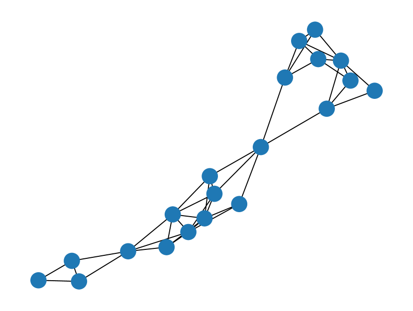
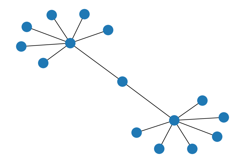
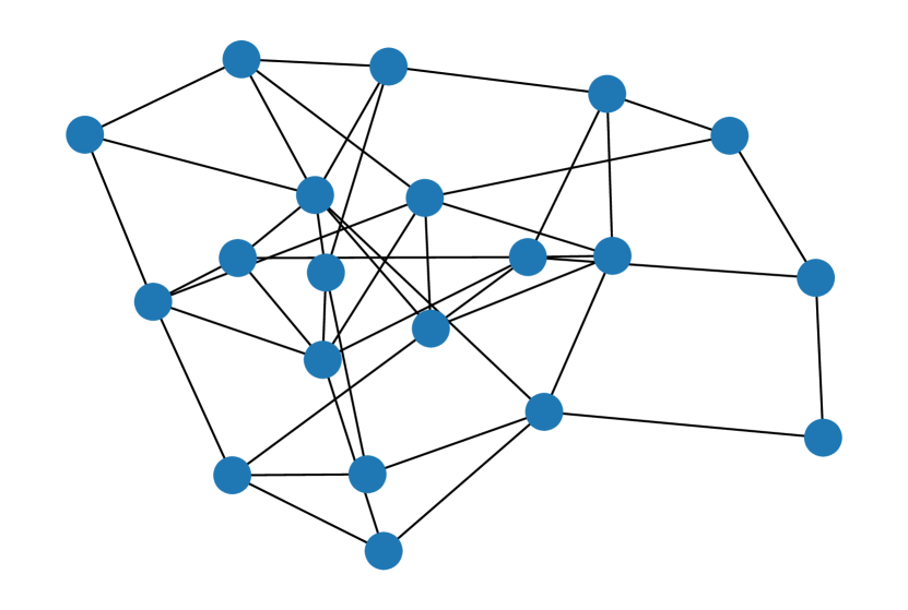
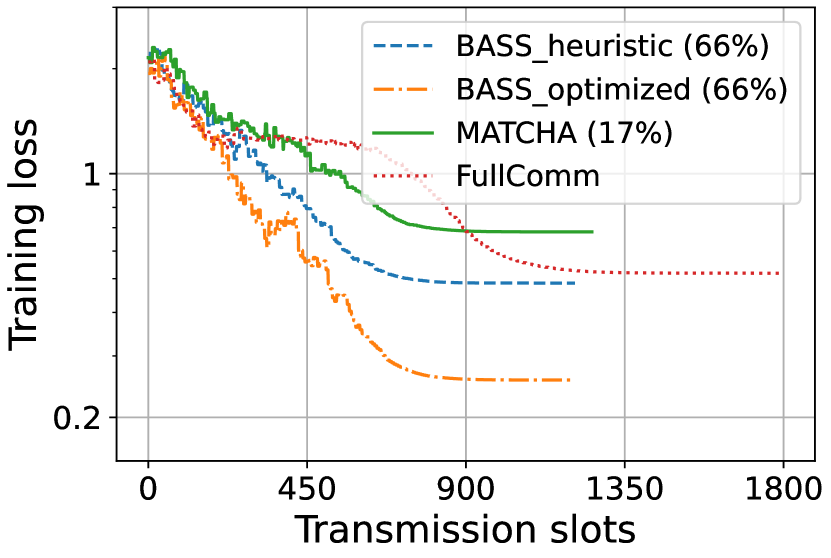
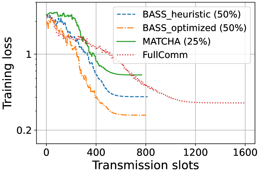
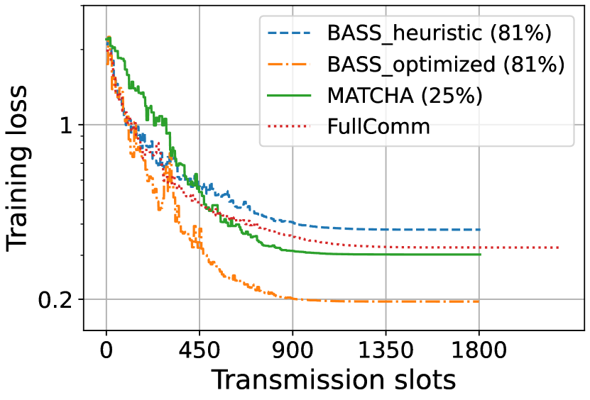
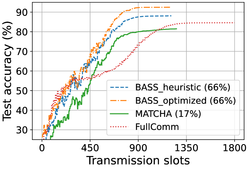
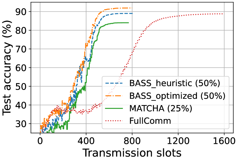
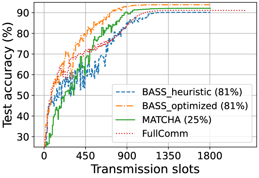
Figure 3: Performance comparison between optimized and heuristic BASS, modified MATCHA, and full communication in different topologies.

VI Numerical Experiments

In this section, we evaluate the performance of our proposed broadcast-based subgraph sampling method for D-SGD with communication cost constraints. Simulations are performed by training a multi-layer perceptron (MLP) for an image classification task. We use the MNIST dataset, which contains $60000$ images for training and $10000$ for testing. The training dataset was divided into $2N$ shards (for a total of $N$ users), and each user’s local dataset is given by $2$ randomly selected shards with no repetition. We use SparseCategoricalCrossentropy from Keras as loss function and ADAM optimizer with decaying learning rate. Each experiment runs for $200$ communication rounds (iterations). The performance of our proposed design is evaluated by showing the improvement of training loss and test accuracy with the number of transmission slots. For performance comparison, we also implement a modified version of MATCHA, and the full communication case, where all nodes are activated in every round.

VI-A Performance Evaluation of BASS

In Fig. 3, we compare the performance of optimized and heuristic BASS, modified MATCHA and full communication for different topologies. Note that full communication is a special case of BASS if all subsets are scheduled in every round. We refer to this case as “FullComm”. The percentage next to MATCHA and BASS represents the fraction of the total number of matchings and subsets that are activated on average per round, respectively. For the experiments with BASS and MATCHA, we have tested different activation percentages, and the one that gives the best performance is plotted in the figure. We observe that optimized BASS clearly outperforms modified MATCHA by a considerable margin, since the former takes advantage of broadcast transmissions, allowing us to use less transmission slots to activate more links. We can also observe clear gain in using optimized BASS over heuristic BASS. Note that heuristic BASS generally performs well for sparsely connected topologies. However, in densely connected topologies, the betweenness centrality measure is not very useful at capturing the most important nodes in the network. Another observation is that MATCHA does not always outperform the full communication case, indicating that partial communication with link scheduling is not always beneficial for improving convergence per transmission slot.

VI-B Impact of the Communication Budget

The communication budget per iteration has an impact on the performance of BASS, as shown in Fig. 4. Here, we only consider optimized BASS (referred to as BASS), and we use the second network topology in Fig. 3 as base topology. We can see that different communication budgets (the percentages in the figure) give very different results. On one hand, if the communication budget is very low (small activation percentage), the number of activated links per iteration is very low, which leads to poor information fusion/mixing. On the other hand, if the budget is very high, the communication improvement per transmission slot becomes marginal, leading to inefficient use of resources.

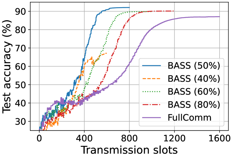
Figure 4: Impact of the communication budget in the performance of BASS.

VI-C Impact of Initial Graph Partition

With BASS, we first creates collision-free subsets through partitioning of the base topology. This partition result is not unique, and the final subgraph candidates obtained from the partitioned subsets will depend on the solution of the initial partitioning algorithm. We may improve the performance of BASS by obtaining multiple graph partitioning solutions and create all possible combinations of collision-free subsets. This will cause an increasing number of candidate subgraphs, and more optimization problems to solve to find the best communication pattern and mixing design.

A valid set of subgraph candidates is such that it contemplates the activation of all links in the base topology, otherwise convergence might not be guaranteed. One possible way of selecting a valid set of candidates is a random selection of $C$ candidates out of all possible candidates obtained by several partitioning solutions of the base topology. This will reduce the number of optimization problems to be solved. However, we should observe a decrease in performance as compared to the case when all possible candidates are considered. In this work, we obtain a valid set of candidates by considering a single partition as explained in Section IV. In Fig. 5, we observe the impact on the spectral norm $\left\|\mathbb{E}[\mathbf{W}^{\top}(t)\mathbf{W}(t)]-\mathbf{J}\right\|_{2}$ of considering different initial graph partitions using the first network topology in Fig. 3 as base topology.

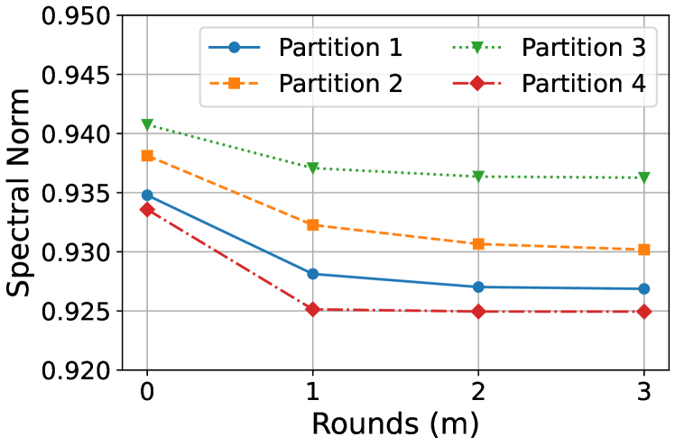
Figure 5: Spectral norm evolution per iteration $m$ of Algorithm 1, with $M=3$, for different base topology partition.

VII Conclusions and Future Directions

This work focuses on accelerating the convergence of D-SGD with broadcast-based communication design, taking into account the actual communication delay and cost per iteration. Our proposed framework, BASS, generates a family of mixing matrix candidates associated with a set of sparser subgraphs and their sampling probabilities. In each iteration of the D-SGD algorithm, one mixing matrix is randomly sampled. The corresponding subgraph indicates which set of nodes can broadcast their current models to their neighbors. Unsurprisingly, BASS outperforms existing link-based scheduling policies and plain D-SGD by a considerable margin, achieving faster convergence with fewer transmission slots.

Our findings underscore two key points: 1) Identifying and sampling subgraphs of the base topology can be exploited to customize communication dynamics and improve the error-vs-runtime tradeoff, and 2) Leveraging broadcast transmission and spatial reuse of resources can accelerate the convergence of D-SGD over wireless networks. A potential direction for future exploration involves jointly considering the impact of network connectivity and data heterogeneity in node scheduling design. Another potential extension is to optimize the communication budget allocation over time, using an adaptive or event-triggered design.

Appendix

VII-A Proof of convexity of Problem (8) for a given set of sampling probabilities

The objective function of problem (8) can be written as:

$$\left\|\mathbb{E}[\mathbf{W}^{\top}(t)\mathbf{W}(t)]-\mathbf{J}\right\|_{2}=\lambda_{\max}\left(\sum_{r=1}^{R}p_{r}\mathbf{W}_{r}^{\top}\mathbf{W}_{r}-\mathbf{J}\right)\\$$ (29)

$$= \sup_{||\mathbf{x}||_{2}=1}\mathbf{x}^{\top}\left(\sum_{r=1}^{R}p_{r}\mathbf{W}_{r}^{\top}\mathbf{W}_{r}-\mathbf{J}\right)\mathbf{x}$$ (30)

$$= \sup_{||\mathbf{x}||_{2}=1}\sum_{r=1}^{R}p_{r}\mathbf{x}^{\top}\mathbf{W}_{r}^{\top}\mathbf{W}_{r}\mathbf{x}-\mathbf{x}^{\top}\mathbf{J}\mathbf{x}$$ (31)

$$= \sup_{||\mathbf{x}||_{2}=1}\sum_{r=1}^{R}p_{r}\text{Tr}\left(\mathbf{W}_{r}\mathbf{x}\mathbf{x}^{\top}\mathbf{W}_{r}^{\top}\right)-\mathbf{x}^{\top}\mathbf{J}\mathbf{x}$$ (32)

$$= \sup_{||\mathbf{x}||_{2}=1}\sum_{r=1}^{R}p_{r}\sum_{j=1}^{N}(\mathbf{w}_{j}^{r})^{\top}\mathbf{x}\mathbf{x}^{\top}\mathbf{w}_{j}^{r}-\mathbf{x}^{\top}\mathbf{J}\mathbf{x}$$ (33)

where $\mathbf{w}_{j}^{r}$ represents the $j$-th column of the matrix $\mathbf{W}_{r}$. The function $f(\mathbf{w})=\mathbf{w}^{\top}\mathbf{x}\mathbf{x}^{\top}\mathbf{w}$ is a quadratic form with kernel $\mathbf{x}\mathbf{x}^{\top}$, which is positive semidefinite; therefore, $f(\mathbf{w})$ is convex for any fixed $\mathbf{x}$. Applying the previous reasoning to (33) and the pointwise supremum principle [37, Section 3.2.3], we conclude that the objective function is jointly convex with respect to all candidates $\{\mathbf{W}_{r}\}_{r\in[R]}$.

References

- [1] B. McMahan, E. Moore, D. Ramage, S. Hampson, and B. A. y Arcas, “Communication-efficient learning of deep networks from decentralized data,” in Artificial intelligence and statistics. PMLR, 2017, pp. 1273–1282.
- [2] B. Swenson, R. Murray, S. Kar, and H. V. Poor, “Distributed stochastic gradient descent: Nonconvexity, nonsmoothness, and convergence to local minima,” arXiv preprint arXiv:2003.02818, 2020.
- [3] X. Lian, C. Zhang, H. Zhang, C.-J. Hsieh, W. Zhang, and J. Liu, “Can decentralized algorithms outperform centralized algorithms? A case study for decentralized parallel stochastic gradient descent,” Advances in neural information processing systems, vol. 30, 2017.
- [4] R. Olfati-Saber, J. A. Fax, and R. M. Murray, “Consensus and cooperation in networked multi-agent systems,” Proceedings of the IEEE, vol. 95, no. 1, pp. 215–233, 2007.
- [5] L. Xiao and S. Boyd, “Fast linear iterations for distributed averaging,” Systems & Control Letters, vol. 53, no. 1, pp. 65–78, 2004.
- [6] A. Olshevsky and J. N. Tsitsiklis, “Convergence speed in distributed consensus and averaging,” SIAM Journal on Control and Optimization, vol. 48, no. 1, pp. 33–55, 2009.
- [7] J. Wang and G. Joshi, “Cooperative SGD: A unified framework for the design and analysis of local-update SGD algorithms,” The Journal of Machine Learning Research, vol. 22, no. 1, pp. 9709–9758, 2021.
- [8] A. Koloskova, N. Loizou, S. Boreiri, M. Jaggi, and S. Stich, “A unified theory of decentralized SGD with changing topology and local updates,” in International Conference on Machine Learning. PMLR, 2020, pp. 5381–5393.
- [9] D. Jakovetic, D. Bajovic, A. K. Sahu, and S. Kar, “Convergence rates for distributed stochastic optimization over random networks,” in IEEE Conference on Decision and Control (CDC), 2018, pp. 4238–4245.
- [10] A. Nedic and A. Ozdaglar, “Distributed subgradient methods for multi-agent optimization,” IEEE Transactions on Automatic Control, vol. 54, no. 1, pp. 48–61, 2009.
- [11] K. Scaman, F. Bach, S. Bubeck, L. Massoulié, and Y. T. Lee, “Optimal algorithms for non-smooth distributed optimization in networks,” Advances in Neural Information Processing Systems, vol. 31, 2018.
- [12] A. Nedić, A. Olshevsky, and M. G. Rabbat, “Network topology and communication-computation tradeoffs in decentralized optimization,” Proceedings of the IEEE, vol. 106, no. 5, pp. 953–976, 2018.
- [13] G. Neglia, C. Xu, D. Towsley, and G. Calbi, “Decentralized gradient methods: does topology matter?” in International Conference on Artificial Intelligence and Statistics. PMLR, 2020, pp. 2348–2358.
- [14] T. Vogels, H. Hendrikx, and M. Jaggi, “Beyond spectral gap: The role of the topology in decentralized learning,” Advances in Neural Information Processing Systems, vol. 35, pp. 15 039–15 050, 2022.
- [15] A. Koloskova, S. Stich, and M. Jaggi, “Decentralized stochastic optimization and gossip algorithms with compressed communication,” in International Conference on Machine Learning. PMLR, 2019, pp. 3478–3487.
- [16] A. I. Rikos, W. Jiang, T. Charalambous, and K. H. Johansson, “Distributed optimization via gradient descent with event-triggered zooming over quantized communication,” in IEEE Conference on Decision and Control (CDC), 2023, pp. 6321–6327.
- [17] H. Ye, L. Liang, and G. Y. Li, “Decentralized federated learning with unreliable communications,” IEEE Journal of Selected Topics in Signal Processing, 2022.
- [18] Z. Jiang, G. Yu, Y. Cai, and Y. Jiang, “Decentralized edge learning via unreliable device-to-device communications,” IEEE Transactions on Wireless Communications, vol. 21, no. 11, pp. 9041–9055, 2022.
- [19] N. Lee, H. Shan, M. Song, Y. Zhou, Z. Zhao, X. Li, and Z. Zhang, “Decentralized federated learning under communication delays,” in International Conference on Sensing, Communication, and Networking (SECON Workshops). IEEE, 2022, pp. 37–42.
- [20] X. Wu, C. Liu, S. Magnusson, and M. Johansson, “Asynchronous distributed optimization with delay-free parameters,” arXiv preprint arXiv:2312.06508, 2023.
- [21] Y. Lu and C. De Sa, “Moniqua: Modulo quantized communication in decentralized SGD,” in International Conference on Machine Learning. PMLR, 2020, pp. 6415–6425.
- [22] H. Tang, S. Gan, C. Zhang, T. Zhang, and J. Liu, “Communication compression for decentralized training,” Advances in Neural Information Processing Systems, vol. 31, 2018.
- [23] D. Alistarh, D. Grubic, J. Li, R. Tomioka, and M. Vojnovic, “QSGD: Communication-efficient SGD via gradient quantization and encoding,” Advances in neural information processing systems, vol. 30, 2017.
- [24] J. Wang, A. K. Sahu, G. Joshi, and S. Kar, “MATCHA: A matching-based link scheduling strategy to speed up distributed optimization,” IEEE Transactions on Signal Processing, vol. 70, pp. 5208–5221, 2022.
- [25] C.-C. Chiu, X. Zhang, T. He, S. Wang, and A. Swami, “Laplacian matrix sampling for communication-efficient decentralized learning,” IEEE Journal on Selected Areas in Communications, vol. 41, no. 4, pp. 887–901, 2023.
- [26] S. Liu, G. Yu, D. Wen, X. Chen, M. Bennis, and H. Chen, “Communication and energy efficient decentralized learning over D2D networks,” IEEE Transactions on Wireless Communications, 2023.
- [27] N. Singh, D. Data, J. George, and S. Diggavi, “Squarm-SGD: Communication-efficient momentum sgd for decentralized optimization,” IEEE Journal on Selected Areas in Information Theory, vol. 2, no. 3, pp. 954–969, 2021.
- [28] A. Nedić and A. Olshevsky, “Distributed optimization over time-varying directed graphs,” IEEE Transactions on Automatic Control, vol. 60, no. 3, pp. 601–615, 2014.
- [29] A. Nedic, “Asynchronous broadcast-based convex optimization over a network,” IEEE Transactions on Automatic Control, vol. 56, no. 6, pp. 1337–1351, 2010.
- [30] R. Xin, S. Pu, A. Nedić, and U. A. Khan, “A general framework for decentralized optimization with first-order methods,” Proceedings of the IEEE, vol. 108, no. 11, pp. 1869–1889, 2020.
- [31] H. Xing, O. Simeone, and S. Bi, “Federated learning over wireless device-to-device networks: Algorithms and convergence analysis,” IEEE Journal on Selected Areas in Communications, vol. 39, no. 12, pp. 3723–3741, 2021.
- [32] Z. Chen, M. Dahl, and E. G. Larsson, “Decentralized learning over wireless networks: The effect of broadcast with random access,” in IEEE International Workshop on Signal Processing Advances in Wireless Communications (SPAWC), 2023, pp. 316–320.
- [33] B. Bollobás, Modern graph theory. Springer Science & Business Media, 1998, vol. 184.
- [34] S. Boyd, “Convex optimization of graph laplacian eigenvalues,” in Proceedings of the international congress of mathematicians, vol. 3, no. 1-3. Citeseer, 2006, pp. 1311–1319.
- [35] D. P. Herrera, Z. Chen, and E. G. Larsson, “Distributed consensus in wireless networks with probabilistic broadcast scheduling,” IEEE Signal Processing Letters, vol. 30, pp. 41–45, 2023.
- [36] V. Latora, V. Nicosia, and G. Russo, Complex networks: principles, methods and applications. Cambridge University Press, 2017.
- [37] S. P. Boyd and L. Vandenberghe, Convex optimization. Cambridge university press, 2004.