Fast System Level Synthesis:
Robust Model Predictive Control using Riccati Recursions

Abstract

System level synthesis (SLS) enables improved robust MPC formulations by allowing for joint optimization of the nominal trajectory and controller. This paper introduces a tailored algorithm for solving the corresponding disturbance feedback optimization problem. The proposed algorithm builds on a recently proposed joint optimization scheme and iterates between optimizing the controller and the nominal trajectory while converging q-linearly to an optimal solution. We show that the controller optimization can be solved through Riccati recursions leading to a horizon-length, state, and input scalability of $\mathcal{O}(N^{2}(n_{\mathrm{x}}^{3}+n_{\mathrm{u}}^{3}))$ for each iterate. On a numerical example, the proposed algorithm exhibits computational speedups of order $10$ to $10^{3}$ compared to general-purpose commercial solvers.

1 Introduction

The ability to plan safe trajectories in real-time, despite model mismatch and external disturbances, is a key enabler for high-performance control of autonomous systems (Majumdar and Tedrake, 2017; Schulman et al., 2014). iLQR (Li and Todorov, 2004; Giftthaler et al., 2018) methods have shown great practical benefits (Neunert et al., 2016; Howell et al., 2019) by producing a feedback controller based on the optimal nominal trajectory. However, robust stability and robust constraint satisfaction are generally only addressed heuristically (Manchester and Kuindersma, 2017).

Model predictive control (MPC) (Rawlings et al., 2017) has emerged as a key technology for control subject to (safety) constraints. Real-time feasibility of MPC, even in fast-sampled systems, is largely due to advancements in numerical optimization (Frison, 2016; Domahidi et al., 2012). These tailored algorithms exploit the stage-wise structure of the nominal trajectory optimization problem, utilizing, e.g., efficient Riccati recursions. Robust MPC approaches can account for model mismatch and external disturbances by propagating them over the prediction horizon. While few robust MPC approaches optimize a feedback policy (Scokaert and Mayne, 1998; Villanueva et al., 2017; Messerer and Diehl, 2021; Kim et al., 2022), most robust MPC designs use an offline-fixed controller (Mayne et al., 2005; Köhler et al., 2020; Zanelli et al., 2021) for computational efficiency.

Disturbance feedback (Goulart et al., 2006; Ben-Tal et al., 2004) overcomes this limitation by using a convex controller parametrization. Building on this parametrization, system level synthesis (SLS) (Anderson et al., 2019; Tseng et al., 2020; Li et al., 2023) facilitates the consideration of constraints on the closed-loop response. SLS has also been proposed within an MPC formulation (Sieber et al., 2021; Chen et al., 2022; Leeman et al., 2023a, b). However, the large number of decision variables in SLS poses a major obstacle for real-time implementation.

Figure 1: Illustration how the robust MPC problem (7) is solved by alternating between a nominal trajectory optimization problem with tightened constraints and the computation of optimal feedback gains $K^{k,j}$ using Riccati recursions.

Asynchronous updates (Sieber et al., 2023) or GPU parallelization (Alonso and Tseng, 2022) can reduce the computational time. Goulart et al. (2008) derived a structure-exploiting solver for disturbance feedback optimization, reducing the scalability of a naive interior-point method implementation from $\mathcal{O}(N^{6})$ to $\mathcal{O}(N^{3})$ per iteration. In this work, we leverage results in numerical optimization (Wright et al., 1999; Messerer and Diehl, 2021) to propose a customized optimization solver for SLS with $\mathcal{O}(N^{2})$ scalability, significantly improving the computation times.

Contribution

Our key contribution is an efficient solution to robust MPC problems, that are based on an SLS formulation. This is achieved through iterative optimization of the nominal trajectory and the controller, as inspired by Messerer and Diehl (2021) and illustrated in Fig. 1.

The proposed algorithm has the following properties:

• It converges q-linearly to an optimal solution of a tightened robust MPC problem.

• Each controller optimization is solved with efficient Riccati recursions with a combined scalability of $\mathcal{O}(N^{2}(n_{\mathrm{x}}^{3}+n_{\mathrm{u}}^{3}))$.

• The proposed algorithm also allows for parallelization, leading to a scalability of $\mathcal{O}(N(n_{\mathrm{x}}^{3}+n_{\mathrm{u}}^{3}))$.

We showcase the numerical properties of our solver for a range of state dimensions and horizon lengths in comparison to the commercial general-purpose solvers Gurobi Optimization (2023), and Mosek ApS (2019) (Section 2).

Notation

We denote stacked vectors or matrices by $(a,\ldots,b)=[a^{\top},\ldots,b^{\top}]^{\top}$. The matrix ${I}$ denotes the identity with its dimensions either inferred from the context or indicated by the subscript, i.e., ${I}_{n_{\mathrm{x}}}\in\mathbb{R}^{n_{\mathrm{x}}\times n_{\mathrm{x}}}$, the matrix $\mathbf{0}_{n,m}\in\mathbb{R}^{n\times m}$ has all its elements zeros, and the vector $\bm{1}_{n}\in\mathbb{R}^{n}$ has all its elements one. For a sequence of matrices $\bm{\Phi}_{\mathrm{u}}^{k,j}$, we define $\bm{\Phi}_{\mathrm{u}}^{0:k,j}:=(\bm{\Phi}_{\mathrm{u}}^{0,j},\ldots,\bm{\Phi}_{\mathrm{u}}^{k,j})$. Similarly, for a sequence of vectors $x_{k}$, we define $\mathbf{x}:=(x_{0},\ldots,x_{k})$. We define the Frobenius norm of a matrix $A\in\mathbb{R}^{m\times n}$, as $\|A\|_{\mathcal{F}}=\text{Trace}(A^{\top}A)$. For a non-negative vector $x\in\mathbb{R}^{n}$, the square root $\sqrt{x}$ is to be understood elementwise. Besides, $0\leq x\perp y\leq 0$ is the shorthand notation for the three conditions $x_{i}\cdot y_{i}=0,$$~{}x_{i}\geq 0,~{}y_{i}\leq 0,~{}i=1,\ldots,n$. The set of positive definite matrices is denoted by $\mathbb{S}_{++}^{n}$. We denote the unit ball, centered at the origin, $\mathcal{E}_{n}:=\left\{x\in\mathbb{R}^{n},x^{\top}x\leq 1\right\}$. For a vector valued function $f:\mathbb{R}^{n}\rightarrow\mathbb{R}^{q}$, we denote by $\nabla\phi(x)\in\mathbb{R}^{n\times q}$ the transposed Jacobian $\frac{\partial\phi(x)}{\partial x}$.

2 Problem setup & System Level Synthesis

We consider the following uncertain linear time-varying (LTV) system:

$$x_{k+1}=A_{k}x_{k}+B_{k}u_{k}+E_{k}w_{k},~{}x_{0}=\bar{x}_{0},$$ (1)

with state $x_{k}\in\mathbb{R}^{n_{\mathrm{x}}}$, input $u_{k}\in\mathbb{R}^{n_{\mathrm{u}}}$ and disturbance $w_{k}\in\mathcal{E}_{n_{\mathrm{x}}}$ which lies in a unit ball, and $E_{k}\in\mathbb{S}_{++}^{n_{\mathrm{x}}}$. The initial conditions are given by $\bar{x}_{0}\in\mathbb{R}^{n_{\mathrm{x}}}$. The system is subject to the affine constraints,

$$g_{ki}^{\top}(x_{k},u_{k})+b_{ki}\leq 0,~{}\forall i=1,\ldots,n_{\mathrm{c}},$$ (2a)

$$~{}g_{\mathrm{f}i}^{\top}x_{N}+b_{\mathrm{f}i}\leq 0,~{}\forall i=1,\ldots,n_{\mathrm{f}},$$ (2b)

for $k=0,\ldots,N-1$ with $g_{ki}\in\mathbb{R}^{n_{\mathrm{x}}+n_{\mathrm{u}}}$, and $g_{\mathrm{f}i}\in\mathbb{R}^{n_{\mathrm{x}}}$.

We consider the problem of designing an optimal controller with the following cost

$$J(\mathbf{x},\mathbf{u})=\sum_{k=0}^{N-1}{x}_{k}^{\top}Q{x}_{k}+{u}_{k}^{\top}R{u}_{k}+{x}_{N}^{\top}P{x}_{N},$$ (3)

with $Q\in\mathbb{S}_{++}^{n_{\mathrm{x}}}$, $R\in\mathbb{S}_{++}^{n_{\mathrm{u}}}$, $P\in\mathbb{S}_{++}^{n_{\mathrm{x}}}$.

We optimize over disturbance feedback

$$u_{k}=v_{k}+\sum_{j=0}^{k-1}\bm{\Phi}_{\mathrm{u}}^{k,j}w_{j},$$ (4)

with nominal input $v_{k}\in\mathbb{R}^{n_{\mathrm{u}}}$, i.e., we assign a distinct disturbance feedback matrix $\bm{\Phi}_{\mathrm{u}}^{k,j}\in\mathbb{R}^{n_{\mathrm{u}}\times n_{\mathrm{x}}}$ for each disturbance $w_{j}$ and control $u_{k}$ with $k>j$. As common in SLS, the resulting state sequence can be expressed as

$$x_{k}=z_{k}+\sum_{j=0}^{k-1}\bm{\Phi}_{\mathrm{x}}^{k,j}w_{j},~{}z_{0}=x_{0},$$ (5)

where $z_{k}$ is the corresponding nominal state and the corresponding closed-loop response $\bm{\Phi}_{\mathrm{x}}^{k,j}\in\mathbb{R}^{n_{\mathrm{x}}\times n_{\mathrm{x}}}$ denotes the influence of the disturbance $w_{j}$ on the state $x_{k}$. Starting with $\bm{\Phi}_{\mathrm{x}}^{j+1,j}=E_{j}$, the propagation of the disturbance, commonly used in SLS, is governed by

$$\bm{\Phi}_{\mathrm{x}}^{k+1,j}=A_{k}\bm{\Phi}_{\mathrm{x}}^{k,j}+B_{k}\bm{\Phi}_{\mathrm{u}}^{k,j},$$ (6)

$j=0,\ldots,N-1$, $k=j+1,\ldots,N-1$. Combining the disturbance propagation for each time step (6), we formulate the robust optimal control problem via SLS as a second-order cone program (SOCP),

$$\min_{\begin{subarray}{c}{\bm{\Phi}_{\mathrm{x}}},{\bm{\Phi}_{\mathrm{u}}},\\ \mathbf{z},\mathbf{v}\end{subarray}} J(\mathbf{z},\mathbf{v})+\tilde{H}_{0}(\mathbf{\Phi}),$$ (7a)

s.t. $${z}_{k+1}=A_{k}z_{k}+B_{k}v_{k},~{}{z}_{0}=\bar{x}_{0},$$ (7b)

$$k=0,\ldots,N-1,$$

$$\bm{\Phi}_{\mathrm{x}}^{k+1,j}=A_{k}\bm{\Phi}_{\mathrm{x}}^{k,j}+B_{k}\bm{\Phi}_{\mathrm{u}}^{k,j},~{}\bm{\Phi}_{\mathrm{x}}^{j+1,j}=E_{j},$$ (7c)

$$j=0,\ldots,N-1,~{}k=j+1,\ldots,N-1,$$

$$\sum_{j=0}^{k-1}\left\|g_{ki}^{\top}\mathbf{\Phi}^{k,j}\right\|_{2}+g_{ki}^{\top}({z}_{k},{v}_{k})+b_{ki}\leq 0,$$ (7d)

$$i=1,\ldots,n_{c},~{}k=0,\ldots,N-1,$$

$$\sum_{j=0}^{N-1}\left\|g_{\mathrm{f}i}^{\top}\mathbf{\Phi}^{N,j}\right\|_{2}+g_{\mathrm{f}i}^{\top}{z}_{k}+b_{\mathrm{f}i}\leq 0,$$ (7e)

$$i=1,\ldots,n_{\mathrm{f}},$$

with $\mathbf{\Phi}^{k,j}:=(\bm{\Phi}_{\mathrm{x}}^{k,j},\bm{\Phi}_{\mathrm{u}}^{k,j})$, $\mathbf{\Phi}^{N,j}:=\bm{\Phi}_{\mathrm{x}}^{N,j}$. Compared to disturbance feedback (Goulart et al., 2006), the specificity of this SLS formulation is to consider explicitly the disturbance propagation (7c).

Conditions (7b) implement nominal dynamics, while the tightened constraints (7d), (7e) ensure the constraints (2) are satisfied robustly (see Proposition 1). The cost (7a) includes

$$\tilde{H}_{0}(\mathbf{\Phi}):=$$ (8)

$$\sum_{j=0}^{N-1}\left(\|P^{\frac{1}{2}}\bm{\Phi}_{\mathrm{x}}^{N,j}\|_{\mathcal{F}}^{2}+\sum_{k=j}^{N-1}\left(\|Q^{\frac{1}{2}}\bm{\Phi}_{\mathrm{x}}^{k,j}\|_{\mathcal{F}}^{2}+\|R^{\frac{1}{2}}\bm{\Phi}_{\mathrm{u}}^{k,j}\|_{\mathcal{F}}^{2}\right)\right),$$

with the high-dimensional variable $\mathbf{\Phi}$ collecting all $\bm{\Phi}_{\mathrm{x}}$, and $\bm{\Phi}_{\mathrm{u}}$.

Proposition 1

(Goulart et al., 2006) System (1) in closed-loop with (4) satisfies constraints (2) for all disturbances $w=(w_{0},\dots,w_{N-1})\in\mathcal{E}_{n_{\mathrm{x}}}\times\cdots\times\mathcal{E}_{n_{\mathrm{x}}}$ if and only if $(\mathbf{z},\mathbf{v})$ and $(\bm{\Phi}_{\mathrm{x}},\bm{\Phi}_{\mathrm{u}})$ satisfy the constraints in (7).

Remark 2.1

Under suitable terminal ingredients $P$, $g_{\mathrm{f}i}$, $b_{\mathrm{f}i}$, the optimization problem (7), used in a receding-horizon fashion, is recursively feasible and ensures a stable closed-loop system, see, e.g., (Goulart et al., 2006).

Remark 2.2

In the SLS literature, the constraint (7c) is often written equivalently in its matrix form:

$$\left[\mathbf{I}-\mathbf{Z}{\mathbf{A}},~{}-\mathbf{Z}{\mathbf{B}}\right]\begin{bmatrix}\bm{\Phi}_{\mathrm{x}}\\ \bm{\Phi}_{\mathrm{u}}\\ \end{bmatrix}=\mathbf{E}.$$ (9)

see, e.g., (Anderson et al., 2019, Eq.(2.7)).

In the following, we exploit the structural similarity between the optimization problem (7), and the optimization problem efficiently solved in (Messerer and Diehl, 2021). In contrast to standard tube-based MPC, the SLS-based formulation (10) is not conservative (Proposition 1). However, this approach results in a large number of decision variables, e.g., $\frac{N\cdot(N-1)}{2}n_{\mathrm{x}}n_{\mathrm{u}}$ for $\bm{\Phi}_{\mathrm{u}}$. This paper proposes a structure-exploiting solver for the optimization problem (7).

3 Efficient algorithm for SLS

In this section, we show how to efficiently solve the SLS-based problem (7). The Karush–Kuhn–Tucker (KKT) conditions (Wright et al., 1999) of (7) are decomposed into two subsets. The proposed algorithm iteratively solves each subset, corresponding to the nominal trajectory optimization and controller optimization employing efficient Riccati recursions (cf. Fig.1).

3.1 SLS and its KKT conditions

We first write the SLS optimization problem compactly and present its KKT conditions. We summarize the SLS problem (7) as

$$\min_{y,\mathbf{\Phi},\beta}\quad J(y)+\tilde{H}_{0}(\mathbf{\Phi}),$$ (10a)

s.t. $$f(y)=0,$$ (10b)

$$D(\mathbf{\Phi})=0,$$ (10c)

$$h(y)+h_{\mathrm{bo}}(\beta)\leq 0,$$ (10d)

$$\tilde{H}(\mathbf{\Phi})-\beta=0,$$ (10e)

where $y=(\mathbf{z},\mathbf{v})\in\mathbb{R}^{{n_{\mathrm{y}}}}$ contains the variables associated with the nominal trajectory, the constraint (10b) encodes the nominal dynamics (7b), and the constraint (10c) encodes the disturbance propagation (7c). The tightened constraints (7d)-(7e) are split into two constraints: Inequality (10d) captures the nominal constraints $h(y)$ with a constraint tightening $h_{\textrm{bo}}(\beta)$ and (10e) captures the nonlinear relation between $\beta$ and the disturbance propagation $\mathbf{\Phi}$. In (10d), and (10e), the tightenings are defined based on

$$h_{\mathrm{bo}}^{k}(\beta_{k}):=\sum_{j=0}^{k-1}\sqrt{\beta_{k}^{j}+\epsilon_{\beta}},~{}h_{\mathrm{bo}}^{0}:=0_{n_{\mathrm{c}}},$$ (11a)

$$\beta_{k}^{j}=\tilde{H}^{k,j}(\mathbf{\Phi}):=(\|g_{k1}^{\top}\mathbf{\Phi}^{k,j}\|_{2}^{2},\ldots,\|g_{kn_{\mathrm{c}}}^{\top}\mathbf{\Phi}^{k,j}\|_{2}^{2}),$$ (11b)

with $\beta_{k}^{j}\in\mathbb{R}^{n_{\mathrm{c}}}$, similar for $\beta_{N}$, $\beta_{k}:=(\beta_{k}^{0},\dots,\beta_{k}^{k-1})$, $\beta:=(\beta_{1},\dots,\beta_{N})$, and $h_{\mathrm{bo}}(\beta):=(0_{n_{\mathrm{c}}},h_{\mathrm{bo}}^{1}(\beta_{1}),\dots,h_{\mathrm{bo}}^{N}(\beta_{N}))$. We note that the tightenings (11a) are equivalent to those used in (7) if $\epsilon_{\beta}=0$. However, in the following, we use a fixed $\epsilon_{\beta}>0$ to circumvent points of non-differentiability.

To derive an efficient algorithm for solving the SLS-based problem (10), we first condense the disturbance propagation (10c) within the tightening definition (10e). This is achieved by recursively substituting all $\bm{\Phi}_{\mathrm{x}}^{k,j}$ with a corresponding function of the gains $\bm{\Phi}_{\mathrm{u}}^{k,j}$ and disturbance gains $E_{j}$ using (6). After substitution, we obtain the equivalent, more compact, optimization problem

$$\min_{y,M,\beta}\quad J(y)+H_{0}(M),$$ (12a)

s.t. $$f(y)=0,$$ (12b)

$$h(y)+h_{\mathrm{bo}}(\beta)\leq 0,$$ (12c)

$$H(M)-\beta=0,$$ (12d)

where $M$ collects all the disturbance feedback controller gains $\bm{\Phi}_{\mathrm{u}}^{k,j}$ in a vector, and $H$ is a composition function condensing the disturbance propagation (10c), such that $H(M)=\tilde{H}(\mathbf{\Phi})$ and $H_{0}(M)=\tilde{H}_{0}(\mathbf{\Phi})$, for any $\mathbf{\Phi}$ with $D(\mathbf{\Phi})=0$. The Lagrangian of (12) is given by

$$\mathcal{L}(y,\beta,M,\lambda,\mu,\eta)$$ (13)

$$=J(y)+H_{0}(M)+\lambda^{\top}f(y)+\mu^{\top}(h(y)+h_{\mathrm{bo}}(\beta))$$

$$\quad+\eta^{\top}(H(M)-\beta),$$

with the dual variables $\lambda$, $\mu$, and $\eta$. The KKT conditions of (12) are given by

$$\nabla J(y)+\nabla f(y)\lambda+\nabla h(y)\mu =0,$$ (14a)

$$\nabla h_{\mathrm{bo}}(\beta)\mu-\eta =0,$$ (14b)

$$\nabla H_{0}(M)+\nabla H(M)\eta =0,$$ (14c)

$$f(y) =0,$$ (14d)

$$0\leq\mu\perp h(y)+h_{\mathrm{bo}}(\beta) \leq 0,$$ (14e)

$$H(M)-\beta =0,$$ (14f)

where $\perp$ denotes a complementarity condition. The next section shows how to exploit the structure in (14) to efficiently solve the SLS-based problem.

3.2 Iterative trajectory and controller optimization

In the following, we derive the proposed algorithm and we outline its convergence properties. The main idea of the proposed algorithm is to partition the KKT conditions (14) into two subsets solved alternatingly: one subset corresponding to the nominal trajectory optimization and the other to controller optimization.

In particular, the subset of necessary conditions (14a), (14b), (14d), (14e) with fixed $\bar{\beta}$, corresponds to a nominal trajectory optimization,

$$\nabla J(y)+\nabla f(y)\lambda+\nabla h(y)\mu =0,$$ (15a)

$$f(y) =0,$$ (15b)

$$0\leq\mu\perp h(y)+h_{\mathrm{bo}}(\bar{\beta}) \leq 0,$$ (15c)

$$\nabla h_{\mathrm{bo}}(\bar{\beta})\mu-\eta =0.~{}$$ (15d)

Conditions (15) yield an optimal dual $\bar{\eta}$. This optimal dual is fixed to solve the remaining necessary conditions (14c), (14f), corresponding to the controller optimization

$$\nabla H_{0}(M)+\nabla H(M)\bar{\eta} =0,$$ (16a)

$$H(M)-\beta =0.$$ (16b)

The solution to (16) yields a new update for $\beta$, used in (15). A similar iterative scheme was derived in (Messerer and Diehl, 2021) for a different robust optimal control problem, with each iteration refining the trajectory based on the computed feedback, while ensuring convergence towards an optimal solution (see Proposition 2). Next, we detail how the decomposition in subsets (15) and (16) enables a fast solution.

3.3 Algorithm

The solution of (15) can be obtained by solving a nominal trajectory optimization problem,

$$\min_{\mathbf{z},\mathbf{v}}\quad J(\mathbf{z},\mathbf{v}),$$ (17a)

s.t. $${z}_{k+1}=A_{k}z_{k}+B_{k}v_{k},~{}{z}_{0}=\bar{x}_{0},$$ (17b)

$$h_{\mathrm{bo}}^{k}(\bar{\beta}_{k})+G_{k}({z}_{k},{v}_{k})+b_{k}\leq 0,$$ (17c)

$$k=0,\ldots,N-1,$$

$$h_{\mathrm{bo}}^{N}(\bar{\beta}_{N})+G_{\mathrm{f}}{z}_{N}+b_{\mathrm{f}}\leq 0,$$ (17d)

with the tightenings based on a fixed $\bar{\beta}$, and where $G_{k}$ and $G_{\mathrm{f}}$ collect, respectively, all $g_{ki}^{\top}$ and $g_{\mathrm{f}i}^{\top}$ in a matrix. Importantly, the stage-wise optimal control structure of the quadratic program (QP) (17) enables the use of tailored QP solvers (Kouzoupis et al., 2018) including efficient Riccati recursions (Steinbach, 1995; Rao et al., 1998; Frison and Diehl, 2020).

Note 3.1

I am not sure if I can read the text linked to $\bar{\beta}$. The optimal value of $\eta$ is then obtained by evaluating (15d), i.e.,

$$\eta_{k}^{j}=\frac{\mu_{k}}{2\sqrt{\bar{\beta}_{k}^{j}}}~{}j=0,\ldots,N-1,~{}k=j,\ldots,N-1,$$ (18)

where $\eta_{k}^{j}\in\mathbb{R}^{n_{c}}$ are the dual variables that correspond to each $\beta_{k}^{j}$ for the equality constraint (14f), and $\mu_{k}\in\mathbb{R}^{n_{c}}$ are the dual variables that correspond, at time step $k$, to the tightened constraints (14e).

Then, to efficiently solve (16) given a fixed $\bar{\eta}$, we notice that the stationarity condition (16a) is linear in $M$ and has a unique solution. This condition can be solved with efficient Riccati recursions, as detailed in Section 3.4. Finally, the updated tightenings are obtained by evaluating (16b), which corresponds to the forward simulation given by (7c), and (11). Algorithm 1 summarizes the steps previously outlined.

Algorithm 1 fast-SLS

$Q$, $R$, $P$, $A_{k}$, $B_{k}$, $E_{k}$, $G_{ki}$, $b_{ki}$ $G_{\mathrm{f}}$, $b_{\mathrm{f}}$

$\beta,\bar{x}_{0}\leftarrow\text{Initialize tightening (e.g., $\epsilon_{\beta}$), current state}$

while KKT $\eqref{eq:KKT}$ not satisfied do

     $\mathbf{z},\mathbf{v},\mu\leftarrow\text{Optimize nominal trajectory}$ $\triangleright$ (17)

     $\eta,C_{k}^{j}\leftarrow\text{Update dual, and cost}$$\triangleright$ (18), (21)

     $\bm{\Phi}_{\mathrm{x}},\bm{\Phi}_{\mathrm{u}}\leftarrow\text{Optimize controller}$ $\triangleright$ (23)

     $\beta\leftarrow~{}\text{Update tightening}$$\triangleright$ (7c), (11)

end while

Output: $\mathbf{z}^{\star},~{}\mathbf{v}^{\star},~{}\bm{\Phi}_{\mathrm{x}}^{\star},~{}\bm{\Phi}_{\mathrm{u}}^{\star}$ satisfy (10)

Proposition 2

Denote by $s^{\star}:=(y^{\star},M^{\star},\beta^{\star})$ the unique optimal solution of (10) or (12) and assume standard regularity conditions hold at $s^{\star}$, i.e., linear independence constraint qualification (LICQ), the second order sufficient condition (SOSC), and strict complementarity. Then, the sequences $\{s_{i}\}_{i=0}^{\infty}$, generated by Algorithm 2, converge to $s^{\star}$ if $\sigma=\max_{k}\|E_{k}\|$ is sufficiently small and if $\beta$ and the corresponding $y$ are initialized sufficiently close to $s^{\star}$. The convergence rate is q-linear in the nominal trajectory variables $y$ and r-linear in the controller variables $\mathbf{\Phi}$, and $\beta$.

The proof is analogous to (Messerer and Diehl, 2021, Thm. 10). Specifically, by fixing $\bar{\beta}$ in (15), we implicitly neglect the corresponding Jacobians with respect to the remaining variables. As in (Messerer and Diehl, 2021), the magnitude of the neglected Jacobians is proportional to $\sigma$. Hence, for $\sigma$ small enough, we obtain linear convergence, whereas quadratic convergence is not possible because of the neglected gradients. Notably, Messerer and Diehl (2021) use a gradient-correction to ensure convergence to a KKT point. However, this is not needed for the convex problem (10) and Algorithm 1 converges to the global minimizer $s^{\star}$. $\hfill\square$

Note 3.2

There is a comment in the margin that I am not able to read, I guess because of the scanner.

Remark 3.3

Without inequality constraints, a single trajectory and controller optimization results in an optimal solution.

Remark 3.4

As stopping criterion, we compare the norm of the difference between two consecutive primal solutions to a specified threshold, denoted as $\epsilon_{m}$.

Remark 3.5

The solution of (17) is a feasible with respect to the SOCP (7), at every iteration of the iterative scheme Algorithm 1, allowing for safe early termination.

Next, we focus on exploiting the structure of (16a).

3.4 Controller optimization via efficient Riccati recursions

We exploit the numerical structure in (16a), to efficiently compute a solution. Equation (16a) corresponds to first-order necessary conditions of

$$\min_{\mathbf{\Phi}}\quad \eta^{\top}\tilde{H}(\mathbf{\Phi})+\tilde{H}_{0}(\mathbf{\Phi}),$$ (19a)

s.t. $$D(\mathbf{\Phi})=0.$$ (19b)

The structure of the cost function (19a) can be interpreted intuitively: the tightenings $\|g_{ki}^{\top}\mathbf{\Phi}^{k,j}\|_{2}^{2}$ associated with larger dual variables $\eta$ in (14c) are penalized more heavily, leading to stronger disturbance rejection in that direction.

After some algebraic manipulations, the optimization problem (19) can be written equivalently as

$$\min_{{\bm{\Phi}_{\mathrm{x}}},{\bm{\Phi}_{\mathrm{u}}}}\quad \sum_{j=0}^{N-1}\|C^{N,j}\bm{\Phi}_{\mathrm{x}}^{N,j}\|_{\mathcal{F}}^{2}+\sum_{k=j}^{N-1}\|C^{k,j}\mathbf{\Phi}^{k,j}\|_{\mathcal{F}}^{2},$$ (20a)

s.t. $$\bm{\Phi}_{\mathrm{x}}^{k+1,j}=A_{k}\bm{\Phi}_{\mathrm{x}}^{k,j}+B_{k}\bm{\Phi}_{\mathrm{u}}^{k,j},$$ (20b)

$${\bm{\Phi}_{\mathrm{x}}^{j+1,j}=E_{j}},$$ (20c)

$$j=0,\ldots,N-1,~{}k=j+1,\ldots,N-1,$$

where we define the concatenation

$${{C}^{k,j}}:={\left(\text{diag}\left(\sqrt{\eta_{k}^{j}}\right)G_{k},\begin{bmatrix}Q^{1/2}&\mathbf{0}_{n_{\mathrm{x}},n_{\mathrm{u}}}\\ \mathbf{0}_{n_{\mathrm{u}},n_{\mathrm{x}}}&R^{1/2}\end{bmatrix}\right)},$$ (21)

$${{C}^{N,j}}:={\left(\text{diag}\left(\sqrt{\eta_{N}^{j}}\right)G_{\mathrm{f}},P^{1/2}\right)}.$$

Each term of the regularizer $\tilde{H}_{0}(\mathbf{\Phi})$ in (19a) has been incorporated in the sum (20a) by leveraging some Frobenius norm properties.

We introduce the block decomposition

$$\begin{bmatrix}C_{\mathrm{x}}^{k,j}&C_{\mathrm{x}\mathrm{u}}^{k,j}\\ C_{\mathrm{u}\mathrm{x}}^{k,j}&C_{\mathrm{u}}^{k,j}\\ \end{bmatrix}:={{C}^{k,j}}^{\top}{{C}^{k,j}},$$ (22)

such that $C_{\mathrm{x}}^{k,j}\in\mathbb{S}_{++}^{n_{\mathrm{x}}},C_{\mathrm{u}}^{k,j}\in\mathbb{S}_{++}^{n_{\mathrm{u}}}$ and $C_{\mathrm{u}\mathrm{x}}^{k,j}={C_{\mathrm{x}\mathrm{u}}^{k,j}}^{\top}$ of corresponding dimension, for $j=0,\ldots,N-1,~{}k=j,\ldots,N-1$, and similar for $C_{\mathrm{x}}^{N,j}$. The following Theorem shows that the solution to (20) is given by $N$ independent Riccati recursions.

Theorem 3

Problem (20) has a unique minimizer which is given by $N$ parallel backward Riccati recursions,

$$S_{N}^{j} =C_{\mathrm{x}}^{N,j},$$ (23)

$${K^{k,j}} =-\left(C_{\mathrm{u}}^{k,j}+B_{k}^{\top}S_{k+1}^{j}B_{k}\right)^{-1}\left(C_{\mathrm{u}\mathrm{x}}^{k,j}+B_{k}^{\top}S_{k+1}^{j}A_{k}\right),$$

$$S_{k}^{j} =C_{\mathrm{x}}^{k,j}+A_{k}^{\top}S_{k+1}^{j}A_{k}+\left(C_{\mathrm{x}\mathrm{u}}^{k,j}+A_{k}^{\top}S_{k+1}^{j}B_{k}\right)K^{k,j},$$

followed by $N$ parallel forward propagations,

$$\bm{\Phi}_{\mathrm{x}}^{j+1,j} =E_{j}$$ (24)

$$\bm{\Phi}_{\mathrm{u}}^{k,j} =K^{k,j}\bm{\Phi}_{\mathrm{x}}^{k,j},~{}\bm{\Phi}_{\mathrm{x}}^{k+1,j}=(A_{k}+B_{k}K^{k,j})\bm{\Phi}_{\mathrm{x}}^{k,j},$$

for $j=0,\ldots,N-1,~{}k=j+1,\ldots,N-1$.

First, we note that each disturbance feedback controller operates independently, allowing us to address the solution for each disturbance $j=0,\ldots,N-1$ as follows:

$$\min_{\bm{\Phi}_{\mathrm{x}}^{j+1:N,j},\bm{\Phi}_{\mathrm{u}}^{j+1:N,j}}~{} \|C^{N,j}\bm{\Phi}_{\mathrm{x}}^{N,j}\|_{\mathcal{F}}^{2}+\sum_{k=j+1}^{N-1}\|C^{k,j}\mathbf{\Phi}^{k,j}\|_{\mathcal{F}}^{2},$$ (25a)

s.t. $$\bm{\Phi}_{\mathrm{x}}^{j+1,j}=E_{j},$$ (25b)

$$\bm{\Phi}_{\mathrm{x}}^{k+1,j}=A_{k}\bm{\Phi}_{\mathrm{x}}^{k,j}+B_{k}\bm{\Phi}_{\mathrm{u}}^{k,j}$$ (25c)

$$~{}k=j+1,\ldots,N-1.$$

We have a quadratic cost,

$$\|C^{k,j}\mathbf{\Phi}^{k,j}\|_{\mathcal{F}}^{2} =\text{Trace}\left({\mathbf{\Phi}^{k,j}}^{\top}{C^{k,j}}^{\top}C^{k,j}{\mathbf{\Phi}^{k,j}}\right)$$ (26)

$$=\sum_{i=1}^{n_{\mathrm{x}}}e_{i}^{\top}{\mathbf{\Phi}^{k,j}}^{\top}{C^{k,j}}^{\top}C^{k,j}{\mathbf{\Phi}^{k,j}}e_{i},$$

with $e_{i}^{\top}$ is the $i^{\text{th}}$ row of the identity matrix $I_{n_{\mathrm{x}}}$, and a linear unconstrained dynamics, as in (Tseng et al., 2020), with matrix dynamics. Notably, each column of $\bm{\Phi}_{\mathrm{x}}^{k,j}$, $\bm{\Phi}_{\mathrm{u}}^{k,j}$, i.e., $\mathbf{\Phi}^{k,j}e_{i}$, can be interpreted as independent states and input for each $i=1,\ldots,n_{\mathrm{x}}$, with identical cost and dynamics but different initial conditions. Hence, Problem (25) corresponds to $n_{\mathrm{x}}$ linear quadratic regulator (LQR) problems with different initial conditions and hence can be efficiently solved via a single identical Riccati recursion (23) and a forward matrix propagation (24). $\hfill\square$

Remark 3.6

The proposed algorithm can be extended to address a nonlinear robust MPC formulation (Leeman et al., 2023a). To efficiently solve the resulting NLP, a modified SCP can be utilized, solving a series of convex problems iteratively to approximate the original nonconvex problem. Each iterate in the sequence is equivalent to a convex SLS-based problem (7), which can be efficiently addressed using the proposed algorithm. Crucially, all the constraints of the convexified problems have the same numerical structure as in the linear case, and can hence be handled using Algorithm 1. A more detailed derivation can be found in Appendix A.

3.5 Scalability

For unconstrained linear quadratic problems, the Riccati recursion scales as $\mathcal{O}(N(n_{\mathrm{x}}^{3}+n_{\mathrm{u}}^{3}))$ (Rawlings et al., 2017). Using a naive alternative based on state augmentation to solve equation (7), the number of states in each stage would grow from $n_{\mathrm{x}}$ to $n_{\mathrm{x}}+Nn_{\mathrm{x}}^{2}$, with a similar expansion for the inputs. Consequently, this naive implementation approach leads to a computational scalability of $\mathcal{O}(N^{4}(n_{\mathrm{x}}^{3}+n_{\mathrm{u}}^{3})n_{\mathrm{x}}^{3})$. The solver introduced by Goulart et al. (2008) leverages the sparsity structure for factorization of the KKT matrix, leading to an improved scaling of $\mathcal{O}(N^{3}(n_{\mathrm{x}}^{3}+n_{\mathrm{u}}^{3}))$.

In contrast, the proposed algorithm alternatively solves two subsets of the KKT conditions. Hence, the computation times are dominated by the $N$ Riccati recursions executed at each iteration. If implemented sequentially, this scales as $\mathcal{O}(N^{2}(n_{\mathrm{x}}^{3}+n_{\mathrm{u}}^{3}))$. By parallelizing the Riccati recursions across $N$ cores, the scalability can be reduced to $\mathcal{O}(N(n_{\mathrm{x}}^{3}+n_{\mathrm{u}}^{3}))$, achieving the same computational scalability as the nominal trajectory optimization.

4 Numerical example

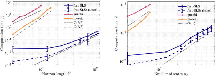
Figure 2: Scalability of different solvers with horizon length for $L=10$ masses (left). Scalability of different solvers with the number of states for horizon $N=20$ (right). The proposed algorithm’s (fast-SLS) computation times, and the Riccati recursions contributions (23) (fast-SLS: riccati) are shown with standard deviations.

In this section, we demonstrate the computational speedup achieved by the proposed algorithm compared to available alternatives. We show how the proposed algorithm scales with increasing horizon and increasing number of states. The nominal trajectory optimization (17) is solved with osqp (Stellato et al., 2020), via its Casadi interface (Andersson et al., 2019), while the Riccati recursions, (23) are implemented using MATLAB.

The proposed algorithm is compared against directly solving the SOCP (7) using general-purpose commercial solvers, Gurobi Optimization (2023) and Mosek ApS (2019), both interfaced using Yalmip (Löfberg, 2004). Computations are carried out on a Macbook Pro equipped with M1 processor with 8 cores and 16 GB of RAM, running macOS Sonoma.

In the following example, we consider a chain of $L$ mass-spring-damper systems as in (Domahidi et al., 2012), corresponding to a linear system with $n_{\mathrm{x}}=2\cdot L$, fixed at one end, with mass $m=1$, spring constant $k=10$, and damper constant $d=2$, and a force actuation on each mass. The system is discretized using a time step $\Delta t=0.5$. We use $Q=P=3{I_{n_{\mathrm{x}}}}$, $R={I_{n_{\mathrm{u}}}}$, $E=0.5I_{n_{\mathrm{x}}}$. The states $x$ and the force input $u$ are constrained at each time step as $\|x\|_{\infty}\leq 4$, and $\|u\|_{\infty}\leq 0.5$. The computation times of the proposed algorithm are calculated based on an average of $30$ randomly sampled feasible initial conditions. We also show the computation times for the Riccati recursions alone (23). We use a convergence tolerance on the primal variables $y$ of $\epsilon_{m}=10^{-8}$, and a minimal tightening of $\epsilon_{\beta}=10^{-10}\bm{1}_{n_{\mathrm{c}}}$.

4.0.1 Convergence

For horizon $N=30$, and $L=6$ masses, we evaluate the number of iterations required to converge for $30$ randomly sampled feasible initial conditions for the proposed solver. In Fig. 3, we see that, in the vast majority of cases, only a few iterations are required to converge to the optimal solution. All the solvers considered converge to the same optimal solution.

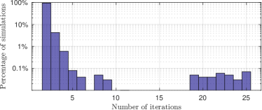
Figure 3: Number of iterations required until convergence for $10^{3}$ randomly sampled initial conditions, for horizon $N=25$, and $L=25$ masses.

4.0.2 Scalability with state dimension

For horizon $N=20$, and an increasing number of masses $L$, we investigate the computation times for different solvers. In Fig. 2 (right), we see that our method scales as $\mathcal{O}(n_{\mathrm{x}}^{3})$, as predicted. The scaling is similar for Mosek and Gurobi. Crucially, the proposed algorithm improves computation times, especially for systems with high state dimension, achieving an improvement in computation speed by factors ranging from $10$ to $10^{3}$ times.

Note 4.1

I am not sure why mosek scalability changes with increasing number of states.

4.0.3 Scalability with horizon length

We investigate the computation times for different solvers, using $L=6$ masses and increasing horizon length $N$. In Fig. 2 (left), we see that our method scales as $\mathcal{O}(N^{2})$. In comparison, Mosek and Gurobi scale respectively approximately as $\mathcal{O}(N^{3})$, and $\mathcal{O}(N^{2})$, indicating the use of a sparse factorization method, as in (Goulart et al., 2008). Crucially, the proposed algorithm improves computation times, especially for long horizons, achieving an improvement in computation speed by factors ranging from $10$ to $10^{3}$ times.

Remark 4.2

As seen in Fig. 2, the computation times are dominated by the Riccati recursions (23). It can be noted that due to overhead in the MATLAB implementation, the computation times are less reliable for small problems. The computation speed of the proposed algorithm could benefit from a more efficient implementation, e.g., relying on the Cholesky decomposition of the cost matrices (21), compare (Frison, 2016).

5 Conclusion

SLS is a flexible technique to jointly optimize the nominal trajectory and controller in robust MPC by using a disturbance feedback parametrization. The resulting SLS-based MPC yields robust constraint satisfaction and provides stability. In this paper, we address the main bottleneck of SLS: the computation times. The proposed algorithm iteratively optimizes the nominal trajectory and then the controller. The nominal trajectory optimization is solved via an efficient QP solver and controller optimizations are solved via Riccati recursions. Each iterate scales with $\mathcal{O}(N^{2}(n_{\mathrm{x}}^{3}+n_{\mathrm{u}}^{3}))$. Leveraging results from Messerer and Diehl (2021), the proposed algorithm locally converges q-linearly to an optimal solution. In a numerical comparison, the proposed algorithm offers speed ups between $10$ and $10^{3}$ compared to general-purpose commercial solvers. We expect that the proposed algorithm can be adapted to address variations of SLS, particularly those involving sparsity or structural constraints.

Appendix A Nonlinear Extension

In the following, we show how the efficient solution to the SOCP (7) can be extended to address nonlinear systems. Based on Leeman et al. (2023a, b), we address robust control of nonlinear systems using the following nonlinear program

$$\min_{\begin{subarray}{c}\mathbf{\Phi}_{\mathbf{x}},\mathbf{\Phi}_{\mathrm{u}},\\ \mathbf{z},\mathbf{v},\bm{\tau}\end{subarray}} J(\mathbf{z},\mathbf{v})+\tilde{H}_{0}(\mathbf{\Phi}),$$ (27a)

s.t. $${z}_{k+1}=\phi(z_{k},v_{k}),~{}{z}_{0}=\bar{x}_{0},~{}k=0,\ldots,N-1,$$ (27b)

$$\bm{\Phi}_{\mathrm{x}}^{k+1,j}=\nabla_{z}\phi\left(z_{k},v_{k}\right)^{\top}\bm{\Phi}_{\mathrm{x}}^{k,j}+\nabla_{v}\phi\left(z_{k},v_{k}\right)^{\top}\bm{\Phi}_{\mathrm{u}}^{k,j},$$ (27c)

$$\bm{\Phi}_{\mathrm{x}}^{j+1,j}=\alpha_{1}^{-1}E_{j}+{\alpha_{2}^{-1}\sqrt{n_{\mathrm{x}}}\mu\tau_{j}^{2}},$$ (27d)

$$j=0,\ldots,N-1,~{}k=j+1,\ldots,N-1,$$

$$\sum_{j=0}^{k-1}\left\|e_{i}^{\top}\mathbf{\Phi}^{k,j}\right\|_{2}-\tau_{k}\leq 0,$$ (27e)

$$i=1,\ldots,n_{\mathrm{x}}+n_{\mathrm{u}},k=0,\ldots,N-1,$$

$$\sum_{j=0}^{k-1}\left\|g_{ki}^{\top}\mathbf{\Phi}^{k,j}\right\|_{2}+g_{ki}^{\top}\left({z}_{k},{v}_{k}\right)+b_{ki}\leq 0,$$ (27f)

$$i=1,\ldots,n_{c},~{}k=0,\ldots,N-1,$$

$$\sum_{j=0}^{N-1}\left\|g_{\mathrm{f}i}^{\top}\bm{\Phi}_{\mathrm{x}}^{N,j}\right\|_{2}+g_{\mathrm{f}i}^{\top}{z}_{N}+b_{\mathrm{f}i}\leq 0,$$ (27g)

$$i=1,\ldots,n_{\mathrm{f}},$$

where $\bm{\tau}\in\mathbb{R}^{N}$ and $e_{i}^{\top}$ is the $i^{\text{th}}$ row of the identity matrix $I_{n_{\mathrm{x}}+n_{\mathrm{u}}}$. The function $\phi:\mathbb{R}^{n_{\mathrm{x}}}\times\mathbb{R}^{n_{\mathrm{u}}}\rightarrow\mathbb{R}^{n_{\mathrm{x}}}$ is assumed to be three times continuously differentiable and is used to define the dynamics (27b), and the disturbance propagation (27c). In (27d) the effect of the additive disturbance $w_{k}$ and the linearization error based on the worst-case curvature $\mu\in\mathbb{R}^{n_{\mathrm{x}}\times n_{\mathrm{x}}}$ of $\phi$ is lumped, see (Leeman et al., 2023a). Here, $\alpha_{1},\alpha_{2}\geq 0$ is used to over-approximate the sum of ellipsoids (Houska, 2011, Thm 2.4) with $\alpha_{1}+\alpha_{2}\leq 1$. The constraints (27e) are used to optimize the dynamic linearization error over-bound $\tau_{k}$, while still jointly optimizing the nonlinear nominal trajectory, and feedback controller, such that robust constraint satisfaction is guaranteed for the nonlinear dynamics using (27f), and (27g).

We write the optimization problem (27) compactly as

$$\min_{y,\mathbf{\Phi},\beta}\quad {J(y)+\tilde{H}_{0}(\mathbf{\Phi})},$$ (28a)

s.t. $$f_{\textrm{nl}}(y)=0,$$ (28b)

$$D_{\textrm{nl}}(y,\mathbf{\Phi})=0,$$ (28c)

$$\tilde{h}(y)+h_{\mathrm{bo}}(\beta)\leq 0,$$ (28d)

$$\tilde{H}(\mathbf{\Phi})-\beta=0,$$ (28e)

where $y:=(\mathbf{z},\mathbf{v},\bm{\tau})$ collects all the nominal trajectory variables, including $\bm{\tau}$. The constraint (28b) corresponds to the nominal trajectory (27b). The disturbance propagation $D_{\textrm{nl}}(y,\mathbf{\Phi})$ in (28c) is linear in $\mathbf{\Phi}$, and (28d), (28e) lump all the inequality constraints (27e), (27f), and (27g).

Algorithm 2 SCP-SLS

$Q$, $R$, $P$, $G_{ki}$, $b_{ki}$, $G_{\mathrm{f}}$, $b_{\mathrm{f}}$

$\bar{M},\bar{\eta},\bar{y}\leftarrow\text{Initialize controller, duals, nominal trajectory}$

while not converged do

     $\nabla f_{\mathrm{nl}}(\bar{y}),\Gamma\bar{\eta}\leftarrow\text{Evaluate gradients}$ $\triangleright$ (33a), (33b)

     $\Delta y,\bar{M}\leftarrow\text{Solve~{}\eqref{eq:reduced_linearized_SLS}}$$\triangleright$ Alg. 1

     $\bar{y}\leftarrow~{}\text{Update nominal}$$\triangleright$ $\bar{y}+\Delta y$

end while

Output: $\mathbf{z}^{\star},~{}\mathbf{v}^{\star},~{}\bm{\tau}^{\star},~{}\bm{\Phi}_{\mathrm{x}}^{\star},~{}\bm{\Phi}_{\mathrm{u}}^{\star}$ satisfy (27)

After substituting (28c) in (28e), similarly as in the linear case Section 3.1, we obtain an equivalent optimization problem

$$\min_{y,M,\beta}\quad {J(y)}+H_{0}(M),$$ (29a)

s.t. $$f_{\mathrm{nl}}(y)=0,$$ (29b)

$$\tilde{h}(y)+h_{\mathrm{bo}}(\beta)\leq 0,$$ (29c)

$$H(M,y)-\beta\leq 0.$$ (29d)

In (29d), we replaced the equality constraint $H(M,y)-\beta\leq 0$ by an inequality, which is convex in $M$. Likewise, the inequality (29c) can be losslessly convexified using auxiliary variables. These modifications do not alter the optimal solution $y$ and $M$ of (29), as the tightenings $\beta$ do not appear in the cost (29a). Applying a standard sequential convex programming (SCP) approach (Tran-Dinh and Diehl, 2010), we first linearize the nonconvex constraints in (29) at $\bar{y}$, $\bar{M}$, yielding

$$\min_{\Delta y,M,\beta}\quad J(\bar{y}+\Delta y)+H_{0}(M)$$ (30a)

s.t. $$f_{\mathrm{nl}}(\bar{y})+\nabla f_{\mathrm{nl}}^{\top}(\bar{y})\Delta y=0,$$ (30b)

$$\tilde{h}(\bar{y}+\Delta y)+h_{\mathrm{bo}}(\beta)\leq 0,$$ (30c)

$$H(M,\bar{y})+\Gamma\Delta y-\beta\leq 0,$$ (30d)

with the gradient

$$\Gamma:=\nabla_{y}H(\bar{M},\bar{y})^{\top}.$$ (31)

Remark A.1

In the SOCP (30), the constraints (30d) only include the linearization with respect to $y$, preserving the advantageous numerical structure of the optimization problem.

In the optimization problem (30), the term $\Gamma\Delta y$ in (30d) prevents the direct use of Algorithm 1 to solve (30). Hence, to be able to use Algorithm 1, and leverage the structure we use a variation of SCP (Bock et al., 2007), where the constraint (30d) is approximated with

$$H(M,\bar{y})-\beta\leq 0.$$ (32)

Due to this inexact Jacobian approximation (Bock et al., 2007), a correction in the cost function (30a) is needed to maintain convergence properties of the SCP scheme. In particular, we iteratively solve a series of optimization problems, equivalent to the SOCP (7):

$$\min_{\Delta y,M,\beta}\quad J(\bar{y}+\Delta y)+H_{0}(M)+\Gamma\bar{\eta}\Delta y,$$ (33a)

s.t. $$f_{\mathrm{nl}}(\bar{y})+\nabla f_{\mathrm{nl}}(\bar{y})^{\top}\Delta y=0,$$ (33b)

$$\tilde{h}(\bar{y}+\Delta y)+h_{\mathrm{bo}}(\beta)\leq 0,$$ (33c)

$$H(M,\bar{y})-\beta\leq 0,$$ (33d)

and iteratively update the optimal nominal trajectory $\bar{y}$ and the optimal dual variable $\bar{\eta}$ associated to (33). Using this approximation, each SOCP iterate (33) has the same structure as (12), and, hence, can be efficiently solved using the proposed algorithm, described in Section 3. Indeed, the inequality in (33d) can be replaced by an equality without changing the optimal solution in $\Delta y$ and $M$. Algorithm 2 summarizes the steps previously outlined.

Under some standard regularity conditions, the SCP based on (33) converges to a KKT point (Messerer et al., 2021) of the original optimization problem (27). In particular, the optimization problems (33) and (30) have the same stationarity conditions.

References

- Alonso and Tseng (2022) Alonso, C.A. and Tseng, S.H. (2022). Effective GPU parallelization of distributed and localized model predictive control. In Proc. 17th International Conference on Control & Automation (ICCA), 199–206. IEEE.
- Anderson et al. (2019) Anderson, J., Doyle, J.C., Low, S.H., and Matni, N. (2019). System level synthesis. Annual Reviews in Control, 47, 364–393.
- Andersson et al. (2019) Andersson, J.A.E., Gillis, J., Horn, G., Rawlings, J.B., and Diehl, M. (2019). CasADi – A software framework for nonlinear optimization and optimal control. Mathematical Programming Computation, 11(1), 1–36. 10.1007/s12532-018-0139-4.
- ApS (2019) ApS, M. (2019). The MOSEK optimization toolbox for MATLAB manual. Version 9.0. URL http://docs.mosek.com/9.0/toolbox/index.html.
- Ben-Tal et al. (2004) Ben-Tal, A., Goryashko, A., Guslitzer, E., and Nemirovski, A. (2004). Adjustable robust solutions of uncertain linear programs. Mathematical programming, 99(2), 351–376.
- Bock et al. (2007) Bock, H.G., Diehl, M., Kostina, E., and Schlöder, J.P. (2007). Constrained optimal feedback control of systems governed by large differential algebraic equations. In Real-Time PDE-constrained optimization, 3–24. SIAM.
- Chen et al. (2022) Chen, S., Preciado, V.M., Morari, M., and Matni, N. (2022). Robust model predictive control with polytopic model uncertainty through system level synthesis. arXiv preprint arXiv:2203.11375.
- Domahidi et al. (2012) Domahidi, A., Zgraggen, A.U., Zeilinger, M.N., Morari, M., and Jones, C.N. (2012). Efficient interior point methods for multistage problems arising in receding horizon control. In Proc. 51st IEEE Conference on Decision and Control (CDC), 668–674. IEEE.
- Frison (2016) Frison, G. (2016). Algorithms and methods for high-performance model predictive control. Ph.D. thesis, Technical University of Denmark.
- Frison and Diehl (2020) Frison, G. and Diehl, M. (2020). HPIPM: a high-performance quadratic programming framework for model predictive control. IFAC-PapersOnLine, 53(2), 6563–6569.
- Giftthaler et al. (2018) Giftthaler, M., Neunert, M., Stäuble, M., Buchli, J., and Diehl, M. (2018). A family of iterative gauss-newton shooting methods for nonlinear optimal control. In Proc. International Conference on Intelligent Robots and Systems (IROS), 1–9. IEEE.
- Goulart et al. (2006) Goulart, P.J., Kerrigan, E.C., and Maciejowski, J.M. (2006). Optimization over state feedback policies for robust control with constraints. Automatica, 42(4), 523–533.
- Goulart et al. (2008) Goulart, P.J., Kerrigan, E.C., and Ralph, D. (2008). Efficient robust optimization for robust control with constraints. Mathematical Programming, 114(1), 115–147.
- Gurobi Optimization (2023) Gurobi Optimization (2023). Gurobi Optimizer Reference Manual. URL https://www.gurobi.com.
- Houska (2011) Houska, B. (2011). Robust optimization of dynamic systems. Ph.D. thesis, Katholieke Universiteit Leuven.
- Howell et al. (2019) Howell, T.A., Jackson, B.E., and Manchester, Z. (2019). Altro: A fast solver for constrained trajectory optimization. In Proc. International Conference on Intelligent Robots and Systems (IROS), 7674–7679. IEEE.
- Kim et al. (2022) Kim, T., Elango, P., and Acikmese, B. (2022). Joint synthesis of trajectory and controlled invariant funnel for discrete-time systems with locally lipschitz nonlinearities. arXiv preprint arXiv:2209.03535.
- Köhler et al. (2020) Köhler, J., Soloperto, R., Müller, M.A., and Allgöwer, F. (2020). A computationally efficient robust model predictive control framework for uncertain nonlinear systems. IEEE Trans. Automat. Contr., 66(2), 794–801.
- Kouzoupis et al. (2018) Kouzoupis, D., Frison, G., Zanelli, A., and Diehl, M. (2018). Recent advances in quadratic programming algorithms for nonlinear model predictive control. Vietnam Journal of Mathematics, 46(4), 863–882.
- Leeman et al. (2023a) Leeman, A.P., Köhler, J., Zanelli, A., Bennani, S., and Zeilinger, M.N. (2023a). Robust nonlinear optimal control via system level synthesis. arXiv preprint arXiv:2301.04943.
- Leeman et al. (2023b) Leeman, A.P., Sieber, J., Bennani, S., and Zeilinger, M.N. (2023b). Robust optimal control for nonlinear systems with parametric uncertainties via system level synthesis. In Proc. 62nd IEEE Conference on Decision and Control (CDC), 4784–4791. IEEE.
- Li and Todorov (2004) Li, W. and Todorov, E. (2004). Iterative linear quadratic regulator design for nonlinear biological movement systems. In Proc. First International Conference on Informatics in Control, Automation and Robotics, volume 2, 222–229. SciTePress.
- Li et al. (2023) Li, Z., Hu, C., Zhao, W., and Liu, C. (2023). Learning predictive safety filter via decomposition of robust invariant set. arXiv preprint arXiv:2311.06769.
- Löfberg (2004) Löfberg, J. (2004). YALMIP : A toolbox for modeling and optimization in matlab. In Proc. of the CACSD Conference. Taipei, Taiwan.
- Majumdar and Tedrake (2017) Majumdar, A. and Tedrake, R. (2017). Funnel libraries for real-time robust feedback motion planning. The Int. Journal of Robotics Research, 36(8), 947–982.
- Manchester and Kuindersma (2017) Manchester, Z. and Kuindersma, S. (2017). DIRTREL: Robust trajectory optimization with ellipsoidal disturbances and LQR feedback. In Proc. Robotics: Science and Systems (RSS), Cambridge. 10.15607/RSS.2017.XIII.057.
- Mayne et al. (2005) Mayne, D.Q., Seron, M.M., and Raković, S. (2005). Robust model predictive control of constrained linear systems with bounded disturbances. Automatica, 41(2), 219–224.
- Messerer et al. (2021) Messerer, F., Baumgärtner, K., and Diehl, M. (2021). Survey of sequential convex programming and generalized gauss-newton methods. ESAIM: Proceedings and Surveys, 71, 64–88.
- Messerer and Diehl (2021) Messerer, F. and Diehl, M. (2021). An efficient algorithm for tube-based robust nonlinear optimal control with optimal linear feedback. In Proc. 60th Conference on Decision and Control (CDC), 6714–6721. IEEE.
- Neunert et al. (2016) Neunert, M., De Crousaz, C., Furrer, F., Kamel, M., Farshidian, F., Siegwart, R., and Buchli, J. (2016). Fast nonlinear model predictive control for unified trajectory optimization and tracking. In Proc. International conference on robotics and automation (ICRA), 1398–1404. IEEE.
- Rao et al. (1998) Rao, C.V., Wright, S.J., and Rawlings, J.B. (1998). Application of interior-point methods to model predictive control. Journal of optimization theory and applications, 99, 723–757.
- Rawlings et al. (2017) Rawlings, J.B., Mayne, D.Q., and Diehl, M. (2017). Model predictive control: theory, computation, and design, volume 2. Nob Hill Publishing Madison, WI.
- Schulman et al. (2014) Schulman, J., Duan, Y., Ho, J., Lee, A., Awwal, I., Bradlow, H., Pan, J., Patil, S., Goldberg, K., and Abbeel, P. (2014). Motion planning with sequential convex optimization and convex collision checking. The International Journal of Robotics Research, 33(9), 1251–1270.
- Scokaert and Mayne (1998) Scokaert, P. and Mayne, D. (1998). Min-max feedback model predictive control for constrained linear systems. IEEE Trans. Automat. Contr., 43(8), 1136–1142. 10.1109/9.704989.
- Sieber et al. (2021) Sieber, J., Bennani, S., and Zeilinger, M.N. (2021). A system level approach to tube-based model predictive control. IEEE Control Systems Letters, 6, 776–781.
- Sieber et al. (2023) Sieber, J., Zanelli, A., Leeman, A., Bennani, S., and Zeilinger, M.N. (2023). Asynchronous computation of tube-based model predictive control. In IFAC World Congress.
- Steinbach (1995) Steinbach, M. (1995). Fast recursive SQP methods for large-scale optimal control problems. Ph.D. thesis, Universität Heidelberg.
- Stellato et al. (2020) Stellato, B., Banjac, G., Goulart, P., Bemporad, A., and Boyd, S. (2020). OSQP: an operator splitting solver for quadratic programs. Mathematical Programming Computation, 12(4), 637–672.
- Tran-Dinh and Diehl (2010) Tran-Dinh, Q. and Diehl, M. (2010). Local convergence of sequential convex programming for nonconvex optimization. In Recent Advances in Optimization and its Applications in Engineering: The 14th Belgian-French-German Conference on Optimization, 93–102. Springer.
- Tseng et al. (2020) Tseng, S.H., Alonso, C.A., and Han, S. (2020). System level synthesis via dynamic programming. In Proc. 59th Conference on Decision and Control (CDC), 1718–1725. IEEE.
- Villanueva et al. (2017) Villanueva, M.E., Quirynen, R., Diehl, M., Chachuat, B., and Houska, B. (2017). Robust MPC via min–max differential inequalities. Automatica, 77, 311–321.
- Wright et al. (1999) Wright, S., Nocedal, J., et al. (1999). Numerical optimization. Springer Science.
- Zanelli et al. (2021) Zanelli, A., Frey, J., Messerer, F., and Diehl, M. (2021). Zero-order robust nonlinear model predictive control with ellipsoidal uncertainty sets. IFAC-PapersOnLine, 54(6), 50–57.