A Systematic Approach to Robustness Modelling for Deep Convolutional Neural Networks

Abstract

Convolutional neural networks have shown to be widely applicable to a large number of fields when large amounts of labelled data are available. The recent trend has been to use models with increasingly larger sets of tunable parameters to increase model accuracy, reduce model loss, or create more adversarially robust models—goals that are often at odds with one another. In particular, recent theoretical work raises questions about the ability for even larger models to generalize to data outside of the controlled train and test sets. As such, we examine the role of the number of hidden layers in the ResNet model, demonstrated on the MNIST, CIFAR10, CIFAR100 datasets. We test a variety of parameters including the size of the model, the floating point precision, and the noise level of both the training data and the model output. To encapsulate the model’s predictive power and computational cost, we provide a method that uses induced failures to model the probability of failure as a function of time and relate that to a novel metric that allows us to quickly determine whether or not the cost of training a model outweighs the cost of attacking it. Using this approach, we are able to approximate the expected failure rate using a small number of specially crafted samples rather than increasingly larger benchmark datasets. We demonstrate the efficacy of this technique on both the MNIST and CIFAR10 datasets using 8-, 16-, 32-, and 64-bit floating-point numbers, various data pre-processing techniques, and several attacks on five configurations of the ResNet model. Then, using empirical measurements, we examine the various trade-offs between cost, robustness, latency, and reliability to find that larger models do not significantly aid in adversarial robustness despite costing significantly more to train.

1 Introduction

Machine Learning (ML) has become a widely popular tool for solving complex problems across many disciplines, like medical imaging [Erickson et al., 2017], computer security [Arp et al., 2022], law enforcement [Travaini et al., 2022], aviation [Maheshwari et al., 2018], and parcel scanning Mery et al. [2016]. Despite this, adversarial attacks aim to exploit vulnerabilities in machine learning models by introducing subtle modifications to data submitted to various stages of the ML pipeline, leading to misclassification or otherwise erroneous outputs [Chakraborty et al., 2018]. Ensuring the robustness of ML models against adversaries has become a critical concern [Brown et al., 2017, Carlini and Wagner, 2017, Croce and Hein, 2020, Chen et al., 2020, Nicolae et al., 2018, Meyers et al., 2023]. However, understanding the relationship between computational cost and the performance against adversarial noise remains an ongoing challenge. In this work, we investigated the robustness of various deep neural networks and data pre-processing techniques against adversarial attacks and explore the relationship between computational cost and prediction accuracy in both benign and adversarial contexts. By using samples crafted specifically to be challenging and applying accelerated failure rate models (see Sec. 3) we provide a method for estimating the expected failure time across the entire feasible adversarial space. Using this model, we demonstrate that larger models, while offering marginal gains over smaller models, do so at the expense of training times that far outpace the expected adversarial training time.

1.1 Motivations

It is routine to think in this adversarial context when considering safety- or security- critical applications Erickson et al. [2017], Arp et al. [2022], Travaini et al. [2022], Maheshwari et al. [2018], Mery et al. [2016] where we assume the attacker is operating in their best-case scenario Leurent and Peyrin [2020], Kamal [2017], Madry et al. [2017], Kotyan and Vargas [2022], Moosavi-Dezfooli et al. [2016], Croce and Hein [2020]. A recent study Kamal [2017] distilled the process of password-cracking into an cloud-native service that can break common password schemes in a number of days. Another paper Leurent and Peyrin [2020], defines ‘broken’ in the context of time to highlight the ease with which one can subvert a particular hashing algorithm. However, someone attacking a machine learning model might have a variety of competing goals that optimize the perturbation distance, number of queries, or other metrics Madry et al. [2017], Chen et al. [2020], Kotyan and Vargas [2022], Goodfellow et al. [2014], Moosavi-Dezfooli et al. [2016]. Much work has gone into mitigating the detrimental effects of these attacks, for example by adding noise in the training process Zantedeschi et al. [2017], Lecuyer et al. [2019], rejecting low-confidence results without penalty Chen et al. [2021], or reducing the bit-depth of the data and model weights Xu et al. [2017]. However, these analyses focus on ad-hoc posterior evaluations on benchmark datasets (namely CIFAR-10 and MNIST) to determine whether or not a given technique is more- or less-effective than another. That is, the relationship between marginal benefit and marginal cost is unclear. Furthermore, the community has relied on larger models Desislavov et al. [2021] and larger datasets Desislavov et al. [2021], Bailly et al. [2022] to yield increasingly marginal gains Sun et al. [2017]. In order to reach safety-critical standards routine in other industries International Standards Organization [2018], International Electrotechnical Commission [2010, 2006], we must move beyond the limited test/train split paradigm that would require many, many billions of samples for every change of a neural network Meyers et al. [2023]. So, first, discuss failure rates and cost in the context of deep neural networks (see Section 2.2). Second, we demonstrate how to model the failure rate as a function of time (see Section 3) using accelerated methods. Third, we extend this time-dependent concept of ‘broken’ algorithms from cryptography into machine learning (see Section 4). Using this, we can quickly and precisely investigate the effects of various attacks (see Section 5.4), defences (see Section 5.3), and model architectures (see Section 5.2).

1.2 Contributions

We summarize our contributions below:

• We propose to use accelerated failure time methods for analyzing ML models under adversarial perturbations and provide substantial empirical evidence that this method is both effective and dataset-agnostic, allowing us to predict the expected failure rate more precisely and accurately than with either adversarial or benign accuracy alone.

• We use accelerated failure time models to measure model robustness across a wide variety of signal pre-processing techniques to explore the relationships between latency, accuracy, and model depth.

• We introduce a metric for evaluating whether or not a model is robust to adversarial attacks in a time- and compute-constrained context.

• We use this metric to show that, at best, increasing the number of hidden layers in a neural network increases training time while having little-to-no benefit in the presence of an adversary.

2 Background

Much work has already gone into explaining the dangers of adversarial attacks on ML pipelines [Carlini and Wagner, 2017, Croce and Hein, 2020, Kotyan and Vargas, 2022, Goodfellow et al., 2014, Biggio et al., 2013a] though that work is limited to ad-hoc and posterior evaluations against limited sets of attack and defence parameters, leading to results that are, at best, overconfident [Meyers et al., 2023, Ma et al., 2020]. Here, we are addressing evasion [Carlini and Wagner, 2017] attacks that attempt to induce a misclassification at run-time though our analysis extends to other types of attacks like database poisoning [Biggio et al., 2013b, Saha et al., 2020], model inversion [Choquette-Choo et al., 2021, Li and Zhang, 2021], or data stealing [Orekondy et al., 2019]. This work formalizes methods for quantifying the adversarial failure rate of a model and comparing the efficacy of model changes in the context of fixed compute budget.

2.1 Adversarial Attacks

In the context of ML, an adversarial attack refers to deliberate and malicious attempts to manipulate the behavior of ML models. These attacks are designed to change the model’s behavior by introducing carefully crafted input data that can cause the model to make incorrect predictions or otherwise produce undesired outputs. The goal of an attacker is often to exploit vulnerabilities in the model’s decision-making process or to probe its weaknesses. These attacks can occur during various stages of the ML pipeline, including during training [Biggio et al., 2013b], inference[Biggio et al., 2013a], or deployment [Santos et al., 2021]. For all sections below, we collect metrics on the benign (unperturbed) data and adversarial (perturbed) data. The abbreviations ben. and adv. are used throughout, respectively.

2.1.1 Perturbation Distance

The strength of an attack is generally though of in terms of perturbation ‘distance’ [Croce and Hein, 2020, Chakraborty et al., 2018, Kotyan and Vargas, 2022]. The perturbation distance, denoted by $\varepsilon$, quantifies the magnitude of the perturbation applied to a sample, $x$, when generating a new adversarial sample, $x^{\prime}$. The perturbation distance is usually defined using some norm (or pseudo-norm). The definition is,

$$\varepsilon:=\|x^{\prime}-x\|\leq\varepsilon_{max},$$

where $\|\cdot\|$ denotes a norm or pseudo-norm (e.g., the Euclidean $\ell_{2}$ norm or the $\ell_{0}$ pseudo-norm). We denote by $\varepsilon_{max}$ the maximum allowed deviation or distortion from the original input while still being within the feasible sample space. For example, this might be one bit, one pixel, or one byte, depending on the test conditions. For more information on different optimization criteria, see Section 5.4.

2.1.2 Accuracy and Failure Rate

The accuracy refers to the percentage or proportion of examples that cause the targeted ML model to misclassify or produce incorrect outputs and is a measure of the vulnerability or susceptibility of the model to noise-induced failures. A lower accuracy indicates a higher rate of misclassifications or incorrect predictions. The accuracy, $\lambda$, is defined as:

$$\lambda:=1-\frac{\textrm{False~{}Classifications}}{N},$$ (1)

where $N$ is the number of samples. However, accuracy is known to vary with things like model complexity Simonyan and Zisserman [2014], He et al. [2016], data resolution Xu et al. [2017], the number of samples Vapnik et al. [1994] , the number of classes  Dohmatob [2019], or the amount of noise in the data Zantedeschi et al. [2017], Lecuyer et al. [2019], Dohmatob [2019]. Likewise, there are many hyperparameters that can influence an attack’s run time and accuracy. Instead, we can think in terms of failure rate:

$$\mathrm{Failure~{}Rate}:=\frac{\mathrm{False~{}Classifications}}{\Delta t},$$ (2)

where $\Delta t$ is a time interval. This failure rate varies as a function of time, and we would like to model this behaviour. So, let $h$ be a function with model/attack parameters, $\theta$, such that $h_{\theta}$ describes the rate of failure at time $t$. We can express the failure rate in terms of a hazard function, which can be expressed in terms of a point in time, $t$. It is defined as:

$$h_{\theta}(t):=\lim_{\Delta t\rightarrow 0}\frac{P(t\leq T<t+\Delta t\,|\,T\geq t)}{\Delta t},$$ (3)

where $T$ is time until a false classification occurs, also referred to as survival time Kleinbaum and Klein [1996]. To describe the computational efficacy of different model and attack configurations in general, we modelled the probability of not observing a failure before a given time, $t$, giving the cumulative survival function,

$$S_{\theta}(t):=\exp\left\{-\int_{0}^{t}h_{\theta}(\tau)d\tau)\right\}.$$ (4)

The probability density of observing a failure at time, $t$, is Kleinbaum and Klein [1996],

$$f(t;\theta):=h_{\theta}(t)S_{\theta}(t).$$

If we assume the probability of failure and time-to-failure is uniform across the samples for a particular set of covariates, we can estimate the probability of failure on the unperturbed test set,

$$f_{ben.}(t;\theta)\approx\frac{1-\lambda_{ben.}}{t_{predict}}\cdot t,$$ (5)

where $t_{predict}$ indicates the inference time per sample. As we can plainly see, at $t=t_{predict}$, this reduces to one minus the test-set benign accuracy. However, this is, at best, an optimistic lower bound to the the real-world failure rate Meyers et al. [2023], Croce and Hein [2020]. To get a realistic picture of the worst-case scenario, we can look at $f$ in the presence of adversarial noise,

$$f_{adv.}(t;\theta)\approx\frac{1-\lambda_{adv.}}{t_{attack}}\cdot t,$$ (6)

where $t_{attack}$ refers to the attack generation time per sample. Hence, at $t=t_{attack}$ this reduces to one minus the adversarial accuracy.

2.2 Cost

For our purposes, we assumed the cost, $C_{train}$, is proportional to the total training, $T_{train}$, the number of samples, $N$, and the training time per sample, $t_{\mathrm{train}}$, such that the cost of training on hardware with a fixed time-cost, $C_{h}$, is

$$C_{train}:=C_{h}\cdot T_{\mathrm{train}}=C_{h}\cdot t_{train}\cdot N,$$

where $C_{h}$ is the cost per time unit of a particular piece of hardware. This assumption means that cost will scale linearly with per-sample training time or sample size. Analogously, we can discuss this in adversarial terms where $N$ is the number of samples. If we assume the same hardware cost as the model-builder then,

$$C_{attack}:=C_{h}\cdot T_{\mathrm{attack}}=C_{h}\cdot t_{attack}\cdot N.$$

If we assume that the training time and attack time are uniform across the samples and restricted to the same hardware, then we can say that

$$C_{train}\propto t_{train}\text{~{}~{}~{}and~{}~{}~{}}C_{attack}\propto t_{attack}.$$ (7)

Furthermore, a fast attack will be lower-bounded by $t_{predict}$, which is generally much smaller than the training time, $t_{train}$. Of course the long-term costs of deploying a model will be related to the inference cost, but a model is clearly broken if the cost of improving a model ($\propto t_{train}$) is much, much larger than the cost of finding a counterexample ($\propto t_{attack}$) within some imperceptible noise distance of untainted samples. However, this merely encapsulates the cost of a particular model architecture or signal pre-processing choice and doesn’t consider the likelihood of noise induced failure. Our cost normalized metric is introduced below in Eq. 8 in Section 4. Before we can compare this cost to the failure rate, we must estimate the attack time per sample, or expected survival time, $\mathbb{E}[T]$. For that, we use an accelerated failure rate model.

3 Accelerated Failure Models for ML

Failure rate analysis has been widely explored in other fields [Bradburn et al., 2003] from medicine to industrial quality control [Erickson et al., 2017, Koay et al., 2023, Maheshwari et al., 2018, Mery et al., 2016, Arp et al., 2022, Travaini et al., 2022], but there’s very little published research in the context of ML. However, as noted by many researchers [Madry et al., 2017, Carlini and Wagner, 2017, Croce and Hein, 2020, Meyers et al., 2023], these models are fragile to attackers that intend to subvert the model, steal the database, or evade detection. Accelerated Failure Rate (AFR) models have been widely used to investigate the causes and likelihood of failures across fields where safety is a primary concern (e.g., in medicine, aviation, or automobiles). When, for example, a car manufacturer wants to test a motor for next-year’s production model, they cannot simply sample a collection of motors from their upstream suppliers since the motor is intended to last a decade or more. Instead, they induce failures by introducing extreme circumstances [Liu et al., 2013, Lawless et al., 1995] into the verification procedures. For example, this might include running the motor in extremely cold or hot environments, cycling between temperatures rapidly, or using extreme vibration to accelerate the effect of normal wear-and-tear [Meeker et al., 1998]. By measuring the effect of each of these test scenarios on the tested component and keeping track of the real-world circumstances and usage of their products, they can estimate the long-term behavior of a component without relying on long-term testing that would drastically slow development. That is, they can successfully estimate the expected survival time of a component using accelerated methods.

Under the assumption of accelerated failure time Kleinbaum and Klein [1996], we can express the survival time as,

$$S_{\theta}(t)=S_{0}(\phi(\theta,x)t),$$

where $\phi$ is an acceleration factor that depends on the covariates, typically $\phi(\theta,x)=\exp{(\theta_{1}x_{1}+\theta_{2}x_{2}+\cdots+\theta_{p}x_{p})}$ and $S_{0}$ is the baseline survivor function. For example, the covariates might be things like perturbation distance, model depth, or number of training epochs. We can use the survival function to compute the expected survival time,

$$\mathbb{E}_{S_{\theta}}[T]=\int_{0}^{\infty}t\cdot S_{\theta}(t)\,dt.$$

While non-parametric AFR models like Cox’s proportional hazard model do exist, they don’t allow us to estimate the underlying distribution Kleinbaum and Klein [1996] — merely the proportional effects of the covariates [Bradburn et al., 2003]. Furthermore, parametric distributions are known to be robust to omitted covariates [Lambert et al., 2004].

3.1 Weibull AFR

The first AFR model we tested was using the Weibull distribution, which has the form

$$S_{\theta}(t;x,y)=\exp{\left(-\left(\frac{t}{\lambda(\beta,x)}\right)^{\rho(\alpha,y)}\right)},$$

where $\theta=(\alpha,\beta)$, the $x=(x_{1},\ldots,x_{p})$ is the set of covariates and $y=(y_{1},\ldots,y_{n})$ is the count of failure events, and where $\lambda(\beta,x)=\exp(\beta_{0}+\beta_{1}x_{1}+\cdots+\beta_{n}x_{p})$ is a scale parameter and $\rho(\alpha,y)=\exp(\alpha_{0}+\alpha_{1}y_{1}+\cdots+\alpha_{p}y_{p})$ is a shape parameter that determines the direction of acceleration over time.

3.2 Log-Normal AFR

The Log-Normal AFR model introduces the parameters $\mu(\alpha,x)=\alpha_{0}+\alpha_{1}x_{1}+\cdots+\alpha_{n}x_{p}$ and $\sigma(\beta,y)=\exp(\beta_{0}+\beta_{1}y_{1}+\cdots+\beta_{n}y_{p})$ with the survival function given by,

$$S_{\theta}(t;x,y)=1-\log\left(1-\Phi\left(\frac{\log(t)-\mu(\alpha,x)}{\sigma(\beta,y)}\right)\right),$$

where $\theta=(\alpha,\beta)$.

3.3 Log-Logistic AFR

Another form of the AFR model, the Log-Logistic AFR, introduces the scale and shape parameters $a(\alpha,x)=\exp(\alpha_{0}+\alpha_{1}x_{1}+\cdots+\alpha_{n}x_{p})$ and $b(\beta,y)=\exp(\beta_{0}+\beta_{1}y_{1}+\cdots+\beta_{n}y_{p})$, respectively, with survival function,

$$S_{\theta}(t;x,y)=1-\log\left(1+\left(\frac{t-a(\alpha,x)}{b(\beta,y)}\right)\right),$$

where $\theta=(\alpha,\beta)$.

3.4 AFR Model Comparison Scores

To compare the efficacy of different parametric aft models, we use the Akaike information criterion (AIC), log-likelihood, concordance score, and the Bayesian information model  [Stoica and Selen, 2004, Taddy, 2019]. In particular we note that a concordance index $>.5$ indicates that the failure rate is a function of time, undermining the efficacy of the time-independent train/test split methodology that is standard in the literature Longato et al. [2020].

4 Failure Rates and Cost Normalization

So, finally, we can introduce the idea of a failure rate normalized cost. If we assume that the cost scales linearly with $t_{train}$ (Eq. 7), then we can normalize it by the expected survival time to get a rough estimate of the relative costs for the model builder ($C_{train}\propto t_{train}$) or the attacker ($C_{adv.}=\mathbb{E}_{S_{\theta}}[T]\approx t_{attack}$). Recalling the definition of $\varepsilon$ from Section 2.1.1, we can separately consider the cases $\varepsilon=0$ and $\varepsilon>0$. Then, we can express this relative cost of failure in both benign and adversarial terms as,

$$\bar{C}_{ben.}=\frac{t_{train}}{\mathbb{E}_{S_{\theta}}[T\,|\,\varepsilon=0]}\text{~{}~{}~{}and~{}~{}~{}}\bar{C}_{adv.}=\frac{t_{train}}{\mathbb{E}_{S_{\theta}}[T\,|\,0<\varepsilon\leq\varepsilon_{max}]}.$$ (8)

If $\bar{C}\gg 1$ (in either case) then it’s clear that our approach is invalid (e.g., that our model is broken). Also, if you treat $\varepsilon$ as a covariate in ${S_{\theta}}(t)$, then these costs can be computed from the same model. This approach has two advantages over the traditional train-test split method. Firstly, we can quantify the effects of covariates like model depth or noise distance to compare the effect of model changes. Secondly, the train-test split methodology relies on an ever-larger number of samples to increase precision, whereas the accelerated failure method is able to precisely and accurately compare models using only a small number of samples Schmoor et al. [2000], Lachin [1981] relative to the many billions required of the train/test split methodology and safety-critical standards International Standards Organization [2018], International Electrotechnical Commission [2010, 2006], Meyers et al. [2023]. In short, by generating worst-case examples (e.g., adversarial ones), we can test and compare arbitrarily complex models before they leave the lab, drive a car, predict the presence of cancer, or pilot a drone.

5 Methodology

Below we outline the experiments performed and the hyper-parameter configurations across the various model architectures, model defences, and attacks. All experiments were conducted on Ubuntu 18.04 in a virtual machine running in a shared-host environment with one NVIDIA V100 GPU using Python 3.8.8. All configurations were tested in a grid search using hydra [Yadan, 2019] to manage the parameters, dvc [dvc.org, 2023] to ensure reproducibility, and optuna [Akiba et al., 2019] to manage the scheduling. For each attack and model configuration, we collected the metrics outlined in Eqs. 1–8 as well as inference time, training time, and attack generation time. We conducted a grid search of datasets, models, defences, and attacks across 10 shufflings of the data. To generate the figures, we selected the Pareto set Jahan et al. [2016] using the paretoset [tommyod, 2020] package, selecting the subset of experiments that either maximized the accuracy or minimzed the adversarial accuracy for each model, defence, and attack for each specified value. For visualization, we approximated $f_{ben.}$ and $f_{adv.}$ for each attack and defence combination using Eqs. 5 and approximated $\bar{C}$ in the adversarial and benign scenarios as per Eq. 8

5.1 Dataset

Experiments were performed on both the CIFAR100, CIFAR10 [Krizhevsky et al., 2009], and MNIST [Deng, 2012] datasets. We measured the adversarial/benign accuracies, the attack generation time, and the prediction time. To calculate the adversarial failure rate and the cost we used Eqs. 2 & 8. For accuracy, see: Eq. 1. We trained on 80% of the samples for all datasets. Of the remaining 20%, one-hundred class-balanced samples were selected from this test set to evaluate each attack. In addition, the data were shuffled to provide us with 10 samples for each configuration. Then, the data were centered and scaled by the using the parameters defined by the training set to avoid data leakage.

5.2 Tested Models

The Residual Neural Network (ResNet) [He et al., 2016] is a popular classification model because of its ability to train neural networks with many layers efficiently through residual connections. Deep networks, e.g., VGG [Simonyan and Zisserman, 2014], ResNet [He et al., 2016], rely on the depth of the network, which, despite leading to more accurate or robust results [Rolnick and Tegmark, 2017, Carlini and Wagner, 2017], tends to lead to the ‘vanishing gradient problem’ [Hochreiter, 1998], making learning difficult and slow. However, the residual connections allow models to have hundreds of layers rather than tens of layers [He et al., 2016, Simonyan and Zisserman, 2014]. Despite the prevalence of the reference architecture, several modifications have been proposed that trade off, for instance, robustness and computational cost by varying the number of convolutional layers in the model. We tested the Resnet-18, -34, -51, -101, and -152 reference architectures, that get their names from their respective number of layers. We used the the pytorch framework and the Stochastic Gradient Descent minimizer with a momentum parameter of 0.9 and learning rates $\in\{10,1,0.1,0.01,0.001,0.0001,.00001,0.000001\}$ for epochs $\in\{10,20,30,50,100\}$. The learning rate that maximized the benign accuracy for a given layer/defence configuration was used in further analyses (i.e., the learning rate was tuned). In a separate experiment, we also evaluated the different Resnet models across epochs $\in\{10,20,30,50,100\}$.

5.3 Tested Defences

In order to simulate various conditions affecting the model’s efficacy, we have also tested several defences that modify the model’s inputs or predictions in an attempt to reduce its susceptibility to adversarial perturbations. Just like with the attacks, we used the Adversarial Robustness Toolbox [Nicolae et al., 2018] for their convenient implementations. These defences are listed below.

• Gauss-in ($\ell_{2}$): the ‘Gaussian Augmentation’ defence adds Gaussian noise to some proportion of the training samples. In our case, we set this proportion to 50%, allowing us to simulate the effect of noise on the resulting model [Zantedeschi et al., 2017]. We tested noise levels in $\{.001,.01,.1,.3,.5,1\}$.

• Conf : ($\ell_{\infty}$) the ‘High Confidence Thresholding’ defence only returns a classification when the specified confidence threshold is reached, resulting in a failed query if a classification is less certain. This allows us to simulate the effects of rejecting ‘adversarial’ or otherwise ‘confusing’ queries [Chen et al., 2021] that fall outside of given confidence range by ignoring ambiguous results without penalty. We tested confidence levels in $\{.1,.5,.9,.99,.999\}$.

• Gauss-out ($\ell_{2}$): the ‘Gaussian Noise‘ defence, rather than adding noise to the input data, it adds noise to the model outputs [Lecuyer et al., 2019], allowing us to simulate small changes in model weights without going through costly training iterations. We tested levels in $\{.001,.01,.1,.3,.5,1\}$.

• FSQ : the ‘Feature Squeezing‘ defence changes the bit-depth of the input data in order to minimize the noise induced by floating point operations. We include it here to simulate the effects of various GPU or CPU architectures, which may also vary in bit-depth [Xu et al., 2017]. We tested bit-depths in $\{2,4,8,16,32,64\}$.

5.4 Tested Attacks

In order to simulate various attacks that vary in information and run-time requirements across a variety of distance metrics, we have evaluated several attacks using the Adversarial Robustness Toolbox [Nicolae et al., 2018]. Other researchers [Carlini and Wagner, 2017] have noted the importance of testing against multiple types of attacks. For our purposes, attack strength refers to the degree to which an input is modified by an attacker, as described in Sec. 2.1.1. Below, we briefly describe the attacks that we tested against. One or more norms or pseudo-norms were used to optimise each attack, denoted in the parentheses next to the attack name.

• FGM ($\ell_{1},\ell_{2},\ell_{\infty}$): the ‘Fast Gradient Method’ quickly generates noisy sample with no feasibility conditions beyond a specified step size and number of iterations [Goodfellow et al., 2014] by using the model gradient and taking a step of length $\varepsilon$ in the direction that maximizes the loss with $\varepsilon\in\{.001,.01,.03,.1,.2,.3,.5,.8,1\}$.

• PGD ($\ell_{1},\ell_{2},\ell_{\infty}$): the ‘Projected Gradient Method’ extends the FGM attack to include a projection on the $\varepsilon$-sphere, ensuring that generated samples do not fall outside of the feasible space [Madry et al., 2017]. This algorithm is iterative and we restricted it to ten such iterations. In short, this imposes feasibility conditions on the FGM attack with $\varepsilon\in\{001,.01,.03,.1,.2,.3,.5,.8,1\}$.

• Pixel ($\ell_{0}$): the ‘Pixel’ attack [Kotyan and Vargas, 2022] is a multi-objective attack that seeks to minimize the number of perturbed pixels while maximizing the false confidence using a classic multi-objective search function called NSGA2 [Deb et al., 2002]. This algorithm is iterative and we restricted it to ten such iterations. The control parameter for this was the number of perturbed pixels $\varepsilon\in\{4,16,64,256\}$.

• Thresh ($\ell_{\infty})$: the ‘Threshold’ attack also uses the same multi-objective search algorithm as Pixel to optimize the attack, but tries to maximize false confidence while minimizing the $\ell_{2}$ perturbation distance. This algorithm is iterative and we restricted it to ten such iterations.

• Deep ($\ell_{2}$): the Deepfool Attack [Moosavi-Dezfooli et al., 2016] finds the minimal separating hyperplane between two classes and then adds a specified amount of perturbation to ensure it crosses the boundary by using an approximation of the model gradient including the top $n$ outputs where $n\in\{1,3,5,10\}$, speeding up computation by ignoring unlikely classes [Moosavi-Dezfooli et al., 2016]. This algorithm is iterative and we restricted it to ten such iterations.

• HSJ ($\ell_{2}$, queries): the ‘HopSkipJump’ attack, in contrast to the attacks above, does not need access to model gradients nor soft class labels, instead relying on an offline approximation of the gradient using the model’s decision boundaries. In this case, the strength is denoted by the number of queries necessary to find an adversarial counterexample [Chen et al., 2020]. This algorithm is iterative and we restricted it to ten such iterations.

5.5 Identification of ResNet Model-, Defence- and Attack-Specific Covariates

For each attack type, we identified the attack-specific distance metric (or pseudo-metric) outlined in Sec. 5.4. To compare the effect of this measure against other attacks, the valued were min-max scaled so that all values fell on the interval $[0,1]$. For defences, we did the same scaling. However, while a larger number always means more (marginal) noise in the case of attacks, a larger value for the FSQ defence indicates a larger bit-depth and more floating point error. For Gauss-in and Gauss-out, a larger number does indicate more noise, but a larger number for Conf indicates a larger rejection threshold for less-than-certain classifications, resulting in less low-confidence noise. For the models we tracked the number of epochs and the number of layers as well as the training and inference times.

5.6 AFR Models

We tested the Weibull, Log-Normal, and Log-Logistic AFR models using the lifelines [Davidson-Pilon, 2019] package in Python, relying on the metrics outlined in Section 3.4 for comparison since they are widely used in the AFR literature [Bradburn et al., 2003].

6 Results and Discussion

Through tens of thousands experiments across many signal-processing techniques (e.g., defences), random states, learning rates, model architectures, and attack configurations, we show that model defences generally fail to outperform the undefended model in either the benign or adversarial contexts, regardless of configuration; that the adversarial failure rate gains of larger ResNet configurations are driven by response time rather than true robustness; that these gains are dwarfed by the increase in training time; and that AFR models are a powerful tool for comparing model architectures and examining the effects of covariates. In the section below, we display and discuss the results for CIFAR100 while the same results for MNIST and CIFAR10 are in the appendix (see Sec A).

6.1 Attack and Defence Strength

In Fig. 3, we can see that no defence consistently outperforms the undefended (control) model (denoted in blue). Furthermore, the relationship between the defence control parameter and the benign accuracy is not monotonic, meaning that tuning is will be expensive. We can see that the relationship between the attack parameters and failure rate is also not monotonic. However, all defences appear to perform much worse in the average adversarial case (right) than in the benign (left). Additionally we see in the right side of Fig. 3 that the attack types yield relatively consistent results, with the mean of one falling in the 95 confidence intervals of all the others. We can also see that defence choice follows the same pattern, except for Gauss-in, which rapidly decreases the accuracy.

6.2 Failure Rate

Fig. 4 depicts the adversarial failure rate of all tested attacks, defences, and model configurations. Clearly, increasing the depth of the model architecture does little for adversarial robustness while universally increasing the training time. Furthermore, it reveals something surprising—that increasing the number of hidden layers tends to increase the failure rate—even across model architectures and all defences. Certain defences can outperform the control model—at the cost of expensive tuning—evidenced by the large variance in performance (see left side of Fig. 4). The right subplot of Fig. 4 shows that there is no general relationship between training time and adversarial failure rate. As the training time increases, however, the variance of attack times decreases, likely due to the increase in inference time (see: 1) rather than inherent robustness. We formalize this analysis in the next subsection.

Fig. 5 depicts the cost-normalized failure rate in both the benign (left) figure and adversarial cases (middle and right figures). Counter-intuitively, we see that the smallest model (ResNet18) tends to outperform both larger models (ResNet50 and ResNet152). Furthermore, we see that defence tuning is about as important as choosing the right type of defence (see: left side of Fig. 5), with all defences falling within the normal ranges of each other. However, adding noise to the model output (Gauss-out) tends to underperform relative to the control for all models (see: left side of Fig. 5). Likewise, the intersectional relationship between model choice and optimal defence is highlighted since the efficacy of a defence depends as much on model architecture as it does on hyperparameter tuning. Furthermore, performance across all attacks is remarkably consistent with intra-class variation being smaller than inter-class variation almost universally across defences and model configurations.

6.3 AFR Models

Fig. 1 reveals very similar estimates for the model parameters despite the models having different forms, suggesting that these parameter estimates reflect the true effect of these covariates on the failure rate. Table 3 contains the performance of each of these models on the CIFAR10 dataset. Appendix A contains the same data for all other datastes. For all datasets, we can see that they are roughly comparable with regards to Concordance, but that Log-Normal model marginally outperforms the Weibull model when measured with AIC/BIC as well as the Concordance. In all cases, the mean time until false classification is much larger than the median, indicating the long-tailed nature of these distributions. The concordance scores for all three distributions are in agreement as well, confirming our assumption that accuracy is not independent of attack time (e.g., Concordance $>0.5$). We then used the Log-Normal AFR to demonstrate the partial effect of the the number of layers on the survival time as in Fig. 2. In that figure can clearly see that more hidden layers do increase the survival time. However, that seems to driven more by the resulting inference time (see Fig. 1) than the number of model layers.

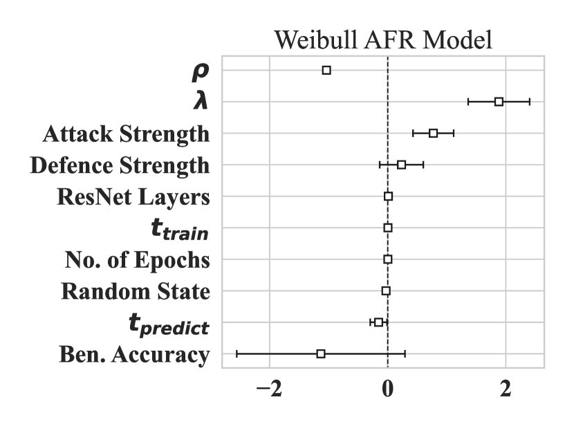
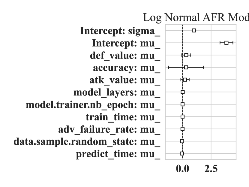
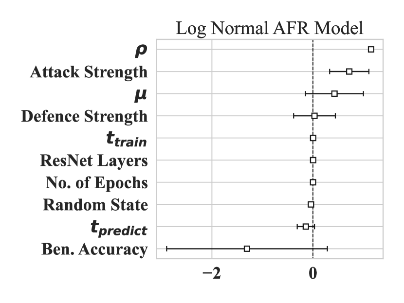
Figure 1: The covariate estimates accelerated failure time models where the parameters $\rho$, $h$, $\mu$, $\sigma$, $\alpha$, and $\beta$ represent the intercepts for those parameters as described in Sec. 3 for the Weibull, Log-Normal, and Log-Logistic AFR Models. The coefficients represent the log scale effect of the covariates on the failure rate. Additionally, $\lambda_{ben}$ refers to the benign accuracy (see Eq. 1) and $f_{adv.}$ refers to the adversarial hazard function (see: Eq. 6)

.

Table 1: Comparison of AFR Models on the CIFAR100 dataset.

Distribution	AIC	Concordance	BIC	Mean $S(t;\theta)$	Median $S(t;\theta)$
Weibull	5026.59	0.77	5026.59	578.43	79.44
Log-Normal	5038.16	0.79	5038.16	4736.64	73.43
Log-Logistic	5066.87	0.78	5066.87	–	78.79

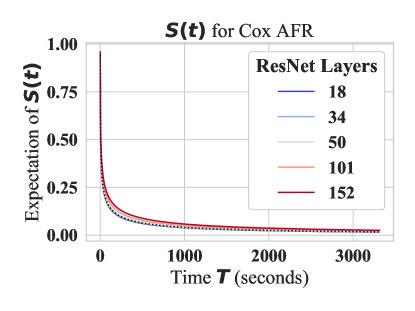
Figure 2: The survival curve over time as a function of the number of model layers for the highest scoring AFR model (the Log-Normal distribution). The partial effects plots of other models are included in the Appendix A, as the results were very similar.

7 Considerations

The proposed survival and cost analysis has some limitations that we have taken all efforts to minimize and/or mitigate. In order to minimize timing jitter, we measured the process time for a batch of samples and then assumed that the time per sample was the measured processor time divided by the number of samples. In order to examine a variety of different optimization critera for adversarial perturbations, we included several different attacks (see Sec. 5.4)—though the choice of attack is highly contextual. We must also note that none of these attacks are run-time optimal and are, at best, an underestimate of the true adversarial failure rate [Meyers et al., 2023]. Of course, further run-time optimizations are possible, but this would be beyond the scope of this paper. One such optimization is running evaluations on GPUs with a smaller physical bit-depth than a V100, since FSQ doesn’t seem to hinder the model significantly (see Fig. 3). This could yield a tremendous power savings over standard server-grade GPUs [Chou et al., 2023]. However, the goal of this work was not to produce a perfect measure of failure rate but to develop a technique for measuring and predicting the expected adversarial failure rate for a large number of proposed models and defences across a wide variety of attacks on a targeted piece of hardware.

8 Conclusion

Convolutional neural networks have shown to be widely applicable to a large number of fields when large amounts of labelled data are available. By examining the role of the attacks, defences, and model depth in the context of adversarial failure rate, we were able to build a reliable and effective modelling framework that applies accelerated failure rate models to deep neural networks. Through statistical analysis (see Eq. 1–8 and Tables 3& 4), we show that this method is both effective and data-agnostic. We use this model to demonstrate the efficacy of attack- and defence-tuning (see Fig. 1) to explore the relationships between accuracy and adversarial robustness (Fig. 4), showing that various model defences are ineffective on average and marginally better than the control at best. By measuring the cost-normalized failure rate (see Sec. 2.2 and Fig. 5), we show that robustness gains from deeper networks is driven by model latency more than inherent robustness (Fig. 1). Our methods can easily extend to any other arbitrary collection of model pre-processing, training, tuning, attack and/or deployment parameters. In short, we provide a rigorous way to compare not only the relative robustness of a model, but of its cost effectiveness in response to an attacker. Our measurements rigorously demonstrate that the depth of a Resnet architecture does little to guarantee robustness while the community trends towards larger models Desislavov et al. [2021], larger datasets Desislavov et al. [2021], Bailly et al. [2022], and increasingly marginal gains Sun et al. [2017].

Appendix A Appendix

In addition to the results on the CIFAR10 [Krizhevsky et al., 2009] dataset, presented in Section 6, we provide the same analysis for the MNIST [Deng, 2012] and CIFAR100 [Krizhevsky et al., 2009] datasets.

A.1 CIFAR100

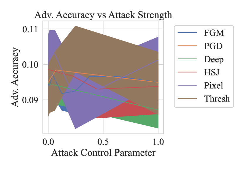
Figure 3: This depicts the benign (unperturbed) and adversarial (perturbed) accuracies across all defences attacks, and models. The left shows how the benign accuracy varies with the defence strength where the control parameter describes the number of layers. The right shows the adversarial accuracy as a function of attack strength, and the definition can be found in Eq. 1. The shaded areas reflect the 95% confidence intervals for performance across random configurations of the data for each tuned attack and model configuration.

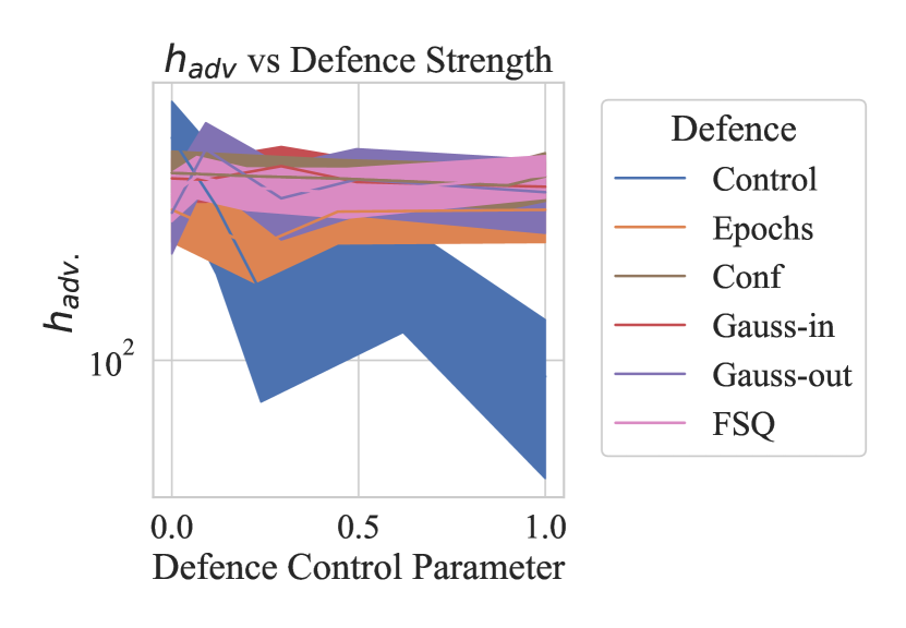
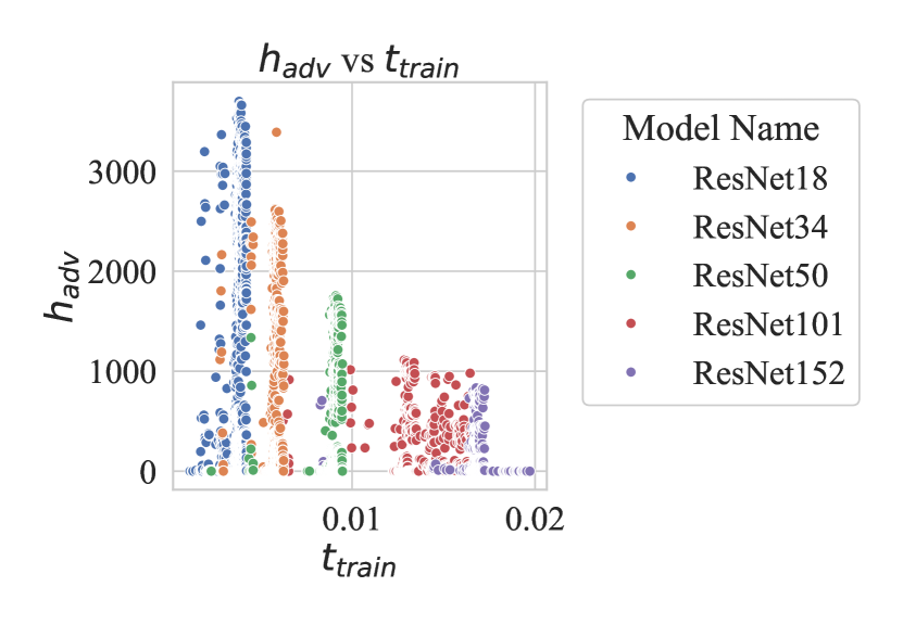
Figure 4: The left plot shows the adversarial failure rate (see Eq. 2) as a function of the defence strength where the control parameter represents the number of model layers. The shaded areas reflect the 95% confidence intervals for each tuned hyperparameter combination. The right plot depicts the adversarial failure rate as a function of training time and ResNet configuration.

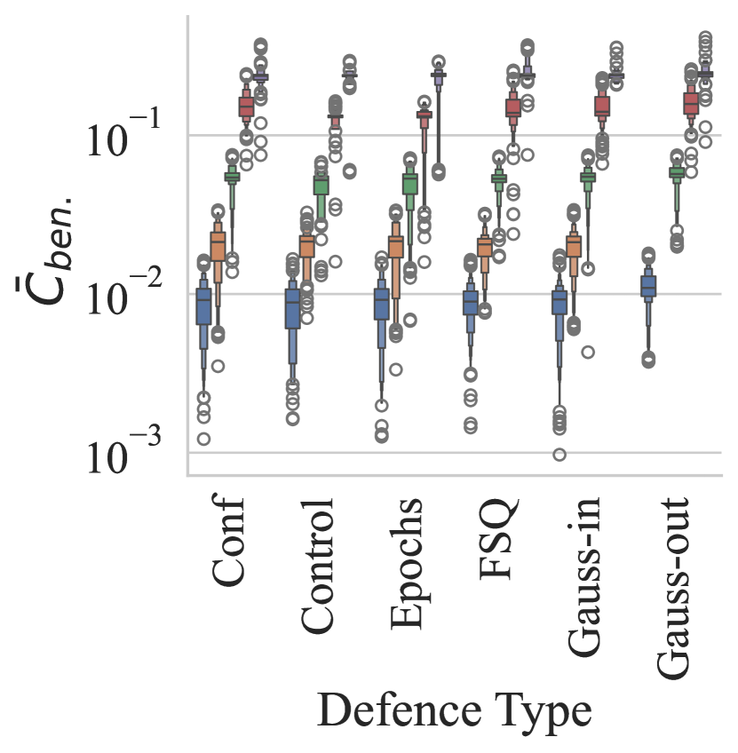
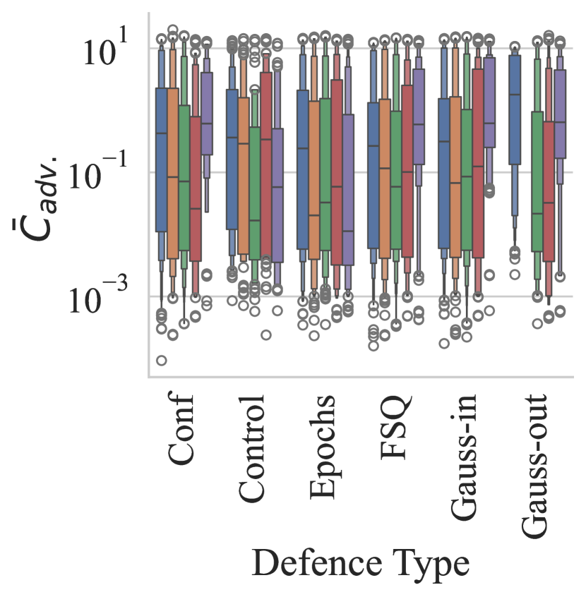
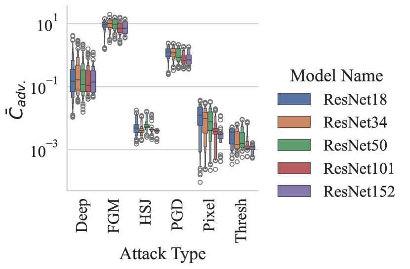
Figure 5: This figure depicts the cost-normalized adversarial failure rate (see Eq. 8) across a variety of defences and attacks, where training time (middle & right Figs.) and inference time (left figure) is a stand-in for cost (see Sec. 2.2). The violin plots reflect the 95% confidence intervals for each tuned hyperparameter combination. Outliers are indicated with a diamond.

Below, we present supplementary data for the CIFAR100 dataset in Figures 3- 5.

A.2 MNIST

Below, we present supplementary data for the CIFAR100 dataset in Figures 6- 11.

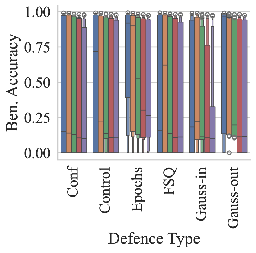
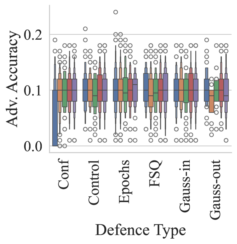
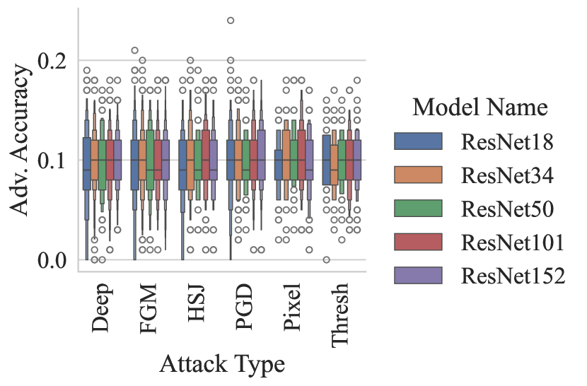
Figure 6: The adversarial accuracy across various attacks pictured on the x-axis and outlined in Section 5.4. The error bar reflects the 95% confidence interval for the adversarial accuracy across all examined samples.

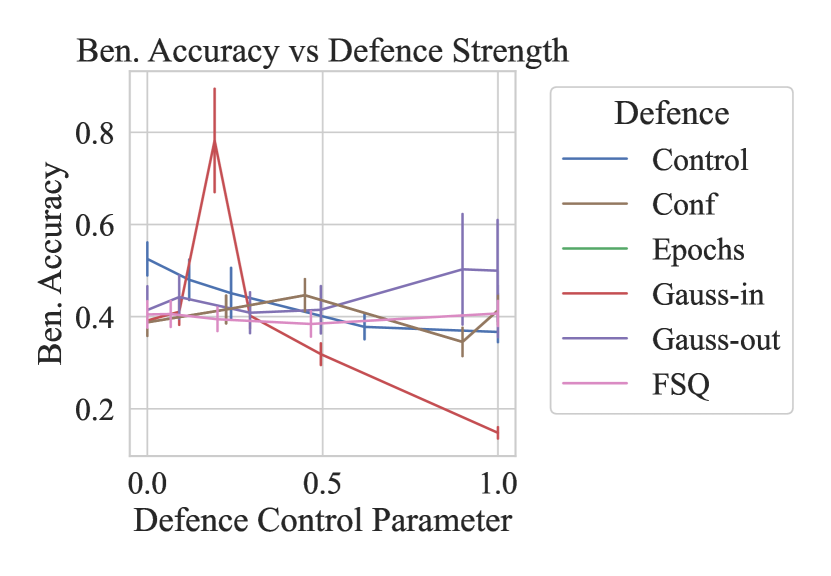
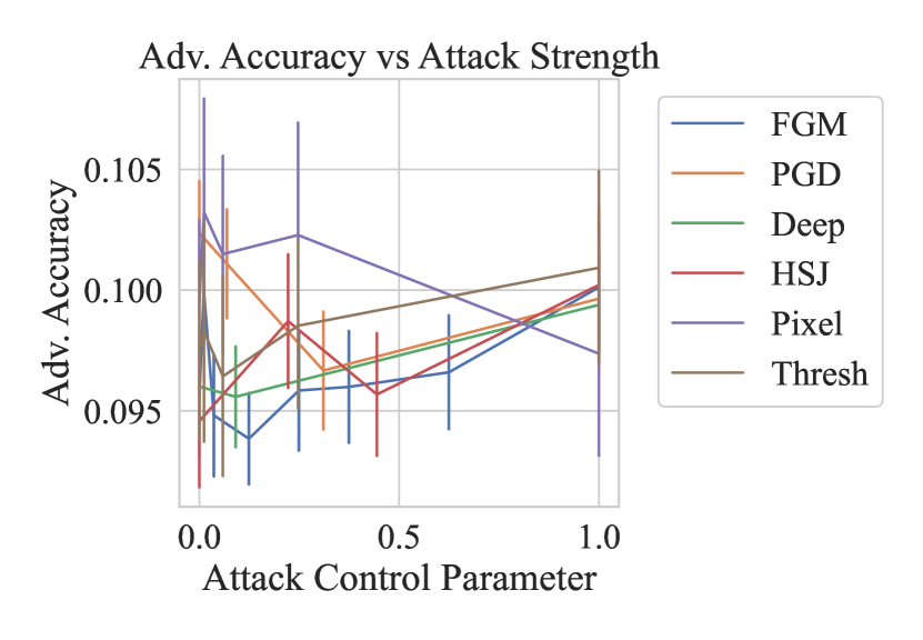
Figure 7: This depicts the benign (unperturbed) and adversarial (perturbed) failure rates across all defences attacks, and models. The left shows how the benign accuracy varies with the defence strength where the control parameter describes the number of layers. The right shows the adversarial accuracy as a function of attack strength.

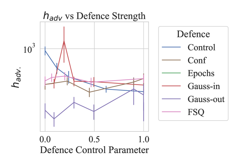
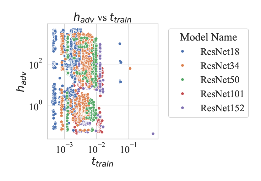
Figure 8: The left shows the adversarial failure rate as a function of the defence strength where the control parameter represents the number of model layers. The right depicts the adversarial failure rate as a function of training time and the ResNet configuration.

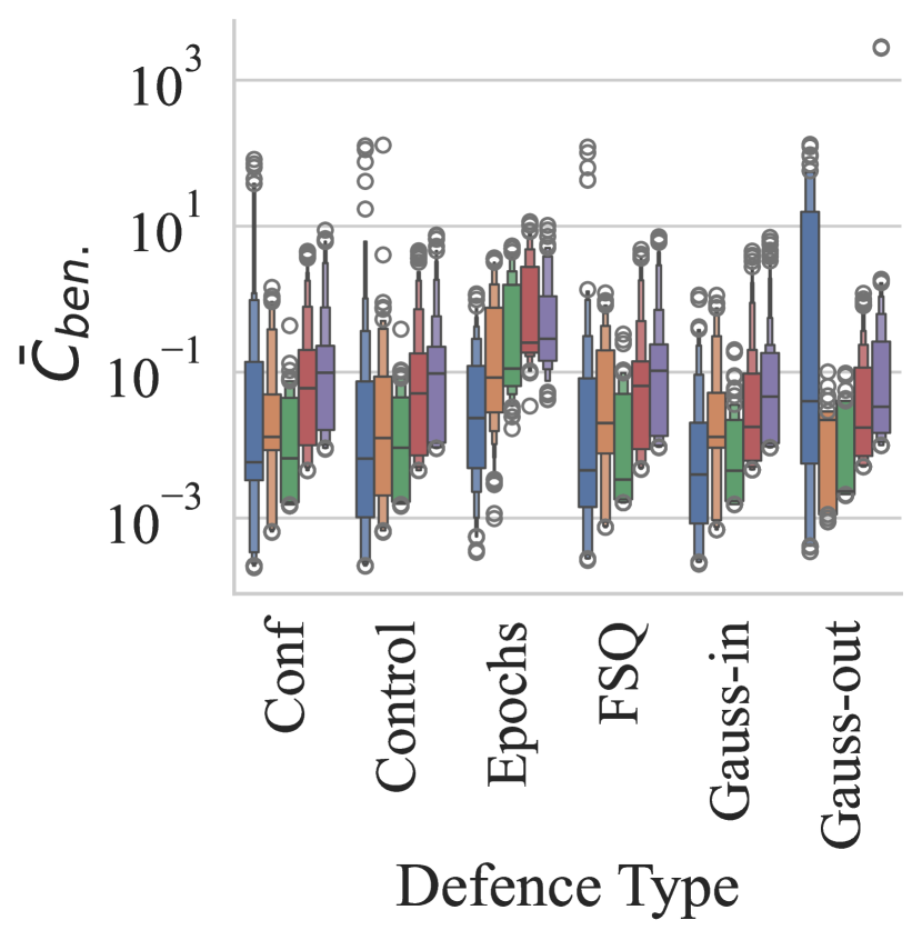
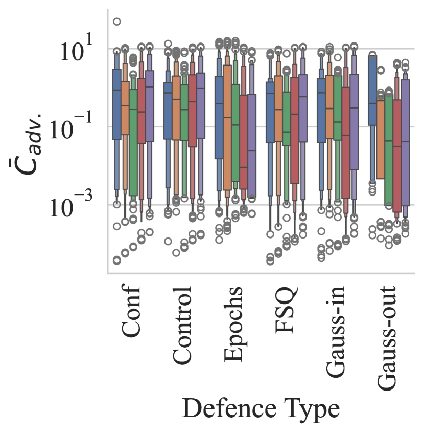
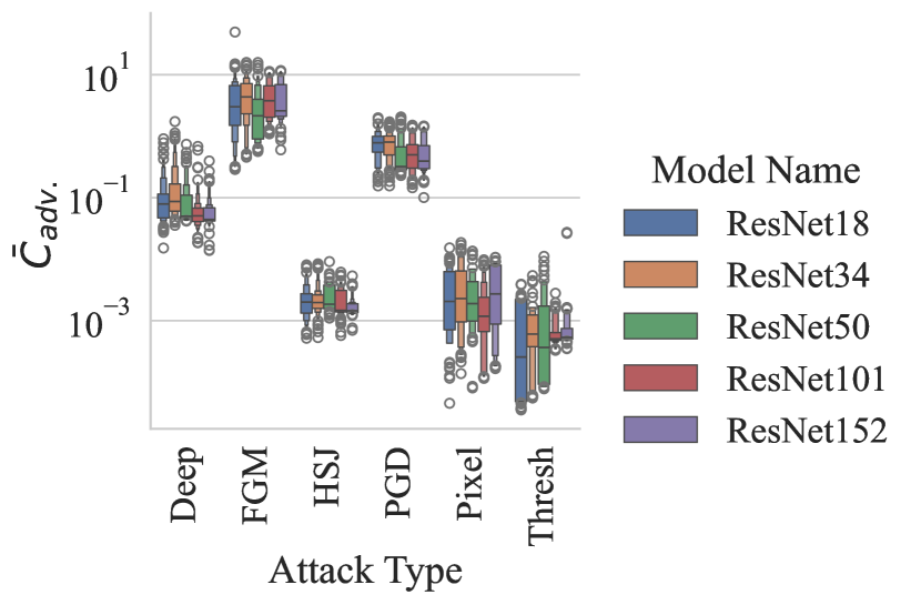
Figure 9: This figure depicts the cost-normalized adversarial failure rate across a variety of defences and attacks, where training time (middle & right Figs.) and inference time (left figure) is a stand-in for cost (see Section 2.2).

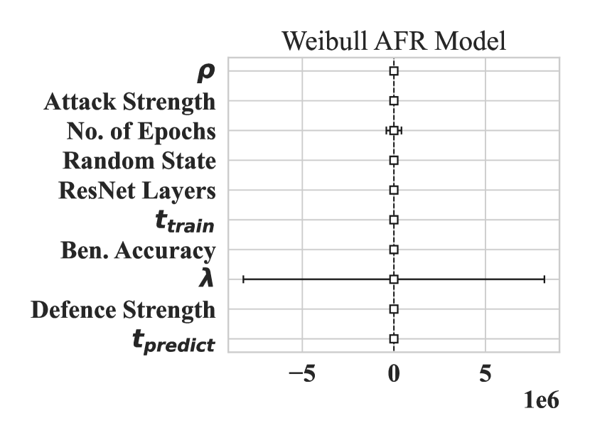
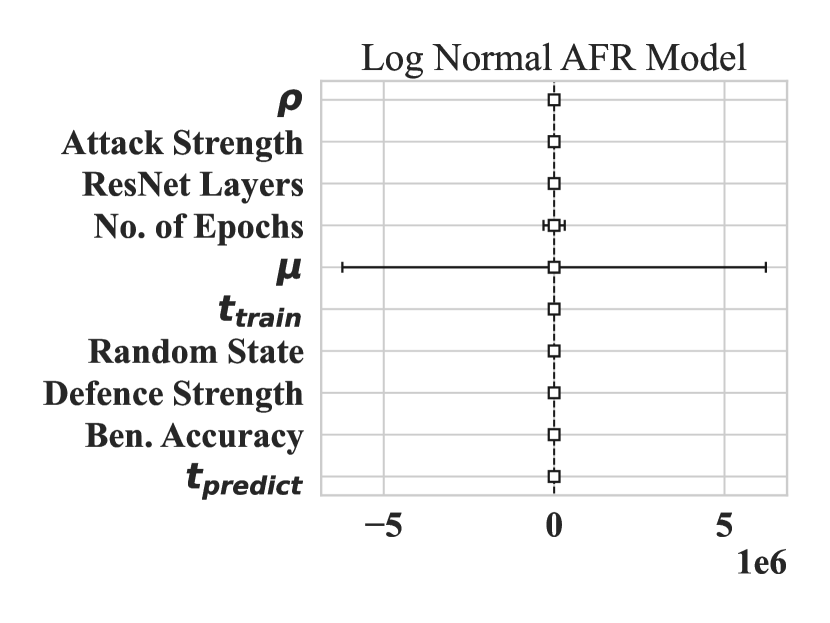
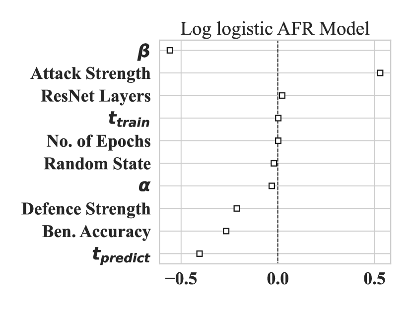
Figure 10: The covariate estimates accelerated failure time models where the parameters $\rho$, $\lambda$, $\mu$, $\sigma$, $\alpha$, and $\beta$ represent the intercepts for those parameters as described in Section 3 for the Weibull, Log-Normal, and Log-Logistic AFR Models. The coefficients represent the log scale effect of the covariates on the failure rate.

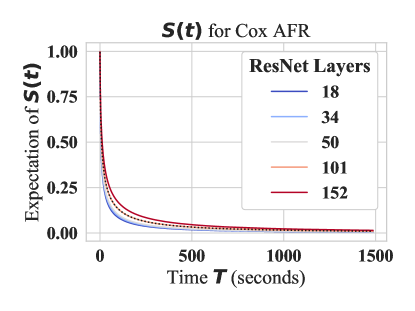
Figure 11: This figure depicts the survival curve over time as a function of the number of model layers for the highest scoring model (the Log-Normal distribution). The partial effects plots of other models were excluded for space reasons, but the results were nearly identical.

A.3 CIFAR10

Below, we present supplementary data for the CIFAR100 dataset in Figures 12- 17.

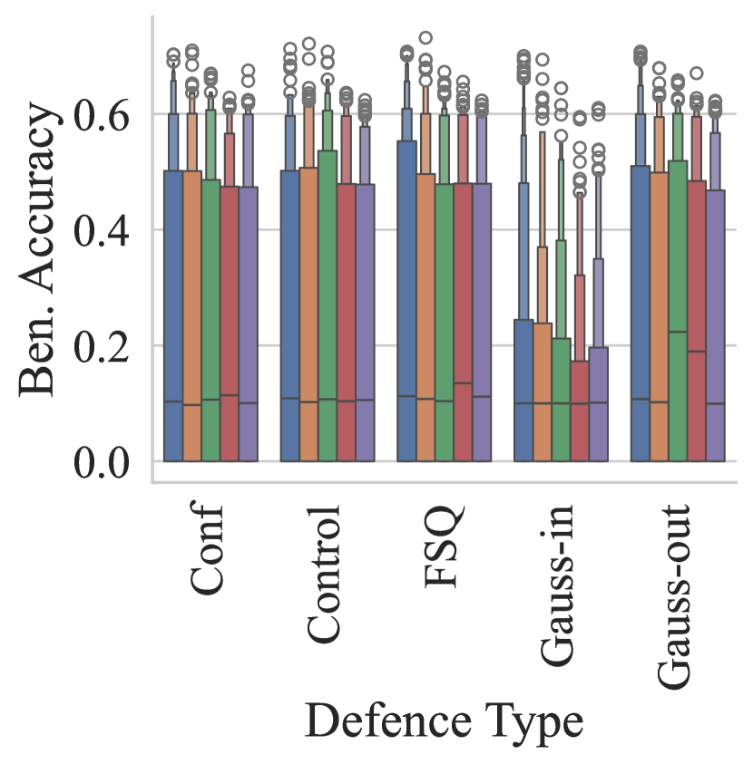
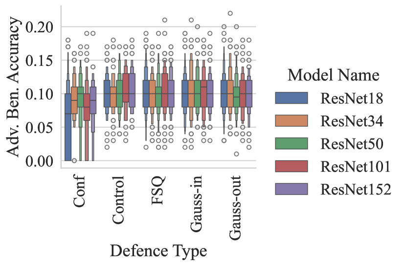
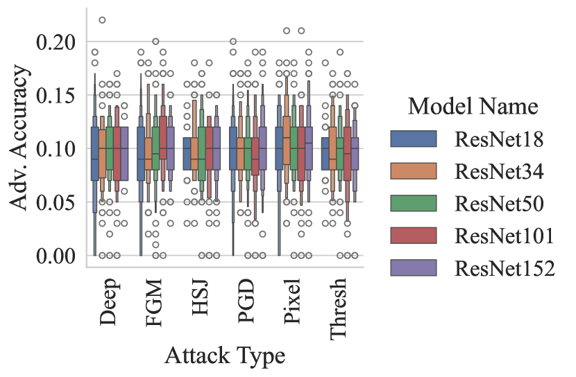
Figure 12: The adversarial accuracy across various attacks pictured on the x-axis and outlined in Section 5.4. The error bar reflects the 95% confidence interval for the adversarial accuracy across all examined samples.

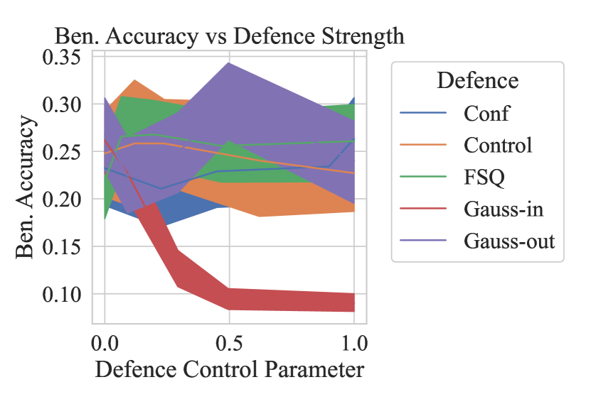
Figure 13: This depicts the benign (unperturbed) and adversarial (perturbed) failure rates across all defences attacks, and models. The left shows how the benign accuracy varies with the defence strength where the control parameter describes the number of layers. The right shows the adversarial accuracy as a function of attack strength.

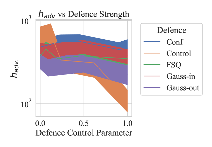
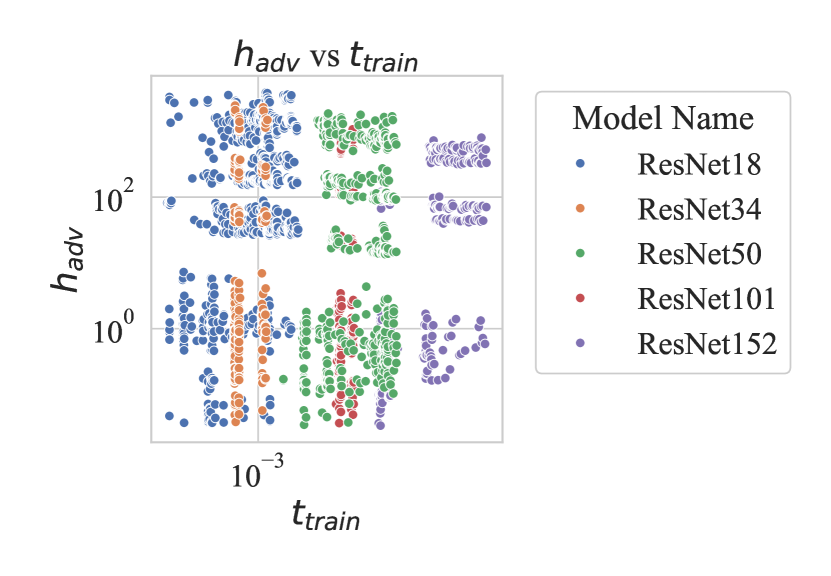
Figure 14: The left shows the adversarial failure rate as a function of the defence strength where the control parameter represents the number of model layers. The right depicts the adversarial failure rate as a function of training time and the ResNet configuration.

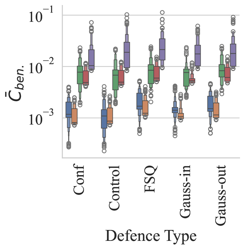
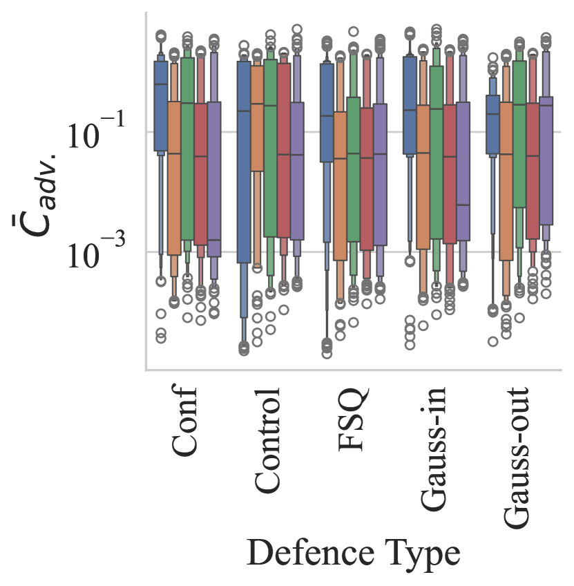
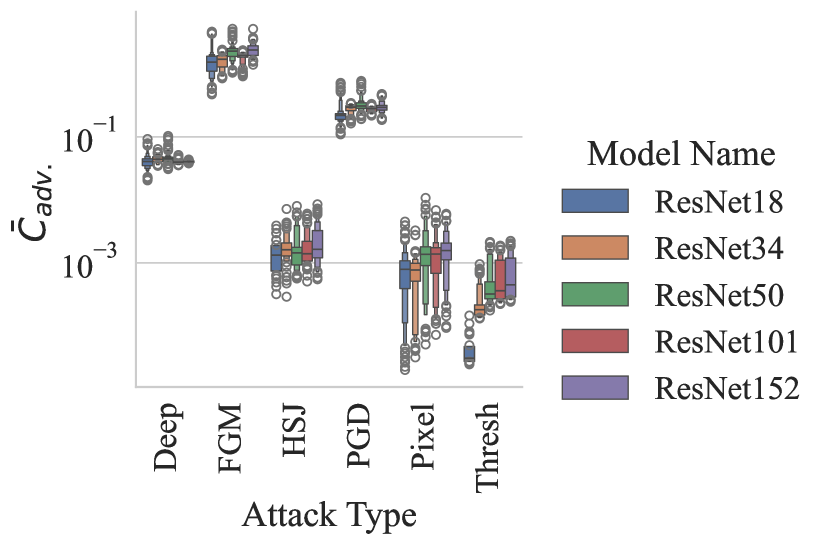
Figure 15: This figure depicts the cost-normalized adversarial failure rate across a variety of defences and attacks, where training time (middle & right Figs.) and inference time (left figure) is a stand-in for cost (see Section 2.2).

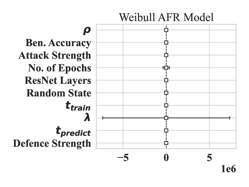
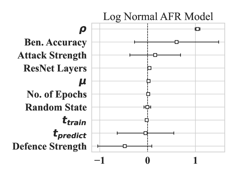
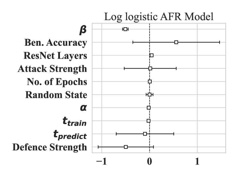
Figure 16: The covariate estimates accelerated failure time models where the parameters $\rho$, $\lambda$, $\mu$, $\sigma$, $\alpha$, and $\beta$ represent the intercepts for those parameters as described in Section 3 for the Weibull, Log-Normal, and Log-Logistic AFR Models. The coefficients represent the log scale effect of the covariates on the failure rate.

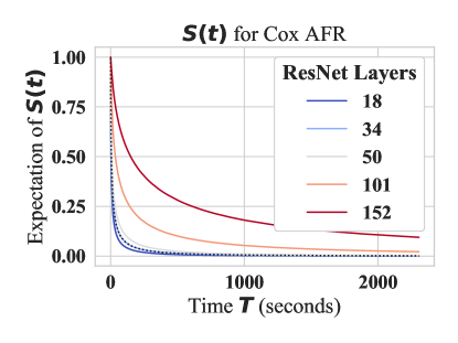
Figure 17: This figure depicts the survival curve over time as a function of the number of model layers for the highest scoring model (the Log-Normal distribution). The partial effects plots of other models were excluded for space reasons, but the results were nearly identical.

A.4 Comparison of datasets

Tables 2-4 compare the efficacy of the AFR technique across datasets.

Table 2: Comparison of AFR Models on the CIFAR100 dataset.

Distribution	AIC	Concordance	BIC	Mean $S(t;\theta)$	Median $S(t;\theta)$
Weibull	5026.59	0.77	5026.59	578.43	79.44
Log-Normal	5038.16	0.79	5038.16	4736.64	73.43
Log-Logistic	5066.87	0.78	5066.87	–	78.79

Table 3: Comparison of AFR Models on the CIFAR10 dataset.

Distribution	AIC	Concordance	BIC	Mean $S(t;\theta)$	Median $S(t;\theta)$
Weibull	4464.42	0.84	4464.42	64.30	4.62
Log-Logistic	4258.52	0.83	4258.52	–	2.70
Log-Normal	4242.50	0.84	4242.50	66.49	3.59

Table 4: Comparison of AFR Models on the MNIST dataset.

Distribution	AIC	Concordance	BIC	Mean $S(t;\theta)$	Median $S(t;\theta)$
Weibull	6023.09	0.79	6023.09	55.49	6.80
Log-Logistic	5856.06	0.85	5856.06	–	5.18
Log-Normal	5808.19	0.84	5808.19	69.42	5.72

References

- Akiba et al. [2019] Takuya Akiba, Shotaro Sano, Toshihiko Yanase, Takeru Ohta, and Masanori Koyama. Optuna: A next-generation hyperparameter optimization framework. In Proceedings of the 25th ACM SIGKDD international conference on knowledge discovery & data mining, pages 2623–2631, 2019.
- Arp et al. [2022] Daniel Arp, Erwin Quiring, Feargus Pendlebury, Alexander Warnecke, Fabio Pierazzi, Christian Wressnegger, Lorenzo Cavallaro, and Konrad Rieck. Dos and don’ts of machine learning in computer security. In 31st USENIX Security Symposium (USENIX Security 22), pages 3971–3988, 2022.
- Bailly et al. [2022] Alexandre Bailly, Corentin Blanc, Élie Francis, Thierry Guillotin, Fadi Jamal, Béchara Wakim, and Pascal Roy. Effects of dataset size and interactions on the prediction performance of logistic regression and deep learning models. Computer Methods and Programs in Biomedicine, 213:106504, 2022.
- Biggio et al. [2013a] Battista Biggio, Igino Corona, Davide Maiorca, Blaine Nelson, Nedim Šrndić, Pavel Laskov, Giorgio Giacinto, and Fabio Roli. Evasion attacks against machine learning at test time. pages 387–402, 2013a.
- Biggio et al. [2013b] Battista Biggio, Blaine Nelson, and Pavel Laskov. Poisoning Attacks against Support Vector Machines. arXiv:1206.6389 [cs, stat], March 2013b. URL http://arxiv.org/abs/1206.6389.
- Bradburn et al. [2003] Mike J Bradburn, Taane G Clark, Sharon B Love, and Douglas Graham Altman. Survival analysis part ii: multivariate data analysis–an introduction to concepts and methods. British journal of cancer, 89(3):431–436, 2003.
- Brown et al. [2017] Tom B Brown, Dandelion Mané, Aurko Roy, Martín Abadi, and Justin Gilmer. Adversarial patch. arXiv:1712.09665, 2017.
- Carlini and Wagner [2017] Nicholas Carlini and David Wagner. Towards evaluating the robustness of neural networks. pages 39–57, 2017.
- Chakraborty et al. [2018] Anirban Chakraborty, Manaar Alam, Vishal Dey, Anupam Chattopadhyay, and Debdeep Mukhopadhyay. Adversarial attacks and defences: A survey. arXiv:1810.00069 [cs, stat], 2018.
- Chen et al. [2020] Jianbo Chen, Michael I Jordan, and Martin J Wainwright. HopSkipJumpAttack: A query-efficient decision-based attack. In IEEE symposium on security and privacy (sp), pages 1277–1294. IEEE, 2020.
- Chen et al. [2021] Li Chen, Jun Xiao, Pu Zou, and Haifeng Li. Lie to me: A soft threshold defense method for adversarial examples of remote sensing images. IEEE Geoscience and Remote Sensing Letters, pages 1–5, 2021. doi: 10.1109/LGRS.2021.3096244.
- Choquette-Choo et al. [2021] Christopher A Choquette-Choo, Florian Tramer, Nicholas Carlini, and Nicolas Papernot. Label-only membership inference attacks. In International conference on machine learning, pages 1964–1974. PMLR, 2021.
- Chou et al. [2023] Po-Hsuan Chou, Chao Wang, and Chih-Shuo Mei. Applicability of deep learning model trainings on embedded gpu devices: An empirical study. In 2023 12th Mediterranean Conference on Embedded Computing (MECO), pages 1–4. IEEE, 2023.
- Croce and Hein [2020] Francesco Croce and Matthias Hein. Reliable evaluation of adversarial robustness with an ensemble of diverse parameter-free attacks. pages 2206–2216, 2020.
- Davidson-Pilon [2019] Cameron Davidson-Pilon. lifelines: survival analysis in python. Journal of Open Source Software, 4(40):1317, 2019. doi: 10.21105/joss.01317. URL https://doi.org/10.21105/joss.01317.
- Deb et al. [2002] Kalyanmoy Deb, Amrit Pratap, Sameer Agarwal, and TAMT Meyarivan. A fast and elitist multiobjective genetic algorithm: Nsga-ii. IEEE transactions on evolutionary computation, 6(2):182–197, 2002.
- Deng [2012] Li Deng. The mnist database of handwritten digit images for machine learning research. IEEE Signal Processing Magazine, 29(6):141–142, 2012.
- Desislavov et al. [2021] Radosvet Desislavov, Fernando Martínez-Plumed, and José Hernández-Orallo. Compute and energy consumption trends in deep learning inference. arXiv:2109.05472, 2021.
- Dohmatob [2019] Elvis Dohmatob. Generalized No Free Lunch Theorem for Adversarial Robustness. In Proceedings of the 36th International Conference on Machine Learning, volume 97 of PMLR, 2019.
- dvc.org [2023] dvc.org. DVC–Data Version Control. Github, 2023. URL https://github.com/iterative/dvc.org.
- Erickson et al. [2017] Bradley J Erickson, Panagiotis Korfiatis, Zeynettin Akkus, and Timothy L Kline. Machine learning for medical imaging. Radiographics, 37(2):505–515, 2017.
- Goodfellow et al. [2014] Ian J Goodfellow, Jonathon Shlens, and Christian Szegedy. Explaining and harnessing adversarial examples. arXiv:1412.6572, 2014.
- He et al. [2016] Kaiming He, Xiangyu Zhang, Shaoqing Ren, and Jian Sun. Deep residual learning for image recognition. In Proceedings of the IEEE conference on computer vision and pattern recognition, pages 770–778, 2016.
- Hochreiter [1998] Sepp Hochreiter. The vanishing gradient problem during learning recurrent neural nets and problem solutions. International Journal of Uncertainty, Fuzziness and Knowledge-Based Systems, 6(02):107–116, 1998.
- Jahan et al. [2016] Ali Jahan, Kevin L Edwards, and Marjan Bahraminasab. Multi-criteria decision analysis for supporting the selection of engineering materials in product design. Butterworth-Heinemann, 2016.
- Kamal [2017] Parves Kamal. A study on the security of password hashing based on gpu based, password cracking using high-performance cloud computing. 2017.
- Kleinbaum and Klein [1996] David G Kleinbaum and Mitchel Klein. Survival analysis a self-learning text. Springer, 1996.
- Koay et al. [2023] Abigail MY Koay, Ryan K L Ko, Hinne Hettema, and Kenneth Radke. Machine learning in industrial control system (ics) security: current landscape, opportunities and challenges. Journal of Intelligent Information Systems, 60(2):377–405, 2023.
- Kotyan and Vargas [2022] Shashank Kotyan and Danilo Vasconcellos Vargas. Adversarial robustness assessment: Why in evaluation both and attacks are necessary. PloS one, 17(4):e0265723, 2022.
- Krizhevsky et al. [2009] Alex Krizhevsky, Geoffrey Hinton, et al. Learning multiple layers of features from tiny images. 2009.
- Lachin [1981] John M Lachin. Introduction to sample size determination and power analysis for clinical trials. Controlled clinical trials, 2(2):93–113, 1981.
- Lambert et al. [2004] Philippe Lambert, Dave Collett, Alan Kimber, and Rachel Johnson. Parametric accelerated failure time models with random effects and an application to kidney transplant survival. Statistics in medicine, 23(20):3177–3192, 2004.
- Lawless et al. [1995] Jerry Lawless, Joan Hu, and Jin Cao. Methods for the estimation of failure distributions and rates from automobile warranty data. Lifetime Data Analysis, 1:227–240, 1995.
- Lecuyer et al. [2019] Mathias Lecuyer, Vaggelis Atlidakis, Roxana Geambasu, Daniel Hsu, and Suman Jana. Certified robustness to adversarial examples with differential privacy. In 2019 IEEE Symposium on Security and Privacy (SP), pages 656–672, 2019.
- Leurent and Peyrin [2020] Gaëtan Leurent and Thomas Peyrin. SHA-1 is a shambles: First Chosen-Prefix collision on SHA-1 and application to the PGP web of trust. In 29th USENIX security symposium (USENIX security 20), pages 1839–1856, 2020.
- Li and Zhang [2021] Zheng Li and Yang Zhang. Membership leakage in label-only exposures. In Proceedings of the 2021 ACM SIGSAC Conference on Computer and Communications Security, pages 880–895, 2021.
- Liu et al. [2013] Qiang Liu, Azianti Ismail, and Won Jung. Development of accelerated failure-free test method for automotive alternator magnet. Journal of the Society of Korea Industrial and Systems Engineering, 36(4):92–99, 2013.
- Longato et al. [2020] Enrico Longato, Martina Vettoretti, and Barbara Di Camillo. A practical perspective on the concordance index for the evaluation and selection of prognostic time-to-event models. Journal of biomedical informatics, 108:103496, 2020.
- Ma et al. [2020] Xingjun Ma, Linxi Jiang, Hanxun Huang, Zejia Weng, James Bailey, and Yu-Gang Jiang. Imbalanced gradients: A subtle cause of overestimated adversarial robustness. arXiv:2006.13726, 2020.
- Madry et al. [2017] Aleksander Madry, Aleksandar Makelov, Ludwig Schmidt, Dimitris Tsipras, and Adrian Vladu. Towards deep learning models resistant to adversarial attacks. arXiv:1706.06083, 2017.
- Maheshwari et al. [2018] Apoorv Maheshwari, Navindran Davendralingam, and Daniel A DeLaurentis. A comparative study of machine learning techniques for aviation applications. In 2018 Aviation Technology, Integration, and Operations Conference, page 3980, 2018.
- International Electrotechnical Commission [2006] International Electrotechnical Commission. IEC 62304 Medical Device Software - Software Life Cycle Processes. International Electrotechnical Commission, 2nd edition, 2006.
- International Electrotechnical Commission [2010] International Electrotechnical Commission. IEC 61508 Safety and Functional Safety. International Electrotechnical Commission, 2nd edition, 2010.
- International Standards Organization [2018] International Standards Organization. ISO 26262-1:2011, road vehicles — functional safety. https://www.iso.org/standard/43464.html (visited 2022-04-20), 2018.
- Meeker et al. [1998] William Q Meeker, Luis A Escobar, and C Joseph Lu. Accelerated degradation tests: modeling and analysis. Technometrics, 40(2):89–99, 1998.
- Mery et al. [2016] Domingo Mery, Erick Svec, Marco Arias, Vladimir Riffo, Jose M Saavedra, and Sandipan Banerjee. Modern computer vision techniques for x-ray testing in baggage inspection. IEEE Transactions on Systems, Man, and Cybernetics: Systems, 47(4):682–692, 2016.
- Meyers et al. [2023] Charles Meyers, Tommy Löfstedt, and Erik Elmroth. Safety-critical computer vision: An empirical survey of adversarial evasion attacks and defenses on computer vision systems. Springer Artificial Intelligence Review, 2023.
- Moosavi-Dezfooli et al. [2016] Seyed-Mohsen Moosavi-Dezfooli, Alhussein Fawzi, and Pascal Frossard. Deepfool: a simple and accurate method to fool deep neural networks. In Proceedings of the IEEE conference on computer vision and pattern recognition, pages 2574–2582, 2016.
- Nicolae et al. [2018] Maria-Irina Nicolae, Mathieu Sinn, Minh Ngoc Tran, Beat Buesser, Ambrish Rawat, Martin Wistuba, Valentina Zantedeschi, Nathalie Baracaldo, Bryant Chen, Heiko Ludwig, Ian Molloy, and Ben Edwards. Adversarial robustness toolbox v1.2.0. CoRR, 1807.01069, 2018. URL https://arxiv.org/pdf/1807.01069.
- Orekondy et al. [2019] Tribhuvanesh Orekondy, Bernt Schiele, and Mario Fritz. Knockoff nets: Stealing functionality of black-box models. In Proceedings of the IEEE/CVF conference on computer vision and pattern recognition, pages 4954–4963, 2019.
- Rolnick and Tegmark [2017] David Rolnick and Max Tegmark. The power of deeper networks for expressing natural functions. arXiv preprint arXiv:1705.05502, 2017.
- Saha et al. [2020] Aniruddha Saha, Akshayvarun Subramanya, and Hamed Pirsiavash. Hidden trigger backdoor attacks. In Proceedings of the AAAI conference on artificial intelligence, volume 34, pages 11957–11965, 2020.
- Santos et al. [2021] Pablo Millán Santos, BR Manoj, Meysam Sadeghi, and Erik G Larsson. Universal adversarial attacks on neural networks for power allocation in a massive mimo system. IEEE Wireless Communications Letters, 11(1):67–71, 2021.
- Schmoor et al. [2000] Claudia Schmoor, Willi Sauerbrei, and Martin Schumacher. Sample size considerations for the evaluation of prognostic factors in survival analysis. Statistics in medicine, 19(4):441–452, 2000.
- Simonyan and Zisserman [2014] Karen Simonyan and Andrew Zisserman. Very deep convolutional networks for large-scale image recognition. arXiv preprint arXiv:1409.1556, 2014.
- Stoica and Selen [2004] Petre Stoica and Yngve Selen. Model-order selection: a review of information criterion rules. IEEE Signal Processing Magazine, 21(4):36–47, 2004.
- Sun et al. [2017] Chen Sun, Abhinav Shrivastava, Saurabh Singh, and Abhinav Gupta. Revisiting unreasonable effectiveness of data in deep learning era. In Proceedings of the IEEE international conference on computer vision, pages 843–852, 2017.
- Taddy [2019] Matt Taddy. Business data science: Combining machine learning and economics to optimize, automate, and accelerate business decisions. McGraw-Hill Education, 2019.
- tommyod [2020] tommyod. paretoset, 2020.
- Travaini et al. [2022] Guido Vittorio Travaini, Federico Pacchioni, Silvia Bellumore, Marta Bosia, and Francesco De Micco. Machine learning and criminal justice: A systematic review of advanced methodology for recidivism risk prediction. International journal of environmental research and public health, 19(17):10594, 2022.
- Vapnik et al. [1994] Vladimir Vapnik, Esther Levin, and Yann Le Cun. Measuring the vc-dimension of a learning machine. Neural computation, 6(5):851–876, 1994.
- Xu et al. [2017] Weilin Xu, David Evans, and Yanjun Qi. Feature squeezing: Detecting adversarial examples in deep neural networks. arXiv:1704.01155, 2017.
- Yadan [2019] Omry Yadan. Hydra - a framework for elegantly configuring complex applications. Github, 2019. URL https://github.com/facebookresearch/hydra.
- Zantedeschi et al. [2017] Valentina Zantedeschi, Maria-Irina Nicolae, and Ambrish Rawat. Efficient defenses against adversarial attacks. In Proceedings of the 10th ACM Workshop on Artificial Intelligence and Security, AISec ’17, page 39–49, New York, NY, USA, 2017. Association for Computing Machinery. ISBN 9781450352024. doi: 10.1145/3128572.3140449. URL https://doi.org/10.1145/3128572.3140449.