The $M_{\rm BH}-M_{*}$ relation up to $z\sim 2$ through decomposition of COSMOS-Web NIRCam images

Abstract

Our knowledge of relations between supermassive black holes and their host galaxies at $z\gtrsim 1$ is still limited, even though being actively sought out to $z\sim 6$. Here, we use the high resolution and sensitivity of JWST to measure the host galaxy properties for 61 X-ray-selected type-I AGNs at $0.7<z<2.5$ with rest-frame optical/near-infrared imaging from COSMOS-Web and PRIMER. Black hole masses ($\log\left(M_{\rm BH}/M_{\odot}\right)\sim 7.5-9.5$) are available from previous spectroscopic campaigns. We extract the host galaxy components from four NIRCam broadband images and the HST/ACS F814W image by applying a 2D image decomposition technique. We detect the host galaxy for $\sim 90\%$ of the sample after subtracting the unresolved AGN emission. With host photometry free of AGN emission, we determine the stellar mass of the host galaxies to be $\log\left(M_{*}/M_{\odot}\right)\sim 10-11.5$ through SED fitting and measure the evolution of the mass relation between SMBHs and their host galaxies. Considering selection biases and measurement uncertainties, we find that the $M_{\mathrm{BH}}/M_{*}$ ratio evolves as $\left(1+z\right)^{0.37_{-0.60}^{+0.35}}$ thus remains essentially constant or exhibits mild evolution up to $z\sim 2.5$. We also see an amount of scatter ($\sigma_{\mu}=0.28\pm 0.13$) is similar to the local relation and consistent with low-$z$ studies; this appears to not rule out non-causal cosmic assembly where mergers contribute to the statistical averaging towards the local relation. We highlight improvements to come with larger samples from JWST and, particularly, Euclid, which will exceed the statistical power of wide and deep surveys such as Subaru Hyper Suprime-Cam.

1 Introduction

With our understanding that galaxies grow by increasing their stellar mass through mergers and in situ star formation from gas accretion, there are still many unresolved questions in galaxy evolution. One of the most important challenges in galaxy formation is understanding the physical processes that relate the growth of supermassive black holes (SMBHs) alongside the growth of the galaxies that harbor them. Observational studies, mainly in the local universe, have unveiled tight correlations between the mass of SMBHs ($M_{\rm BH}$) and the physical properties of their host galaxies, such as stellar velocity dispersion $\sigma_{*}$ and stellar mass $M_{*}$ (Magorrian et al., 1998; Ferrarese & Merritt, 2000; Marconi & Hunt, 2003; Häring & Rix, 2004; Gültekin et al., 2009; Graham et al., 2011; Beifiori et al., 2012; Kormendy & Ho, 2013; Reines & Volonteri, 2015). How and through what physical processes such a tight relation is formed is still unclear, and the origin of the mass relation can shed light on the evolution history of not only SMBHs but also galaxies.

A widely considered scenario, in answer to this question, is a co-evolution scheme, where galaxies and black holes mutually increase their mass at a correlated pace. As a potential physical cause for a co-evolution scenario, some studies implement active galactic nuclei (AGN) feedback, where the energy released from AGNs heats the gas and controls star formation or gas accretion through radio jets or an AGN winds (e.g. Springel et al., 2005; Di Matteo et al., 2008; Hopkins et al., 2008; Fabian, 2012; DeGraf et al., 2015; Harrison, 2017). Additionally, studies support a common gas supply simultaneously fueling both SMBHs and their host galaxies by increasing the BH accretion rate and star formation rate (SFR, Cen, 2015; Menci et al., 2016). On the other hand, others have shown that, even in the absence of a close physical connection between SMBHs and host galaxies, the mass relation can be achieved through a non-casual connection; major mergers have averaged the mass relation statistically (cosmic averaging scenario; Peng, 2007; Hirschmann et al., 2010; Jahnke & Macciò, 2011).

To unravel the cause of the mass relation, an effective approach is observing the relation between $M_{\rm BH}$ and $M_{*}$ throughout cosmic history. With such observations, we can directly determine whether the relation in the local universe, both its ratio and dispersion, evolves with redshift. Then, comparisons of the observational results with simulations (e.g., Ding et al., 2020; Habouzit et al., 2021; Ding et al., 2022b) based on various physical models can allow us to discuss the physical processes that establish the galaxy-BH relations and further constrain the physics of black hole formation and galaxy evolution.

Before the advent of James Webb Space Telescope (JWST), statistical studies using 2D image decomposition analyses were conducted using images obtained by Hubble Space Telescope (HST) (e.g., Peng et al., 2006; Jahnke et al., 2009; Bennert et al., 2011a; Cisternas et al., 2011; Simmons et al., 2011, 2012; Schramm & Silverman, 2013; Mechtley et al., 2016; Ding et al., 2020; Bennert et al., 2021; Li et al., 2023b) and ground-based telescopes including Subaru’s Hyper Suprime-Cam (HSC) (Ishino et al., 2020; Li et al., 2021), and Pan-STARRS1 (PS1) (Zhuang & Ho, 2023). In summary, these studies have concluded that the relation between $M_{\rm BH}$ and $M_{*}$ does not evolve with redshift at $z\lesssim 2$. However, studies using a large statistical and universal sample have yet to be achieved at $z>1$. At these redshifts, we can obtain information longer than the 4000 Å break to constrain $M_{*}$ from observations at near-infrared wavelengths. However, there are a limited number of previous studies using near-infrared data at $z\gtrsim 1$ (e.g., Jahnke et al., 2009; Simmons et al., 2012; Mechtley et al., 2016; Ding et al., 2020, utilizing HST/NICMOS or HST/WFC3). Other studies also studied statistical AGN samples using spectral energy distribution (SED) fitting based 1D decomposition method (e.g., Merloni et al., 2010; Sun et al., 2015; Suh et al., 2020).

JWST is now revolutionizing the field of AGN - host galaxy relations up to $z\sim 6$ and beyond based on its high spatial resolution and unprecedented sensitivity. For instance, Ding et al. (2022a) applied a 2D decomposition analysis on early JWST NIRCam data from CEERS that successfully detected the host galaxies of five quasars at $z\sim 1.6-3.5$ from the SDSS DR17Q catalog (Lyke et al., 2020). They also succeeded in detecting clear substructure and performed pixel-by-pixel SED fitting for one of the five targets, SDSSJ1420+5300A, at $z\sim 1.6$. Other studies have also performed 2D decompositions of AGN host galaxies using JWST imaging; for instance, Li et al. (2023a) have analyzed a galaxy that is one of the most promising candidates for having a recoiling SMBH ($z\sim 0.36$) while Kocevski et al. (2023) present the host properties of five X-ray-luminous AGNs ($3<z<5$) in CEERS. Zhang et al. (2023) also utilized JWST NIRCam data to assess the validity of $M*$ estimated from 1D decomposition (spectrum-based) method for the HETDEX type-I AGNs ($2<z<2.5$).

At $z>6$, Ding et al. (2023) conducted decomposition analysis of two low-luminosity quasars, thus representing the highest-redshift record for detection of host stellar emission. They suggest that $z\sim 6$ low luminosity quasars have a mass relation consistent with the local relation after considering selection biases and measurement uncertainties, albeit with a small sample. Equally remarkable, JWST studies of high-$z$ AGNs are revealing a higher abundance of lower mass black holes that are actively accreting within very dusty and compact galaxies (Onoue et al., 2023; Kocevski et al., 2023; Matthee et al., 2023; Harikane et al., 2023; Maiolino et al., 2023; Greene et al., 2023). However, in general, the sample sizes of these high-$z$ AGNs and the accuracy of $M_{*}$ estimation are still limited. Therefore, the redshift evolution of the mass relation remains highly uncertain.

Therefore, as an important next step to investigate the evolution of the mass relation, we perform a 2D decomposition analysis with JWST/NIRCam data for a sample whose redshift range significantly improves upon what was statistically analyzed before the JWST era, further bridging the gap between low-$z$ statistical and limited high-$z$ studies. We use a sample larger than previous studies using JWST, and that reaches up to $z\sim 2-3$ when AGN and star formation activities peaked in cosmic history. With NIRCam images of $N=61$ AGNs in COSMOS-Web (Casey et al., 2023) and PRIMER-COSMOS, we conduct 2D decomposition analyses and then statistically discuss the evolution of the $M_{BH}-M_{*}$ relation with consideration of the selection bias and measurement uncertainty (Lauer et al., 2007; Shen & Kelly, 2010; Schulze & Wisotzki, 2011, 2014). In addition, we report on the ability to accurately model the JWST PSF in each band and the impact on the derived host galaxy properties.

This paper is organized as follows. Section 2 describes the JWST/NIRCam data and the sample selection. Section 3 describes the detailed analysis method including 2D image decomposition and careful PSF modeling, SED fitting, and constrcution of mock data. In Section 4, we present our fitting results and discuss the PSF effect on the results. Then, we show the evolution of $M_{\rm BH}-M_{*}$ relation in Section 5 with considering the selection bias. Also, we discuss the possibility of scatter evolution in the mass relation and summarize the challenges with 2D decomposition methods in Section 6. We present the conclusion and prospects for future studies in Section 7. In this paper, all magnitude are AB magnitude (Oke, 1974), and we assume a standard cosmology with $H_{0}=70~{}{\rm km~{}s^{-1}~{}Mpc^{-1}}$, $\Omega_{m}=0.30$, and $\Omega_{\Lambda}=0.70$.

2 Data

2.1 COSMOS-Web

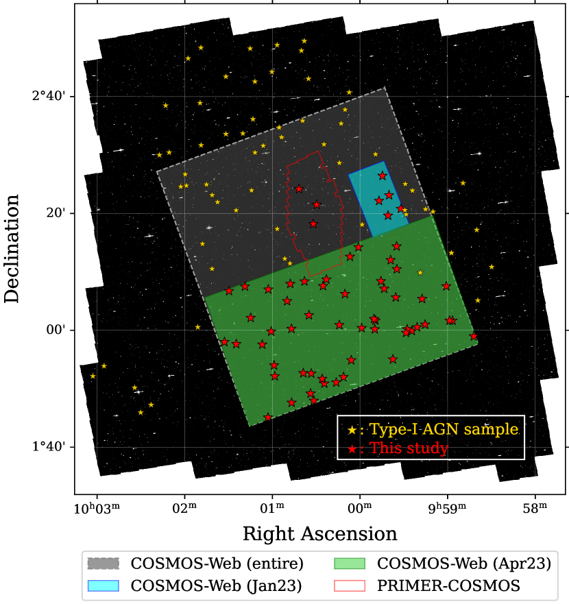
Figure 1: Location of the sample compared to the footprints of COSMOS-Web and PRIMER-COSMOS. The background is the mosaic image of HST/ACS F814W (Koekemoer et al., 2007) for the COSMOS field. Red and yellow stars show the position of each target AGN in the final sample and parent catalog, respectively. The region enclosed by the solid red line shows the PRIMER-COSMOS field, and blue and green shaded regions correspond to the observed field of COSMOS-Web (Jan23) and COSMOS-Web (Apr23), respectively. The gray region shows the region scheduled to be observed in the COSMOS-Web in December 2023 and January 2024, increasing the sample size to $\sim 100$.

COSMOS-Web (PI: Jeyhan Kartaltepe and Caitlin Casey, GO1727, see Casey et al., 2023, for the overview) is a 270-hour treasury survey program in JWST Cycle 1, covering 0.54 ${\rm deg}^{2}$ with NIRCam (Rieke et al., 2023) in four filters (F115W, F150W, F277W, F444W) and 0.19 ${\rm deg}^{2}$ with MIRI (Bouchet et al., 2015) using F770W. The COSMOS-Web field was split into three areas for observations. In this paper, we use the January 2023 data covering $\sim 0.022~{}{\rm deg^{2}}$ with six visits and April 2023 data covering $\sim 0.28~{}{\rm deg^{2}}$ with 77 visits. Due to the large field, the April 2023 data is separated into ten mosaic images. The January and April 2023 data together account for $\sim 56\%$ of the total NIRCam coverage, and the remainder of the observations are scheduled in December 2023/January 2024.

The data are reduced with the JWST Calibration Pipeline (Bushouse et al., 2023) version 1.8.3/1.10.0 and the calibration Reference Data System version 1017/1075 for January/April 2023 data, respectively. The $5\sigma$ depth in an aperture with a radius of 0$\farcs$15 has a wide range from 26.7 to 27.5 mag in F115W and 27.5 to 28.2 mag in F444W, depending on the number of integrations (also see Section 2.1 of Casey et al., 2023). The mosaic images have a resolution of 0$\farcs$030/pixel. Details of the image reduction process will be described in Franco et al.,(in preparation). In addition to NIRCam four-band data, we use HST/ACS F814W data (Koekemoer et al., 2007). In this study, we do not use MIRI data because it is challenging to apply the 2D decomposition method (Section. 3.2) to MIRI data due to its lower spatial resolution and larger PSF.

2.2 PRIMER

Public Release IMaging for Extragalactic Research (PRIMER, PI: James Dunlop, GO1837) is a 195-hour treasury program of JWST Cycle 1, targeting two equatorial HST CANDELS Legacy Fields: COSMOS and UDS. PRIMER-COSMOS covers 144 ${\rm arcmin}^{2}$ with eight NIRCam (Rieke et al., 2023) filters (F090W, F115W, F150W, F200W, F277W, F356W, F410M, F444W) and 112 ${\rm arcmin}^{2}$ with two MIRI (Bouchet et al., 2015) filters (F770W and F1800W) in the COSMOS field. The processed COSMOS-PRIMER data consists of one mosaic image. In this analysis, we use NIRCam eight-band data and HST/ACS F814W data. The PRIMER-COSMOS data are reduced with the JWST Calibration Pipeline (Bushouse et al., 2023) version 1.8.3 and the calibration Reference Data System version 1017. The $5\sigma$ depth in an aperture with a radius of 0$\farcs$15 has a wide range from 27.9 to 28.3 mag in F090W and 28.4 to 28.9 mag in F444W, depending on the number of integrations, $\sim$1 mag deeper than the COSMOS-Web data. The mosaic images have a resolution of 0$\farcs$030/pixel.

2.3 Broad-line AGN sample

To evaluate the relation between $M_{*}$ and $M_{\rm BH}$, we use the type-I AGN sample with $M_{\rm BH}$ estimates available in Schulze et al. (2015, 2018). Schulze et al. (2015) presents the redshift evolution of AGN population based on spectroscopically observed type-I AGNs from zCOSMOS (Lilly et al., 2007, 2009), VVDS (Le Fèvre et al., 2005, 2013; Garilli et al., 2008), and SDSS (Schneider et al., 2010; Shen & Kelly, 2012). Schulze et al. (2018) provides the properties of X-ray selected and spectroscopically-confirmed type-I AGNs in the FMOS-COSMOS survey (Kashino et al., 2013; Silverman et al., 2015). Here, we select the targets in Schulze et al. (2015) and Schulze et al. (2018) that are also detected by Chandra (Chandra-COSMOS Survey; Elvis et al., 2009; Civano et al., 2012) or XMM-Newton (XMM-COSMOS; Cappelluti et al., 2009; Brusa et al., 2010). The 2-10 keV flux sensitivity is $7.3\times 10^{-16}~{}{\rm erg~{}cm^{-2}~{}s^{-1}}$ for Chandra and $3\times 10^{-15}~{}{\rm erg~{}cm^{-2}~{}s^{-1}}$ for XMM-Newton.

We have $M_{\rm BH}$ estimates from spectra acquired by the FMOS-COSMOS and zCOSMOS surveys with some AGNs having measurements from both. Considering the quality of the spectroscopy, the error on $M_{\rm BH}$ estimation, and the fact that ${\rm H}\beta$ line is used for calibrating virial mass estimators, we use the $M_{\rm BH}$ from ${\rm H}\beta$ (FMOS-COSMOS), ${\rm H}\alpha$ (FMOS-COSMOS), and Mgii (zCOSMOS-Bright, Deep) in order of preference; e.g., FMOS ${\rm H}\beta$ is used for an object with both FMOS ${\rm H}\beta$ and zCOSMOS Mgii estimation. As shown in Figure 10 of Schulze et al. (2018), there is a very good agreement between the FMOS H$\alpha$- and H$\beta$-based $M_{\rm BH}$ compared to those using MgII. We note that 39 targets in our sample were also observed spectroscopically in SDSS; we do not use these SDSS Mgii-based $M_{\rm BH}$ measurements given the benefits of the FMOS and deeper zCOSMOS spectroscopy. The number and redshift range of each measurement are summarized in Table 1.

Table 1: Sample size for each single-epoch $M_{\rm BH}$ estimation

Survey	line	CW	PR	$z$ range
FMOS-COSMOS	${\rm H}\alpha$	25	3	0.69–1.7
	${\rm H}\beta$	14	0	1.2–2.5
zCOSMOS-bright	Mg ii	18	0	1.1–2.0
zCOSMOS-deep	Mg ii	1	0	0.96
Total		58	3	0.69–2.5

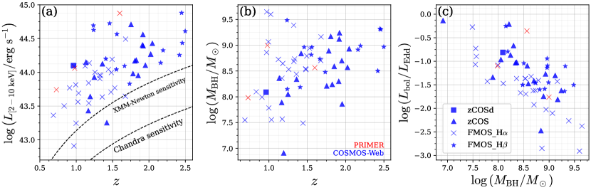
Figure 2: Characteristics of the type-I AGN sample with JWST imaging from COSMOS-Web and PRIMER: (a) Distribution of 2–10 keV X-ray luminosity $L_{\rm[2-10~{}keV]}$ as a function of $z$. Black dashed lines indicate the $F_{\rm[2-10~{}keV]}$ sensitivity in the sample, (b) Black hole mass $M_{\rm BH}$ as a function of $z$, and (c) relation between the Eddington ratio $L_{\rm bol}/L_{\rm edd}$ and $M_{\rm BH}$. The color and shape of the points indicate the JWST survey field and the source of $M_{\rm BH}$ estimation, respectively, as shown.

For ${\rm H}\beta$, Schulze et al. (2018) used the virial mass estimation relation by Vestergaard & Peterson (2006),

$$\small M_{\rm BH}\left({\rm H}\beta\right)=10^{6.91}\left(\frac{L_{5100}}{10^{44}~{}{\rm erg~{}s^{-1}}}\right)^{0.5}\left(\frac{{\rm FWHM_{\rm H\beta}}}{1000~{}{\rm km~{}s^{-1}}}\right)^{2}M_{\odot},$$ (1)

where $L_{5100}$ is continuum luminosity at 5100 Å and ${\rm FWHM_{\rm H\beta}}$ is the full-width at half-maximum (FWHM) of ${\rm H\beta}$ broad line. Then, the ${\rm H}\alpha$-based masses are calculated as given in Schulze et al. (2017, 2018),

$$\small M_{\rm BH}\left({\rm H}\alpha\right)=10^{6.71}\left(\frac{L_{{\rm H}\alpha}}{10^{42}~{}{\rm erg~{}s^{-1}}}\right)^{0.48}\left(\frac{{\rm FWHM_{\rm H\alpha}}}{1000~{}{\rm km~{}s^{-1}}}\right)^{2.12}M_{\odot},$$ (2)

$L_{{\rm H}\alpha}$ is the ${\rm H\alpha}$ luminosity and ${\rm FWHM_{\rm H\alpha}}$ is the FWHM of the broad ${\rm H\alpha}$ emission line. For Mgii-based $M_{\rm BH}$ estimation (zCOSMOS-bright Mgii, and zCOSMOS-deep Mgii), the calibration by Shen et al. (2011) is used,

$$\small M_{\rm BH}\left({\rm Mg{\sc II}}\right)=10^{6.74}\left(\frac{L_{3000}}{10^{44}~{}{\rm erg~{}s^{-1}}}\right)^{0.62}\left(\frac{{\rm FWHM_{Mg{\sc II}}}}{1000~{}{\rm km~{}s^{-1}}}\right)^{2}M_{\odot},$$ (3)

where $L_{3000}$ is continuum luminosity at rest-frame 3000 Å and ${\rm FWHM_{Mg{\sc II}}}$ is FWHM of Mgii broad emission line. These single-epoch virial mass estimations have an uncertainty due to possible variability and uncertainties in the modeling of broad-line regions (c.f., Shen, 2013). In this paper, we use the $M_{\rm BH}$ uncertainties that also consider uncertainties from the single-epoch virial mass estimation, typically $\sim 0.4~{}{\rm dex}$. We also consider this uncertainty in generating mock data (Section 3.6).

From the parent catalog, we select broad-line AGNs that reside in the COSMOS-Web and PRIMER fields. The final sample size has 61 AGNs with mass estimation summarized in Table 1. Figure 1 shows the spatial location of the AGN sample within the COSMOS-Web footprint. We use five broadband images from HST/ACS (F814W) and JWST/NIRCam (F115W, F150W, F277W, and F444W) for the sample residing in COSMOS-Web. Four more broadband (F090W, F200W, F356W) and mediumband (F410M) images are available for three galaxies in the PRIMER field.

Figure 2 shows the distribution of 2–10 keV X-ray luminosity $L_{\rm[2-10~{}keV]}$ (panel a) and $M_{\rm BH}$ (panel b) as a function of redshift, where $L_{\rm[2-10~{}keV]}$ is calculated with an X-ray spectral index $\Gamma=1.8$ (e.g., Brightman et al., 2013). Since the sample consists of X-ray-selected objects and is flux-limited, there is a tendency for higher-$z$ objects to have larger $L_{\rm[2-10~{}keV]}$ over the sensitivity limit. We can also see the trend of $M_{\rm BH}$ increasing with redshift. The sample biases likely influence this trend from the flux sensitivity and the availability of broad-line FWHM measurements from spectroscopic data. Figure 2 (c) displays the relation between the Eddington ratio $L_{\rm bol}/L_{\rm edd}$ and $M_{\rm BH}$ with Eddington ratio decreasing as $M_{\rm BH}$ increases. This trend is due to the observational flux limitation and that $L_{\rm edd}$ is proportional to $M_{\rm BH}$. While there is a correlation between $M_{\rm BH}$ and $L_{\rm bol}$, dividing $L_{\rm bol}$ by $L_{\rm edd}$ to calculate the Eddington ratio cancels out this weaker correlation between $L_{\rm bol}$ and $M_{\rm BH}$.

Figure 3 shows the F277W original images, i.e., before the decomposition analysis, of representative AGNs in our sample as examples of the images before the decomposition analysis. In some targets, we can recognize the extended components of the host galaxies far from the central PSF-like feature. However, a central AGN component, especially those with spiky diffraction features in the outer part, dominates the system and buries the host galaxy component. These dominant PSF components prevent us from obtaining host galaxy information directly and make the 2D decomposition analysis necessary.

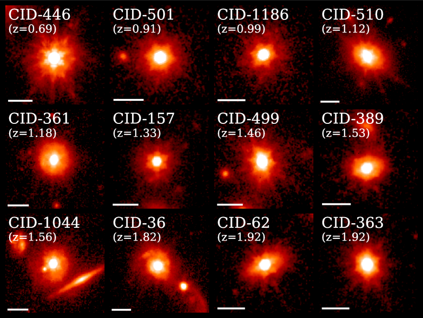
Figure 3: Original images in F277W of some targets in the order of redshift. The target IDs and the redshifts are shown in the up-left corner of each image. The white bars in the lower left part show $1^{\prime\prime}$. Depending on the host-to-total flux ratio ($H/T$) that varies in the sample, a central AGN component dominates an entire system, burying a host galactic component.

3 Method

To extract host galaxy components from the original AGN + host galaxy NIRCam images, we apply a 2D image analysis tool galight (Ding et al., 2020). With galight, we perform forward modeling of each image as a superposition of a PSF component and PSF-convolved Sérsic components corresponding to the light from an AGN and its host galaxy, respectively. We then obtain images of the host galaxy, free of the AGN, by subtracting the fitted PSF component from the original image.

3.1 Comparative analysis of model PSF construction

Considering that the AGN can account for up to $\sim 95\%$ of the total flux (e.g., Ding et al., 2020, 2022a), the results significantly depend on the accuracy of reconstructing the PSF. There are different strategies to reconstruct PSF images based on either using theoretical PSFs (e.g., Suess et al., 2022) or stellar images (e.g., Nardiello et al., 2022; Ding et al., 2022a, 2023; Zhuang & Shen, 2023; Baker et al., 2023). The former uses the theoretical PSF model such as WebbPSF (Perrin et al., 2012, 2014), and the latter uses natural stellar images as the PSF directly or modeled PSF with tools such as PSFEx (Bertin, 2011). Many previous studies concluded that the synthetic PSF simulated by WebbPSF is narrower than the PSFs reconstructed with the natural stars (Ono et al., 2022; Ding et al., 2022a; Onoue et al., 2023). Note that Ito et al. (2023) used the intermediate method between the former and the latter; they used theoretical PSFs with WebbPSF and smoothed it by comparing the surface brightness profile of natural stellar images. In this paper, we reconstruct the PSF using three methods based on natural star images for each region and filter. Then, we compare the results with the different PSF reconstruction methods and discuss the host galaxy characteristics with the method dependence.

3.1.1 $\chi^{2}_{\nu}$-based methods

First, we follow the strategy of Ding et al. (2020, 2022a). They first construct an empirical PSF library for which each PSF is represented by the image of a single star. Then, the 2D decomposition analysis is run with all single PSFs in the library, separately. Then, they sort the results in the order of reduced chi-square $\chi^{2}_{\nu}$ and stack the PSFs with the top 3, 5, and 8 $\chi^{2}_{\nu}$ values. Using the single PSFs and the stacked PSFs, they select the PSF with the smallest $\chi^{2}_{\nu}$ as the final PSF. This method is based on the $\chi^{2}_{\nu}$; i.e., they assumed that the lower $\chi^{2}_{\nu}$ is indicative of a better (the closer to the more accurate) PSF.

Following their strategy, we apply the find_PSF function in galight to list PSF candidates, then select PSF candidates manually for each mosaic image and filter. In this manual selection process, only obvious PSF candidates with the PSF-like complex hexagonal and spiky diffraction features and without a galaxy-like broad component are selected. We cropped the images of the selected PSF candidates for the short-wavelength-channel filters (F090W, F115W, F150W, and F200W) and long-wavelength-channel filters (F277W, F356W, F410M, and F444W) as squares with 150 and 240 pixels per side, corresponding to 4$\farcs$5 and 7$\farcs$2, respectively. After removing neighbor objects using clean_PSF function in galight, the PSF libraries contain $\sim 30-50$ PSF candidates depending on the filter and region. Then, we fit each AGN target with a superposition of a PSF-convolved Sérsic profile and each single PSF candidate in the PSF library. With the fitting results of each single-PSF, we select PSFs with the top-5 $\chi^{2}_{\nu}$ and top-75% $\chi^{2}_{\nu}$ and stack them to generate an averaged PSF image. These top-5 stacked and top-75% stacked PSFs are finally used to estimate the parameters in this method. Note that each target has its own top-5 and top-75% PSFs generated from single PSFs with the lowest $\chi_{\nu}^{2}$ selected for each target.

3.1.2 Modeling method

Zhuang & Shen (2023) compare JWST/NIRCam PSFs modeled with different methods (Swarm, photutils, and PSFEx), and concluded PSFEx reconstructed PSFs provide the best performance. From the 2D decomposition of simulated broad-line AGNs, Zhuang & Shen (2023) also suggested that smaller $\chi^{2}_{\nu}$ values do not necessarily provide a means to distinguish which PSFs are more likely to characterize the AGN with higher accuracy. Following the conclusion by Zhuang & Shen (2023), we use PSFEx and compare the results with $\chi^{2}_{\nu}$-based selected PSFs (Section 3.1.1).

PSFEx constructs an empirical PSF model based on the output catalog of SExtractor (Bertin & Arnouts, 1996). We first run SExtractor for source detection, and then run PSFEx for modeling the PSF for each mosaic image and filter. PSFEx can also reconstruct local PSFs as a function of positions on the detector. We do not use local PSFs because Zhuang & Shen (2023) also concluded that a universal or global PSF usually shows “satisfactory” fitting results, and the sample region (COSMOS-Web and PRIMER-COSMOS) have a much smaller number of stars than the south continuous viewing zone, which Zhuang & Shen (2023) tested local PSF reconstruction.

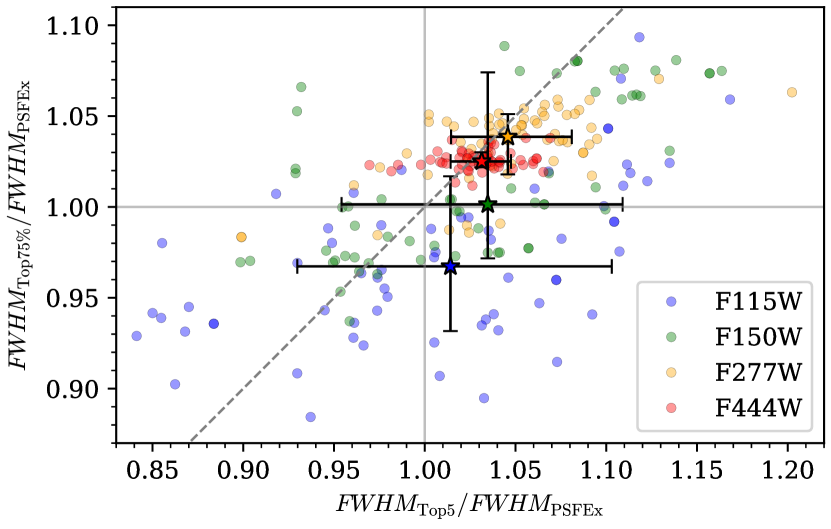
Figure 4: Comparison of FWHM (semi-major axis) for PSFs from different PSF reconstruction methods for all individual AGNs. The x-axis represents the ratio of the FWHMs for the top-5 PSFs to those for the PSFEx PSFs, and the y-axis represents the ratio of the FWHMs for the top-75% PSFs to those for the PSFEx PSFs. Blue, green, orange, and red colors indicate the different filters: F115W, F150W, F277W, and F444W. Median values and $1\sigma$ confidence range are denoted by star symbols and error bars. The gray dashed line indicates $y=x$, i.e., the same FWHMs for the top-5 and top-75% PSFs. Notably, F277W and F444W exhibit a FWHM bias among different PSF reconstruction methods.

3.1.3 Comparing the final PSFs

Now, we have three final PSFs for comparison; the top-5 $\chi^{2}_{\nu}$ stacked PSF, the top-75% $\chi^{2}_{\nu}$ stacked PSF, and the PSFEx PSF (Sections 3.1.1 and 3.1.2). To compare PSFs, we perform, a 2D Gaussian fitting for each PSF image and measure the FWHMs along the semi-major axis. Figure 4 compares the FWHMs of PSFs obtained with each method, target, and filter. The x and y-axis of Figure 4 show the ratio $FWHM_{\rm Top-5}/FWHM_{\rm PSFEx}$ and $FWHM_{\rm Top-75\%}/FWHM_{\rm PSFEx}$, where $FWHM$ is the value along the semi major axis.

Firstly, regardless of the filters, we can see that the distribution extends further in the x-axis direction than the y-axis. This can be attributed to greater variation in the FWHMs for the top-5 stacked PSFs. We use the same PSFEx PSF for each target in the same field, and the top-75% stacking in the same field uses mostly the same single PSFs in the field. In contrast, top-5 stacking employs only the best-fit single PSFs with the lowest $\chi^{2}_{\nu}$. As a result, the FWHM variation for each galaxy is largest for the top-5 PSF followed by the top-75% PSF and PSFEx PSF, and $FWHM_{\rm Top-5}/FWHM_{\rm PSFEx}$ have a larger scatter than $FWHM_{\rm Top-75\%}/FWHM_{\rm PSFEx}$.

Secondly, we focus on the FWHM bias between the methods for each filter. As suggested by Zhuang & Shen (2023), for short-wavelength filters (F115W and F150W), there is a significant scatter in the FWHM ratio. On the other hand, for long-wavelength filters (F277W and F444W), the scatter is smaller than the short-wavelength side. These results imply that, in the long-wavelength filters, PSFEx PSFs are sharper than the top-5 and Top-75% PSFs. The impact of these trends on the 2D decomposition analysis is discussed in Section 4.2.

Note that these trends can depend on the visual inspection performed when constructing the PSF library (Section 3.1.1) and the settings used for Sextractor and PSFEx (Section 3.1.2). For example, visual inspection can be biased by the hexagonal diffraction features of the JWST PSF, an appropriate FWHM range, and the absence of extended structures originating from host galaxies. If this selection process is strongly biased by the hexagonal features, it might lead to a selective choice of brighter PSFs. As a result, the parameter distributions presented here may not necessarily match the distribution of the actual PSF. Nonetheless, even different PSF reconstruction methods can result in different FWHMs. Therefore, when performing a 2D decomposition analysis with only one PSF reconstruction method and not considering the possibilities of other PSFs, 2D decomposition results can be biased by a specific PSF. Because determining the PSF shape perfectly is challenging, it is also important to discuss uncertainties by considering the results obtained with possible different PSFs. We discuss how different PSF reconstruction methods affect the results of the 2D decomposition and the final $M_{*}$ estimation in Section 4.2, and we perform a detailed comparison of the obtained final PSFs in appendix B.

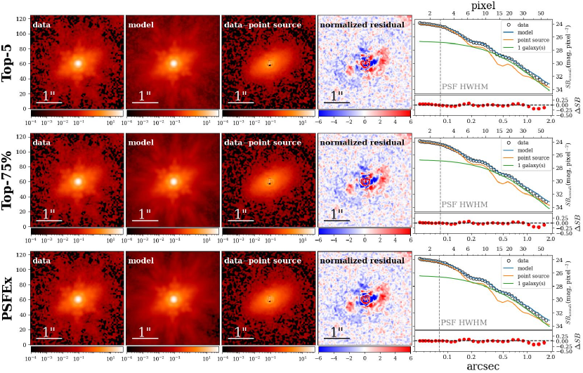
Figure 5: Example fits for CID-62 ($z\sim 1.92$) using F444W. Each row shows results for a different PSF (top-5 stacked, top-75% stacked, and PSFEx, from top to bottom). In each row, the images are as follows: original, model, data – model point source (host galaxy only), and normalized residuals, from left to right. The right panel shows the 1D surface brightness profile where dashed lines indicate half-width at half-maximum (HWHM) of each PSF. In the data-point source image, we reveal a disk-like host galaxy which is buried under the PSF before subtraction, regardless of the PSF reconstruction method.

3.2 Decomposition

Using galight, we fit the AGN + host galaxy images with the composite model of a PSF component and a single Sérsic profile (Sérsic, 1968) convolved by a PSF. Note that we do not assume the same morphology in every wavelength, and the fitting is performed in each filter independently. In the case there are nearby galaxies that can affect the fitting, those galaxies are also modeled as Sérsic components and fitted simultaneously. Our Sérsic model has seven free parameters: amplitude, Sérsic index $n$, effective radius $r_{e}$, coordinates of the center $x_{c},y_{c}$, and ellipticity parameters $e_{1},e_{2}$. The PSF model corresponding to the AGN component has three free parameters: amplitude and coordinates of the center $x_{c},y_{c}$. Thus, the number of free parameters for PSF + single Sérsic component is ten in total. Note that the actual number of free parameters in the fitting changes depending on the number of nearby objects also fitted with a Sérsic profile.

To avoid unphysical results, the range of $n$ and $r_{e}$ is constrained to $\left[0.3,9\right]$ and $\left[0\farcs 06,2\farcs 0\right]$, respectively. Note that some galaxies show clear substructures that do not suit a Sérsic profile, such as bars and spiral arms. Thus, using a Sérsic profile is a first-order approximation to model the global component of AGN host galaxies.

In the fitting process, first, we cut the image into square regions centered on the target and with a radius seven times the standard deviation along the semimajor axis of the 2D Gaussian fitting with photutils (Bradley et al., 2023). Then, the above model is optimized with Particle Swarm Optimizer (PSO; Kennedy & Eberhart, 1995). galight also supports Markov Chain Monte Carlo (MCMC) to estimate the posterior parameter distributions. As Ding et al. (2023) suggested, we also confirm that the uncertainty estimated with MCMC is much smaller than the uncertainties from different PSFs. Thus, we do not use MCMC in the decomposition analysis, and we estimate the uncertainty from the results with different single PSFs (Section 3.4). We set the supersampling factor relative to pixel resolution to 3, which controls interpolation within a pixel to perform a subpixel shift of the PSF (c.f., Ding et al., 2023).

As described above, for the PSF library constructed with galight, we fit with every single PSF in the library and sort them in order of $\chi^{2}_{\nu}$. Then we fit with the three final PSFs; top-5 $\chi^{2}_{\nu}$ stacked, top 75% $\chi^{2}_{\nu}$ stacked, and PSFEx. Figure 5 compares the fitting results with the final PSFs for the example galaxy CID-62 in the F444W. We can find that 2D decomposition makes it possible to detect the host galaxy initially buried under the PSF component with all three model PSFs.

For targets that have $n>8.5$ in any band other than F277W, we rerun the fit while fixing $n$ to the value found for the F277W band. This filter has the lowest number of values hitting the upper limit on $n$, falls above the rest-frame 4000 Å break, and is somewhat central to JWST wavelength coverage. This pertains to 10, 11, and 7 sources detected in F115W, F150W, and F444W, respectively. From the mock test, we confirm that galight can return $n\sim 9$ even if the actual value is much smaller (Appendix C). This is likely due to fitting where some of the AGN emission is attributed to a central stellar concentration of the host thus overestimating the host galaxy flux as well.

3.3 Detection of host galaxy

Figure 5 shows an example where the host galaxy is clearly detected. However, for some galaxies, the strong PSF component dominates the total flux maybe due to not only a low host-to-total flux ratio $H/T$ but also compact morphology, making it challenging to distinguish the host signal from their PSF component. To gauge, in a quantitative manner, which AGNs have accurate host galaxy information, we exclude cases where the host galaxy is undetectable, following three strategies below.

(1) Bayesian Information Criteria: In addition to the PSF + Sérsic model (PS+SE model) described above, we also fit with a model containing only a PSF component (PS model). Then we calculate Bayesian Information Criteria (BIC; Schwarz, 1978) for the two models, PS+SE and PS model, as,

$${\rm BIC}=-\frac{1}{2}\chi^{2}+k\ln\left(n\right),$$ (4)

where $k$ is the number of free parameters, and $n$ is the number of data points. We regard that the PS+SE model provides a better description of the data than the PS model when ${\rm BIC_{PS+SE}}$ is much smaller than ${\rm BIC_{PS}}$, as

$${\rm BIC_{PS+SE}}<{\rm BIC_{PS}}-10,$$ (5)

We decide the threshold value of the BIC difference of 10 based on Kass & Raftery (1995).

(2) $S/N$ of the host galaxy: To estimate the significance of the detection of the host galaxy, we calculate the $S/N$ of the host galaxy as done in Ding et al. (2023). We construct an error map of the PSF-subtracted images considering two sources of error: noise from the observed images and the uncertainty propagated from different PSF reconstructions. Due to the intrinsic variations of the PSF image even in the same FoV (Zhuang & Shen, 2023; Yue et al., 2023) and errors in the observed image used in PSF reconstruction, the reconstructed PSFs contain uncertainties. Thus, considering the uncertainty from PSF reconstruction is indispensable to calculate the $S/N$ of detected host galaxies. For the PSF uncertainty, we use the pixel-by-pixel standard deviation of the fitted PSF components when fitting the PS+SE model with each single PSF in the PSF library. Then, we calculate the final noise map as a composite of the observed noise map and the PSF uncertainty map. With the final noise map, we calculate the signal-to-noise ratio of host galaxy $S/N_{\rm host}$ within a radius of 2$r_{e}$. Then, we define the detection as cases with high $S/N_{\rm host}$, as

$$S/N_{\rm host}>5.$$ (6)

(3) Manual inspection and removal: We find that some objects have invalid central values in their F444W image and shallower surface brightness profiles than any PSFs. The fitting of these galaxies fails even with applying a mask in the central region. We find two cases (CID-50 and CID-208) with such features and label them as non-detections.

As a more challenging case, CID-166 passes the conditions (1) and (2) but clearly shows PSF-like features not completely removed. Since CID-166 does not show a host-like component in the PSF-subtracted images in any filter, the host galaxy seems to be an extremely low-$H/T$ or compact object (see AppendixC for the limitation of detecting hosts). Therefore, we manually exclude CID-166 in the following discussion.

We also find some obvious false detections in F814W, where the image shows a dominant PSF feature and no extended host-like feature, and galight fit the PSF-like features as a host galaxy with $H/T\sim 1$. We confirm that the decomposition of the JWST images clearly detects a host-like extended feature. Thus, in addition to the above strategies, we recognize 16 obvious false detections in F814W as non-detection cases.

With the above three strategies, we confidently report the detection of an AGN host galaxy for those that fulfill both the conditions (5) and (6) for each of the final PSFs; i.e., we determine whether the host is detected or not for each top-5, top-75%, and PSFEx PSF, separately. Also note that this decision is made for each sample and each filter, i.e., a galaxy detected in one filter may not be detected in another filter. The number of objects which is detected over one (two) filters of NIRCam is 60 (55), occupying $\sim 98\ (90)\%$ out of the entire $N=61$ sample with the top-5 PSF (see Appendix A for the number of detection in each filter).

3.4 Photometry of host galaxies

We calculate the Sérsic flux of the host galaxies considering Galactic dust extinction (Schlegel et al., 1998) for the detected cases. On the uncertainty of photometry, we set a larger error of 0.2 mag, which represents likely systematic uncertainties (e.g., Ding et al., 2022a; Zhuang & Shen, 2023; Zhuang et al., 2023) and errors discussed in Section 3.3, which considers both observational errors and PSF uncertainty in a radius of 2$r_{e}$. We use the $3\sigma$ value for the undetected filters as the upper limit.

Here, we also fit with a model containing only a Sérsic component (SE model). For targets with ${\rm BIC_{PS+SE}}>{\rm BIC_{SE}}-10$, the SE model is better or flexible enough to describe the data than the PS+SE model, and we use the Sérsic photometry calculated with the SE model instead of the PS+SE model. Such cases are observed only in F444W and are very limited (two or three objects depending on the PSF).

3.5 SED fitting

We fit the photometry of the host galaxies with CIGALE (v2022.1, Boquien et al. 2019; Yang et al. 2022) SED fitting library. For a stellar population, we use the single stellar population model by Bruzual & Charlot (2003) (bc03 module) and the Chabrier initial mass function (IMF; Chabrier, 2003) with the $M_{*}$ cutoff of $0.1M_{\odot}$ and $100M_{\odot}$ (Bruzual & Charlot, 2003). We assume a delayed-$\tau$ model for a star-formation history (SFH), where SFR at each look-back time $t$ is modeled as

$$SFR\left(t\right)\propto\begin{cases}\left(t-t_{\rm age}\right)\exp\left(-\frac{t-t_{\rm age}}{\tau}\right)&\left(t>t_{\rm age}\right),\\ 0&\left(t<t_{\rm age}\right),\end{cases}$$ (7)

where $t_{\rm age}$ and $\tau$ indicate the starting time of star-formation activity and the declining timescale of SFR. We also consider a nebular emission with nebular module and a dust attenuation with dustatt_modified_starburst module that assumes the modified Calzetti et al. (2000) law. We set $E\left(B-V\right)$, $M_{*}$, $t_{\rm age}$, and $\tau$ as free parameters; their grid values are decided basically following Zhuang et al. (2023) CIGALE run and summarized in Table 2. To avoid unphysical solutions, we set the upper limit of $t_{\rm age}$ to $0.95t_{H}$, where $t_{H}$ indicates the cosmic age at each redshift. Otherwise, stellar metallicity and the ionization parameter $U$ are fixed at Solar metallicity and $\log U=-2$.

Table 2: Major parameter settings in SED fitting

parameter	description	values (CIGALE)	prior (Prospector)
$\log\left(M_{*}/M_{\odot}\right)$	total stellar mass	Scaled with the data	Uniform: min=9, max=13
$\log\left(Z_{*}/Z_{\odot}\right)$	stellar metallicity	Fixed at 0	Fixed at 0
$\log U$	ionization parameter	Fixed at -2	Fixed at -2
$E\left(B-V\right)/{\rm mag}$	Color excess for the nebular lines	0, 0.001, 0.005, 0.01, 0.03, 0.05, 0.1, 0.2, 0.3, 0.4, 0.5, 0.6, 0.7
$\hat{\tau}_{\rm dust,2}$	optical depth of the diffuse dust attenuation		Uniform: min=0, max=3
$\tau/{\rm Gyr}$	timescale of delayed-$\tau$ SFH	0.01, 0.05, 0.1, 0.25, 0.5, 0.75, 1.0, 1.25, 1.5, 2.0, 2.5, 3.0, 3.5, 4.0, 4.5, 5.0, 6.0, 7.0, 8.0, 9.0, 10, 12, 14, 16, 18, 20	Uniform in $\log\left(\tau/{\rm Gyr}\right)$: min=-2, max=1.5
$t_{\rm age}$/Gyr	starting time of delayed-$\tau$ SFH	equally sampled in [1 Gyr, 1.95$t_{H}$] with the separation of 0.1 Gyr	Uniform: min=1, max=0.95$t_{H}$

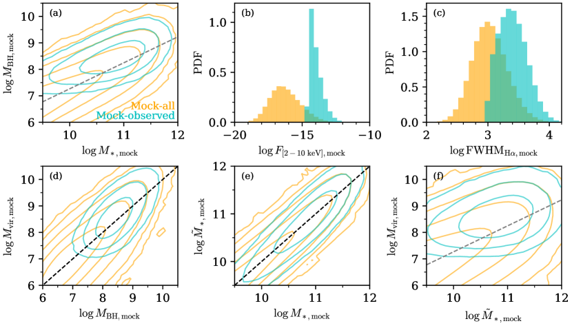
Figure 6: Procedure for generating mock galaxies at $z\sim 1.5$ with an example parameter set of $\alpha=\alpha_{\rm local}$, $\beta=\beta_{\rm local}$, $\gamma=0$, $\sigma_{\mu}=0.4$. Orange and blue contours show the distribution of the entire sample ($1\sigma-5\sigma$) and that above the detection limit of the observed sample ($1\sigma-3\sigma$, see Sections 5.1 for the definition of the detection). The individual panels are as follows: (a) true black hole mass $M_{\rm BH,mock}$ - true stellar mass $M_{\rm BH,mock}$, before adding observational uncertainties, (b) $2-10~{}{\rm keV}$ flux ($F_{[2-10~{}{\rm keV}]),{\rm mock}}$), (c) ${\rm H\alpha}$ FWHM (${\rm FWHM}_{\rm H\alpha,mock}$), (d) pseudo-observed virial mass $M_{\rm vir,mock}$ - true black hole mass $M_{\rm BH,mock}$ where $M_{\rm vir,mock}$ is the mock black hole mass after considering the observational bias. (e) pseudo-observed stellar mass $\tilde{M}_{\rm*,mock}$ - stellar mass $M_{\rm*,mock}$ where $\tilde{M}_{\rm*,mock}$ is the stellar mass after considering the observational bias, and (f) pseudo-observed virial mass $M_{\rm vir,mock}$ - pseudo-observed stellar mass $\tilde{M}_{\rm*,mock}$. The latter is to be compared with the observed $M_{\rm BH}-M_{*}$ plane shown in the left panel of Figure 12. Black dashed lines in panels (a) and (f) indicate $M_{\rm BH}-M_{*}$ local relation obtained from the fitting of the local galaxies (Häring & Rix, 2004; Bennert et al., 2011b, , see Section 5), and gray dashed lines in panels (d) and (e) indicate $y=x$ line.

We also apply the Bayesian-based spectral energy density (SED) fitting code, Prospector (Leja et al., 2017; Johnson et al., 2021), to see the $M_{*}$ estimation uncertainty with different SED fitting codes. Prospector is based on the Flexible Stellar Population Synthesis (FSPS, Conroy et al. (2009); Conroy & Gunn (2010)) to generate model SEDs of galaxies. For the comparison, we use almost the same settings with the CIGALE described above: the Chabrier IMF, a delayed-$\tau$ SFH model, Solar metallicity, Calzetti et al. (2000) dust attenuation law, and nebular emission with $\log U=-2$. Prospector can fit with the non-parametric SFH, which separates galaxy formation history into several age bins and assumes a constant SFR in each bin (e.g., Leja et al., 2019). Lower et al. (2020) input cosmological hydrodynamic simulation data into Prospector and concluded that non-parametric SFH tends to reconstruct $M_{*}$ more accurately than parametric SFHs. Lower et al. (2020) also suggested that parametric SFH tends to underestimate $M_{*}$. However, in this study, the available photometries are limited in the number and wavelength range (only five/nine bands in the near-infrared wavelength range for the COSMOS-Web/PRIMER-COSMOS field). Furthermore, the photometry derived in Section 3.4 contain uncertainties from the 2D decomposition analysis. Therefore, we choose to use the parametric SFH (delayed-$\tau$ model) instead of the non-parametric assessment. The parameter prior settings in the MCMC run are summarized in Table 2. We compare the results with CIGALE and Prospector in Section 4.4.

3.6 Generating mock data to consider selection effects

As mentioned, our sample is X-ray-flux limited (Section 2.3), raising the possibility of bias toward larger $M_{\rm BH}$ or higher Eddington ratio (Lauer et al., 2007; Schulze & Wisotzki, 2011, 2014). Due to this selection effect, a direct comparison of the observational results with the local relation is not appropriate. Thus, in this study, we generate a mock AGN-galaxy catalog based on the procedure in Li et al. (2021) and apply the mock observation (adding selection biases and observational effects) to discuss the intrinsic evolution of the mass relation. The procedure for generating the mock catalogs is described below.

First, we generate the mock redshift $z_{\rm mock}$ and mock true stellar mass $M_{*,{\rm mock}}$ based on the COSMOS2020 stellar mass function (SMF) by Weaver et al. (2023). Next, we use the $M_{*,{\rm mock}}$ to generate the mock true BH mass $M_{\rm BH,mock}$ for the mock sample. Here, we assumed the local relation as

$$\log\left(\frac{M_{\rm BH}}{M_{\odot}}\right)=\alpha\log\left(\frac{M_{*}}{M_{\odot}}\right)+\beta,$$ (8)

where $\alpha$ and $\beta$ indicate the slope and the intercept of the local $M_{\rm BH}-M_{*}$ plane. Then, assuming a normal distribution, we calculate $M_{\rm BH,mock}$ as,

$$\log M_{\rm BH,mock}=\mathcal{N}\left(\alpha\log\left(\frac{M_{*}}{M_{\odot}}\right)+\beta+\gamma\log\left(1+z\right),\sigma_{\mu}^{2}\right).$$ (9)

Here, the parameter $\gamma$ indicates the strength of redshift evolution of the mass relation, and $\sigma_{\mu}$ is the intrinsic scatter of the mass relation. Figure 6 (a) shows $M_{\rm BH,mock}-M_{*,{\rm mock}}$ distribution with the example parameter set of $\gamma=0,\sigma_{\mu}=0.4$.

Then, based on $z_{\rm mock}$ and $M_{\rm BH,mock}$, we assign mock Eddington ratio $\lambda_{\rm Edd,mock}$ by sampling the Eddington ratio distribution function by Schulze et al. (2015). Using the $\lambda_{\rm Edd,mock}$ and $M_{\rm BH,mock}$, we calculate the bolometric luminosity $L_{\rm bol,mock}$.

From $L_{\rm bol,mock}$, we obtain $L_{[2-10~{}{\rm keV}],{\rm mock}}$ using the bolometric correction by Duras et al. (2020). With the calculated $L_{[2-10~{}{\rm keV}],{\rm mock}}$, mock X-ray flux $F_{[2-10~{}{\rm keV}],{\rm mock}}$ is determined with the assumption of $\Gamma=1.8$, the same assumption as in Section 2.3. Figure 6 (b) shows $F_{[2-10~{}{\rm keV}],{\rm mock}}$ distribution with the example parameter set of $\gamma=0,\sigma_{\mu}=0.4$.

We also generate mock virial BH mass $M_{\rm vir,mock}$ with the $L_{\rm bol,mock}$, $M_{\rm BH,mock}$, and the assumed FWHM distribution. We first calculate mock continuum and line luminosity $L_{5100,{\rm mock}}$, $L_{3000,{\rm mock}}$, and $L_{{\rm H\alpha,mock}}$. For $L_{5100,{\rm mock}}$ and $L_{3000,{\rm mock}}$, we used the bolometric correction by Netzer & Trakhtenbrot (2007) and Trakhtenbrot & Netzer (2012), respectively. For $L_{\rm H\alpha,mock}$, we use the $L_{5100,{\rm mock}}$ and scaling relation between $L_{{\rm H\alpha}}$ and $L_{5100,{\rm mock}}$ by Jun et al. (2015). These bolometric correction and scaling relations are the same as those in Schulze et al. (2018). Then, we assume that FWHM of the emission line follows the log-normal distribution with the scatter of 0.17 dex (Shen et al., 2008), and we generate the observed FWHM of ${\rm H\alpha}$, ${\rm H\beta}$, and ${\rm Mg{\sc II}}$ emission lines following Equations (1), (2), and (3). To consider the bias in single-epoch virial mass estimation, we add the bias with $\beta_{\rm bias}=0.6$ in calculating FWHM. $\beta_{\rm bias}$ represents the proportion by which $\Delta L$, the variation of luminosity from the mean luminosity $\bar{L}$, affects the variation in FWHM. Thus, the FWHM is generated by a lognormal distribution with the scatter of 0.17 dex and the mean value corresponding to the luminosity of $\bar{L}+\beta\Delta L$ (c.f. Shen, 2013; Li et al., 2021). Finally, the mock virial BH mass $M_{\rm vir,mock}$ is calculated using the mock observed FWHM and the luminosity following Equations (1), (2), and (3). Figures 6 (c) and (d) show the $FWHM_{\rm H\alpha,mock}$ histogram and $M_{\rm vir,mock}-M_{\rm BH,mock}$ distribution with the example parameter set of $\gamma=0,\sigma_{\mu}=0.4$.

Considering possible systematic uncertainties from 2D decomposition analysis, we added an error based on a normal distribution with 0.2 dex to the $M_{*,{\rm mock}}$ to consider the uncertainty of $M_{*}$ derived from observations, resulting in the mock observed stellar mass $\tilde{M}_{*,{\rm mock}}$. The resulted $\tilde{M}_{*,{\rm mock}}-M_{*,{\rm mock}}$ distribution is shown in Figure 6 (e).

Finally, we get the mock data set of the redshift $z_{\rm mock}$, observed stellar mass $\tilde{M}_{*,{\rm mock}}$, and virial BH mass $M_{\rm vir,mock}$. Figure 6 (f) shows the final mock observed mass distribution ($M_{\rm vir,mock}-\tilde{M}_{*,{\rm mock}}$) with the example parameter set of $\gamma=0$, $\sigma_{\mu}=0.4$. In Section 5, we discuss the mass relation, comparing our results with this mock catalog.

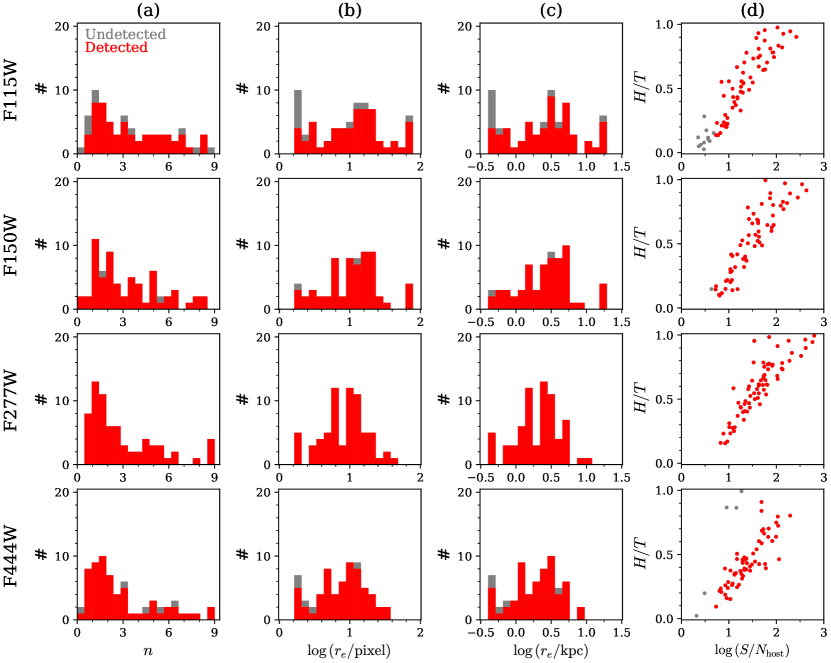
Figure 7: Summary of the decomposition results in each filter. Columns (a), (b), and (c) respectively show the distribution of the estimated $n$, $\log r_{e}$ in the unit of pixel and kpc. In column (d), the relation between $H/T$ and $S/N_{\rm host}$ is shown. In each panel, red (gray) indicates detection (non-detection) in each filter.

4 Results of AGN - host decomposition

Firstly, we examine the results obtained from the 2D decomposition.

4.1 Morphological parameters

In Figure 7 (a)–(c), we show the distribution of $n$ and $r_{e}$ (in the unit of pixel and kpc) for each filter using the top-5 stacked PSF. The distribution of $n$ has a peak in the distribution at $n\sim 1-2$, clearly seen in the F277W and F444W filters. This is similar to studies of AGN hosts at high redshift, which show hosts characterized by disk-like morphology.

In Figure 7 (d), we compare $H/T$ with $S/N_{\rm host}$. We can see a strong correlation between the reconstructed $H/T$ and $S/N_{\rm host}$. High $H/T$ means host galaxies dominate the AGN + host galaxy composite images, and we can easily detect host galaxies with high $S/N_{\rm host}$; thus, our results indicate the validity of our analyses for the majority of the sample. Estimated morphological parameters and basic information for each host galaxy are reported in Table 3. In Appendix C, we confirm that galight can reconstruct $r_{e}$ and $H/T$ correctly by running galight on mock galaxy images.

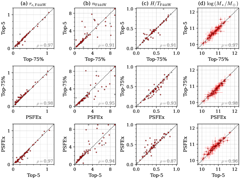
Figure 8: Comparison of the decomposition results ($r_{e}$ in the unit of arcsec, $n$, and $H/T$) based on the F444W filter using different PSFs (Columns a–c). Data points in red have satisfied our stringent criteria for host detection (Sec. 3.3). Column (d) compares $M_{*}$ estimated by the SED fitting, with colors corresponding to whether each object was detected in more than two bands. Spearman’s correlation coefficient $\rho$ for each prior is shown in the lower right corner of each panel. High correlation coefficients and the distribution around $y=x$ (black dashed line) suggest consistent results among the fitting with different PSFs.

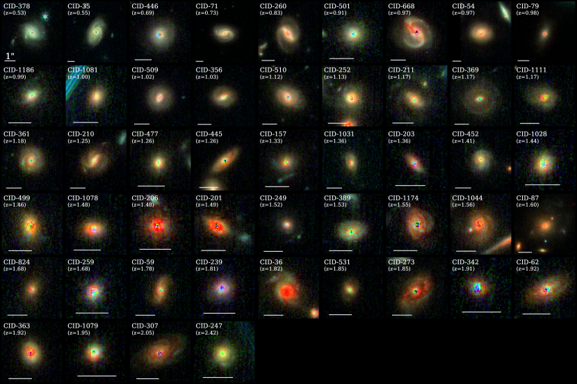
Figure 9: Three-color cutout PSF-subtracted images (the F277W, F150W, and F115W for RGB) of all host galaxies detected in all F115W, F150W, and F277W in the order of redshift. We have not performed deconvolutions based on the PSF FWHM differences between each filter, and consequently, each filter image possesses a different-sized PSF. The target IDs and the redshifts are shown in the up-left corner of each image. The white bars in the lower left part are $1^{\prime\prime}$ in length. Thanks to the high spatial resolved deep observation of JWST and the careful decomposition analysis, we can clearly identify substructures, such as bulges, spirals, bars, and dust lanes.

4.2 Impact of different PSF models

In Figure 8 (a)–(c), we compare morphological parameters, $n$, $r_{e}$, and the host-to-total flux ratio $H/T$, in F444W obtained using each final PSFs. These parameters fall mostly along the $y=x$ line, indicating a strong correlation. Thus, we can say that different PSF reconstruction methods do not significantly affect the results.

In Figure 8 (a), the size ($r_{e}$) comparison shows more consistent results than $n$, indicating that it is minimally affected by different PSFs. On the other hand, in comparing $n$ (Figure 8 (b)), regardless of the PSF, we can find a consistent estimation on the low $n$ side ($n\lesssim 3$). However, at larger $n$ ($\gtrsim 4$), the scatter increases. This tendency is likely because larger $n$ implies a compact Sérsic profile that resembles the PSF, making it challenging to distinguish from the PSF. We also find a tendency that PSFEx PSFs result in slightly larger $n$ than the top-5 or top-75% stacked PSFs. Even when considering the other filters, we find highly consistent results, with a trend of increased scatter at higher $n$.

Regarding $H/T$, we primarily see consistent results with strong correlations in Figure 8 (c). While $H/T$ estimated using the top-5 and top-75% PSFs is largely consistent with each other, the PSFEx PSFs tend to result in slightly higher $H/T$ than the other two PSFs. Zhuang & Shen (2023) suggested that using a narrower PSF than an exact PSF could overestimate the host flux and $n$. Thus, the above biases in $n$ and $H/T$ could be explained by the fact that PSFEx PSFs for F444W have a slightly narrower PSF than the other PSFs, as shown in Figure 4. A detailed comparison of the estimated $H/T$ in other filters is summarized in Appendix B.

In conclusion, the decomposition results using different PSFs are generally highly consistent with each other. A comprehensive discussion of the technical and practical differences between PSF reconstruction methods will also be provided in Section 6.3. Nonetheless, these discussions are based on the comparisons between estimated values, and here, we cannot definitively determine the true exact value. Related to this, we provide the result of mock tests using different final PSFs in Appendix C. Also, note that all final PSFs are not single stellar images but stacked or modeled PSFs based on multiple stellar images. As mentioned in Section 3.1.3, single PSFs often have a wide range of sizes and shapes. Thus, using a single stellar image without testing other stellar images can risk misinterpreting the PSF image and giving different results.

4.3 Host images

As seen in these high-quality host galaxy images, 2D decomposition analyses of JWST images open up the potential for a more detailed image-based galaxy analysis, such as studies traditionally conducted on inactive galaxies. Figure 9 shows three-color images (F277W, F150W, and F115W for RGB) of each host galaxy created by subtracting the PSF and the nearby Sersic component.

Firstly, thanks to the high spatial resolution, deep observations, and meticulous decomposition analysis, we can access the highest-quality AGN-host galaxy images up to $z\sim 2.5$, allowing us to identify substructures. Particularly, in the case of CID-273 ($z=1.85$) and CID-307 ($z=2.05$), despite their redshifts $\sim 2$, we can clearly identify blue spiral arms with an overall diffuse red broad component.

Additionally, galaxies such as CID-54 ($z=0.97$), CID-510 ($z=1.12$), CID-361 ($z=1.18$), CID-445 ($z=1.26$), and CID-452 ($z=1.41$) show more reddish colors at their centers than in the outer region, indicating the possibility of having a bulge-like structure or highly dust-obscured region. Furthermore, there are cases with extended red structures (e.g., CID-668; $z=0.97$) which may indicate the presence of dust lanes as seen in the X-ray obscured (type-II) AGNs (Silverman et al., 2023).

4.4 Estimated $M_{*}$ and the comparison of different SED fitting methods

As described in Section 3.5, we perform SED fitting of the host galaxy photometry to estimate $M_{*}$. The inferred $M_{*}$ for each host galaxy is reported in Table 3. Figure 10 shows four examples of the SED fitting results with the residuals. Generally, for the objects with $z\gtrsim 1$, the photometry or upper limit from F814W and F115W fall at a rest-frame wavelength shorter than 4000 Å break and are important in constraining stellar population parameters of host galaxies.

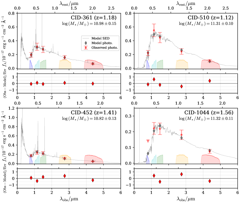
Figure 10: Representative examples of SED fits to PSF-subtracted host galaxies. Source ID and their estimated $M_{*}$ with 1$\sigma$ confidence range are shown in the top right corner of each plot. The inverted triangle indicates the $3\sigma$ upper limit due to the non-detection in each filter. The bottom colored shades show the transmission curves of F814W, F115W, F150W, F277W, and F444W from left to right. The lower plot in each panel shows the difference between the observational and best-fit model photometry scaled by the error of the data.

Table 3: Data summary of our sample.

CID	XID	$z$	R.A.	Decl.	$\log M_{\rm BH}$	line	$\log M_{*}$	$r_{e,{\rm F115W}}$	$n_{\rm F115W}$	$\log H/T_{\rm F115W}$
			[deg]	[deg]	$[M_{\odot}]$		$[M_{\odot}]$	[′′]
157	5404	1.33	149.6751	1.9828	8.73	2	$10.74\pm 0.13$	0.83	5.6	0.37
162	169	2.46	149.7359	2.0276	9.30	1	$11.47\pm 0.02$	0.06	9.0	0.12
1489	54330	1.95	149.7536	2.1256	7.86	3	$10.59\pm 0.12$	0.06	3.6	0.20
203	341	1.36	149.8142	2.0164	8.34	3	$10.10\pm 0.19$	0.16	1.3	0.67
307	285	2.05	149.8227	2.0897	8.93	3	$11.02\pm 0.14$	1.8	1.1	0.43

We independently employed two distinct SED fitting codes, CIGALE and Prospector, as explained in Section 3.5. Both codes are run having as similar parameter settings as possible. In Figure 11, we compare the parameters obtained from both codes. As shown in Figure 11 (a), the results exhibit a significantly high positive correlation. However, we find an offset of approximately $\Delta\log M_{*}=+0.14~{}{\rm dex}$ (corresponding to $\sim 1\sigma$). This offset is not far from a common systematic $M_{*}$ uncertainties among SED fitting methods reported in Pacifici et al. (2023). It remains challenging to determine whether $M_{*}$ from CIGALE or Prospector is more accurate. In this study, we primarily use the CIGALE $M_{*}$ in the main discussion to maintain consistency with previous studies for AGN-host galaxies (e.g., Zou et al., 2019; Ishino et al., 2020; Shen et al., 2020; Li et al., 2021; Koutoulidis et al., 2022; Zhuang et al., 2023; Li et al., 2024).

Finally, in Figure 8 (d), we compare the estimated $M_{*}$ with each final PSF. The estimated $M_{*}$ are on the 1:1 line and show a strong correlation, suggesting that the estimated $M_{*}$ with different final PSFs remain highly consistent. This consistency can be attributed to the fact that, as shown in Figure 8 (d), $H/T$ or host flux from different final PSFs is also consistent.

We compare our CIGALE $M_{*}$ with Zhuang et al. (2023), which also utilized CIGALE on the COSMOS-Web data, and find that these two measurements well agree with each other with a scatter of $\Delta\log M_{*}=+0.05^{+0.20}_{-0.16}$. This is very encouraging since their decomposition analysis is independent of our effort.

In Figures 11 (b)–(d), we compare results for the other output SED model parameters: $A_{V}$, $t_{\rm age}$, and $\tau$. While $A_{V}$ and $t_{\rm age}$ exhibit large uncertainties, they show a positive correlation, with the median offset being close to zero within the range of uncertainties. Regarding $\tau$, it is evident that significantly inconsistent values are observed around $\log\left(\tau/{\rm Gyr}\right)\sim 1$. Considering that $t_{\rm age}$ is generally $\log\left(t_{\rm age}/{\rm Gyr}\right)\lesssim 0.6$ in our sample, this discrepancy can be attributed to the challenge of accurately determining SFH when $\tau\gg t_{\rm age}$.

Additionally, we confirmed a strong negative correlation ($\rho=-0.61$, $p\ll 0.05$) between $\Delta\log\tau$ and $\Delta\log M_{*}$. This relation is because larger $\tau$ indicates a longer-lasting SFH, i.e., star formation has been persisting more recently. Consequently, galaxies with larger $\tau$ tend to host more young stellar populations, resulting in a smaller mass-to-light ratio and smaller $M_{*}$. While these differences may be attributed to differences in stellar models or fitting strategies (i.e., Bayesian or non-Bayesian), further investigation is omitted in this paper since it does not impact the main results of this study.

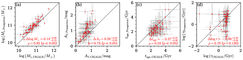
Figure 11: Comparison of SED fitting results with two different SED fitting codes. Panels (a) to (d) compare the estimated $\log M_{*}$, $A_{V}$, $t_{\rm age}$, and $\log\tau$. X and Y axis correspond to the result with CIGALE and Prospector. The black dashed line indicates the $x=y$ line. The median and $1\sigma$ confidence level of the difference between the two results (defined as $\Delta={\rm Prospector}-{\rm CIGALE}$) and Spearman’s correlation coefficient are shown in the lower right part in each panel.

5 $M_{\rm BH}-M_{*}$ relation

In the left panel of Figure 12, we plot our measurements of $M_{\rm BH}$ as a function of $M_{*}$. Based on the large sample covering a broad range in both parameters, we are able to fit the observational data with a linear function and find a positive correlation with a Spearman’s correlation coefficient of $\rho=0.40$. The red line represents the results of a linear fit as given here.

$$\log M_{\rm BH}=\alpha\log M_{*}+\beta,$$ (10)

with $\alpha\simeq 0.67^{+0.21}_{-0.21}$, $\beta\simeq 1.31^{+2.27}_{-2.24}$ and the orange-shaded region showing the $1\sigma$ confidence interval.

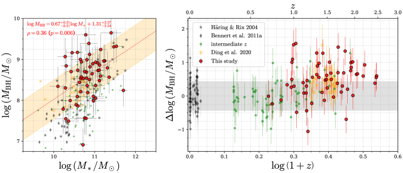
Figure 12: (left) Observed $M_{\rm BH}$ and $M_{*}$ distribution as shown by the red circles. A linear fit is indicated by the red line with the shaded region indicating the $1\sigma$ confidence range. The best-fit relation and Spearman’s correlation coefficient are reported at the top of the panel. (right) $\Delta\log\left(M_{\rm BH}/M_{\odot}\right)$ as a function of redshift where zero corresponds to the local relation as marked by the gray band having a width representing the local dispersion. In both panels, samples from previous studies using HST are plotted: gray for low-$z$ (Häring & Rix, 2004; Bennert et al., 2011b), green for intermediate-$z$ (Jahnke et al., 2009; Bennert et al., 2011a; Cisternas et al., 2011; Schramm & Silverman, 2013) and orange indicating those from Ding et al. (2020) at $z\sim 1.5$.

For comparison, we also provide the linear fit to the local sample consisting of 30 inactive galaxies (Häring & Rix, 2004) and 25 active galaxies (Bennert et al., 2011b). The fit to these 55 galaxies results in $\alpha_{\rm local}\simeq 0.97^{+0.10}_{-0.11}$ and $\beta_{\rm local}\simeq-2.48^{+1.15}_{-1.11}$. Note that the local sample and our high-$z$ sample have different selection effects. Thus, we cannot directly compare $\alpha$ and $\beta$ with $\alpha_{\rm local}$ and $\beta_{\rm local}$ (see Sections 5.1 and 5.2 for the discussion with consideration of selection bias).

For investigating the redshift dependence of the mass relation, we calculate $\Delta\log\left(M_{\rm BH}/M_{\odot}\right)$, the relative offset of the black hole mass at given $M_{*}$ from the local relation:

$$\Delta\log\left(M_{\rm BH}/M_{\odot}\right)=M_{\rm BH}-\alpha_{\rm local}\log\left(M_{*}/M_{\odot}\right)-\beta_{\rm local},$$ (11)

For $\alpha_{\rm local}$ and $\beta_{\rm local}$, we use the above values from the local samples (Häring & Rix, 2004; Bennert et al., 2011b), i.e., $0.97$ and $-2.48$, respectively. We plot $\Delta\log\left(M_{\rm BH}/M_{\odot}\right)$ as a function of $z$ in the right panel of Figure 12. We then parameterize $\Delta\log\left(M_{\rm BH}/M_{\odot}\right)$ to evolve with $z$ as:

$$\Delta\log\left(M_{\rm BH}/M_{\odot}\right)=\gamma\log\left(1+z\right).$$ (12)

Here, we assume there is no redshift change in $\alpha$ and $\beta$ and $\Delta\log M_{\rm BH}$ can be described by only the evolution from the local relation ($\log M_{\rm BH}=\alpha_{\rm local}\log M_{\rm*}+\beta_{\rm local}$). Fitting our data with Equation (12) without considering the selection bias results in $\gamma=1.19^{+0.17}_{-0.15}$, suggesting positive evolution. However, because our sample is (X-ray) flux-limited, it’s essential to consider the impact of selection bias when determining the mass relation (Ding et al., 2020; Li et al., 2021, 2021, e.g.,). Thus, for the rest of this section, we measure the intrinsic slope of the mass relation ($\alpha$) at $z\sim 1.5$ and the redshift evolution parameter ($\gamma$) by comparing our results with mock catalogs as described in Section 3.6. This approach allows us to account for selection bias and measurement uncertainties to determine the intrinsic redshift evolution and dispersion of the mass relation.

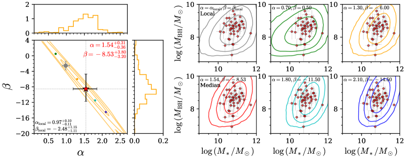
Figure 13: (left) Posterior distribution in the $\alpha-\beta$ plane obtained through a comparison between mock observation and our sample. The posterior distributions for $\alpha$ and $\beta$ are shown in the right and upper 1D histogram. Each contour indicates $1$, $2$, and $3\sigma$ levels. The median and $1\sigma$ confidence levels of $\alpha$ and $\beta$ are shown in the top-right corner of each panel. (right) Comparison of mock observed masses generated with each $\alpha$ and $\beta$ at $z=1.5$ with the real observed data at $z=1-2$ shown in red circles. Contours show the distribution of mock observation, indicating $1$, $2$, and $3\sigma$ levels. Each parameter set, $\alpha$ and $\beta$, is shown in the upper left corner of each panel. As shown, we cannot reject the scenario that $\alpha$ does not evolve up to $z\sim 2.5$.

5.1 Intrinsic slope ($\alpha$) of the mass relation at $z\sim 1.5$

Past efforts to establish the evolution of the ratio between black hole and galaxy mass assume that there is a linear relation at higher redshifts and the slope of the relation matches the local relation (e.g., Ding et al., 2020; Li et al., 2021). This may not necessarily be the case. Here, we assess how well the parameters of a linear relation can be constrained.

In particular, we initially assumed that $\alpha$ and $\beta$, for constructing the mock samples (Equation (9), have constant values independent of the redshift, and the evolution is expressed simply as $\gamma\log\left(1+z\right)$. However, the results in the previous Section 5 may indicate a different $\alpha$ from the local value without considering selection biases. In this section, we examine whether the constant $\alpha$ assumption is valid by estimating the intrinsic value of $\alpha$ while considering selection bias and provide evidence for an intrinsic relation between $M_{\rm BH}$ and $M_{*}$ at $z>1$ for the first time.

Since the parameters $\alpha$, $\beta$, and $\gamma$ exhibit degeneracies, we constrain the $z$ range to $z=1-2$ and perform fitting for $\alpha$ and $\beta$ with an assumption of $\gamma=0$ over this redshift range. Consequently, we cannot compare the estimated $\beta$ with the values in the local relation directly. For the intrinsic dispersion of the mass relation $\sigma_{\mu}$, we assume 0.3 dex, thus matching local studies.

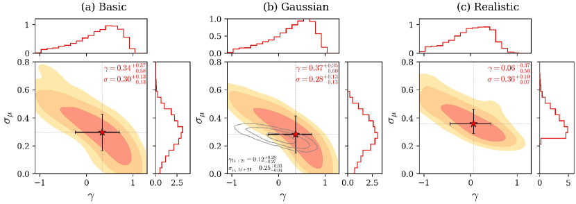
Figure 14: Posterior distribution on the $\sigma_{\mu}-\gamma$ plane obtained through a comparison between mock observation and our sample (the result with the top-5 stacked PSFs). Panels (a) to (c) correspond to the result using basic, Gaussian, and realistic prior settings, respectively. The posterior distribution for $\sigma_{\mu}$ and $\gamma$ are shown in the right and upper 1D histogram. Each contour (red to orange) indicates $1$, $2$, and $3\sigma$ from inner to outer. The median and $1\sigma$ confidence levels of $\gamma$ and $\sigma_{\mu}$ are shown in the top-right corner of each panel. Only in panel (b), we plot the contour from Li et al. (2021) in gray, and their $\gamma$ and $\sigma_{\mu}$ estimations are shown in the lower left corner based on SDSS quasars at $0.3<z<0.8$ with Subaru HSC imaging. Regardless of the prior, the results suggest no or mild evolution at $z<2.5$.

With the mock observed data described in Section 3.6, we apply the selection criteria corresponding to our sample (Section 2.3) and compare them with the observed results to constrain the evolution parameters. We assume the observation thresholds as;

$$F_{\rm[2-10~{}keV]} >F_{\rm[2-10~{}keV],lim},$$ (13)

$$FWHM_{\rm line} >1000~{}{\rm km~{}s^{-1}},$$ (14)

where the first and second conditions correspond to the detection limit of the X-ray observation and broad lines for single epoch $M_{\rm BH}$ estimation. As shown in Figure 2 (a), excluding the three objects, all sources in our sample have $F_{\rm[2-10~{}keV]}$ above the XMM-Newton $F_{\rm[2-10~{}keV],lim}$. Note that all of the three targets with $F_{\rm[2-10~{}keV]}$ smaller than XMM-Newton $F_{\rm[2-10~{}keV],lim}$ are targets observed only with Chandra. Therefore, for the 57 sources other than the three targets, we utilized the XMM-Newton $F_{\rm[2-10~{}keV],lim}$, while for the remaining three, we employed the Chandra $F_{\rm[2-10~{}keV],lim}$; i.e., we changed $F_{\rm[2-10~{}keV],lim}$ depending on the compared observation galaxy. Because $M_{\rm BH}$ of our real targets are based on single epoch estimation with three different lines (${\rm H\alpha}$, ${\rm H\beta}$, and ${\rm Mg{\sc II}}$), we have three different selection thresholds on the mock galaxy using $FWHM_{\rm H\alpha}$, $FWHM_{\rm H\beta}$, and $FWHM_{\rm Mg{\sc II}}$.

For each of our targets, we first select the mock galaxies with the corresponding selection bias, i.e., the selection condition using the same line information used to estimate $M_{\rm BH}$. Furthermore, we select the mock galaxies with a similar redshift; $\left|z-z_{\rm mock}\right|<0.1$. Then, we calculate the probability that the mock galaxies with the similar $z_{\rm mock}$ as the real galaxy would have the same $\tilde{M}_{\rm*,mock}$ with $\left|\Delta M_{\rm*}\right|<0.1$ and $M_{\rm vir,mock}$ with $\left|\Delta M_{\rm BH}\right|<0.1$, i.e., calculate the probability $p$ following

$$p=\frac{N_{\left|\Delta z\right|<0.1,~{}\left|\Delta M_{*}\right|<0.1,~{}\left|\Delta M_{\rm BH}\right|<0.1}}{N_{\left|\Delta z\right|<0.1}}.$$ (15)

We then calculate the likelihood of our sample being observed for each parameter combination of $\alpha$ and $\beta$. Thereby, we estimate the probability distribution of these parameters using MCMC. In the sampling, we assume a uniform prior between 0.1 to 3 for $\alpha$, and -25 to 8 for $\beta$.

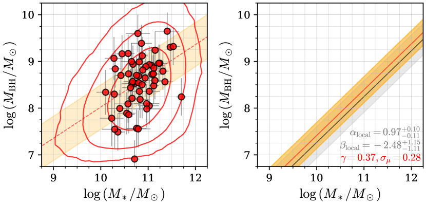
Figure 15: (left) Comparison of the observed sample and the mock observation of $z\sim 1.5$ AGN on the $M_{\rm BH}-M_{*}$ plane. The mock data at $z\sim 1.5$ is constructed with the best-fit $\gamma$ and $\sigma_{\mu}$ (the result with the top-5 stacked PSFs assuming the “Gaussian” prior) while assuming $\alpha_{\rm local}$ and $\beta_{\rm local}$. Small red circles with error bars and the red dashed lines indicate the observed data and the linear fit results (same with Figure 12 left). Contours indicate a distribution of mock observed samples, showing $1$, $2$, and $3\sigma$ from inner to outer. (right) Comparison of the intrinsic $M_{\rm BH}$–$M_{*}$ relation at $z\sim 1.5$ (the red line) to the local relation (the gray line).

The obtained $\alpha-\beta$ distribution is shown on the left panel of Figure 13, indicating a strong anti-correlated degeneracy between $\alpha$ and $\beta$. Because the $1\sigma$ contour includes values $\left(\alpha_{\rm local},\beta_{\rm local}\right)$ corresponding to the local relation, our results do not definitively reject the scenario where $\alpha$ and $\beta$ do not evolve compared to the local relation up to $z\sim 2.5$. However, our results have a preference to higher $\alpha$ than the local relation with $\alpha=1.54^{+0.31}_{-0.36}$. This result suggests high-$z$ mass relation is steeper than the local relation for massive ellipticals, being more consistent with quasar host galaxies at $z\lesssim 0.35$ (Zhuang & Ho, 2023). In the right panels of Figure 13, we show the $M_{\rm BH}-M_{*}$ distribution for mock observed galaxies (similar to Figure 6f) generated with manually sampled parameters on the ridge of the $\alpha-\beta$ degenerated relation and the real observed galaxies ($\alpha\sim 0.7-2.1$). The plots suggest that the mock data exhibits a similar distribution to our sample within the comparable mass range. However, because these parameters are constrained only with our results, more significant differences in $M_{*}$ distribution between the shown parameters become evident at the lower $M_{\rm BH}$ range ($\log\left(M_{\rm BH}/M_{\odot}\right)<8$). Therefore, to break this degenerate relation and improve the precision of determining $\alpha$ and $\beta$, a larger sample with a wider $M_{\rm BH}$ range in future studies is essential.

Even so, we demonstrate that a relation between $M_{\rm BH}$ and $M_{*}$ at high-$z$ is realized based on having a statistical sample afforded by the COSMOS-Web data set. As indicated by Figure 8 (d), the difference in the PSF reconstruction methods does not significantly affect the $M_{*}$ estimation. Therefore, the posterior distribution of $\alpha$ and $\beta$ that are estimated based on $M_{*}$ also shows no significant PSF dependency.

5.2 Intrinsic evolution ($\gamma$) of the $M_{\rm BH}/M_{*}$ relation

To determine the evolution of mass relation with consideration of the selection bias and measurement uncertainties, we generate mock observed catalogs with free parameters of $\gamma$ (evolution rate) and $\sigma_{\mu}$ (intrinsic dispersion of the mass relation) and constrain them by comparing the mock catalogs with observational data in a similar manner to Section 5.1. In contrast to Section 5.1, we fixed $\alpha$ and $\beta$ in Equation (9) to the values in the local relation ($\alpha_{\rm local}$, $\beta_{\rm local}$) to consider the redshift evolution. As illustrated in Section 5.1, we cannot rule out the possibility for evolution of $\alpha$. However, as described in Section 5.1, $\alpha$, $\beta$, and $\gamma$ are strongly degenerate, and obtaining physically meaningful results is challenging when all three parameters are left free for the sample being considered here.

There is still a possibility that $\sigma_{\mu}$ depends on redshift. Nevertheless, as discussed later, imposing strong constraints on $\sigma_{\mu}$ in our results is challenging due to the sample size and its uncertainties. Therefore, we set $\sigma_{\mu}$ as a constant independent of redshift in the fitting. It means $\sigma_{\mu}$ obtained through this method is considered to be an averaged value over $z\sim 0.7-2.5$. Even so, this $\sigma_{\mu}$ estimation has the highest statistical significance for such a study at $z\gtrsim 1$. We discuss the redshift evolution of $\sigma_{\mu}$ in Section 6.2. Finally, in this analysis, we assume no redshift-dependent parameters among the free parameters. Therefore, there is no need to restrict the redshift range within the data, as in Section 5.1.

In the fitting process, we assume a uniform prior distribution for $\gamma$ between $-1<\gamma<1$. Then, we have three different prior settings for $\sigma_{\mu}$: a uniform distribution between $0.01<\sigma_{\mu}<1.0$ (basic), a Gaussian distribution with a mean of 0.3 dex and a standard deviation of 0.1 dex (Gaussian), and a uniform distribution between $0.25<\sigma_{\mu}<1.0$ with a prohibition of $\sigma_{\mu}<0.25$ (realistic).

Figure 14 shows the estimated posterior distributions of $\gamma$ and $\sigma_{\mu}$ using each prior setting with the top-5 stacked PSF results. As evident in all panels by the orange contours, the intrinsic dispersion $\sigma_{\mu}$ is strongly degenerate with the evolution rate $\gamma$ where a smaller $\gamma$ results in a larger $\sigma_{\mu}$ as demonstrated in previous studies (Ding et al., 2020; Li et al., 2021). To reiterate, a smaller value for $\gamma$ biases the mass relation towards relatively lower $M_{\rm BH}$ values thus a larger $\sigma_{\mu}$ is required to reproduce a certain set of observation data.

Considering the likelihood distribution for $\gamma$, the “basic” prior setting shows a slight positive-to-no evolution with $\gamma=0.34^{+0.37}_{-0.58}$. Similarly, the “Gaussian” prior setting results in $\gamma=0.37^{+0.35}_{-0.60}$, just slightly closer to the case of ”no evolution ($\gamma=0$). If we assume that the intrinsic dispersion should not be significantly smaller than the local dispersion, we limit the allowed range for $\sigma_{\mu}$ to be above $0.25$ (”Realistic” case). In this case, we find $\gamma=0.06^{+0.37}_{-0.50}$, remarkably close to the case for no evolution. For the latter, the intrinsic dispersion is slightly higher at $0.36^{+0.10}_{-0.07}$. In all cases, our results are consistent with very mild or essentially a lack of evolution with respect to the local relation.

Then, the left panel of Figure 15 compares mock observations using the median parameters ($\gamma=0.30$ and $\sigma_{\mu}=0.29$) under the assumption of “Gaussian” prior with the actual observational $M_{\rm BH}$–$M_{*}$ distribution and relation. We can see that the mock data can explain the observed data well. The right panel of Figure 15 compares the intrinsic relationship, i.e., the relation corrected for the selection bias, with the local relation. Again, the resulting intrinsic relation is consistent with the local relation within the range of errors.

6 Discussion

In Section 5.2, our findings suggest a mild or lack of evolution of the mass relation from the local relation when considering selection biases and measurement uncertainties. In this section, we first compare the derived values of $\gamma$ and $\sigma_{\mu}$ from Section 5.2 with previous studies. Then, we also discuss the cosmic averaging scenario (Peng, 2007; Hirschmann et al., 2010; Jahnke & Macciò, 2011).

6.1 Comparison to other studies

First, the conclusion of no or mild evolution with $\gamma=0.37^{+0.35}_{-0.60}$ is consistent with studies based on 2D decomposition analysis (e.g., Ding et al., 2020; Li et al., 2021) and studies using a SED-fitting-based decomposition method (e.g., Sun et al., 2015; Suh et al., 2020).

In Figure 14, we compare our results on the estimated $\gamma-\sigma_{\mu}$ distribution to those of Li et al. (2021). Our sample has higher redshift range than Li et al. (2021), and the change of $\Delta\log\left(M_{\rm BH}/M_{\odot}\right)$ is also proportional to $\log\left(1+z\right)$ in our model. Therefore, to reproduce the observational results, when increasing $\gamma$, we need to decrease $\sigma_{\mu}$ more than Li et al. (2021). In other words, the slope of the $\gamma$–$\sigma_{\mu}$ degenerate relation is steeper in our study. As a result, while the sample size of this study is approximately ten times smaller than Li et al. (2021), the uncertainty of $\gamma$ is only $\sim 2$ times larger than Li et al. (2021). On the other hand, due to the steep slope, imposing constraints on $\sigma_{\mu}$ becomes challenging, and the uncertainty becomes $\sim 4$ times larger than Li et al. (2021). Even so, our estimated value of $\sigma_{\mu}$ is $0.28^{+0.13}_{-0.13}$, which is remarkably similar to Li et al. (2021) with $\sigma_{\mu}$=$0.25_{-0.04}^{+0.03}$.

It is worth highlighting that the inference on the value of $\gamma$ is very close to zero for the ”Realistic” case (Fig. 14c) where we assume that the intrinsic scatter ($\sigma_{\mu}$) cannot be lower than the local dispersion. Interestingly, if $\sigma_{\mu}$ ($\sim 0.4-0.5$) is actually higher than the local value, this would push the evolution parameter to negative values ($\gamma\sim-0.5$) thus presenting a scenario where the black holes have to catch up to their host galaxies by a bit.

6.2 Scatter ($\sigma_{\mu}$) evolution and cosmic averaging

When assuming a non-casual cosmic averaging scenario (Jahnke & Macciò, 2011), major mergers average and equalize the mass ratio $M_{\rm BH}/M_{*}$ through cosmic history. Thus, $\sigma_{\mu}$ should increase towards high redshift.

To test the cosmic averaging scenario with our data, we generate a mock sample (20,000 parameter sets of $M_{\rm BH}$ and $M_{*}$) at $z\sim 1.4$, the median redshift of our observational sample. We generate $M_{*}$ based on the SMF by Weaver et al. (2023), and calculate the $M_{\rm BH}$ assuming the $\gamma$ and $\sigma$ sampled in the MCMC run with “Gaussian” prior setting (Section 5.2). Each mock galaxy is assumed to undergo major mergers following the major merger rate from Rodriguez-Gomez et al. (2015) covering $z\sim 0-1.4$. We simulate the redshift evolution of $M_{\rm BH}$ and $M_{*}$ by summing them with those of merging partners. Then, we calculate $\sigma_{\mu}$ at each redshift to trace the expected scatter evolution from the assumed conditions. In this simulation, we do not consider the accretion onto the black hole and star formation, i.e., both $M_{\rm BH}$ and $M_{*}$ are assumed to grow only through major mergers. We limit the mergers to those with mass ratios within $\pm 0.5~{}{\rm dex}$.

Figure 16 compares the simulated redshift evolution of $\sigma_{\mu}$ with the results from this study and Li et al. (2021). When assuming the evolution only through major mergers, the growth within the $1\sigma$ uncertainty range significantly encompasses the results of Li et al. (2021). Moreover, our median redshift evolution is consistent with the results of Li et al. (2021). Therefore, the $\sigma_{\mu}$ difference between the results from this study and Li et al. (2021) could be interpreted as the major merger-based scatter evolution.

However, due to the large uncertainty in our results, we cannot draw any definitive conclusions regarding the redshift evolution of $\sigma_{\mu}$. Furthermore, as evident from Figure 16, our sample has a wide redshift range compared to Li et al. (2021). If $\sigma_{\mu}$ varies with redshift, the sample should be binned in a narrower redshift range to trace the redshift evolution. Nevertheless, as mentioned in Sections 5.1 and 5.2, the degeneracy relation on the $\gamma-\sigma_{\mu}$ plane tends to steepen toward higher redshifts, making it relatively challenging to impose constraints on $\sigma_{\mu}$. Future high-$z$ statistical studies will likely require samples of a similar size to Li et al. (2021) with $N=584$, or even larger to address the redshift evolution of $\sigma_{\mu}$. Thus, it will be necessary to conduct comprehensive surveys of high-$z$ AGNs using next-generation survey data such as Euclid and Roman.

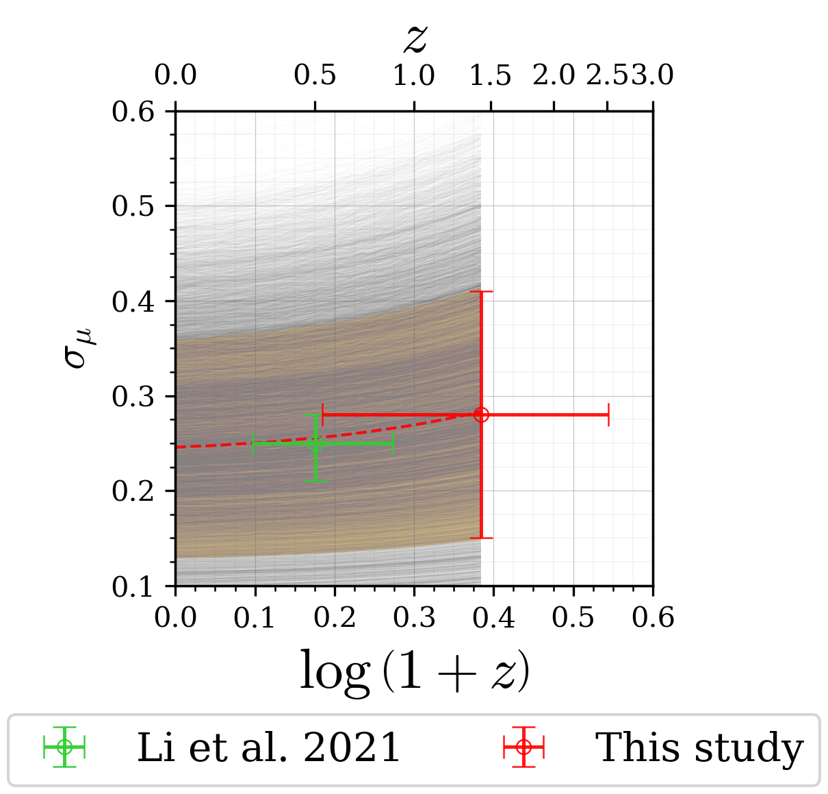
Figure 16: Evolution of $\sigma_{\mu}$ at $z\lesssim 2$ based on a simple simulation of the cosmic averaging scenario. The vertical red error bars represent the scatter in $\sigma_{\mu}$ within the $z$ range of our sample using the basic prior. Faint grey lines correspond to each sampled parameter set while the red line and the orange filled region represent the median and 1$\sigma$ confidence level of $\sigma_{\mu}$ redshift evolution. The green data denotes the constraint from Li et al. (2021) which is consistent within the $1\sigma$ range of our results.

6.3 General notes on PSF reconstruction methods

So far, various studies have performed decomposition of JWST images (e.g. Ding et al., 2022a, 2023; Stone et al., 2023; Yue et al., 2023; Harikane et al., 2023; Zhuang & Shen, 2023; Zhuang et al., 2023; Stone et al., 2023). As discussed above or in the previous studies, the results of the AGN+host galaxy 2D decomposition depend significantly on the PSF reconstruction. Especially, Zhuang & Shen (2023) discussed the effect of different PSF on decomposition results. Zhuang & Shen (2023) compared three PSF modeling methods (SWarp, photutils, and PSFEx), but they did not compare them with $\chi^{2}_{\nu}$ based methods directly. Thus, in this paper, we summarize the comparison when using different PSF reconstruction methods.

In this study, we compare three final PSFs: two obtained by $\chi^{2}_{\nu}$-based methods (a top-5 stacked PSF and a top-75% stacked PSF) and one from an empirically modeling method, PSFEx. As demonstrated in Figure 4, we find offsets in FWHM among different PSF reconstruction methods. These PSF variations, as indicated by Zhuang & Shen (2023), could potentially introduce biases in estimating $n$, $r_{e}$, or $H/T$. This is due to a broader (narrower) PSF than in reality which tends to result in smaller (larger) $n$, larger (smaller) $r_{e}$, and overestimation of host fluxes. However, as shown in Figure 8, morphological parameters such as $n$, $r_{e}$, $H/T$ generally exhibit consistent relations. Besides, as shown in Figure 8 (d), different PSFs have less impact on $M_{*}$ estimation than on $H/T$. This could be due to the fact that $M_{*}$ is estimated from SED fitting (Section 3.5) using multi-band photometry that averages the uncertainty in each band. If so, SED fitting with a smaller number of photometric bands (e.g., Ding et al., 2023; Yue et al., 2023), may lead to more severe effects from inaccurate PSF reconstruction. We also find each method has advantages and disadvantages from a technical aspect. Lastly, we summarize below the technical comparison between each method.

Modeling method: The approach of constructing an empirical PSF model from numerous stars, such as PSFEx in this study, has the advantage of being less influenced by noise compared to the $\chi^{2}_{\nu}$-based methods, as depicted in Figure 17. This method also allows flexible modeling, considering PSF as a function of position or brightness.

However, a drawback is the requirement for many PSF candidates to model a local or flux-dependent PSF, which can be considered a trade-off. Furthermore, we also confirm that FWHM values of PSFEx PSFs depend on configuration parameters. When reconstructing PSFs, it is challenging to determine the best configuration parameters because the exact PSFs are not known.

$\chi^{2}_{\nu}$-based selection method: Selecting PSFs based on $\chi^{2}_{\nu}$ from a substantial number of stars, such as Top-5 or Top-75% PSFs, allows easy analysis considering the PSF uncertainties. Also, by fitting with various different single PSFs, the possibility for PSF mismatches is minimized. Notably, Yue et al. (2023) discussed the differences in broad-band PSFs attributed to variations in SED shapes between stars and AGNs. Our method using all single PSFs in the PSF library may consider this PSF uncertainty as a result of selecting low-$\chi^{2}_{\nu}$ single PSFs with a matched shape.

However, using fewer PSF candidates, like the top-5 stacked PSF, might increase the noise of the final PSF, as observed in Figure 17. Note that this noise is generally smaller than the central main component; thus, it should not affect significantly except in the case with small $H/T$. Additionally, our approach involves visual inspection in PSF candidate selection, which might cause a bias. Also, as mentioned by Zhuang & Shen (2023), a lower $\chi^{2}_{\nu}$ does not necessarily mean more correct PSF. Moreover, as a practical demerit, this method needs more time to create a PSF library with visual inspection in each filter and region and more computational cost for SED fittings with all single PSFs.

Given that we do not know the correct answers in this study, it is challenging to discuss which method produces the most accurate results. For some targets, decomposition is clearly successful with one final PSF, which can then be evaluated from the residual emission based on other PSFs. We also confirm that these failures in fitting can occur with all final PSFs. Therefore, we conclude that it is best to assess the impact on derived properties (e.g., $n$, $r_{e}$, $H/T$) by varying the method of PSF construction (Section 3.1) and place equal weight on assessing the uncertainties based on varying PSFs (Section 3.3) to obtain solid 2D decomposition results.

7 Conclusions

We performed a 2D decomposition analysis of high-$z$ ($z\sim 0.7-2.5$) type-I AGNs using the COSMOS-Web (Casey et al., 2023) and PRIMER-COSMOS surveys to measure the black hole – stellar mass relation at high-$z$. Our sample contains 61 targets that are X-ray-selected, broad-line AGNs with single-epoch black hole mass estimates ($\log\left(M_{\rm BH}/M_{\odot}\right)\sim 7.5-9.5$) based on ${\rm H}\beta$, ${\rm H}\alpha$, and Mgii from previous spectroscopic surveys (e.g., Schulze et al., 2018).

By utilizing HST/ACS + JWST/NIRCam imaging that covers the rest-frame optical to near-infrared, we obtained multi-band information of the AGN host galaxies with unprecedented spatial resolution in which we can clearly identify substructures such as bars and spirals arms (Figure 9). Since AGN–host 2D decomposition is known to be sensitive to the PSF reconstruction methods, we compared the results with three final PSFs reconstructed using the modeling method PSFEx and a $\chi^{2}_{\nu}$-based selection method. Through a meticulous decomposition analysis using various PSFs, we successfully detected the host galaxies in more than two filters for $\sim 90\%$ of the entire sample. Then, we confirmed that host morphological parameters such as $n$, $r_{e}$, and $H/T$ remain relatively consistent regardless of the PSF reconstruction method used (Figure 8). Furthermore, given the high quality of the host galaxy images, this study is expected to serve as a crucial stepping stone for image-based spatially-resolved investigations of AGN host galaxies, such as double-Sérsic model fitting (decomposition fitting with AGN, bulge, and disk components) or parametric/non-parametric substructure analysis.

With AGN-subtracted photometry of the host galaxy in multiple bands, we estimated $M_{*}$ by performing SED fitting and present the $M_{\rm BH}$–$M_{*}$ relation at $z\sim 0.7-2.5$ (Figure 12). There is a positive correlation between $M_{\rm BH}$ and $M_{*}$ with the correlation coefficient of $\rho=0.36$ ($p\ll 0.05$). We fit the mass relation by a simple (log-)linear relation of $\log\left(M_{\rm BH}/M_{\odot}\right)=\alpha\log\left(M_{*}/M_{\odot}\right)+\beta$ with consideration of selection biases and measurement uncertainties. Our results show that the slope of the mass relation at $z\sim 2$ ($\alpha=1.54^{+0.31}_{-0.36}$) is slightly steeper than yet consistent with the local relation ($\alpha_{\rm local}=0.97^{+0.10}_{-0.11}$) (Figure 13).

Assuming the redshift evolution term of the mass relation to be $\gamma\log\left(1+z\right)$, we further determine the evolution factor $\gamma$ and the intrinsic scatter of the mass relation $\sigma_{\mu}$ while considering selection biases and uncertainties based comparisons to mock catalogs (Figure 14). Even though the estimated probability distribution shows strong degeneracy between $\gamma$ and $\sigma_{\mu}$, we find no or mild evolution with $\gamma=0.37^{+0.35}_{-0.60}$. The estimated $\gamma-\sigma_{\mu}$ distribution is largely consistent with Li et al. (2021) based on the HSC imaging of SDSS quasars at $z<0.8$. Given the higher redshift range of our sample, the slope of the degeneracy relation between $\gamma$ and $\sigma_{\mu}$ is steeper than Li et al. (2021). Therefore, despite the sample being $\sim 10$ times smaller, the estimated $\gamma$ uncertainty is just slightly larger than Li et al. (2021).

Furthermore, the estimated value of the intrinsic scatter is $\sigma_{\mu}=0.28^{+0.13}_{-0.13}$ which is consistent with the local relation and the recent estimate by Li et al. (2021). We show that this value $\sigma_{\mu}$ at high-z may not be in contradiction to a cosmic averaging scenario (Figure 16) as recently put forward by Li et al. (2021) and Ding et al. (2022b) where AGN feedback is invoked to explain the constant level of dispersion with redshift. However, due to the small sample size, high redshift, and wide redshift range, our constraints on the redshift evolution of $\sigma_{\mu}$ are weak. Thus, a larger sample size at $z\sim 1-3$ is needed, especially at high-$z$.

Future large-scale surveys such as Euclid and Roman will significantly augment the sample size, along with deeper observations by JWST, to provide stronger constraints on SMBH and galaxy evolution. For future large imaging data sets, visual inspection for all multi-component fits and manually exclusion of anomalous results will not be feasible; thus, improvements in 2D decomposition techniques or the imposition of more sophisticated conditions to confirm the robustness of host detection is needed. In order to address these challenges, it is imperative to enhance the 2D decomposition analysis by mitigating the uncertainties related to PSF reconstruction. This involves conducting a meticulous analysis of AGN PSFs, determining the validity of applying stellar PSFs to AGN with different SEDs than stars, identifying the most effective methods for accurate PSF reconstruction, and establishing a framework for evaluating the uncertainties in reconstructed PSFs.

Appendix A Detected numbers in each filters

Table 4 summarizes the number of undetected host galaxies based on the conditions described in Section 3.3 for each PSF and filter, while Table 5 then summarizes the number of detected hosts for each final PSF. Regarding the JWST filters, we have less galaxies that are classified as non-detection due to the ${\rm BIC}$ condition than due to the $S/N_{\rm host}$ condition. The number of undetected hosts is lowest in F277W, followed by F150W and F444W. On the other hand, F115W and F814W show a larger number of undetected hosts, especially due to $S/N_{\rm host}$. This trend is because F814W is the HST observation with lower resolution and shallower depth than the JWST observations, and both F814W and F115W are in the shorter-wavelength side of the Balmer break, leading to a tendency for a smaller intrinsic $H/T$.

Table 4: The number of the undetected host galaxies for each condition, PSF and filter

		(1)	(2)	(3)
Filter	PSF	BIC	$S/N$	manual	Total
F814W	Top-5	14	22	17	39
	Top-75%	14	21	17	38
	PSFEx	21	24	17	41
F115W	Top-5	2	11	1	12
	Top-75%	1	10	1	11
	PSFEx	7	10	1	12
F150W	Top-5	1	2	1	3
	Top-75%	2	3	1	5
	PSFEx	2	3	1	4
F277W	Top-5	0	0	1	1
	Top-75%	0	0	1	1
	PSFEx	0	1	1	2
F444W	Top-5	0	2	2	4
	Top-75%	0	2	2	4
	PSFEx	0	1	2	3

Table 5: The number of host-galaxy detections for each final PSF

	# Detected filters
PSF	COSMOS-Web						PRIMER
	0	1	2	3	4	5	9
Top-5	1	0	5	9	27	16	3
Top-75%	1	2	4	6	28	17	3
PSFEx	2	0	4	8	30	14	3

Appendix B Detailed comparison of different PSF results

As mentioned in Section 3.1, 2D decomposition is significantly influenced by the differences in PSFs. In this study, we compare three different PSFs and discuss the PSF dependency of the results. Figure 17 (images on the left; a–c) shows each final PSF image for the four NIRCam filters. We fit each final PSF and each single PSF in the PSF library with the 2D Gaussian model, and measure the FWHM along a semi-major axis and ellipticity $b/a$ (defined as $FWHM_{\rm minor}/FWHM_{\rm major}$). Figures 17 (d) and (e) show the distribution of FWHM and $b/a$ in each filter for an example AGN, CID-62, with $z_{\rm spec}\sim 1.92$. As the number of stars used increases in the order of the top-5 stacked, the top-75% stacked, and PSFEx, we can see that the background noise is correspondingly lower. Regarding the FWHM distribution, the top-5 and the top-75% PSFs are consistent with the FWHM distributions of single PSFs within the PSF library. PSFEx have consistent FWHMs in F115W and F150W, and slightly smaller FWHMs in F277W and F444W, suggesting the possibility of bias between automatic PSF selection by PSFEx and semi-automatic PSF selection by galight. In addition, each final PSF tends to have a higher $b/a$ than individual single PSFs. Regardless of whether $\chi^{2}_{\nu}$-based stacking or empirical modeling is employed, considering that the final PSF is a more reasonable PSF reconstruction than a single PSF, this suggests a potential bias towards a more elliptical PSF when using a single PSF. Next, Figure 18 compares the estimated $H/T$ using each PSF and filter (the full-filter version of Figure 8 (c)). We can find strong positive correlations for all filters, with the distribution along the $y=x$ relation. However, when comparing the distribution with $y=x$, it is evident that PSFEx tends to estimate larger $H/T$ for F277W and F444W compared to top-5 and top-75% PSFs. As mentioned in Section 4.2, this trend can be interpreted by considering the differences in FWHM for each filter and PSF. As shown in Figure 4, PSFEx tends to exhibit smaller PSFs in F277W and F444W than the top-5 and top-75% PSFs. Zhuang & Shen (2023) suggest that different PSFs result in larger $H/T$ in the 2D decomposition analysis. Therefore, it is conceivable that PSFEx shows larger $H/T$ in F277W and F444W with the smaller PSFs than the top-5 and top-75% PSFs.

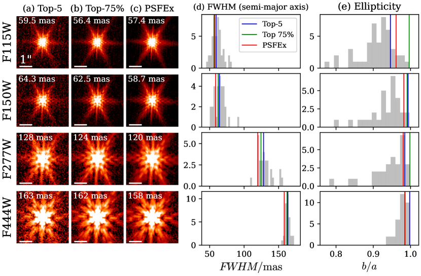
Figure 17: Comparison of different methods to evaluate empirical models of the PSF. Columns (a) to (c) show images of the top-5 stacked PSF, the top-75% stacked PSF, and the PSFEx-PSF for an example galaxy, CID-62 ($z=1.92$), in F115W, F150W, F277W, and F444W, from top to bottom. FWHM along the semi-major axis measured from the 2D Gaussian fits shown in the top-left corner of each image. The white bars in the lower left indicate a scale of $1^{\prime\prime}$. Columns (d) and (e) show the distribution of the FWHM (semi-major axis) and ellipticity $b/a$. Gray histograms display the distribution of each single PSF in the library (Section 3.1.1). The values for the top-5 stacked PSF, the top-75% stacked PSF, PSFEx-PSF are marked by the blue, green, and red vertical lines, respectively.

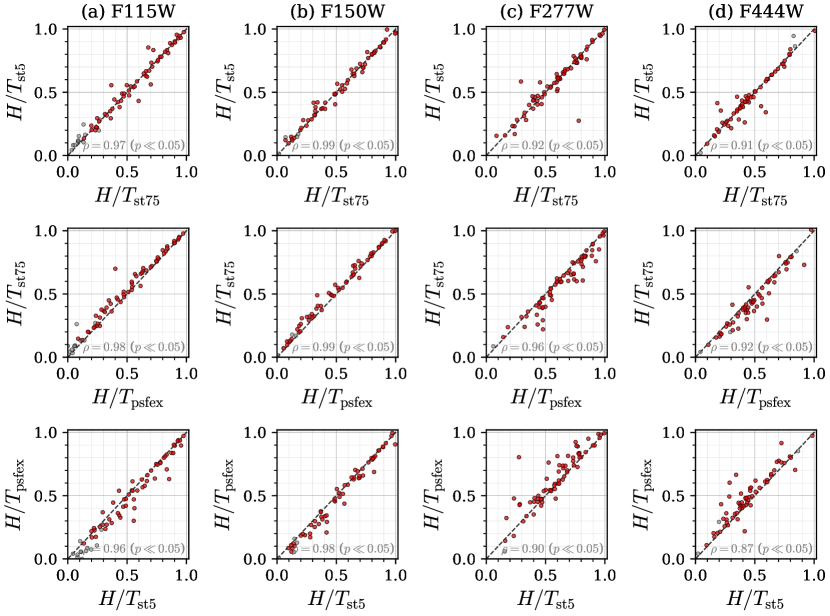
Figure 18: Comparison of the estimated $H/T$ in each filter using different PSFs (Columns (a) to (d)). The gray and red colors correspond to whether they were detected in each filter. Spearman’s correlation coefficient $\rho$ for each prior is shown in the lower right corner of each panel. High correlation coefficients and the distribution around $y=x$ (black dashed line) suggest consistent results among the fitting with different PSFs.

Appendix C galight test with mock image

We generate mock images of AGN and their host galaxies and perform 2D decomposition on these images to verify whether galight can accurately recover each parameter for the host galaxies. We use lenstronomy (Birrer & Amara, 2018; Birrer et al., 2021) to generate 2,000 NIRCam/F150W mock galaxy images. These are constructed as a superposition of a PSF and a smooth analytic Sérsic model based on randomly sampled parameters: host-to-total flux ratio ($H/T$), Sérsic index ($n$), effective radius ($r_{e}$), semi-major axis orientation ($\theta$), and ellipticity ($b/a$). The software tools lenstronomy and galight have different definitions of $r_{e}$, with the relation $r_{e,{\rm galight}}=\left(b/a\right)^{-0.5}\times r_{e,{\rm lenstronomy}}$. In this section and consistent with the main part of this paper, all $r_{e}$ are unified under the definition in galight. The specified range for each parameter is $\log(H/T)$ in $\left[\sim-5,0\right]$, $n$ in $\left[1,6\right]$, $r_{e}$ in $\left[\sim 0\farcs 05,1\farcs 6\right]$, $b/a$ in $\left[0.2,1.0\right]$, and $\theta$ in $\left[0,\pi\right]$ (in radian). We assume the PSFEx PSF (Section 3.1.2) and that the center of host galaxy components are aligned with the center of PSF components. Additionally, we add Gaussian noise equivalent to the real NIRCam/F150W COSMOS-Web images. Using the generated mock images, we performed 2D decomposition with the low-$\chi^{2}_{\nu}$ top-5 PSF reconstruction strategy (Section 3.1.1). Since the PSFEx PSF is assumed when generating the mock images, the results allow us to assess the performance in cases where the PSF may differ from the true PSF, similar to real data analysis. Note that we cannot conclude which PSF reconstruction method is superior from this analysis. In this test, we also cannot consider the effects of more complex morphological features than single Sérsic components, such as double Sérsic (disc+bulge) components, position offset between AGN and host, substructures (bars, spirals, and clumps), and nearby or merging objects. Figure 19 compares the estimated major parameters ($H/T$, $r_{e}$, $n$) with the input values. First, focusing on $H/T$, we can find the distinct change in the trend around the input $\log\left(H/T\right)$ value $\log\left(H/T_{\rm ans}\right)\sim-2$. For $\log\left(H/T_{\rm ans}\right)\lesssim-2$, the estimated value $\log\left(H/T_{\rm est}\right)$ remains relatively constant around $-1.5$, deviating significantly from the $y=x$ line. This implies that detecting weak galaxy components with $\log\left(H/T_{\rm ans}\right)\lesssim-2$ is practically challenging using the 2D decomposition analysis with galight. On the other hand, for $\log\left(H/T_{\rm ans}\right)\gtrsim-2$, $\log\left(H/T_{\rm est}\right)$ exhibits a consistent trend along the $y=x$ relation, while slightly larger than the input values. This trend is consistent with Zhuang & Shen (2023), who reported that different PSFs tend to overestimate $H/T$. As shown in Figure 7, $\log\left(H/T_{\rm est}\right)$ for the real detected galaxies in this study are $\log\left(H/T_{\rm est}\right)\gtrsim-1$. If we limit the mock results to $\log\left(H/T_{\rm est}\right)\gtrsim-1$, the difference between the estimation and input values (defined as estimation - input values) is $\Delta\log\left(H/T\right)\sim 0.06\pm 0.09~{}{\rm dex}$, suggesting sufficiently consistent estimation of $H/T$. Next, examining $r_{e}$ and $n$, we find a consistent distribution along the $y=x$ relation, with an overall tendency to underestimate $r_{e}$ and overestimate $n$. We can also see that some objects hit the $r_{e}$ lower limit ($r_{e}\sim 0\farcs 05$) and $n$ upper limit ($n\sim 9$). If we limit the analysis to the above realistic cases ($\log\left(H/T_{\rm est}\right)\gtrsim-1$), as shown in Figure 19, $r_{e}$ shows consistent results with $\Delta r=-0.1\pm 0.2$ and less hitting to the $r_{e}$ lower limit. However, for $n$, many objects still exhibit the $n$ upper limit even with $\log\left(H/T_{\rm est}\right)\gtrsim-1$. If we additionally cut the upper limit object with $n<8.8$, the difference between the estimation and the input values is $\Delta n\sim 1.3\pm 1.6$, suggesting a consistent estimation with medium scatter. We confirm that larger-$n$ objects tend to have larger $\Delta n$, indicating the increasing difficulty of accurately reconstructing $n$ when they have larger $n$.

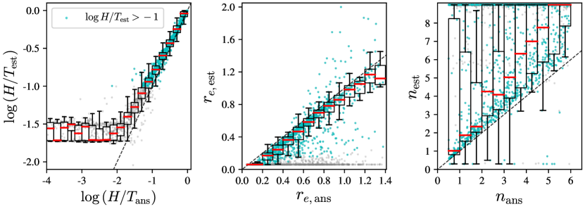
Figure 19: Comparison of input (X-axis) and estimated (Y-axis) morphological parameters of mock galaxies. Columns (a) to (c) compare $\log\left(H/T\right)$, $r_{e}$, and $n$, respectively, and the black dashed line indicate $y=x$. The gray and cyan circles indicate the all mock galaxies and the galaxies with $\log\left(H/T_{\rm est}\right)>-1$ corresponding to the minimum $H/T_{\rm est}$ for our real galaxies (also see Figures 8, 18). Only mock galaxies with $\log\left(H/T_{\rm est}\right)>-1$ are used in plotting box plots for $n$ and $r_{e}$.

References

- Baker et al. (2023) Baker, W. M., Tacchella, S., Johnson, B. D., et al. 2023. http://arxiv.org/abs/2306.02472
- Beifiori et al. (2012) Beifiori, A., Courteau, S., Corsini, E. M., & Zhu, Y. 2012, MNRAS, 419, 2497, doi: 10.1111/j.1365-2966.2011.19903.x
- Bennert et al. (2011a) Bennert, V. N., Auger, M. W., Treu, T., Woo, J.-H., & Malkan, M. A. 2011a, ApJ, 742, 107, doi: 10.1088/0004-637X/742/2/107
- Bennert et al. (2011b) —. 2011b, ApJ, 726, 59, doi: 10.1088/0004-637X/726/2/59
- Bennert et al. (2021) Bennert, V. N., Treu, T., Ding, X., et al. 2021, ApJ, 921, 36, doi: 10.3847/1538-4357/ac151a
- Bertin (2011) Bertin, E. 2011, in Astronomical Society of the Pacific Conference Series, Vol. 442, Astronomical Data Analysis Software and Systems XX, ed. I. N. Evans, A. Accomazzi, D. J. Mink, & A. H. Rots, 435
- Bertin & Arnouts (1996) Bertin, E., & Arnouts, S. 1996, A&AS, 117, 393, doi: 10.1051/aas:1996164
- Birrer & Amara (2018) Birrer, S., & Amara, A. 2018, Physics of the Dark Universe, 22, 189, doi: 10.1016/j.dark.2018.11.002
- Birrer et al. (2021) Birrer, S., Shajib, A., Gilman, D., et al. 2021, The Journal of Open Source Software, 6, 3283, doi: 10.21105/joss.03283
- Boquien et al. (2019) Boquien, M., Burgarella, D., Roehlly, Y., et al. 2019, A&A, 622, A103, doi: 10.1051/0004-6361/201834156
- Bouchet et al. (2015) Bouchet, P., García-Marín, M., Lagage, P.-O., et al. 2015, The Mid-Infrared Instrument for the James Webb Space Telescope, III: MIRIM, The MIRI Imager
- Bradley (2023) Bradley, L. 2023, astropy/photutils: 1.8.0, 1.8.0, Zenodo, Zenodo, doi: 10.5281/zenodo.7946442
- Bradley et al. (2023) Bradley, L., Sipőcz, B., Robitaille, T., et al. 2023, astropy/photutils: 1.8.0, 1.8.0, Zenodo, doi: 10.5281/zenodo.7946442
- Brightman et al. (2013) Brightman, M., Silverman, J. D., Mainieri, V., et al. 2013, MNRAS, 433, 2485, doi: 10.1093/mnras/stt920
- Brusa et al. (2010) Brusa, M., Civano, F., Comastri, A., et al. 2010, ApJ, 716, 348, doi: 10.1088/0004-637X/716/1/348
- Bruzual & Charlot (2003) Bruzual, G., & Charlot, S. 2003, MNRAS, 344, 1000, doi: 10.1046/j.1365-8711.2003.06897.x
- Bushouse et al. (2023) Bushouse, H., Eisenhamer, J., Dencheva, N., et al. 2023, JWST Calibration Pipeline, 1.10.0, Zenodo, doi: 10.5281/zenodo.7795697
- Calzetti et al. (2000) Calzetti, D., Armus, L., Bohlin, R. C., et al. 2000, ApJ, 533, 682, doi: 10.1086/308692
- Cappelluti et al. (2009) Cappelluti, N., Brusa, M., Hasinger, G., et al. 2009, A&A, 497, 635, doi: 10.1051/0004-6361/200810794
- Casey et al. (2023) Casey, C. M., Kartaltepe, J. S., Drakos, N. E., et al. 2023, ApJ, 954, 31, doi: 10.3847/1538-4357/acc2bc
- Cen (2015) Cen, R. 2015, ApJ, 805, L9, doi: 10.1088/2041-8205/805/1/L9
- Chabrier (2003) Chabrier, G. 2003, PASP, 115, 763, doi: 10.1086/376392
- Cisternas et al. (2011) Cisternas, M., Jahnke, K., Bongiorno, A., et al. 2011, ApJ, 741, L11, doi: 10.1088/2041-8205/741/1/L11
- Civano et al. (2012) Civano, F., Elvis, M., Brusa, M., et al. 2012, ApJS, 201, 30, doi: 10.1088/0067-0049/201/2/30
- Collaboration et al. (2022) Collaboration, T. A., Price-Whelan, A. M., Lim, P. L., et al. 2022, The Astrophysical Journal, 935, 167, doi: 10.3847/1538-4357/ac7c74
- Conroy & Gunn (2010) Conroy, C., & Gunn, J. E. 2010, ApJ, 712, 833, doi: 10.1088/0004-637X/712/2/833
- Conroy et al. (2009) Conroy, C., Gunn, J. E., & White, M. 2009, ApJ, 699, 486, doi: 10.1088/0004-637X/699/1/486
- DeGraf et al. (2015) DeGraf, C., Di Matteo, T., Treu, T., et al. 2015, MNRAS, 454, 913, doi: 10.1093/mnras/stv2002
- Di Matteo et al. (2008) Di Matteo, T., Colberg, J., Springel, V., Hernquist, L., & Sijacki, D. 2008, ApJ, 676, 33, doi: 10.1086/524921
- Ding et al. (2022a) Ding, X., Silverman, J. D., & Onoue, M. 2022a. http://arxiv.org/abs/2209.03359
- Ding et al. (2020) Ding, X., Treu, T., Silverman, J. D., et al. 2020, ApJ, 896, 159, doi: 10.3847/1538-4357/ab91be
- Ding et al. (2020) Ding, X., Silverman, J., Treu, T., et al. 2020, The Astrophysical Journal, 888, 37, doi: 10.3847/1538-4357/ab5b90
- Ding et al. (2022b) Ding, X., Silverman, J. D., Treu, T., et al. 2022b, The Astrophysical Journal, 933, 132, doi: 10.3847/1538-4357/ac714c
- Ding et al. (2023) Ding, X., Onoue, M., Silverman, J. D., et al. 2023, Nature, 621, 51, doi: 10.1038/s41586-023-06345-5
- Duras et al. (2020) Duras, F., Bongiorno, A., Ricci, F., et al. 2020, A&A, 636, A73, doi: 10.1051/0004-6361/201936817
- Elvis et al. (2009) Elvis, M., Civano, F., Vignali, C., et al. 2009, ApJS, 184, 158, doi: 10.1088/0067-0049/184/1/158
- Fabian (2012) Fabian, A. C. 2012, ARA&A, 50, 455, doi: 10.1146/annurev-astro-081811-125521
- Ferrarese & Merritt (2000) Ferrarese, L., & Merritt, D. 2000, ApJ, 539, L9, doi: 10.1086/312838
- Garilli et al. (2008) Garilli, B., Le Fèvre, O., Guzzo, L., et al. 2008, A&A, 486, 683, doi: 10.1051/0004-6361:20078878
- Graham et al. (2011) Graham, A. W., Onken, C. A., Athanassoula, E., & Combes, F. 2011, MNRAS, 412, 2211, doi: 10.1111/j.1365-2966.2010.18045.x
- Greene et al. (2023) Greene, J. E., Labbe, I., Goulding, A. D., et al. 2023, arXiv e-prints, arXiv:2309.05714, doi: 10.48550/arXiv.2309.05714
- Gültekin et al. (2009) Gültekin, K., Richstone, D. O., Gebhardt, K., et al. 2009, ApJ, 698, 198, doi: 10.1088/0004-637X/698/1/198
- Habouzit et al. (2021) Habouzit, M., Li, Y., Somerville, R. S., et al. 2021, MNRAS, 503, 1940, doi: 10.1093/mnras/stab496
- Harikane et al. (2023) Harikane, Y., Zhang, Y., Nakajima, K., et al. 2023, arXiv e-prints, arXiv:2303.11946, doi: 10.48550/arXiv.2303.11946
- Häring & Rix (2004) Häring, N., & Rix, H.-W. 2004, ApJ, 604, L89, doi: 10.1086/383567
- Harris et al. (2020) Harris, C. R., Millman, K. J., van der Walt, S. J., et al. 2020, Nature, 585, 357, doi: 10.1038/s41586-020-2649-2
- Harrison (2017) Harrison, C. M. 2017, Nature Astronomy, 1, 0165, doi: 10.1038/s41550-017-0165
- Hirschmann et al. (2010) Hirschmann, M., Khochfar, S., Burkert, A., et al. 2010, MNRAS, 407, 1016, doi: 10.1111/j.1365-2966.2010.17006.x
- Hopkins et al. (2008) Hopkins, P. F., Hernquist, L., Cox, T. J., & Kereš, D. 2008, ApJS, 175, 356, doi: 10.1086/524362
- Hunter (2007) Hunter, J. D. 2007, Computing in Science & Engineering, 9, 90, doi: 10.1109/MCSE.2007.55
- Ishino et al. (2020) Ishino, T., Matsuoka, Y., Koyama, S., et al. 2020, PASJ, 72, 83, doi: 10.1093/pasj/psaa072
- Ito et al. (2023) Ito, K., Valentino, F., Brammer, G., et al. 2023, arXiv e-prints, arXiv:2307.06994, doi: 10.48550/arXiv.2307.06994
- Jahnke & Macciò (2011) Jahnke, K., & Macciò, A. V. 2011, ApJ, 734, 92, doi: 10.1088/0004-637X/734/2/92
- Jahnke et al. (2009) Jahnke, K., Bongiorno, A., Brusa, M., et al. 2009, ApJ, 706, L215, doi: 10.1088/0004-637X/706/2/L215
- Johnson et al. (2021) Johnson, B. D., Leja, J., Conroy, C., & Speagle, J. S. 2021, ApJS, 254, 22, doi: 10.3847/1538-4365/abef67
- Jun et al. (2015) Jun, H. D., Im, M., Lee, H. M., et al. 2015, ApJ, 806, 109, doi: 10.1088/0004-637X/806/1/109
- Kashino et al. (2013) Kashino, D., Silverman, J. D., Rodighiero, G., et al. 2013, ApJ, 777, L8, doi: 10.1088/2041-8205/777/1/L8
- Kass & Raftery (1995) Kass, R. E., & Raftery, A. E. 1995, Journal of the American Statistical Association, 90, 773, doi: 10.1080/01621459.1995.10476572
- Kennedy & Eberhart (1995) Kennedy, J., & Eberhart, R. 1995, in Proceedings of ICNN’95-international conference on neural networks, Vol. 4, IEEE, 1942–1948
- Kocevski et al. (2023) Kocevski, D. D., Barro, G., McGrath, E. J., et al. 2023, ApJ, 946, L14, doi: 10.3847/2041-8213/acad00
- Koekemoer et al. (2007) Koekemoer, A. M., Aussel, H., Calzetti, D., et al. 2007, ApJS, 172, 196, doi: 10.1086/520086
- Kormendy & Ho (2013) Kormendy, J., & Ho, L. C. 2013, ARA&A, 51, 511, doi: 10.1146/annurev-astro-082708-101811
- Koutoulidis et al. (2022) Koutoulidis, L., Mountrichas, G., Georgantopoulos, I., Pouliasis, E., & Plionis, M. 2022, A&A, 658, A35, doi: 10.1051/0004-6361/202142466
- Lauer et al. (2007) Lauer, T. R., Tremaine, S., Richstone, D., & Faber, S. M. 2007, ApJ, 670, 249, doi: 10.1086/522083
- Le Fèvre et al. (2005) Le Fèvre, O., Vettolani, G., Garilli, B., et al. 2005, A&A, 439, 845, doi: 10.1051/0004-6361:20041960
- Le Fèvre et al. (2013) Le Fèvre, O., Cassata, P., Cucciati, O., et al. 2013, A&A, 559, A14, doi: 10.1051/0004-6361/201322179
- Leja et al. (2019) Leja, J., Carnall, A. C., Johnson, B. D., Conroy, C., & Speagle, J. S. 2019, ApJ, 876, 3, doi: 10.3847/1538-4357/ab133c
- Leja et al. (2017) Leja, J., Johnson, B. D., Conroy, C., van Dokkum, P. G., & Byler, N. 2017, ApJ, 837, 170, doi: 10.3847/1538-4357/aa5ffe
- Li et al. (2021) Li, J., Silverman, J. D., Izumi, T., et al. 2021, 2
- Li et al. (2023a) Li, J., Zhuang, M.-Y., & Shen, Y. 2023a, arXiv e-prints, arXiv:2307.05852, doi: 10.48550/arXiv.2307.05852
- Li et al. (2021) Li, J., Silverman, J. D., Ding, X., et al. 2021, ApJ, 922, 142, doi: 10.3847/1538-4357/ac2301
- Li et al. (2024) Li, J., Silverman, J. D., Merloni, A., et al. 2024, MNRAS, 527, 4690, doi: 10.1093/mnras/stad3438
- Li et al. (2023b) Li, J. I. H., Shen, Y., Ho, L. C., et al. 2023b, ApJ, 954, 173, doi: 10.3847/1538-4357/acddda
- Lilly et al. (2007) Lilly, S. J., Le Fèvre, O., Renzini, A., et al. 2007, ApJS, 172, 70, doi: 10.1086/516589
- Lilly et al. (2009) Lilly, S. J., Le Brun, V., Maier, C., et al. 2009, ApJS, 184, 218, doi: 10.1088/0067-0049/184/2/218
- Lower et al. (2020) Lower, S., Narayanan, D., Leja, J., et al. 2020, ApJ, 904, 33, doi: 10.3847/1538-4357/abbfa7
- Lyke et al. (2020) Lyke, B. W., Higley, A. N., McLane, J. N., et al. 2020, ApJS, 250, 8, doi: 10.3847/1538-4365/aba623
- Magorrian et al. (1998) Magorrian, J., Tremaine, S., Richstone, D., et al. 1998, AJ, 115, 2285, doi: 10.1086/300353
- Maiolino et al. (2023) Maiolino, R., Scholtz, J., Curtis-Lake, E., et al. 2023, arXiv e-prints, arXiv:2308.01230, doi: 10.48550/arXiv.2308.01230
- Marconi & Hunt (2003) Marconi, A., & Hunt, L. K. 2003, ApJ, 589, L21, doi: 10.1086/375804
- Matthee et al. (2023) Matthee, J., Naidu, R. P., Brammer, G., et al. 2023, arXiv e-prints, arXiv:2306.05448, doi: 10.48550/arXiv.2306.05448
- Mechtley et al. (2016) Mechtley, M., Jahnke, K., Windhorst, R. A., et al. 2016, ApJ, 830, 156, doi: 10.3847/0004-637X/830/2/156
- Menci et al. (2016) Menci, N., Fiore, F., Bongiorno, A., & Lamastra, A. 2016, A&A, 594, A99, doi: 10.1051/0004-6361/201628415
- Merloni et al. (2010) Merloni, A., Bongiorno, A., Bolzonella, M., et al. 2010, ApJ, 708, 137, doi: 10.1088/0004-637X/708/1/137
- Nardiello et al. (2022) Nardiello, D., Bedin, L. R., Burgasser, A., et al. 2022, doi: 10.1093/mnras/stac2659
- Netzer & Trakhtenbrot (2007) Netzer, H., & Trakhtenbrot, B. 2007, ApJ, 654, 754, doi: 10.1086/509650
- Oke (1974) Oke, J. B. 1974, ApJS, 27, 21, doi: 10.1086/190287
- Ono et al. (2022) Ono, Y., Harikane, Y., Ouchi, M., et al. 2022. http://arxiv.org/abs/2208.13582
- Onoue et al. (2023) Onoue, M., Inayoshi, K., Ding, X., et al. 2023, ApJ, 942, L17, doi: 10.3847/2041-8213/aca9d3
- Pacifici et al. (2023) Pacifici, C., Iyer, K. G., Mobasher, B., et al. 2023, ApJ, 944, 141, doi: 10.3847/1538-4357/acacff
- Peng (2007) Peng, C. Y. 2007, ApJ, 671, 1098, doi: 10.1086/522774
- Peng et al. (2006) Peng, C. Y., Impey, C. D., Ho, L. C., Barton, E. J., & Rix, H.-W. 2006, ApJ, 640, 114, doi: 10.1086/499930
- Perrin et al. (2014) Perrin, M. D., Sivaramakrishnan, A., Lajoie, C.-P., et al. 2014, in Society of Photo-Optical Instrumentation Engineers (SPIE) Conference Series, Vol. 9143, Space Telescopes and Instrumentation 2014: Optical, Infrared, and Millimeter Wave, ed. J. Oschmann, Jacobus M., M. Clampin, G. G. Fazio, & H. A. MacEwen, 91433X, doi: 10.1117/12.2056689
- Perrin et al. (2012) Perrin, M. D., Soummer, R., Elliott, E. M., Lallo, M. D., & Sivaramakrishnan, A. 2012, in Society of Photo-Optical Instrumentation Engineers (SPIE) Conference Series, Vol. 8442, Space Telescopes and Instrumentation 2012: Optical, Infrared, and Millimeter Wave, ed. M. C. Clampin, G. G. Fazio, H. A. MacEwen, & J. Oschmann, Jacobus M., 84423D, doi: 10.1117/12.925230
- Price-Whelan et al. (2018) Price-Whelan, A. M., Sipőcz, B. M., Günther, H. M., et al. 2018, The Astronomical Journal, 156, 123, doi: 10.3847/1538-3881/aabc4f
- Reines & Volonteri (2015) Reines, A. E., & Volonteri, M. 2015, ApJ, 813, 82, doi: 10.1088/0004-637X/813/2/82
- Rieke et al. (2023) Rieke, M. J., Kelly, D. M., Misselt, K., et al. 2023, Publications of the Astronomical Society of the Pacific, 135, doi: 10.1088/1538-3873/acac53
- Robitaille et al. (2013) Robitaille, T. P., Tollerud, E. J., Greenfield, P., et al. 2013, Astronomy and Astrophysics, 558, doi: 10.1051/0004-6361/201322068
- Rodriguez-Gomez et al. (2015) Rodriguez-Gomez, V., Genel, S., Vogelsberger, M., et al. 2015, MNRAS, 449, 49, doi: 10.1093/mnras/stv264
- Schlegel et al. (1998) Schlegel, D. J., Finkbeiner, D. P., & Davis, M. 1998, ApJ, 500, 525, doi: 10.1086/305772
- Schneider et al. (2010) Schneider, D. P., Richards, G. T., Hall, P. B., et al. 2010, AJ, 139, 2360, doi: 10.1088/0004-6256/139/6/2360
- Schramm & Silverman (2013) Schramm, M., & Silverman, J. D. 2013, ApJ, 767, 13, doi: 10.1088/0004-637X/767/1/13
- Schulze & Wisotzki (2011) Schulze, A., & Wisotzki, L. 2011, A&A, 535, A87, doi: 10.1051/0004-6361/201117564
- Schulze & Wisotzki (2014) —. 2014, MNRAS, 438, 3422, doi: 10.1093/mnras/stt2457
- Schulze et al. (2015) Schulze, A., Bongiorno, A., Gavignaud, I., et al. 2015, Monthly Notices of the Royal Astronomical Society, 447, 2085, doi: 10.1093/mnras/stu2549
- Schulze et al. (2017) Schulze, A., Schramm, M., Zuo, W., et al. 2017, ApJ, 848, 104, doi: 10.3847/1538-4357/aa8e4c
- Schulze et al. (2018) Schulze, A., Silverman, J. D., Kashino, D., et al. 2018, The Astrophysical Journal Supplement Series, 239, 22, doi: 10.3847/1538-4365/aae82f
- Schwarz (1978) Schwarz, G. 1978, Annals of Statistics, 6, 461
- Shen et al. (2020) Shen, L., Lemaux, B. C., Lubin, L. M., et al. 2020, MNRAS, 494, 5374, doi: 10.1093/mnras/staa1005
- Shen (2013) Shen, Y. 2013, Bulletin of the Astronomical Society of India, 41, 61, doi: 10.48550/arXiv.1302.2643
- Shen et al. (2008) Shen, Y., Greene, J. E., Strauss, M. A., Richards, G. T., & Schneider, D. P. 2008, ApJ, 680, 169, doi: 10.1086/587475
- Shen & Kelly (2010) Shen, Y., & Kelly, B. C. 2010, ApJ, 713, 41, doi: 10.1088/0004-637X/713/1/41
- Shen & Kelly (2012) —. 2012, ApJ, 746, 169, doi: 10.1088/0004-637X/746/2/169
- Shen et al. (2011) Shen, Y., Richards, G. T., Strauss, M. A., et al. 2011, ApJS, 194, 45, doi: 10.1088/0067-0049/194/2/45
- Silverman et al. (2015) Silverman, J. D., Kashino, D., Sanders, D., et al. 2015, ApJS, 220, 12, doi: 10.1088/0067-0049/220/1/12
- Silverman et al. (2023) Silverman, J. D., Mainieri, V., Ding, X., et al. 2023. http://arxiv.org/abs/2306.03205
- Simmons et al. (2012) Simmons, B. D., Urry, C. M., Schawinski, K., Cardamone, C., & Glikman, E. 2012, ApJ, 761, 75, doi: 10.1088/0004-637X/761/1/75
- Simmons et al. (2011) Simmons, B. D., Van Duyne, J., Urry, C. M., et al. 2011, ApJ, 734, 121, doi: 10.1088/0004-637X/734/2/121
- Springel et al. (2005) Springel, V., Di Matteo, T., & Hernquist, L. 2005, MNRAS, 361, 776, doi: 10.1111/j.1365-2966.2005.09238.x
- Stone et al. (2023) Stone, M. A., Lyu, J., Rieke, G. H., & Alberts, S. 2023, ApJ, 953, 180, doi: 10.3847/1538-4357/acebe0
- Stone et al. (2023) Stone, M. A., Lyu, J., Rieke, G. H., Alberts, S., & Hainline, K. N. 2023, Undermassive Host Galaxies of Five z 6 Luminous Quasars Detected with JWST. https://arxiv.org/abs/2310.18395
- Suess et al. (2022) Suess, K. A., Bezanson, R., Nelson, E. J., et al. 2022, ApJ, 937, L33, doi: 10.3847/2041-8213/ac8e06
- Suh et al. (2020) Suh, H., Civano, F., Trakhtenbrot, B., et al. 2020, ApJ, 889, 32, doi: 10.3847/1538-4357/ab5f5f
- Sun et al. (2015) Sun, M., Trump, J. R., Brandt, W. N., et al. 2015, ApJ, 802, 14, doi: 10.1088/0004-637X/802/1/14
- Sérsic (1968) Sérsic, J. L. 1968, Atlas de Galaxias Australes
- Trakhtenbrot & Netzer (2012) Trakhtenbrot, B., & Netzer, H. 2012, MNRAS, 427, 3081, doi: 10.1111/j.1365-2966.2012.22056.x
- Vestergaard & Peterson (2006) Vestergaard, M., & Peterson, B. M. 2006, ApJ, 641, 689, doi: 10.1086/500572
- Weaver et al. (2023) Weaver, J. R., Davidzon, I., Toft, S., et al. 2023, A&A, 677, A184, doi: 10.1051/0004-6361/202245581
- Yang et al. (2022) Yang, G., Boquien, M., Brandt, W. N., et al. 2022, ApJ, 927, 192, doi: 10.3847/1538-4357/ac4971
- Yue et al. (2023) Yue, M., Eilers, A.-C., Simcoe, R. A., et al. 2023, arXiv e-prints, arXiv:2309.04614, doi: 10.48550/arXiv.2309.04614
- Zhang et al. (2023) Zhang, Y., Ouchi, M., Gebhardt, K., et al. 2023, ApJ, 948, 103, doi: 10.3847/1538-4357/acc2c2
- Zhuang & Ho (2023) Zhuang, M.-Y., & Ho, L. C. 2023, Nature Astronomy, 7, 1376, doi: 10.1038/s41550-023-02051-4
- Zhuang et al. (2023) Zhuang, M.-Y., Li, J., & Shen, Y. 2023, arXiv e-prints, arXiv:2309.03266, doi: 10.48550/arXiv.2309.03266
- Zhuang & Shen (2023) Zhuang, M.-Y., & Shen, Y. 2023. http://arxiv.org/abs/2304.13776
- Zou et al. (2019) Zou, F., Yang, G., Brandt, W. N., & Xue, Y. 2019, ApJ, 878, 11, doi: 10.3847/1538-4357/ab1eb1