Metallicity distributions of halo stars: do they trace the Galactic accretion history?

Abstract

Context. The standard cosmological scenario predicts a hierarchical formation for galaxies. Many substructures have been found in the Galactic halo, usually identified as clumps in kinematic spaces, like the energy-angular momentum space ($E-L_{z}$), under the hypothesis that these quantities should be conserved during the interaction. If these clumps also feature different chemical abundances, e.g. metallicity distribution functions (MDF), these two arguments together (different kinematic and chemical properties) are often used to motivate their association to distinct and independent merger debris.

Aims. The aim of this study is to explore to what extent we can couple kinematic characteristics and metallicities of stars in the Galactic halo to reconstruct the accretion history of the Milky Way (MW). In particular, we want to understand whether different clumps in the $E-L_{z}$ space with different MDF should be associated to distinct merger debris.

Methods. We analysed dissipationless, self-consistent high-resolution N-body simulations of a MW-type galaxy accreting a satellite with mass ratio 1:10, with different orbital parameters and different metallicity gradients, which are assigned a posteriori.

Results. We confirm that accreted stars from a $\sim$1:10 mass ratio merger event redistribute in a wide range of $E$ and $L_{z}$, due to the dynamical friction process, thus not being associated to a single region. Because satellite stars with different metallicities can be deposited in different regions of the $E-L_{z}$ space (on average the more metal-rich ones end up more gravitationally bound to the MW), this implies that a single $\sim$1:10 accretion can manifest with different MDFs, in different regions of the $E-L_{z}$ space.

Conclusions. Groups of stars with different $E$, $L_{z}$ and metallicities may be interpreted as originating from different satellite galaxies, but our analysis shows that these interpretations are not physically motivated. In fact, as we show, the coupling of kinematic information to MDFs to reconstruct the accretion history of the MW can bias the reconstructed merger tree towards increasing the number of past accretions and decreasing the masses of the progenitor galaxies.

1 Introduction

According to the standard cosmological model (i.e. the Lambda Cold Dark Matter, $\Lambda$CDM) galaxies are supposed to grow hierarchically from small sub-units that gradually merge to make up the galaxies that we observe (e.g. White & Rees, 1978). The study of a galaxy’s merging history is thus crucial to understand how galaxies form and evolve. In this paper, we aim at finding methods to reconstruct the hierarchical build-up of galaxies by focusing on our own Milky Way, for several reasons. First, the total stellar mass of the Milky Way (MW) is $M_{*}=6\pm{1}\times 10^{10}M_{\odot}$ (Bland-Hawthorn & Gerhard, 2016), which places it at the peak of the distribution of galaxy masses in the Local Universe (i.e. at redshifts $\leq 0.1$, see van Dokkum et al., 2013; Papovich et al., 2015). Thus, the merging history of a large fraction of galaxies can be understood through that of a MW-type galaxy. Second, the Milky Way is the only massive galaxy for which we are able to resolve single stars of different masses, ages and compositions, and to study their distances, motions, chemical abundances and ages. Therefore it is the benchmark for the study of galaxy formation and evolution. Finally, we can now rely on an unprecedented amount of data for Milky Way stars thanks to the ESA astrometric mission Gaia and its complementary spectroscopic surveys. Indeed, the third Gaia data release (Gaia Collaboration et al., 2016, 2023) delivered parallaxes and proper motions for over a billion Milky Way stars, along with full 6D phase-space information for 33 million stars (Katz et al., 2023). On the other hand, spectroscopic surveys like APOGEE (Majewski et al., 2017), GALAH (De Silva et al., 2015; Buder et al., 2021), Gaia-ESO Survey (Gilmore et al., 2012; Randich et al., 2013), H3 (Conroy et al., 2019), LAMOST (Zhao et al., 2012) and soon 4MOST (de Jong et al., 2019), WEAVE (Jin et al., 2023) and MOONS (Cirasuolo et al., 2020) are providing chemical abundances and radial velocities for several millions stars in the Galaxy up to several kpc from the Sun. Understanding how to interpret these new (and upcoming) data, is the key to shed light on the properties of the building blocks that made up our Galaxy.

Galaxies grow their stellar mass both by forming new stars, which represent the “in-situ” population, and by accreting nearby satellite galaxies, which bring their own stars which form the so-called “ex-situ” populations (Tacconi et al., 2010; Scoville et al., 2014). These ex-situ stellar populations provide information on the number and mass of the accreted satellites and thus on the build-up of the Milky Way. Stars belonging to satellite galaxies in the process of being accreted are still observable in the Galactic halo, since these satellites are not totally disrupted yet, but they rather form stellar streams that are identifiable in the plane of the sky. The most famous example is the Sagittarius dwarf spheroidal galaxy, which is the closest Milky Way companion located at $\approx 24$ kpc from the Sun (Ibata et al., 1994), forming a stellar stream on a polar-like orbit (Newberg et al., 2002; Majewski et al., 2003; Antoja et al., 2020).

The reconstruction of the past accretion events of our Galaxy is instead not trivial, since nowadays the accreted stars associated to those events are completely mixed to the ones formed in-situ. The accreted stars, indeed, lose their spatial coherence and after a few Gyr they cannot be detected anymore as spatial over-densities in specific regions of the sky due to mixing time scales in the inner galaxy (dynamical time scale at solar radius $\sim 250$ Myr). Nevertheless, several studies have shown that stars accreted long time ago, i.e. in the first billion years after the formation of our Galaxy, could still be detected as coherent structures in kinematics-related spaces of integral of motions, which are supposed to be conserved during the merger events (Helmi et al., 1999; Helmi & de Zeeuw, 2000; Knebe et al., 2005; Brown et al., 2005; Helmi et al., 2006; Font et al., 2006; Choi et al., 2007; Morrison et al., 2009; Gómez et al., 2010; Re Fiorentin et al., 2015). The most used kinematics-related space is the energy-angular momentum space ($E-L_{z}$), where E is the total energy and $L_{z}$ is the z-component of the angular momentum in a reference system with the $x-y$ plane is set on the Galactic disc and the z-axis oriented as its spin.

Helmi & de Zeeuw (2000) showed that the stellar clumps in several of these kinematics-related spaces ($E-L_{z}$, $E-L$ and $L-L_{z}$) are still present after 12 Gyr of evolution, i.e., when the system has phase-mixed completely. Thus the authors concluded that the space of motion integrals are the natural spaces to look for the substructures produced by accreted satellites and to infer the total number of accretion events. The Helmi Stream was the first substructure found in the Milky Way by applying this method. Helmi et al. (1999) showed that $\approx 10\%$ of the metal-poor stars ($\rm{[Fe/H]}\leq-1.6$ dex) in the Galactic halo come from a single coherent structure.

These results, however, have been based on a number of assumptions, as discussed in Jean-Baptiste et al. (2017). When these assumptions are removed, accreted stars do not generally conserve their initial clumping in the so-called “integral (or pseudo integral)-of-motion” spaces (hereafter simply kinematic spaces), since none of the quantity of interest is conserved: neither the energy, nor the $z$ component of the angular momentum, nor the actions, these latter also often used to discriminate ex-situ populations (see, for example, Malhan et al., 2022). The limitations of this approach have been shown to affect both field stars (Jean-Baptiste et al., 2017) and the globular cluster population (Pagnini et al., 2023), and have been confirmed by a number of numerical works since the early results of Jean-Baptiste et al. (2017), see Koppelman et al. (2020); Amarante et al. (2022) for idealised simulations and Khoperskov et al. (2023b, c) for simulations in a cosmological context. Not only accreted stars from the same progenitor can redistribute over a large portion of the above cited spaces, provided that the merger mass ratio is high enough ($\geq 1:10$), but in-situ stars can also occupy regions of the kinematic spaces where accreted stars (or globular clusters) are deposited (Jean-Baptiste et al., 2017; Pagnini et al., 2023; Khoperskov et al., 2023b, c), thus making the use of these spaces alone for reconstructing the merger history of our Galaxy questionable.

A potential way to overcome the problem and still use kinematic information to reconstruct the accretion history of the Galaxy is to make use of the metallicity distribution function (hereafter MDF) of stars located in different regions of kinematic spaces: groups of stars characterised by different kinematic properties and also having different MDFs can be indicative of independent accretion events. The discovery of the Sequoia merger event ($M_{*}\sim 5\times 10^{7}M_{\odot}$) is an example of this procedure. Sequoia (Myeong et al., 2019) was proposed to have provided the bulk of the high-energy retrograde stars in the stellar halo, while only the null component ($L_{z}\sim 0$) would be related to the Gaia-Sausage Enceladus (hereafter GSE, $M_{*}\sim 6\times 10^{8}M_{\odot}$) event (Nissen & Schuster, 2010; Belokurov et al., 2018; Haywood et al., 2018b; Helmi et al., 2018). This distinction has been motivated by the fact that these two structures have different MDFs: while the GSE MDF peaks at $\rm{[Fe/H]}=-1.3$, the Sequoia MDF peaks at $\rm{[Fe/H]}=-1.6$, being more metal-poor (Myeong et al., 2019). This kind of study has been applied to other regions of kinematic spaces (see, for example, Naidu et al., 2020), making use of the same overall approach: once different MDFs have been identified, the average metallicity value for each identified region of the kinematic spaces is calculated and these different average metallicities are associated to different stellar masses of the progenitor satellites by making use of mass-metallicity relations.

Finding different average metallicities for different regions of kinematic spaces may at first glance seem proof that the general approach is correct, i.e., if different regions of kinematic spaces also have different average metallicities, the straightforward explanation is that they are populated by stellar populations of different origins. But is this approach globally valid or are we using a somewhat circular argument, by making use of the results (different MDFs) to support the hypothesis made (different kinematic properties identify different progenitors)? It is therefore necessary to reverse the problem and ask ourselves: the fact that kinematic quantities such as energy, angular momentum, actions, are not generally conserved during a merger (if it is sufficiently massive), how does this reflect onto the MDFs of stars located in different regions of kinematic spaces? And how does this depend on the initial (i.e. before accretion) metallicity gradients of the satellite galaxies? These questions constitute the motivations of the present work, where we analyse N-body simulations of galaxy mergers complemented by chemical information to verify to which extent the above described approach is robust.

This paper is organised as follows. In Section 2, we describe the simulations that we will use for the analysis, together with the orbital parameters and different chemical abundances gradients that we have considered. In Section 3 we report the results in the kinematic spaces complemented by chemical information, studying in the first place the metallicity patterns in these spaces (Section 3.1). Then we analyse metallicity distribution functions in different regions of the kinematic spaces and report the results in Section 3.2, varying both the volume of the simulations considered (Section 3.2.1) and the orbital parameters (see also Appendix, Section A). Furthermore we make a tentative reconstruction of the accretion history of the Galaxy by means of these MDFs in Section 3.3 and analyse the relation between the metallicity gradient in the satellite and the one in the kinematic space in Section 3.4. Finally, all the conclusions of the analysis will be summarised in the Section 4.

2 Numerical methods

In this study, we analyse seven dissipationless, high-resolution N-body simulations of the accretion of a satellite onto a MW-type galaxy with different orbital parameters. The mass ratio is 1:10 since MW-type galaxies have likely experienced such accretions during their evolution (see Fattahi et al., 2018; Fragkoudi et al., 2020). These simulations are fully self-consistent, since both the satellites and the main galaxy are modelled as a collection of particles which react to the interaction, experiencing tidal effects and dynamical friction. The interaction is simulated for 5 Gyr, time which is sufficient to complete the merger and to have a dynamical relaxation at least in the inner regions of the remnant galaxy. These simulations are the same 1:10 single accretion (”$MWsat\_n1\_\Phi$”) analysed in Pagnini et al. (2023), which we refer to for further details. We focused on single accretion events since we will show that they already generate complex patterns, not easily interpretable.

All the parameters are reported in Table 1. The total number of particles (Milky Way and satellite) is $N_{TOT}=27500110$, of which $N_{MW}=25000100$ represent MW-type (stellar and dark matter) particles. Both galaxies consist of a thin, an intermediate and a thick disc, mimicking the galactic thin disc, the young thick disc and the old thick disc (Haywood et al., 2013; Di Matteo, 2016). The thin disc is as massive as the sum of the thick and intermediate ones (Snaith et al., 2014). The discs have different scale heights (a) and lengths (h). The modelled galaxies also comprise a hundred globular clusters and they are embedded in a dark matter halo. The discs are modelled with Miyamoto-Nagai density distributions (Miyamoto & Nagai, 1975):

$$\rho_{*}(R,z)=\left(\frac{h_{*}^{2}M_{*}}{4\pi}\right)\frac{a_{*}R^{2}+(a_{*}+3\sqrt{z^{2}+h_{*}^{2}})(a_{*}+\sqrt{z^{2}+h_{*}^{2}})^{2}}{\left[a^{2}+\left(a_{*}+\sqrt{z^{2}+h_{*}^{2}}\right)^{2}\right]^{5/2}(z^{2}+h_{*}^{2})^{3/2}}$$ (1)

with $M_{*}$, $a_{*}$ and $h_{*}$ masses, characteristic lengths and heights. The dark halo is modelled as a Plummer sphere:

$$\rho_{halo}(r)=\left(\frac{3M_{halo}}{4\pi a_{halo}^{3}}\right)\left(1+\frac{r^{2}}{a_{halo}^{2}}\right)^{-5/2}$$ (2)

with $M_{halo}$ and $a_{halo}$ characteristic mass and radius, respectively.

The number of stellar particles in the MW-like galaxy is $20\times 10^{6}$ with a total mass $M_{*}\sim 9\times 10^{10}M_{\odot}$, thus having an average mass $m_{*}\sim 5\times 10^{3}M_{\odot}$. The number of dark matter particles is $5\times 10^{6}$ and the total mass $M_{DM}\sim 3.7\times 10^{11}M_{\odot}$, hence an average particle mass $m_{DM}\sim 7\times 10^{4}$. The satellite has a mass and total number of particles of each disc component 10 times smaller, while their sizes are reduced by a factor $\sqrt{10}$ (see Fernández Lorenzo et al., 2013, for the mass–size relation), reported in Table 1. The total mass for the satellite has been assumed to be $M_{halo}=4.6\times 10^{10}M_{\odot}$, the visible mass $M_{*}=9\times 10^{9}M_{\odot}$, compatible with the typical dwarf galaxies in the Local Group. The total mass is smaller than the one estimated for GSE ($\sim 10^{11}$), thus the results found for this case would be even more evident for a GSE-like case. The choice to use a core dark matter halo comes from a number of observational evidences that are more consistent with a nearly flat density core profile (de Blok, 2010).

	a	h	M	N	m
MW galaxy: Thin disc	4.80	0.25	18.00	$1\times 10^{7}$	$1.8\times 10^{-6}$
MW galaxy: Intermediate disc	2.00	0.60	12.20	$6\times 10^{6}$	$2.0\times 10^{-6}$
MW galaxy: Thick disc	2.00	0.80	8.80	$4\times 10^{6}$	$2.2\times 10^{-6}$
MW galaxy: GC system	2.00	0.80	0.07	100	$7\times 10^{-4}$
MW galaxy: Dark halo	20.00	-	160.00	$5\times 10^{6}$	$3.2\times 10^{-5}$
Satellite: Thin disc	1.52	0.08	1.80	$1\times 10^{6}$	$1.8\times 10^{-6}$
Satellite: Intermediate disc	0.63	0.19	1.22	$0.6\times 10^{6}$	$2\times 10^{-6}$
Satellite: Thick disc	0.63	0.25	0.88	$0.4\times 10^{6}$	$2.2\times 10^{-6}$
Satellite: GC system	0.63	0.25	0.007	10	$7\times 10^{-4}$
Satellite: Dark halo	6.32	-	16.00	$0.5\times 10^{6}$	$3.2\times 10^{-5}$

Table 1: Scale lengths (a) and heights (h), mass (M), number of particles (N) and average particle mass (m) for the components of the MW and the satellite. Masses are in units of $2.3\times 10^{9}M_{\odot}$, distances in kpc.

In a reference frame with the x-y plane initially set on the Milky Way disc and the z-axis oriented as its spin, initial satellites positions and 3D-velocities relative to the main galaxy are reported in Table 2. Their orbital planes are inclined of $\phi_{orb}$ with respect to the MW-type galaxy disc.

	$x_{sat}$	$y_{sat}$	$z_{sat}$	$v_{x,sat}$	$v_{y,sat}$	$v_{z,sat}$	$\phi_{orb}$
$MWsat\_n1\_\Phi$0	100.00	0.00	0.00	-2.06	0.42	0.00	0
$MWsat\_n1\_\Phi$30	86.60	0.00	-50.00	-1.78	0.42	1.03	30
$MWsat\_n1\_\Phi$60	50.00	0.00	-86.60	-1.03	0.42	1.78	60
$MWsat\_n1\_\Phi$90	0.00	0.00	-100.00	0.00	0.42	2.06	90
$MWsat\_n1\_\Phi$120	-50.00	0.00	-86.60	1.03	0.42	1.78	120
$MWsat\_n1\_\Phi$150	-86.60	0.00	-50.00	1.78	0.42	1.03	150
$MWsat\_n1\_\Phi$180	-100	0.00	0.00	2.06	0.42	0.00	180

Table 2: Initial positions and velocities for satellites. The angle $\phi_{orb}$ is the inclination of the satellite orbital plane with respect to the MW disc (in degrees). Distances are in kpc, velocities in units of 100 km/s.

The distance of the satellite from the the Milky Way centre are initially $D_{sat}=100$ kpc. Initial orbital velocities of the satellite correspond to that of a parabolic orbit for a 1:10 mass ratio with a MW-type galaxy mass of 200 (in this mass units). The choice of exploring parabolic orbits is in agreement with cosmological predictions (Khochfar & Burkert, 2006). The seven simulations differ in the initial orientation of the satellite orbital plane, which could have the following values: $\phi_{orb}=0^{\circ},30^{\circ},60^{\circ},90^{\circ},120^{\circ},150^{\circ},180^{\circ}$, $\phi_{orb}=0^{\circ},30^{\circ},60^{\circ}$ corresponding to direct orbits, $\phi_{orb}=90^{\circ}$ to a polar orbit and $\phi_{orb}=120^{\circ},150^{\circ},180^{\circ}$ to retrograde orbits.

Initial conditions have been generated adopting the iterative method described in Rodionov et al. (2009). All simulations have been run by making use of the TreeSPH code described in Semelin & Combes (2002). Gravitational forces are calculated using a tolerance parameter $\theta$ = 0.7 and include terms up to the quadrupole order in the multiple expansion. A Plummer potential is used to soften gravitational forces, with constant softening lengths for different species of particles. In all the simulations described here, $\epsilon$ = 50 pc is adopted. The equations of motion are integrated using a leapfrog algorithm with a fixed time step of $\Delta t=2.5\times 10^{5}$ yr. In this work, the following set of units is used: distances are given in kpc, angular momenta in $10^{2}$ kpc km/s, energies in $10^{4}$ km²/s² and time in $10^{7}$ yr.

2.1 Assigning chemical abundances to the simulated galaxies

As stated in the previous section, the simulations analysed in this paper are dissipationless, which implies that no star formation or chemical enrichment is modelled. However, following an approach already used in a number of works (see, for example, Di Matteo et al., 2013; Martinez-Valpuesta & Gerhard, 2013; Fragkoudi et al., 2017, 2018; Khoperskov et al., 2018) we have assigned, a posteriori, chemical abundances to the stellar particles of the MW-type galaxy and of the satellite on the basis of their kinematic properties, and of the current observational constrains, as detailed below.

The case of initial vertical abundance gradients.

In this first case, the mean metallicity of disc particles is independent of radius, that is no radial metallicity gradient is initially present neither in the disc of the MW-type galaxy nor in the satellite. However, a vertical abundance gradient has been taken into account on the basis of observational evidences in the Milky Way. In our Galaxy, indeed, the thick disc is on average more metal-poor and more $\alpha-$enhanced with respect to the thin disc (Fuhrmann, 1998; Haywood et al., 2013; Bensby et al., 2014; Bovy et al., 2012). In particular, in the inner regions of the Galaxy, where all the disc components are present, the metallicity and the $\alpha$ abundance can be described by different gaussian distributions (Hayden et al., 2015).

For the Milky-Way type galaxy then the [Fe/H] and the [Mg/Fe] values have been assigned to the particles with normal distributions with three different mean ($\mu$) and standard deviation ($\sigma$) values for the thin, intermediate and thick disc, with decreasing mean values for the mean metallicity and increasing ones for the $\alpha$ abundances (see Table 4).

As for the satellite galaxy, uniform distributions between different minimum and maximum values have been used to assign metallicities to its thin, intermediate and thick disc (Table 4). The choice to assign different metallicity intervals to the satellite disc components simply mimics the case where satellite stars with hotter kinematics have also lower mean metallicities. On average, the mean metallicity of the satellite is lower than that of the MW-type galaxy, as found in observational studies (Kirby et al., 2013). As for the [Mg/Fe] abundances of the satellite galaxy, we have assigned them in such a way to reproduce qualitatively the behaviour of $\alpha-$elements with [Fe/H] as observed in a number of dwarf galaxies of the Local group (see, for example, Matteucci, 2007; Tolstoy et al., 2009). These low mass systems tend to show a nearly flat dependence of $\alpha$ elements with [Fe/H] until a characteristic value of [Fe/H] (the so-called ”knee”) where the [$\alpha$/Fe] ratio shows an inflection. For metallicities larger than the value at the knee (hereafter [Fe/H]_knee) the [$\alpha/Fe$] ratios show a decrease with increasing [Fe/H]. The value of [Fe/H] at the ”knee” of the [$\alpha$/Fe]–[Fe/H] relation is in general not the same for all dwarf galaxies (see, for example, Fig. 11 in Tolstoy et al., 2009) but changes from galaxy to galaxy, reflecting their different star formation history. To mimic this behaviour, we have then assigned [Mg/Fe] ratios to the satellite stellar particles in the following way:

$$\rm{[Mg/Fe]}_{sat} =\begin{cases}\rm{[Mg/Fe]}_{knee}&\text{if }\rm{[Fe/H]}_{sat}<\rm{[Fe/H]}_{knee},\\ \rm{[Fe/H]}_{sat}*m+q&\text{if }\rm{[Fe/H]}_{sat}\geq\rm{[Fe/H]}_{knee}\end{cases}$$ (3)

with $\rm{[Mg/Fe]}_{knee}=0.22$, $\rm{[Fe/H]}_{knee}=-1.3$, $m=-0.4$, and $q=-0.3$. With such a choice of values, the distribution of in-situ and accreted stars in the [Mg/Fe]–[Fe/H] plane is qualitatively similar to that found for stars at the solar vicinity (Nissen & Schuster, 2010) or in a volume of a few kpc from the Sun (Hayes et al., 2018) (see Fig. 1, top panel). In particular the choice of $\rm{[Fe/H]}_{knee}=-1.3$ has been made to be in agreement to the value of the metallicity at which Nissen & Schuster (2010) have reported the appearence of the low-$\alpha$, accreted, halo sequence.

	$\mu$	$\sigma$
$\rm{[Fe/H]}_{MW,thin}$	0.0	0.25
$\rm{[Fe/H]}_{MW,inter}$	-0.26	0.2
$\rm{[Fe/H]}_{MW,thick}$	-0.62	0.26
$\rm{[Mg/Fe]}_{MW,thin}$	0.0	0.04
$\rm{[Mg/Fe]}_{MW,inter}$	0.15	0.05
$\rm{[Mg/Fe]}_{MW,thick}$	0.22	0.04

Table 3: Mean and standard deviation values of the normal distributions which define the [Fe/H] and [Mg/Fe] values for the particles of the thin, intermediate and thick discs of the Milky-Way type galaxy.

	min	max
$\rm{[Fe/H]}_{sat,thin}$	-1.1	-0.7
$\rm{[Fe/H]}_{sat,inter}$	-1.3	-1.1
$\rm{[Fe/H]}_{sat,thick}$	-1.6	-1.3

Table 4: Minimum and maximum values of the uniform distributions used to assign a metallicity value to the satellite particles.

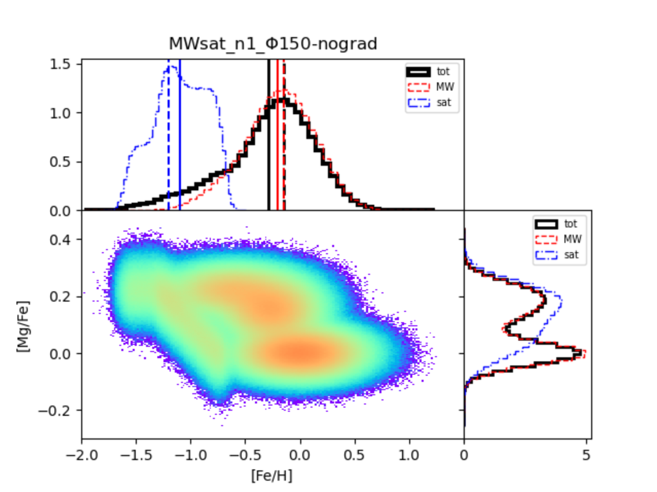
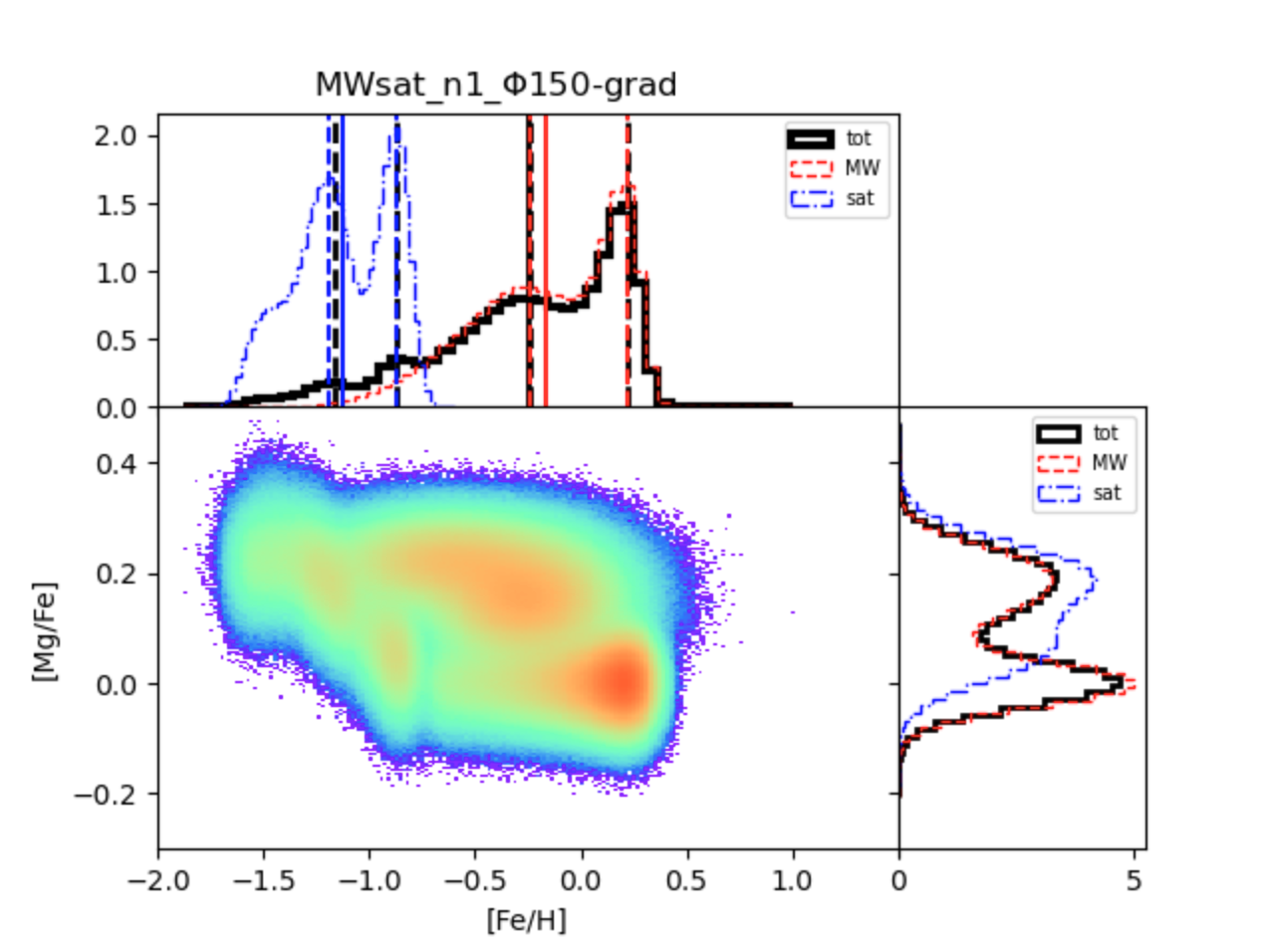
Figure 1: The $\rm{[Mg/Fe]}-\rm{[Fe/H]}$ space and its marginal distributions, for the case of a vertical metallicity gradient only (upper panel) and for the case of an additional radial metallicity gradient (lower panel).

Adding an initial radial metallicity gradient.

In this second case, we have explored the possibility that both the thin discs of the MW-type galaxy and the satellite initially show a negative radial metallicity gradient, which co-exist with the vertical gradients discussed before.

In the thin disc of the Milky Way, indeed, it is known that the inner regions have $\rm{[Fe/H]}\sim 0.3$, while the outer regions (beyond 10 kpc) have $\rm{[Fe/H]}\sim-0.7$ (e.g. Hayden et al., 2015). A metallicity gradient is currently absent in the thick disc (Cheng et al., 2012; Hayden et al., 2015), fact that could be due to its formation during a more turbulent phase, which would have led to an efficient mixing of metals (Haywood et al., 2013, 2015; Lehnert et al., 2014). The assignment of the radial metallicity gradient to the stellar particles is done on the basis of their initial ($t=0$) positions.
In particular, the metallicity of the thin disc particles of the MW-type galaxy is assigned as follows:

$$\rm{[Fe/H]}_{MW,thin}=\rm{[Fe/H]}_{MW,thin}^{max}-\frac{R}{R_{max,MWthin}}$$ (4)

where $R$ is the distance of the particle from the MW-type galaxy centre, projected in the disc plane, $\rm{[Fe/H]}_{MW,thin}^{max}$ is the maximum metallicity at the centre of the thin disc ($R=0$) which we have assigned equal to 0.3 dex and $R_{max,MWthin}$ is the maximum distance from the galaxy centre at which stellar particles of the thin disc of the MW-type galaxy are found. With $R_{max,MWthin}$ being equal to 50 kpc, this implies that Eqn. 4 can be rewritten as:

$$\rm{[Fe/H]}_{MW,thin}=\rm{[Fe/H]}_{MW,thin}^{max}-f_{MWthin}*R$$ (5)

with $f_{MWthin}=0.02$ dex/kpc. We caution the reader that the metallicity gradient of the Milky Way disc is known to be more complex than what we have used, with a steeper slope at few kpc from the Sun (Haywood et al 2023, A&A submitted, for a recent study). While the adopted values of the gradient can change the mean metallicities of stellar populations and the shapes of the MDFs, the bottom line of the results that we will present below do not change.

Similarly, for the thin disc of the satellite galaxy:

$$\rm{[Fe/H]}_{satthin}=\rm{[Fe/H]}_{satthin}^{max}-f_{satthin}*R$$ (6)

where $R$ is now the distance of a stellar particle of the satellite from the satellite centre, $\rm{[Fe/H]}_{sat,thin}^{max}$ is the maximum metallicity at the centre of the satellite thin disc (which we have assigned equal to -0.8 dex) and $f_{satthin}=0.05$ dex/kpc, in such a way that the satellite thin disc has a metallicity of -1.5 dex at its edge.

The bottom panel of Figure 1 shows the distribution of stars (accreted and in-situ) in the $\rm{[Mg/Fe]}-\rm{[Fe/H]}$ space when an initial radial metallicity gradient is added. The main trends are those observed already in the case of a vertical gradient only: the flatness of the [Mg/Fe] ratio for [Fe/H]$\lesssim-1.3$ dex, the appearance of a low-$\alpha$ sequence at higher metallicities, the redistribution of stars in an $\alpha$-enhanced thick disc and into a low-$\alpha$ thin disc counterpart. To these general features, the inclusion of a radial metallicity gradient has the effect to introduce a certain amount of complexity: the low-$\alpha$ thin disc sequence, as well as the low-$\alpha$ accreted sequence, are not anymore uniformly populated, but show prominent metal-rich peaks, which clearly appear in the total MDF, as well as in the MDF of the satellite and of the MW-type galaxy, taken separately. The $\alpha-$DFs, instead, stay the same, since in this second scenario no hypothesis on a $\alpha$-gradient with radius has been taken into account. In particular, in both cases (with or without a radial metallicity gradient) the $\alpha-$DF of the MW-type galaxies is bimodal, as found for stars in the MW disc (Haywood et al., 2018a).

In the following, we will refer to the two different initial conditions for the metallicity gradients with the suffix ”nograd”, to indicate the case where no radial metallicity gradient is initially present in the main and satellite discs, and to the suffix ”grad” to indicate the case where radial metallicity gradients are initially present. This suffix is added to the identificator of the simulation, as defined in the previous section. For example, the simulation named MWsat_n1_$\Phi$0_grad refers to a single 1:10 merger, where the satellite is initially on a planar prograde orbit, and where both the thin disc of the MW-type galaxy and of the satellite are initially characterised by a radial metallicity gradient.

3 Results

As far as the kinematics-related spaces are concerned, we confirm earlier results (Jean-Baptiste et al., 2017; Koppelman et al., 2020; Panithanpaisal et al., 2021; Amarante et al., 2022; Khoperskov et al., 2023c), i.e., that energy and angular momentum are not generally conserved quantities for such a significantly massive satellite, and this independently of the specific orbital inclination of the satellite galaxy relative to the main galaxy disc. Therefore, a single accretion event can redistribute stars over a large extent of the $E-L_{z}$ space and these stars are not smoothly redistributed in this space. They form clumps whose number and density depend on the number of passages the satellite has experienced around the MW-type galaxy before complete coalescence and on the mass loss it has experienced at each passage. The stars lost by the satellite in the early phases of its accretion onto the Galaxy tend to redistribute in the upper part of the $E-L_{z}$ space, that is at high energies. These stars also span a wide range of $L_{z}$ values. Hence, one accreted satellite gives rise to several overdensities in the $E-L_{z}$ space. On the other hand, stars which were in the disc of the main galaxy before the accretion are kinematically heated during the interaction, acquiring halo-like kinematics and thus contributing to the formation of a stellar halo together with the accreted stars (Zolotov et al., 2009; Purcell et al., 2010; Di Matteo et al., 2019, and references therein). As a consequence they redistribute in $E-L_{z}$ space in a region which partially overlaps with that of accreted stars.

3.1 Metallicity patterns in kinematic spaces

After the assignment of the metallicity to the star particles of the simulation, the first step we took has been to study the kinematics-related spaces with this additional information, in order to see where stars with different metallicity would redistribute and to check for a dependence on differences in the initial conditions for the metallicity gradients. We start by discussing the simulation with $\phi_{orb}=150^{\circ}$ to show the general trends in the kinematics-related spaces, then we will consider different volumes of the simulation to verify the feasibility of this kind of analysis with local observational data. Finally we will compare with the outcomes of the other simulations with different orbital parameters.

In Figure 2, we show the distributions in the $E-L_{z}$ space, since it is the most used in the literature among the different kinematics-related spaces, color-coded by the mean metallicity. The different columns of Figure 2 correspond to MW-type galaxy (first column), satellite (second one), and total (third one) stellar particles of the simulation. The first row shows the distributions in the $E-L_{z}$ space of all the star particles of the simulation for the ”nograd” case, resulting in both thin discs being more metal-rich than the thick ones on average. The second row shows the $E-L_{z}$ of the stars for the case of an additional initial radial metallicity gradient. Note that the scales of the color bars are different depending on which galaxy is considered, in order to make their specific metallicity patterns emerge in a more evident way. For the same purpose, the metallicity color bar does not cover the whole metallicity range of the metallicity distribution of the star particles of the galaxies of the simulation, but we have considered the percentiles of the distribution and restricted the range of the color bar to the $98\%$ of the metallicity distribution, as will be done in the rest of this analysis.

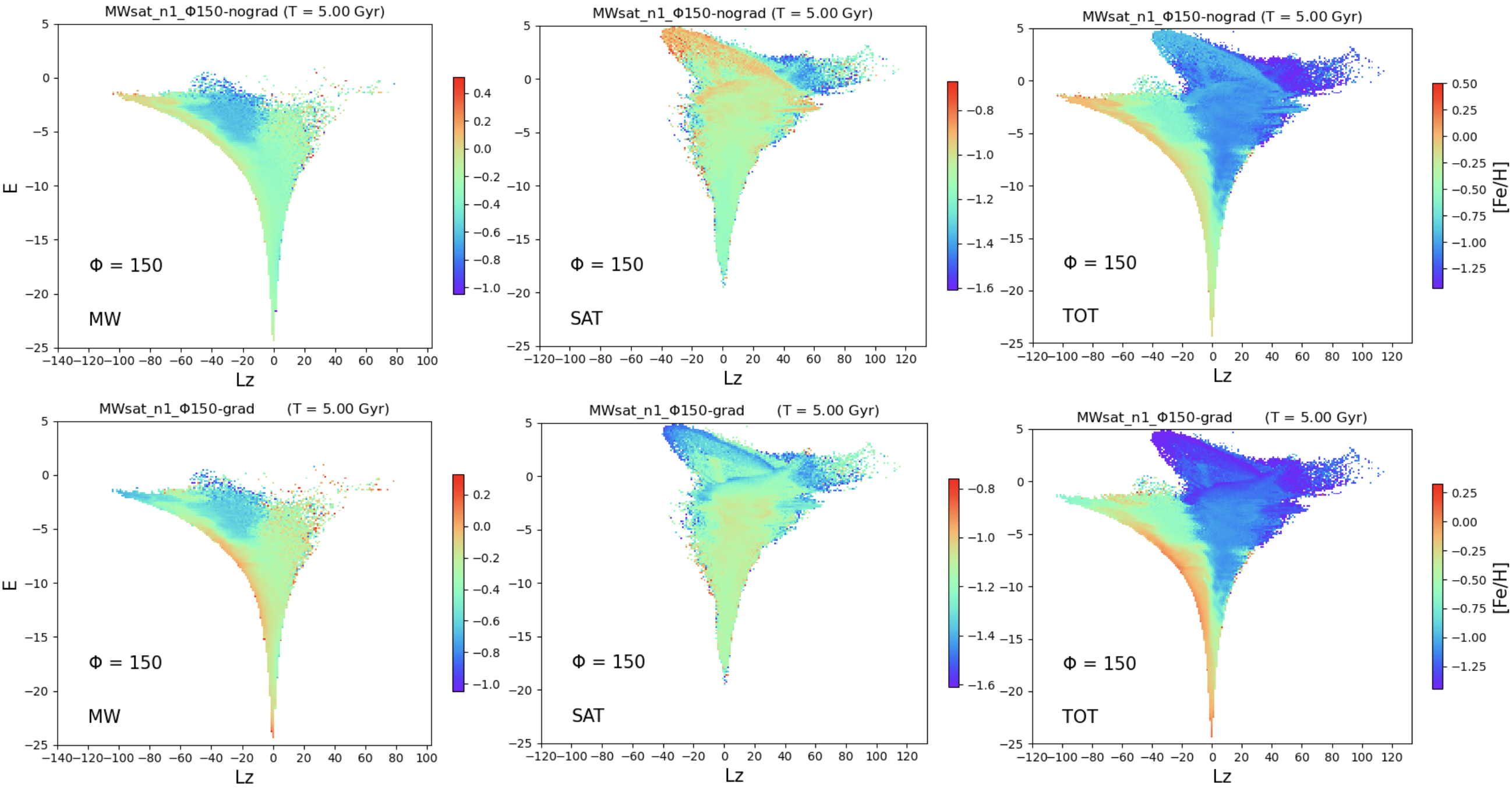
Figure 2: $E-L_{z}$ space of in-situ (first column), satellite (second column) and total (third column) star particles in the simulation, color-coded for their mean metallicity. The first and second rows show the $E-L_{z}$ space for the case of initial vertical gradient only and for an additional initial radial metallicity gradient, respectively. Note that the scales of the color bars are different depending on which galaxy is considered, in order to make their specific metallicity patterns emerge in a more evident way. We also recall that in these plots stars on prograde orbits (which rotate as the disc) have negative $L_{z}$, while stars on retrograde orbits have positive $L_{z}$.

As far as the in-situ star distribution in the $E-L_{z}$ space is concerned (top left plot), we can observe where the different disc components of the MW-type galaxy, characterised by different mean metallicity, dominates in the $E-L_{z}$ space. We can see that the most metal-rich stars (in orange-red) redistribute in the region of prograde circular orbits of the thin disc, while the most metal-poor stars (violet-blue) are mainly found in the $E-L_{z}$ region dominated by the thick disc.

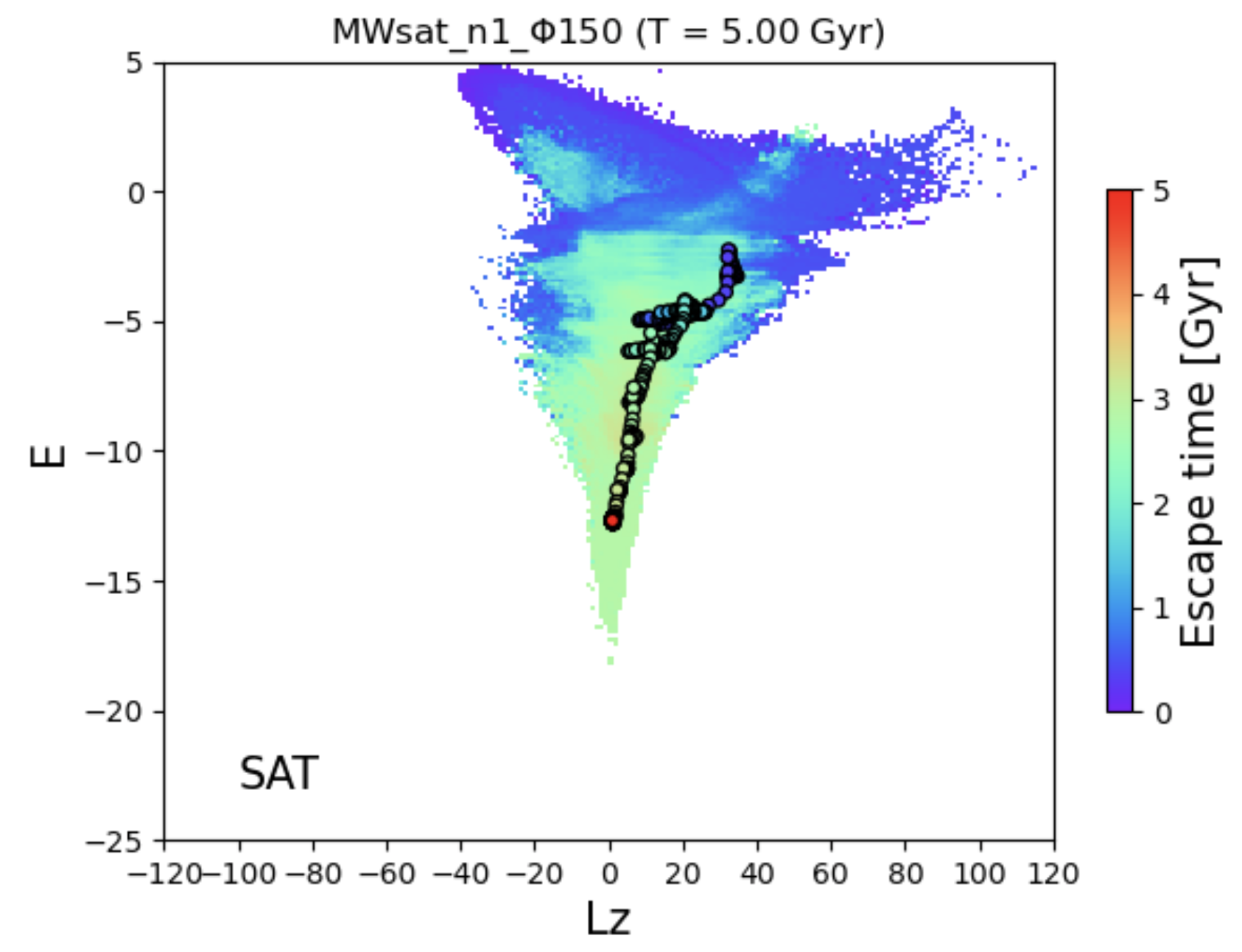
Figure 3: Final distribution of the satellite stars in the $E-L_{z}$ space as in the middle column of Figure 2, but color-coded by their escape time from the satellite potential. The dots represent the mean values of energy and z-component of the angular momentum of bound satellite stars, defined by being at less than 15 kpc from its barycentre. There are five hundreds dots (one for each snapshot of the simulation) and they are color-coded with the same color-bar scale but for the time of the simulation (every 10 Myr to cover the 5 Gyr time interval).

Regarding the satellite stars distribution (top middle plot), instead, we can notice that there is a region in the upper part of the $E-L_{z}$ space where the mean metallicity is higher on average. This region is characterised by very high values of energy, thus being the region populated by the first stars that escape from the satellite during its interaction with the main galaxy, being lost in the MW-type galaxy potential (Figure 3). These stars are those in the outskirts of the satellite thin disc, indeed - since they are at larger (radial) distances from the satellite baricenter - they are less bound to its potential and thus more inclined to leave it. In the case we are considering now of no radial gradient in the thin disc, but only a negative vertical metallicity gradient, we have that the thin disc stars are the most metal-rich, hence explaining the mean metallicity pattern of the satellite distribution in the $E-L_{z}$ space.

Thus, the existence of an initial metallicity gradient inside the satellite has a consequence in the $E-L_{z}$ space: different regions show different mean metallicity. We will check in the following Section 3.2 how this fact also reflects in the metallicity distribution functions of the different regions, in order to see if in addition to change in the mean value of the distribution, also its shape changes. Finally, as long as the total star distribution is concerned (top right plot), we can observe a strong metallicity gradient in the $E-L_{z}$ space, which reflects the regions where the more metal-rich in-situ stars dominate on more prograde orbits and lower energy values and the ones where instead most of the more metal-poor satellite stars lie on more retrograde orbits and higher energy values. In addition to the fact that on average in-situ stars are more metal-rich than satellite ones, we can still observe that inside the distribution of these two galaxies there are metallicity gradients, as described above.

In order to verify whether these results would be dependent on differences in the initial conditions for the metallicity gradients, we have also studied the case of an additional radial negative gradient in the thin discs of both the satellite and the MW-type galaxy, thus being the outskirts of the discs more metal-poor than the inner parts. We report the corresponding results in the second row of Figure 2: the MW-type galaxy distribution (left plot) overall resembles the one seen previously for the case of vertical metallicity gradient only. However, we can notice the effect of having introduced a negative radial gradient too: the region of the $E-L_{z}$ space populated by the thin disc (towards the edge of the $E-L_{z}$ distribution, for negative values of $L_{z}$) is not anymore homogeneously colored as it was on the case of a vertical metallicity gradient only, but exhibits a gradient. We can see that the upper regions are more metal-poor than in the previous case. These regions at high energies are, indeed, populated by stars which initially are the less gravitationally bound (i.e. high energies and large distances from the main galaxy center). On the other hand, the low energy regions are more metal-rich than before, because the populations initially more gravitationally bound (and more metal-rich) are also closer to the galaxy centers. As far as the satellite distribution is concerned (middle plot), we can again observe the consequence of the choice made for the initial metallicity gradient: the upper region that was before populated by the most metal-rich stars, is now on the contrary populated by the most metal-poor stars. This is clearly a consequence of assigning a radial metallicity gradient to satellite disc stars. Finally, regarding the total distribution (right plot), we can observe an overall metallicity gradient again, which is even stronger than before (see Section 3.4), and still we can see the gradients inside the two galaxies.

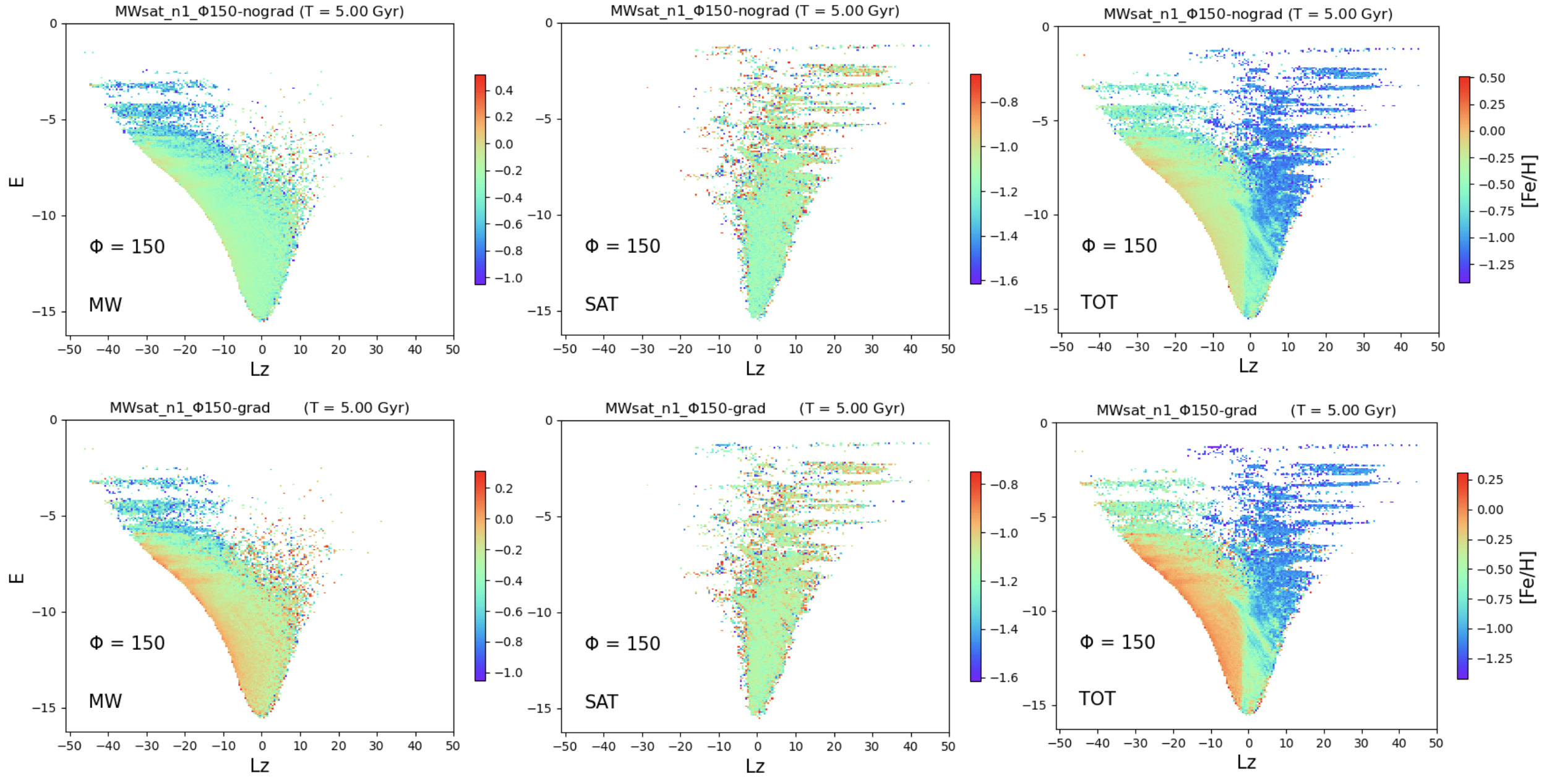
Figure 4: $E-L_{z}$ space of in-situ (first column), satellite (second column) and total (third column) star particles in the simulation, color-coded for their mean metallicity, when the analysis is restricted to a solar-like volume. The first row shows the $E-L_{z}$ space for the case of an initial vertical metallicity gradient only. Likewise, the second row, but for the case of an initial additional radial metallicity gradient. Note that the scales of the color bars are different depending on which galaxy is considered, in order to make their specific metallicity patterns emerge in a more evident way. We also recall that in these plots stars on prograde orbits (which rotate as the disc) have negative $L_{z}$, while stars on retrograde orbits have positive $L_{z}$.

3.1.1 Solar-like volume

Once the previous results for the total distributions of star particles in the $E-L_{z}$ space are obtained, we are interested in understanding what it is actually possible to obtain with the data we have in a limited volume observed. Thus in order to check the feasibility of detecting accreted structures in this space in local volumes, we restrict our analysis to a “solar-vicinity” or a “solar-like volume”. It is defined as a spherical volume centered at 8 kpc from the MW-type galaxy center and has a radius of 5 kpc, which is the typical size around the Sun for which we currently have accurate enough parallaxes, proper motions and line-of-sight velocities. In order to take into account the fact that accreted stars do not necessarily redistribute uniformly, we have considered several different volumes homogeneously distributed in the azimuth position of the center: $\phi_{\odot}=0^{\circ},90^{\circ},180^{\circ},270^{\circ}$ (in cylindrical coordinates). In the following analysis, we will show the results for the first solar volume (with $\phi_{\odot}=0^{\circ}$), which are also valid for all the other volumes examined. Figure 4 shows the final distributions in the $E-L_{z}$ space when the solar-like volume is considered.

We can see in the right-most panels of Figure 4, that the same overall trend observed for the whole volume are found: a metal-poor population with retrograde or null $L_{z}$, and a more metal-rich one as the orbits become more prograde (negative $L_{z}$), for both the metallicity gradient cases. Furthermore, it is interesting to notice how a retrograde single-merger event can produce a Sequoia-like debris, which corresponds to the outer parts of its GSE-like progenitor. However, when the analysis is restricted to 5 kpc around the Sun, we cannot capture anymore the very metal-rich (metal-poor) satellite stars found at very high energies: see, for example, orange (blue) color in the middle panel of the top (bottom) row of Figure 2. This implies that the MDF of the GSE may still exhibit biases, particularly in the absence of observations for the most metal-rich (metal-poor) stars. This limitation could potentially be addressed more comprehensively with upcoming surveys such as SDSSV/4MOST or, more promisingly, with MOONS.

3.1.2 Exploring different orbital inclinations

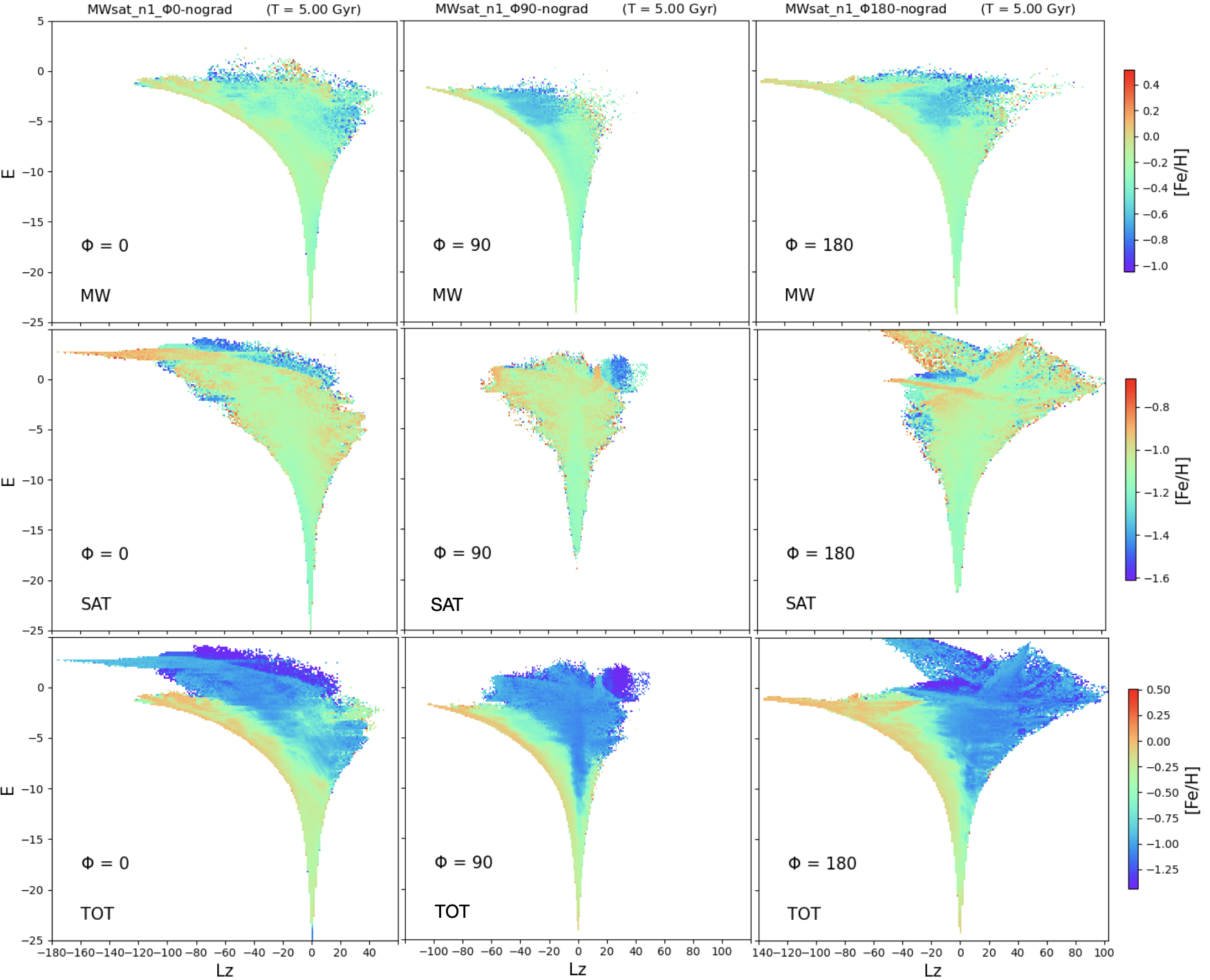
Figure 5: $E-L_{z}$ spaces of the in-situ (first row), satellite (second row) and total (third row) star particles in the simulation, color-coded for their mean metallicity, for the case of an initial vertical metallicity gradient only. Each column shows a simulation with a different value of the initial inclination of the satellite orbital plane: $\phi_{orb}=0^{\circ},90^{\circ},180^{\circ}$.

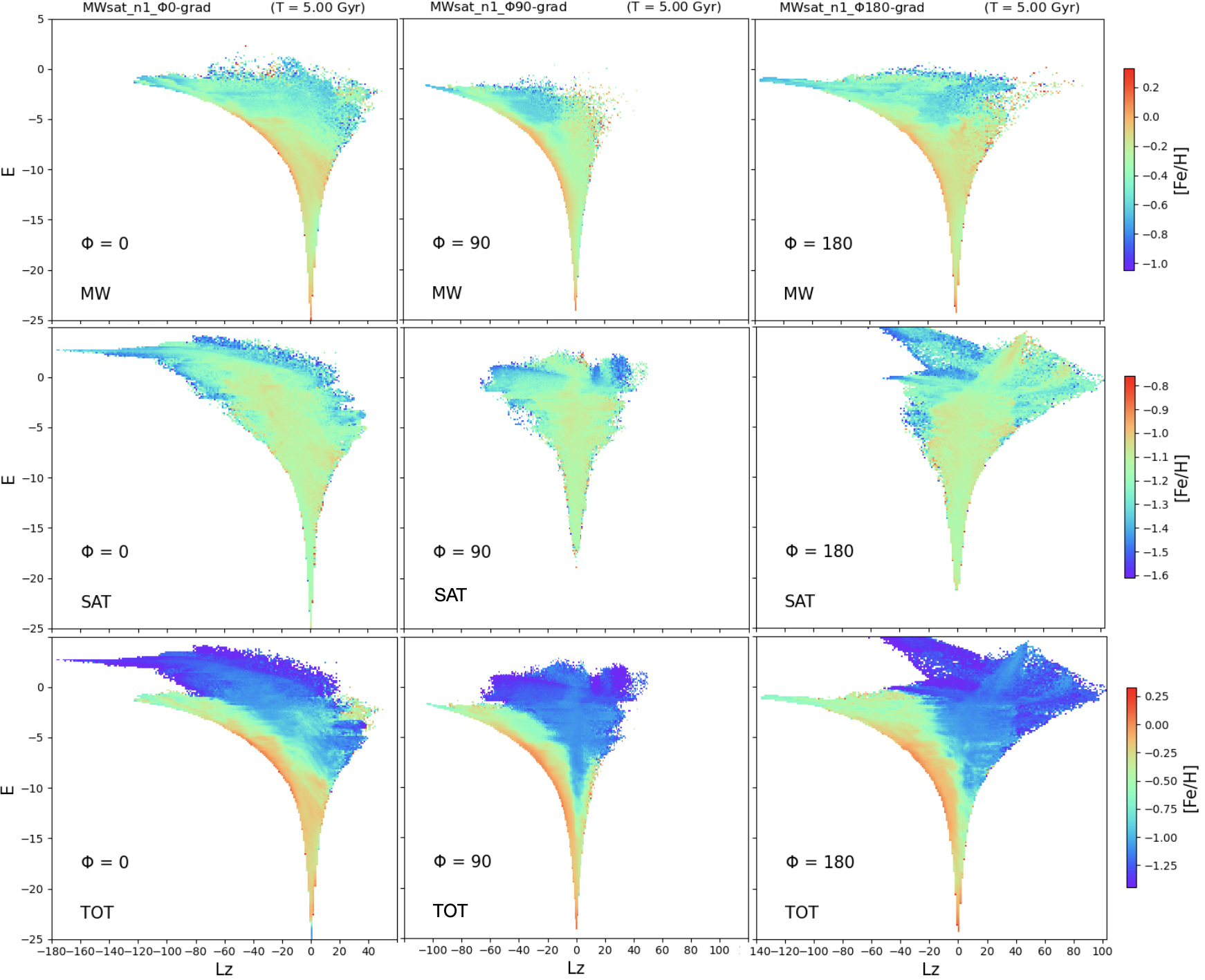
Figure 6: Same as Figure 5, but for the case of an initial additional radial metallicity gradient.

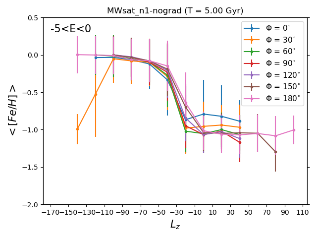
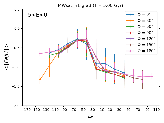
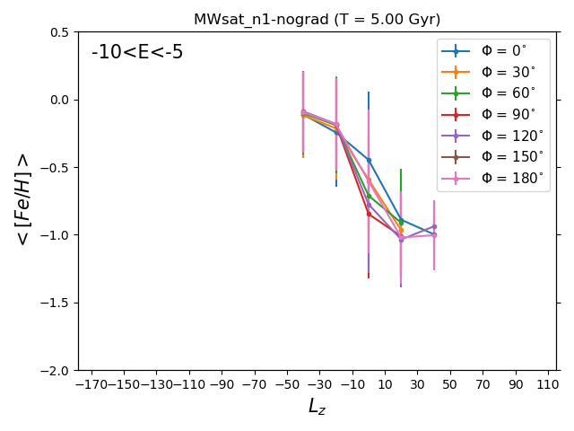
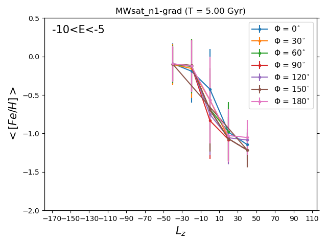
Figure 7: Mean metallicity and standard deviation as a function of the angular momentum interval of the $E-L_{z}$ space (in every column of Figures 8, 12) for all the simulations with $\Phi=0^{\circ},30^{\circ},60^{\circ},90^{\circ},120^{\circ},150^{\circ},180^{\circ}$, in the energy range $-5<E<0$. Left panel shows the case with the initial vertical metallicity gradient only, while the right panel the one with the additional radial metallicity gradient.

In order to check for the dependence of our results on the satellite orbital parameters, we have analysed the star distributions in all the previous spaces (color-coded by the mean metallicity) for all the other simulations with different initial inclination of the satellite orbital plane with respect to the MW-type galaxy, $\phi_{orb}=0^{\circ},30^{\circ},60^{\circ},90^{\circ},120^{\circ},150^{\circ},180^{\circ}$. For a seek of synthesis, in the following we only report the results for the $E-L_{z}$ space for $\phi_{orb}=0^{\circ},90^{\circ},180^{\circ}$. In Figures 5-6, we show the final distributions in the $E-L_{z}$ space color-coded by the mean metallicity for the total volume of the simulation, for the in-situ (first column), satellite (second column) and total (third column) star particles.

Figure 5 shows the distributions in the case of an initial vertical metallicity gradient only. The in-situ distributions are all very similar (note the different range on the $x-$axis). The satellite distributions, instead, show a dependence on the orbital parameter $\phi_{orb}$, with: (i) more metal-poor stars on prograde orbits (negative values of $L_{z}$) at high energies for initial prograde orbits of the satellite, and (ii) more on retrograde orbits at high energies for initial retrograde orbits of the satellite. In any case, the most metal-rich stars are those of the thin disc, lost early and at high values of energy. These two features can be observed in the total distribution, which shows different regions dominated by metal-poor stars, depending on the initial satellite orbital properties.

In Figure 6, we show the same distributions for the case of an initial additional radial metallicity gradient. The in-situ distributions are all very similar (note the different range on the $x-$axis), this time showing the radial metallicity gradient in the region of the circular prograde orbits (thin disc). As long as the satellite distributions are concerned, on the contrary with respect with before, the most metal-poor stars are the ones of the thin disc, lost at low values of time and high values of energy. The distributions of satellite stars still show a dependence on the orbital parameter $\phi_{orb}$, with more metal-poor stars on prograde orbits (negative values of $L_{z}$) at high energies for initial prograde orbits of the satellite and more on retrograde orbits at high energies for initial retrograde orbits of the satellite. Again, this can be appreciated in the total distribution, which then shows different regions dominated by metal-poor stars, depending on the initial satellite orbital properties. This dependence could be useful to characterise the orbital parameters of the accretion events experienced by the Milky Way. However this can be challenging if the analysis is restricted to a volume of few kpc in radius around the Sun (as it is the case of many spectroscopic surveys). When we restrict the analysis to the solar-like volume, indeed, the final distribution in the $E-L_{z}$ space become all very similar one to each other, losing the dependence of the metallicity pattern on the $\phi_{orb}$ parameter, since the difference in the final distribution considering the whole volume are due to satellite stars deposited at high energy values, which do not reach the solar vicinity.

As mentioned above, the mean metallicity throughout the $E-L_{z}$ space for bound regions does not depend strongly on the orbital parameters of the accretion event. More quantitatively, we show in the upper row of Figure 7 the mean metallicity (and standard deviation) in the energy interval $-5<E<0$ as a function of the angular momentum for all the possible initial values of the inclination of the satellite orbital plane (different colors) and for both the ”nograd” (left panels) and the ”grad” case (right). We can see a dependence on the initial conditions assumed for the metallicity distribution of the satellite. In fact, both the left and right panels show a ”knee” at approximately null angular momentum and then a plateau at low metallicity at more retrograde $L_{z}$ values (more positive). However, the ”nograd” case also features a plateau at high metallicity and at prograde angular momentum values (negative $L_{z}$), whereas the ”grad” case shows a decreasing mean metallicity value the more prograde the orbit. In the lower row of Figure 7, we also show the same plots in the energy interval $-10<E<-5$ for a comparison.

3.2 MDF in different regions of the $E-L_{z}$ space

After discussing the variation of the mean metallicity across the $E-L_{z}$ space, the following step is to analyse the variation of the metallicity distribution functions. The interest into looking at the MDF is due to the fact that all previous plots show the average metallicity in a given region of the $E-L_{z}$ plane, while the MDF can provide more insight on the population(s) which contribute to a given average value. As before, at the beginning, we show the results for the simulation with the initial inclination of the satellite orbital plane with respect to the MW-type galaxy disc, $\phi_{orb}$, equal to $150^{\circ}$. The results concerning the simulations with direct, polar and retrograde orbits ($\phi_{orb}=0^{\circ},90^{\circ},180^{\circ}$) are reported in the Appendix A.

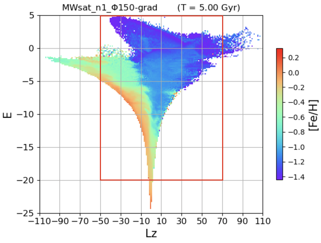
Figure 8: Total star distribution in the $E-L_{z}$ space for the case of an initial vertical metallicity gradient only (upper panel) and of an initial additional radial metallicity gradient (lower panel), color-coded by the mean metallicity. The grid over-imposed shows the splitting of the space used to analyse the metallicity distribution functions in different regions.

In order to analyse the MDFs in different regions of the $E-L_{z}$ space, we have divided this space in rectangles $20\times 10^{2}$ kpc km/s wide in angular momentum and $5\times 10^{4}$ km² s^-2 high in energy, as to reproduce an average dimension of the substructures found so far in the $E-L_{z}$ space. We have then obtained eleven bins in the x-axis, and six bins in the y-axis, as shown in Figure 8. In Figure 9 we show the resulting MDFs for different regions of the $E-L_{z}$ space contained in the red rectangle of Figure 8. In this way, different rows show the MDFs for a fixed value of energy (increasing in the bottom-up direction), while different columns show the MDFs for a fixed value of angular momentum (increasing in the left-right direction). Every plot then shows the MDF considering all the stars in the region (in black), the MDF of the MW-type stars only (in red) and the MDF for the satellite stars only (in blue), all normalised in order to compare means, peaks and shapes. The solid lines show the mean of the distribution, while the dotted ones show its peak(s). The values of the number of stars in the different $E-L_{z}$ regions, as well as the mean metallicities, and peaks of the MDFs, for the two cases (”nograd” and ”grad”) explored in this paper, are reported in Tables 5, 6 and 7.

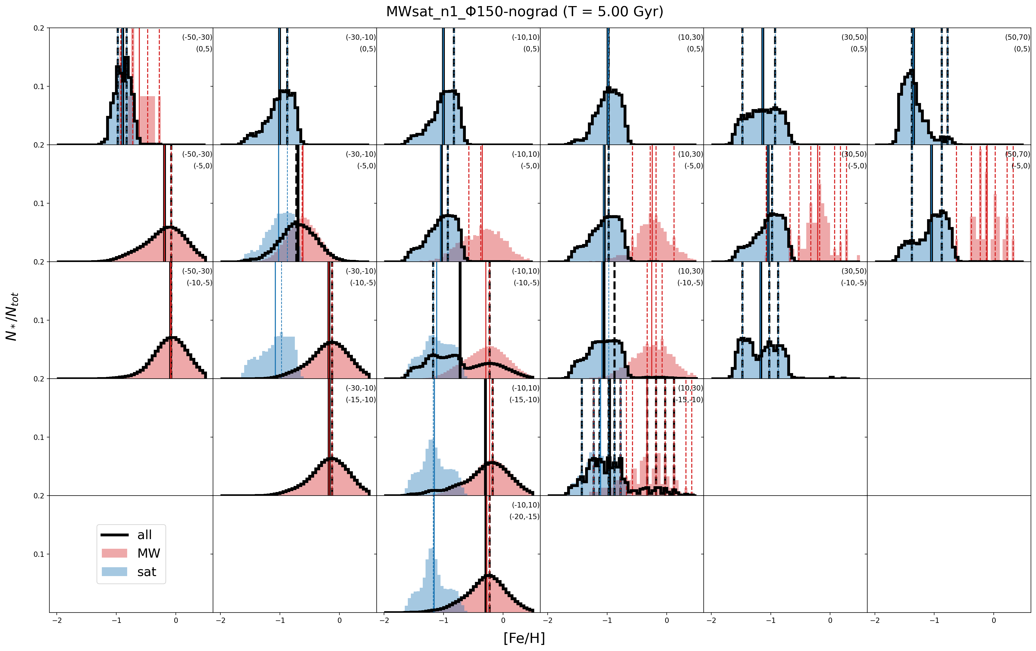
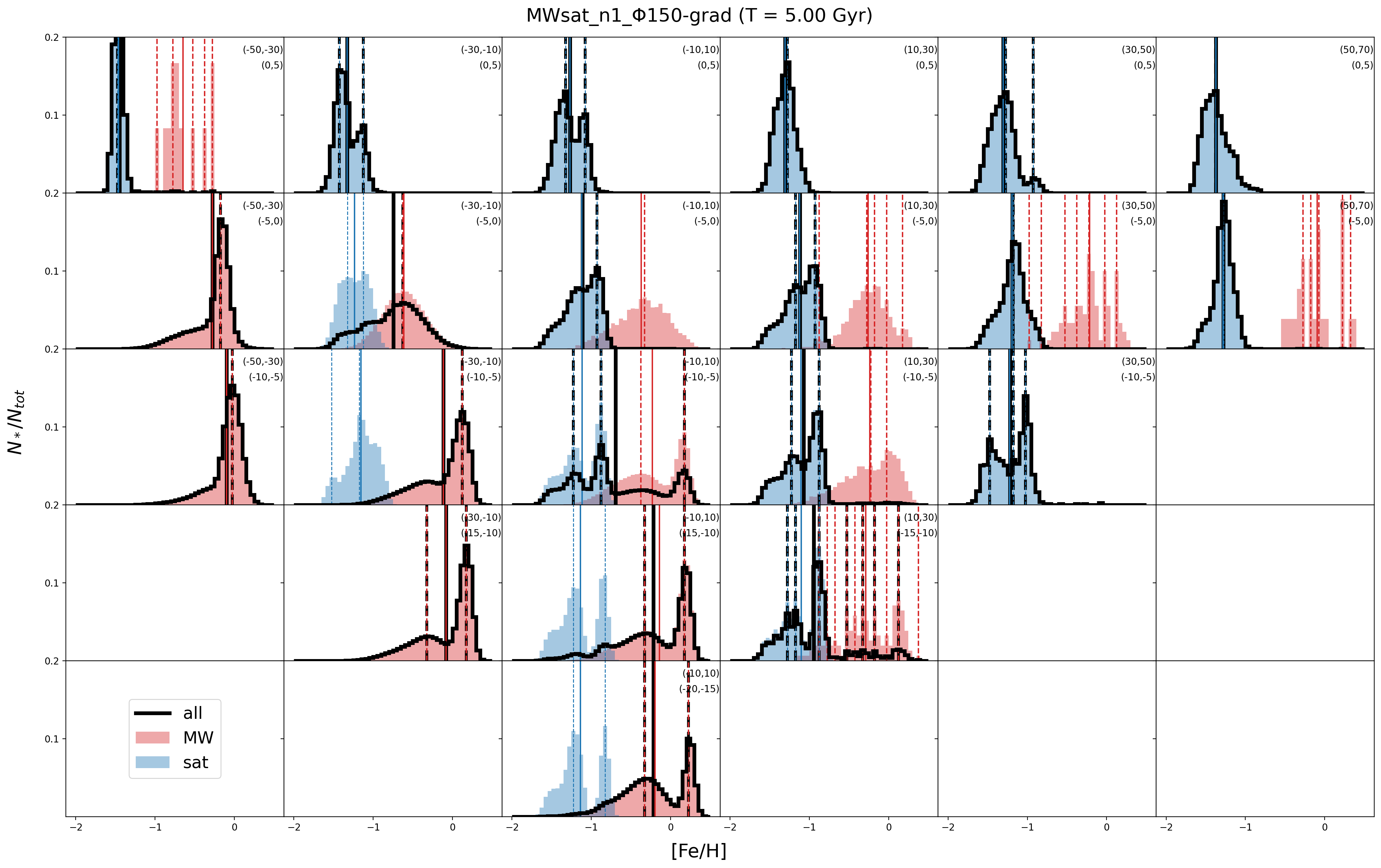
Figure 9: MDFs of different regions of the $E-L_{z}$, for the ”nograd” case (top panel) and for the ”grad” one (bottom panel). The red, blue and black histograms show the MW-type galaxy, satellite and total MDF, respectively, all normalised. The solid lines show the mean of the distribution, while the dotted ones its peak(s). Energy intervals row by row (top to bottom): i) 0 ¡ E ¡ 5, ii) -5 ¡ E ¡ 0, iii) -10 ¡ E ¡ -5, iv) -15 ¡ E ¡ -10, v) -20 ¡ E ¡ -15. Angular momentum intervals column by column (left to right): i) -50 ¡ $L_{z}$ ¡ -30, ii) -30 ¡ $L_{z}$ ¡ -10, iii) -10 ¡ $L_{z}$ ¡ 10, iv) 10 ¡ $L_{z}$ ¡ 30, v) 30 ¡ $L_{z}$ ¡ 50, vi) 50 ¡ $L_{z}$ ¡ 70.

We start from the case of a vertical metallicity gradient only. The $E-L_{z}$ space has been divided as described above and as shown in the top panel of Figure 8. Starting from the bottom row of Figure 9, i.e. the lowest energy interval considered ($-10\leq L_{z}\leq 10,-20\leq E\leq-15$), the global MDF in black of both accreted and in-situ stars almost coincides with that of in-situ stars only, since they dominate this region (see Figure 1). The central rectangle of the following row ($-15\leq E\leq-10$) is still dominated by in-situ stars, but now the total MDF shows a bump at low metallicity ($\rm{[Fe/H]}\sim-1.2$) due to satellite stars. So far, satellite MDFs are all very similar one to each other, resembling the total satellite MDF (see Figure 1): single-peaked distribution (at $\rm{[Fe/H]}\sim-1.2$), with a bump at higher metallicities. The following row ($-10\leq E\leq-5$) shows, instead, some differences. The satellite MDF starts to peak at higher metallicities (at $\rm{[Fe/H]}\sim-1$) in the central region with $L_{z}\sim 0$, due to the fact that a larger fraction of satellite metal-rich stars are found at higher energies as they escape the satellite at earlier times. Moreover, we observe a broader distribution in the region with $-10\leq L_{z}\leq 10$ and a region in which the MDF is double-peaked ($10\leq L_{z}\leq 30$), even if the initial total MDF of the satellite was not. We also see that the total MDF in regions with stars on more retrograde orbits has significant contributions from the satellite stars at low metallicities. As a consequence, its mean is shifted towards lower metallicities while moving towards more retrograde orbits (more positive values of $L_{z}$), but also towards higher energies, where satellite stars represent a higher fraction with respect to the total (see Table 5). We can observe all these features in the least bound row ($-5\leq E\leq 0$), where the distributions are broader and peaked at lower metallicities as we move towards more retrograde star orbits (positive $L_{z}$). In particular the right-most plot of the figure, which contains stars with highest energies and most retrograde orbits, is the one where the MDF peaks at the lowest metallicities, i.e. at $\rm{[Fe/H]}\sim-1.5$. For completeness, we also report the unbound energy interval $0<E<5$. We can appreciate also in this region the same trend, namely that the mean of the total MDF decreases for more retrograde orbits.

$\downarrow E;L_{z}\rightarrow$	$(-110,-90)$	$(-90,-70)$	$(-70,-50)$	$(-50,-30)$	$(-30,-10)$	$(-10,10)$	$(10,30)$	$(30,50)$	$(50,70)$	$(70,90)$	$(90,110)$
(0,5)	-	-	-	0.99	1.00	1.00	1.00	1.00	1.00	1.00	1.00
(-5,0)	-	-	-	-	0.21	0.99	1.00	1.00	1.00	0.99	-
(-10,-5)	-	-	-	-	0.00	0.53	0.96	0.99	-	-	-
(-15,-10)	-	-	-	-	-	0.08	0.8	-	-	-	-
(-20,-15)	-	-	-	-	-	0.02	-	-	-	-	-
(-25,-20)	-	-	-	-	-	-	-	-	-	-	-

Table 5: Fraction of satellite stars with respect to the total in every cell of Figure 8.

We now discuss the results for the case of an additional initial radial metallicity gradient, both in the satellite and in the MW-type galaxy. We recall that the introduction of the radial gradient makes the MDFs of both the MW-type galaxy and the satellite double-peaked (see Figure 1). The highest peak is due to the thin disc component and the second to the intermediate and thick disc components together (see middle row of Figure 10, where we show the MDF of the various disc components in different colours.) The in-situ MDF peaks are at $\rm{[Fe/H]}\sim 0.2$ and at $\rm{[Fe/H]}\sim-0.2$, while the satellite MDFs are at $\rm{[Fe/H]}\sim-0.9$ and at $\rm{[Fe/H]}\sim-1.2$. We are then interested to check if we recover these features in the MDF restricted to different regions of the $E-L_{z}$ space. We proceed in the same way as the previous case, so the $E-L_{z}$ space has been divided as before and as shown in the lower panel of Figure 8. In the bottom row of Figure 9, we show the MDFs in the $E-L_{z}$ space with $E\leq-15$. We can see that the MDF of the single galaxies, the MW-type galaxy (in red) and the satellite (in blue), are usually quite representative of the total initial ones, being bimodal and peaked at the initial positions in metallicities. Nevertheless, considering higher energy intervals ($-15\leq E\leq-10$ and $-10\leq E\leq-5$), the total MDF (in black) already starts to change, reflecting the increasing relative importance of the satellite contribution, thus beginning to show bumps at lower metallicities and means more shifted towards lower metallicities too. This trend is hence independent of the choice for the initial conditions for the metallicity gradient, but is mostly due to the fact that regions of higher energies and more retrograde angular momentum are more dominated by the satellite stars (see Table 5), which are on average more metal-poor. In the regions with the highest energies (bound and not, $-5\leq E\leq 0$ and $0\leq E\leq 5$), we can see that the satellite MDFs change a lot in shape and mean, becoming broader, losing the bimodality and being on average at lower metallicities. Once again the total MDF coincides always more with the satellite one, moving towards higher energies and more retrograde orbits, thus changing a lot in mean towards lower metallicities.

We can then conclude that, independently of the initial choice for the metallicity gradient of the satellite, its MDFs in different regions of the $E-L_{z}$ space can be significantly different one from each other in shape, mean and peak values, even if they are all resulting from the same accretion event. Therefore different regions of the $E-L_{z}$ space showing different kinematic and MDFs can actually be associated to the same single original accreted satellite, making the $E-L_{z}$ very hard to interpret. Nevertheless, we have found trends in the MDFs varying energy and angular momentum values. In particular, we have shown that the mean and the peak(s) of the global MDF of both accreted and in-situ stars move towards lower metallicities for higher values of energy and angular momentum (i.e. for more retrograde orbits). This is a consequence of the increasing importance of the more metal-poor satellite contribution in stellar density.

3.2.1 Global versus local MDFs

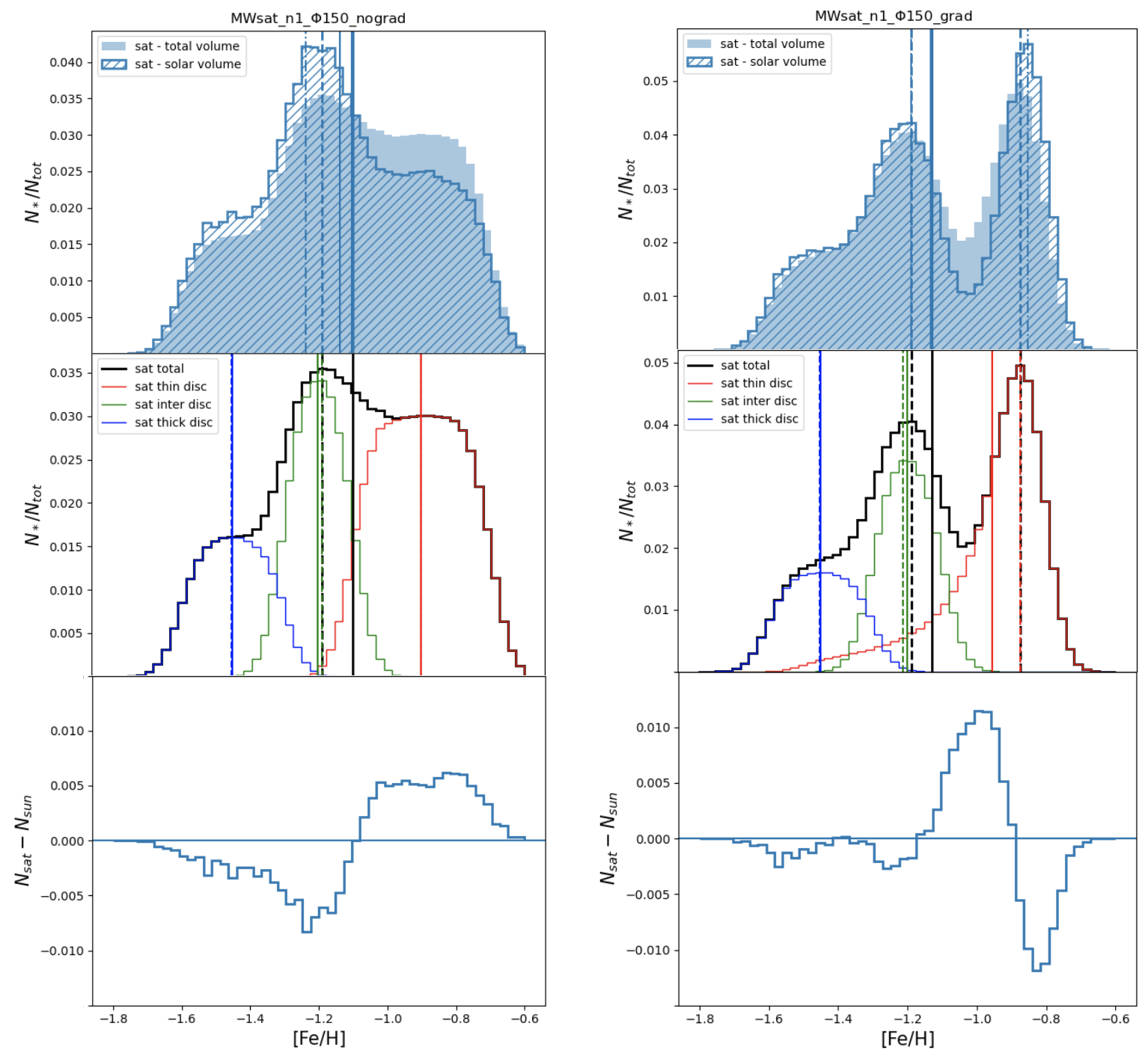
Figure 10: Top panels: MDF of the satellite stars (in filled blue) and the same MDF restricted to the satellite stars that reach the solar-like volume within the end of the simulation (in patterned blue). The solid lines are the mean of the distributions (broader for the total distribution, thinner for the solar one). The dashed (dot-dashed) lines are the peak(s) of the total (solar) distribution. Middle panels: Satellite MDF divided in disc components. Bottom panel: Difference between the two distributions in the top panel, i.e. total distribution minus solar-like restricted one. Left column shows the case with the vertical metallicity gradient only, while the right column the one with the additional radial metallicity gradient.

So far, we have shown MDFs estimated over the whole galactic extent, in the ideal case – as it is in a simulation – where all stars (or stellar particles) in the galaxy can be observed. In reality, spectroscopic surveys provide chemical abundances over a limited volume around the Sun. It is thus interesting to understand to what extent a ”local” MDF can be representative of the global one. In particular, if we were able to select a pure (that is with null or very limited pollution of in-situ stars) accreted sample of stars at few kpc from the Sun, to what extent its MDF would be representative of that of the whole satellite?

We recall that we defined the “solar-vicinity”, as a spherical volume centered at 8 kpc from the MW-type galaxy center and with a radius of 5 kpc. The top panels Figure 10 show the MDF of all satellite stars (in filled blue) and its local counterpart, where only the contribution of stars which at the end of the simulation are found in a solar-like volume are shown (in patterned blue). Both the cases with and without an initial radial metallicity gradient in the satellite are shown (right and left panels respectively). We can notice that in both cases the global shape of the MDF is conserved, as also the metallicity range featured. The bottom panels show the difference between the two distributions. We can see that for the ”nograd” case, there is an under-representation of high metallicity stars (i.e. stars with $\rm{[Fe/H]}\geq-1.1$), while for the ”grad” case there is deeper drop at $\rm{[Fe/H]}\sim-1.0$. By a comparison with the middle row plots, which show the satellite total MDFs, along with the MDFs of the single disc components (thick, intermediate and thin ones), we can associate the under-representation to missing thin disc stars, i.e. to stars initially in the outskirts of the satellite which are lost in the early phases of the accretion, and that are deposited at too high energies to be sampled at the solar vicinity. Depending on the metallicity that these stars initially have, this will give rise to an under-representation of these metallicities in local MDFs.

3.3 Reconstructing a possible (but wrong) accretion history from kinematic spaces and MDFs

The results discussed in the previous section can lead to reconstruct accretion histories which may look realistic, but which are in fact very far from the ”true” one. An example of the difficulty of using these spaces to reconstruct the merger tree of a MW-type galaxy is given below.
Suppose we have a dataset of halo stars, distributed over an extended range of energies and angular momenta. We might be led to interpret different regions of this space as being dominated by stars of different origins, and to infer the properties of the galaxies in which these stars formed by studying the characteristics of their MDFs. For example, by making use of a mass-metallicity relation as given by (Kirby et al., 2013)

$$<\rm{[Fe/H]}>=(-1.69\pm 0.04)+(0.30\pm 0.02)\log\left(\frac{M_{*}}{10^{6}M_{\odot}}\right).$$ (7)

we may in principle reconstruct the stellar mass of the progenitor galaxies, given the mean metallicity of stars in a given $E-L_{z}$ region. If we apply this reasoning to our simulations, we would get the following:

• Unbound stars ($0<E<5$) found in the ”nograd” simulation (upper panel of Figure 8) are dominated at null angular momentum ($-10<L_{z}<10$) by stars of a galaxy whose stellar mass was $\sim 10^{8.4}M_{\odot}$, since the mean metallicity of stars in this region is $<\rm{[Fe/H]}>\sim-1.0$, while stars of the same energy but more retrograde angular momenta ($50<L_{z}<70$) would be associated to a satellite galaxy of stellar mass equal to $10^{7}M_{\odot}$, given that the mean stellar metallicity in this region is $<\rm{[Fe/H]}>\sim-1.4$.

• At lower energies ($-10<E<-5$), the problem would persist. In particular, in the region around null angular momentum ($-10<L_{z}<10$), the mean metallicity being $<\rm{[Fe/H]}>\sim-0.7$, this may be interpreted as signature of a massive accretion $M_{*}\sim 10^{9.4}M_{\odot}$.

• Similar conclusions would hold for the ”grad” case, where, depending on the region we look at, we may end with finding traces of low-mass accretions ($M_{*}\sim 10^{7.4}M_{\odot}$ at $-5<E<0$ and $50<L_{z}<70$, corresponding to a mean $<\rm{[Fe/H]}>\sim-1.3$) and also more massive ones ($M_{*}\sim 10^{8.4}M_{\odot}$ at $-10<E<-5$ and $10<L_{z}<30$, corresponding to a mean $<\rm{[Fe/H]}>\sim-1.0$).

An even more complex situation would arise if we try to interpret the multiple peaks present in the MDFs of some specific regions of the $E-L_{z}$ space, as due to distinct accretion events.

Regardless of the details of the average metallicity values and thus masses of the progenitors, the common feature of this type of analysis is to overestimate the number of accretions and underestimate the associated masses.

$\downarrow E;L_{z}\rightarrow$	$(-50,-30)$	$(-30,-10)$	$(-10,10)$	$(10,30)$	$(30,50)$	$(50,70)$
(0,5)	-0.90	-1.01	-1.01	-0.99	-1.13	-1.36
(-5,0)	-0.19	-0.69	-1.04	-1.05	-1.04	-1.05
(-10,-5)	-0.09	-0.18	-0.72	-1.06	-1.16	-
(-15,-10)	-	-0.17	-0.29	-0.96	-	-
(-20,-15)	-	-	-0.29	-	-	-

Table 6: For every cell of the top panel of Figure 8 (”nograd” case), we report the mean value of the metallicity distribution of all the stars.

$\downarrow E;L_{z}\rightarrow$	$(-50,-30)$	$(-30,-10)$	$(-10,10)$	$(10,30)$	$(30,50)$	$(50,70)$
(0,5)	-1.45	-1.33	-1.27	-1.31	-1.31	-1.38
(-5,0)	-0.28	-0.74	-1.11	-1.12	-1.19	-1.28
(-10,-5)	-0.09	-0.12	-0.69	-1.07	-1.22	-
(-15,-10)	-	-0.08	-0.22	-0.95	-	-
(-20,-15)	-	-	-0.21	-	-	-

Table 7: For every cell of the bottom panel of Figure 8 (”grad” case), we report the mean value of the metallicity distribution of all the stars.

3.4 Metallicity gradient in the satellite vs. in the $E-L_{z}$ space

Once it is established that analysing separately the metallicity distribution of limited regions inside the kinematic spaces is not necessarily informative about the initial conditions of the original satellite, we tried to consider the global picture in order to characterise the accretion event. To this end, we set the initial conditions for both the galaxies to the ”grad” case, but while for the MW-type galaxy it was fixed as described in Section 2.1, for the satellite we let the steepness of the radial metallicity gradient vary in the range: $f_{satthin}\in[-0.06,0.02]$. In this way we can evaluate the dependence on this parameter of the metallicity patterns in the $E-L_{z}$ space, without pre-selecting a certain group of accreted stars on the basis of kinematic arguments.

For every $f_{satthin}$ value, we consider the final distribution of both satellite and MW-type thin disc stars in the $E-L_{z}$ space and we compute the mean metallicity as a function of the energy. We generally find a monotonic decreasing function as the energy increases, thus we fit it with a line and analyse the relation between the slope of this linear fitting ($d<\rm{[Fe/H]}>/dE$) and $f_{satthin}$ itself. The relation is shown by the solid lines in Figure 11, in different colours for the different orbital parameter values (see captions). We can see that it is a linear relation, which is independent of the initial inclination of the satellite orbital plane, thus from the metallicity gradient in the kinematic space as a function of energy one can obtain information about the initial conditions of the metallicity gradient in the original satellite.

There is only one exception, which is the case $\phi_{orb}=0^{\circ}$ and is shown by the dashed-dot line in Figure 11. This is due to the fact that for this planar orbit we have that satellite stars reach very bound orbits, thus redistributing at very low energy values in the $E-L_{z}$ space. As a consequence, they dump the mean metallicity at low energy, which then becomes an increasing function of energy in the lowest interval $-25<E<-22$ and starts to decrease as before after this value. If we then fit the relation with a cut in energy to include only the decreasing range, we obtain the blue solid line which is consistent with all the other curves for the different inclinations.

As a final step, we performed the same analysis considering the final distribution in the $E-L_{z}$ space of the thin disc stars that reach the solar vicinity. The relations for every $\phi_{orb}$ value are shown by the dashed lines in Figure 11. We obtain the same relation, yet shifted to more negative values of the slope of the metallicity gradient in the final distribution in the $E-L_{z}$ space as a function of energy ($d<\rm{[Fe/H]}>/dE$).

We have shown that merger debris is not clustered, making it challenging to derive merger parameters due to variations in the MDF across different regions of $E-L_{z}$. This limitation may seem to render the IOM space less useful. However, there is a positive aspect to consider. Thanks to the energy differentiation of the debris, we gain insights into the structure of the galaxy-progenitors, as demonstrated through the gradient relation in this analysis (see also Khoperskov et al., 2023d). Moreover, this would not be achievable if mergers were viewed as $E-L_{z}$ clumps.

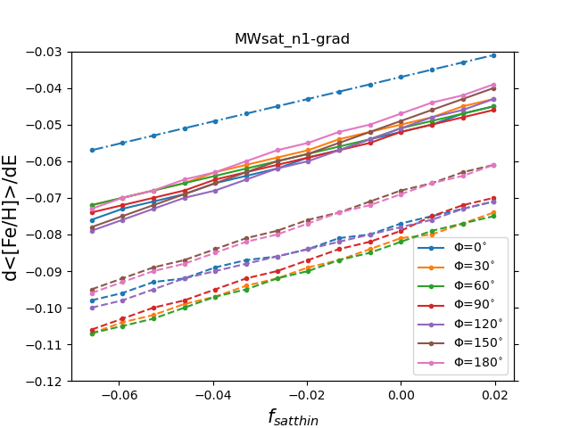
Figure 11: Relation between the slope of the initial radial metallicity gradient in the satellite thin disc ($f_{satthin}$) and the slope of the metallicity gradient in the final distribution of all the thin disc stars in the $E-L_{z}$ space as a function of energy (d¡[Fe/H]¿/dE), in the total volume of the simulation (solid lines) and in the restricted solar-like volume (dashed line). The case $\phi_{orb}=0^{\circ}$ features also the dashed-dot-curve described in the Section 3.4.

4 Conclusions

In this paper we have analysed N-body simulations of the accretion of a satellite galaxy onto a MW-type galaxy (mass ratio of the accretion 1:10), to explore to what extent we can couple kinematic characteristics and metallicities of stars in the halo to reconstruct the accretion history of our Galaxy. The main conclusions of our work are the following:

• We confirm earlier results that accreted stars from $\sim$1:10 mass ratio satellites (Jean-Baptiste et al., 2017; Koppelman et al., 2020; Amarante et al., 2022; Khoperskov et al., 2023c) and that in particular stars deposited at higher energies have on average different metallicities than those of stars that at the end of the accretion process end up to be more gravitationally bound to the Milky Way (Amarante et al., 2022; Khoperskov et al., 2023a, d).

• Because satellite stars with different metallicities can be deposited in different regions of the $E-L_{z}$ space, this implies that a single $\sim$1:10 accretion can manifest with different MDFs, in different regions of the $E-L_{z}$ space.

• Groups of stars with different $E$, $L_{z}$ and metallicities may be interpreted as originating from different satellite galaxies, but our analysis shows that these interpretations are not physically motivated .

• When the analysis is restricted to a solar-like volume, we cannot capture anymore the very metal-rich (or metal-poor, depending on the initial conditions in the satellite) accreted stars found at very high energies. This implies that the MDF of the GSE may still exhibit biases.

• Reconstructing the Galactic accretion history through mass-metallicity relations using the MDF mean values of single clumps can be very misleading. For example, a single merger of $5\times 10^{10}$ mass galaxy can be erroneously interpreted as three of $\sim 10^{7}$, $\sim 10^{8.4}$ and $\sim 10^{9.4}$ masses.

• From the metallicity gradient in the $E-L_{z}$ space as a function of energy one can retrieve information about the initial conditions of the radial metallicity gradient in the original satellite.

As we show, coupling kinematic information with the MDFs to reconstruct the accretion history of the MW can bias the reconstructed merger tree towards increasing the number of past accretions and decreasing the masses of the progenitor galaxies.

A number of possible accretion events have been proposed in the literature by making use of this approach, and our analysis reinforces previous suggestions that at least some of these accretion events are disputable. Indeed, we have shown how a single massive accretion can produce MDFs whose characteristics change across the $E-L_{z}$ plane. In a scenario in which the MW may have experienced more than a single significant accretion in its past, it is clear that the interpretation of these spaces, and related MDFs, becomes even more challenging. To this respect, we recall the reader that even the Gaia Sausage-Enceladus merger initially discovered in a solar vicinity volume (Nissen & Schuster, 2010) was suspected to be made by more than a single galaxy, already at the time of its “local” discovery (see discussion in Nissen & Schuster, 2010). New evidence have recently been published about the possibility that these accretion event hides indeed multiple ones (Donlon & Newberg, 2023; Nissen et al., 2023). Ultimately, the overall the merger tree of the MW is still far to be robustly established, and - even more importantly - we still need to establish sound methods to discriminate among accretion scenarios.

Appendix A MDF in different regions of the $E-L_{z}$ space for different $\phi_{orb}$

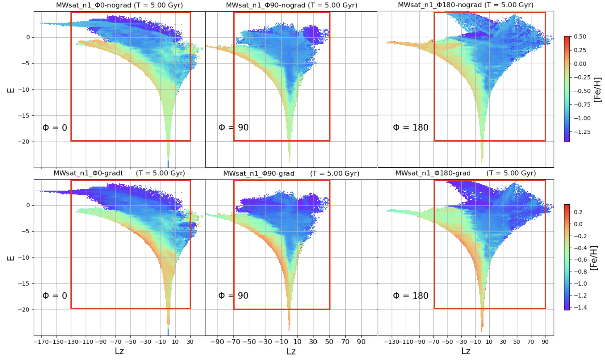
Figure 12: Same as Figure 8, but for the case of $\phi_{orb}=0^{\circ},90^{\circ},180^{\circ}$ in the first, second and third column, respectively. First row for the case of an initial vertical metallicity gradient only and second row for an initial additional radial metallicity gradient.

We wanted to check for the dependence of the results concerning the MDFs analysis on the orbital parameter $\phi_{orb}$, i.e. the initial inclination of the satellite orbital plane. We consider three more cases for a planar, polar and retrograde orbit: $\phi_{orb}=0^{\circ},90^{\circ},180^{\circ}$ and we perform the same analysis made for the $\phi_{orb}=150^{\circ}$ case (described in Section 3.2). In Figure 12, we show the final total distribution in the $E-L_{z}$ plane color-coded by mean metallicity (described in Section 3.1), where the different columns correspond to $\phi_{orb}=0^{\circ},90^{\circ},180^{\circ}$ and the two different rows correspond to the ”nograd” and ”grad” cases, respectively. The grid shows the splitting of the $E-L_{z}$ regions in which we analysed the MDFs and the red rectangle indicates the ones reported in the following Figures 13, 14 and 15. Every plot then shows the MDF considering all the stars in the region (in black), the MDF of the Milky Way-type stars only (in red) and the MDF for the satellite stars only (in blue), all normalised in order to compare means, peaks and shapes. The solid lines show the mean of the distribution, while the dotted ones show its median. In all these Figures, different rows show the MDFs for a fixed interval of energy, which in top-bottom direction are: i) 0 ¡ E ¡ 5, ii) -5 ¡ E ¡ 0, iii) -10 ¡ E ¡ -5, iv) -15 ¡ E ¡ -10, v) -20 ¡ E ¡ -15.Different columns show, instead, the MDFs for a fixed interval of angular momentum (increasing in the left-right direction). Angular momentum intervals column by column, which from left to right are, for Figure 13: i) -130 ¡ $L_{z}$ ¡ -110, ii) -110 ¡ $L_{z}$ ¡ -90, iii) -90 ¡ $L_{z}$ ¡ -70, iv) -70 ¡ $L_{z}$ ¡ -50, v) -50 ¡ $L_{z}$ ¡ -30, vi) -30 ¡ $L_{z}$ ¡ -10, vii) -10 ¡ $L_{z}$ ¡ 10, viii) 10 ¡ $L_{z}$ ¡ 30; for Figure 14: i) -70 ¡ $L_{z}$ ¡ -50, ii) -50 ¡ $L_{z}$ ¡ -30, iii) -30 ¡ $L_{z}$ ¡ -10, iv) -10 ¡ $L_{z}$ ¡ 10, v) 10 ¡ $L_{z}$ ¡ 30, vi) 30 ¡ $L_{z}$ ¡ 50; for Figure 15: i) -70 ¡ $L_{z}$ ¡ -50, ii) -50 ¡ $L_{z}$ ¡ -30, iii) -30 ¡ $L_{z}$ ¡ -10, iv) -10 ¡ $L_{z}$ ¡ 10, v) 10 ¡ $L_{z}$ ¡ 30, vi) 30 ¡ $L_{z}$ ¡ 50, vii) 50 ¡ $L_{z}$ ¡ 70, viii) 70 ¡ $L_{z}$ ¡ 90. The aim was to analyse the MDF in different regions of the $E-L_{z}$ space, in order to find any trend in their means, peaks and overall shape as a function of the region considered, for instance fixing the value of the energy and varying the one of the angular momentum, and vice-versa. All the simulations show a lower value of mean metallicity the higher the energy.

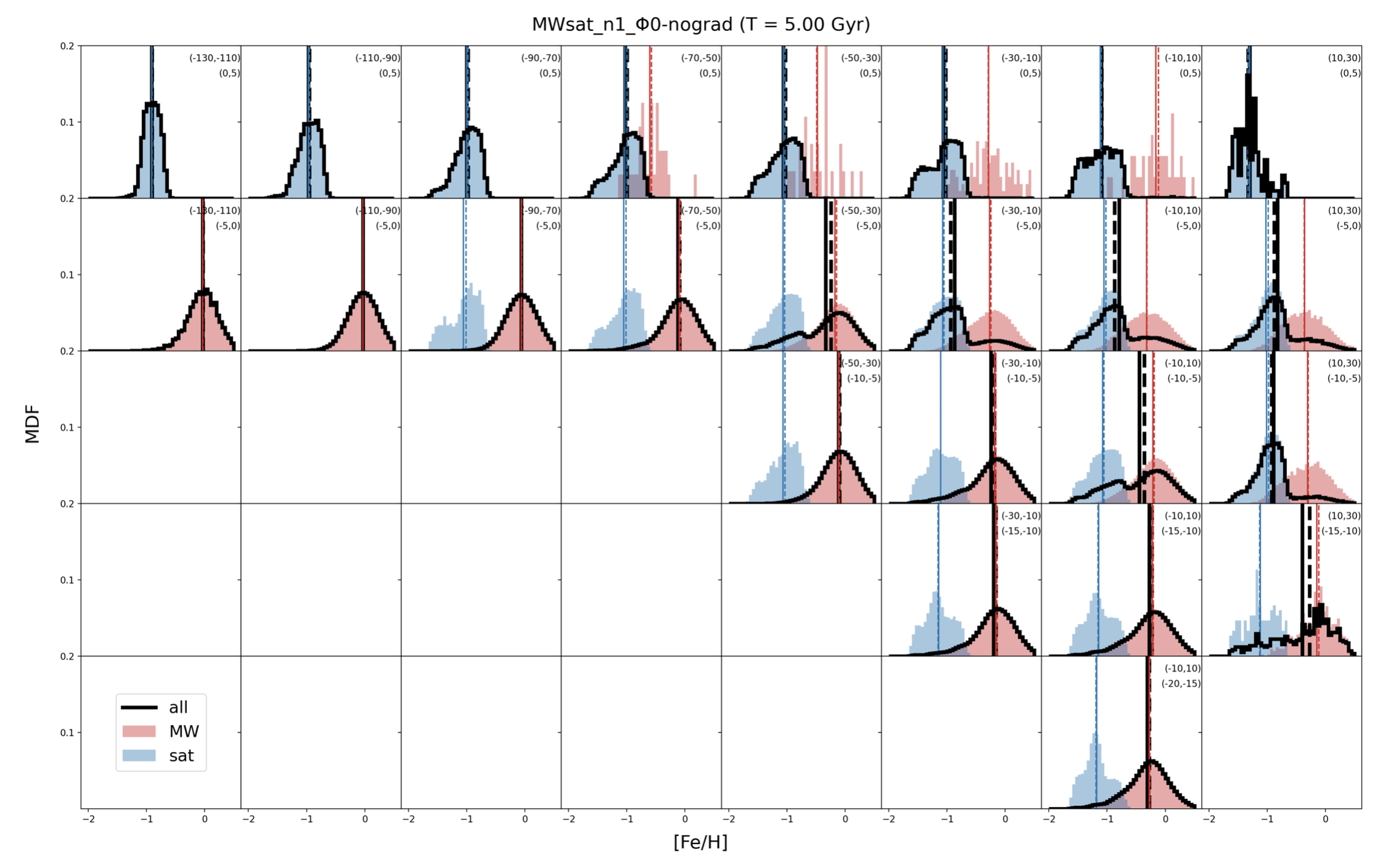
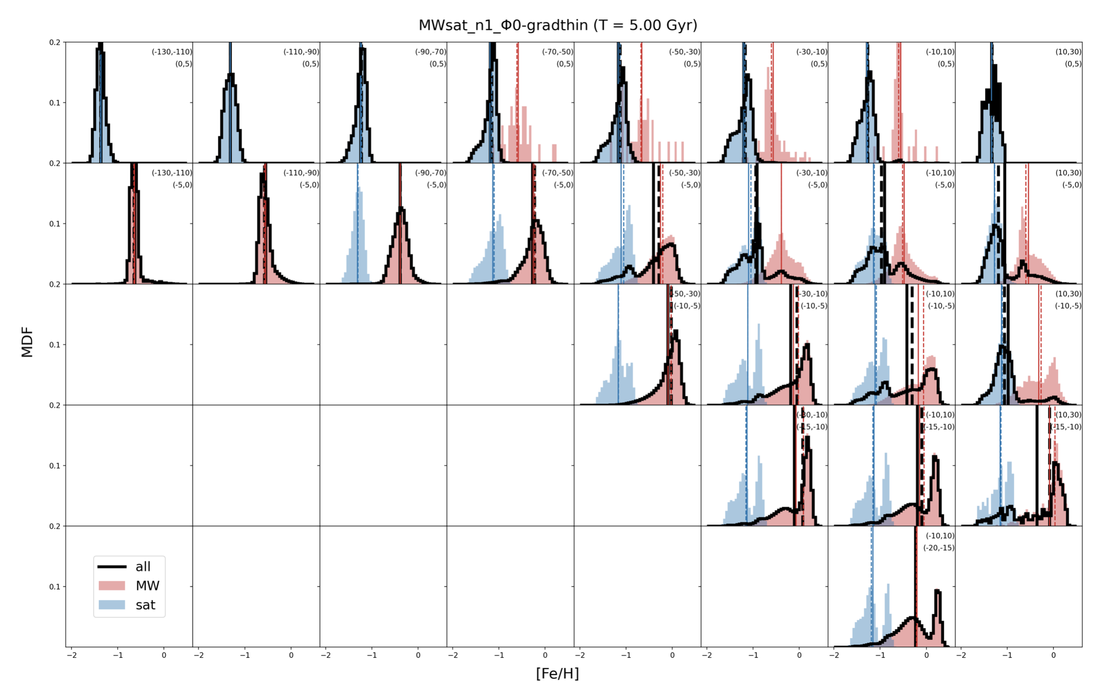
Figure 13: Same as Figure 9, but for the case of $\phi_{orb}=0^{\circ}$. Upper panel for the case of an initial vertical metallicity gradient only and lower panel for an initial additional radial metallicity gradient.

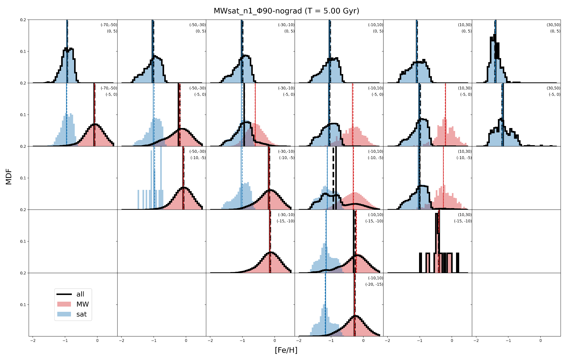
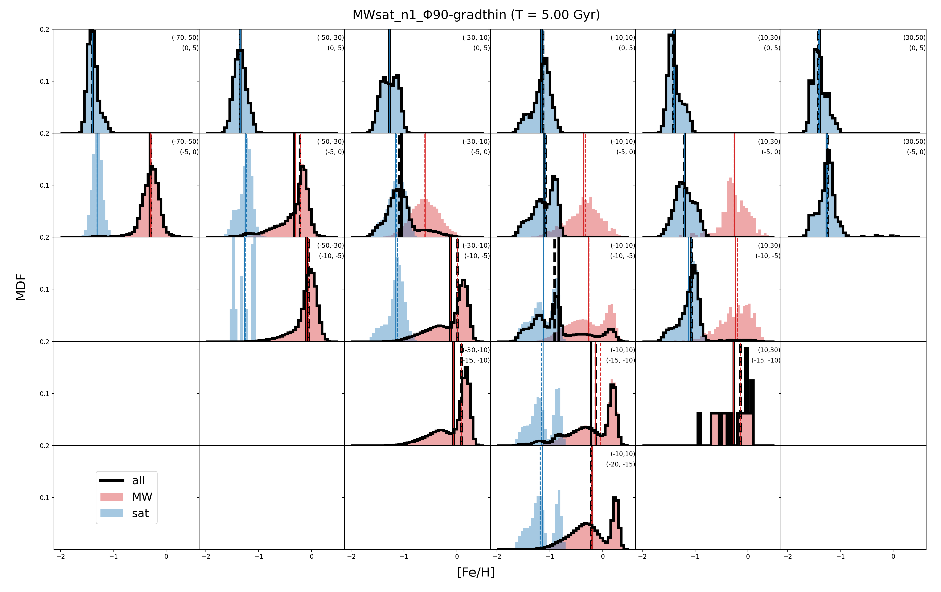
Figure 14: Same as Figure 9, but for the case of $\phi_{orb}=90^{\circ}$. Upper panel for the case of an initial vertical metallicity gradient only and lower panel for an initial additional radial metallicity gradient.

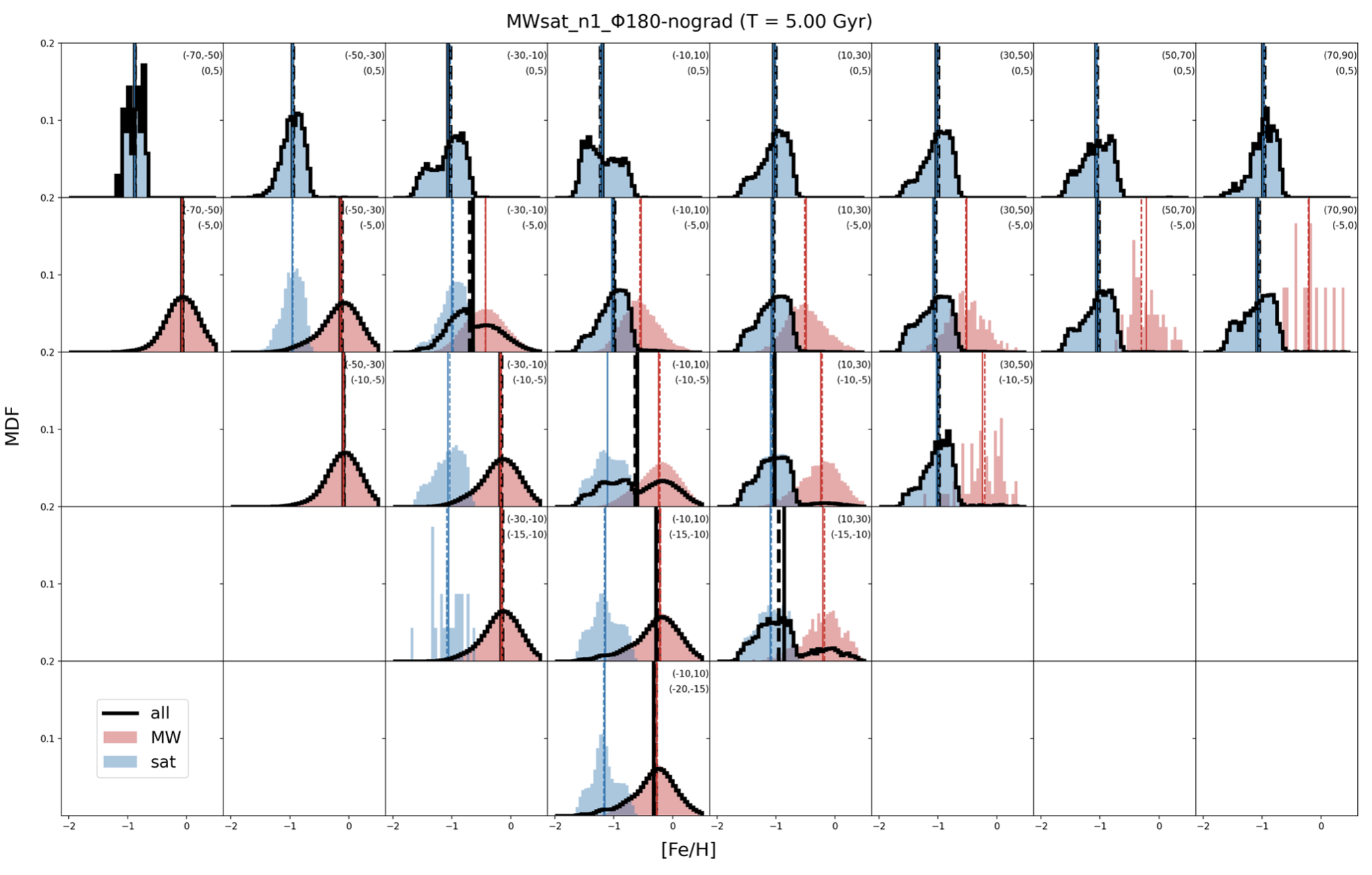
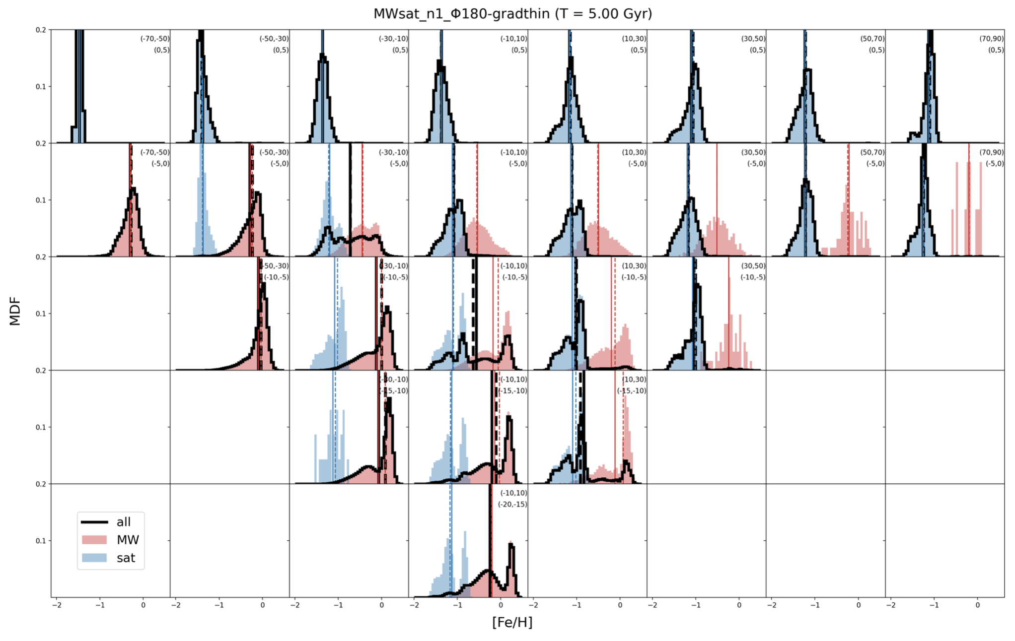
Figure 15: Same as Figure 9, but for the case of $\phi_{orb}=180^{\circ}$. Upper panel for the case of an initial vertical metallicity gradient only and lower panel for an initial additional radial metallicity gradient.