Abstract

In this paper, we investigate the quantum dynamics of scalar and oscillator fields in a topological defect space-time background under the influence of rainbow gravity’s. The rainbow gravity’s are introduced into the considered cosmological space-time geometry by replacing the temporal part $dt\to\frac{dt}{\mathcal{F}(\chi)}$ and the spatial part $dx^{i}\to\frac{dx^{i}}{\mathcal{H}(\chi)}$, where $\mathcal{F},\mathcal{H}$ are the rainbow functions and $\chi=E/E_{p}$. We derived the radial equation of the Klein-Gordon equation and its oscillator equation under rainbow gravity’s in topological space-time. To obtain eigenvalue of the quantum systems under investigations, we set the rainbow functions $\mathcal{F}(\chi)=1$ and $\mathcal{H}(\chi)=\sqrt{1-\beta\,\chi^{p}}$, where $p=1,2$. We solve the radial equations through special functions using these rainbow functions and analyze the results. In fact, it is shown that the presence of cosmological constant, the topological defect parameter $\alpha$, and the rainbow parameter $\beta$ modified the energy spectrum of scalar and oscillator fields in comparison to the results obtained in flat space.

Faizuddin Ahmed
Department of Physics, University of Science & Technology Meghalaya, Ri-Bhoi, 793101, India
Abdelmalek Bouzenada
Laboratory of Theoretical and Applied Physics, Echahid Cheikh Larbi Tebessi University, Algeria

Keywords: Modified theories of gravity; Quantum fields in curved space-time; Relativistic wave equations, Solutions of wave equations: bound-state, special functions.

PACS numbers: 04.50.Kd; 04.62.+v; 03.65.Pm; 03.65.Ge; 02.30.Gp

1 Introduction

Rainbow gravity represents a semi-classical exploration of high-energy phenomena in quantum gravity. It achieves this by introducing higher-order terms in the energy-momentum dispersion relation through the use of rainbow functions. These functions, linked to the ratio between the energy of a test particle (such as a boson or fermion) and the Planck energy, lead to a breakdown of Lorentz symmetry at this particular energy scale [1, 2, 3]. The rainbow functions play a crucial role in governing deviations from the conventional relativistic, Minkowskian expressions. Consequently, to establish this theoretical framework, the spacetime metric must also exhibit energy dependence, with this dependence intensifying as the energy of the probing particle approaches the Planck scale.

The concept known as rainbow gravity, which is essentially an effective theory of quantum gravity, can be viewed as an endeavor to embody the generalized curvature of spacetime in the context of Doubly Special Relativity [1, 2, 4, 5]. In the realm of Doubly Special Relativity, modifications in dispersion relations are accompanied by alterations in Lorentz symmetries to establish an invariant energy (length) scale, alongside the conventional invariant velocity of light (especially at lower energies). As such, rainbow gravity is grounded on the foundational principle that these two quantities remain invariant, with the fixed energy scale being identified as the Planck energy [1, 2, 3, 4, 5].

Rainbow gravity holds significant importance as it finds applications across various physical systems, bringing modifications to classical theories. An illustrative example is its integration with Friedmann–Robertson–Walker (FRW) cosmologies, explored in [6], where the potential resolution of the Big Bang singularity is investigated. Furthermore, [7] delves into the exploration of the modified Starobinsky model and the inflationary solution to motion equations using rainbow gravity. This investigation extends to the calculation of crucial parameters such as the spectral index of curvature perturbation and the tensor-to-scalar ratio. Expanding its scope, rainbow gravity has also been employed to study phenomena like the deflection of light, photon time delay, gravitational red-shift, and the weak equivalence principle, as detailed in [8].

Recent investigations into the behavior of relativistic Klein-Gordon (KG) and Dirac particles have delved into diverse spacetimes within the framework of rainbow gravity. Noteworthy examples include studies conducted in a cosmic string spacetime background, where Bezerra et al. [9] examined Landau levels through Schrödinger and KG equations. Additionally, Bakke and Mota [10, 11] explored Dirac oscillators, Sogut et al. [12] investigated the quantum dynamics of photons, and Kangal et al. [13] studied KG particles in a topologically trivial Gödel-type spacetime under rainbow gravity. Mustafa explored KG-Coulomb particles in a cosmic string rainbow gravity spacetime [14], and massless KG-oscillators in Som-Raychaudhuri cosmic string spacetime within finely tuned rainbow gravity [15]. These studies aim to unravel the dynamics of both relativistic and non-relativistic particles in curved spacetime, providing insights into the intricate interplay between quantum mechanics and general relativity. The pursuit of exact or quasi-exact solutions for such systems illuminates the captivating influence of curved spacetime on the spectroscopic structure of relativistic particles, with implications in cosmology, the geometrical theory of topological defects, and the study of black holes and wormholes, among other areas.

In gravity’s rainbow, the metric describing the geometry of spacetime depends on the energy of the test particle used to probe the structure of that space-time. So, the geometry of space-time is represented by a family of energy dependent metrics forming a rainbow of metrics. In gravity’s rainbow, the energy–momentum dispersion relation is modified by energy dependent rainbow functions, $\mathcal{F}(\chi)$ and $\mathcal{H}(\chi)$, where $\chi=E/E_{p}$, such that [16]

$$E^{2}\,\mathcal{F}^{2}(\chi)-p^{2}\,\mathcal{H}^{2}(\chi)=m^{2}\,.$$ (1)

As it is required that the usual energy-momentum dispersion relation is recovered in the infrared (IR) limit, these rainbow functions are required to satisfy

$$\lim_{\chi\to 0}\mathcal{F}(\chi)\to 1,\quad\lim_{\chi\to 0}\mathcal{H}(\chi)\to 1.$$ (2)

The energy dependent metric in gravity’s rainbow can be written as [17]

$$g^{\mu\nu}(\chi)=e^{\mu}_{a}(\chi)\,e^{\nu}_{b}(\chi)\,\eta^{ab},$$ (3)

where $\eta^{\mu}_{a}$ is the orthonormal tetrad fields, $\eta^{ab}$ is the Minkowski metric, and $E$ is the energy of the probing particle. The rainbow functions are defined using this energy $E$ that cannot exceed the Planck energy $E_{p}$.

In the literature of gravity’s rainbow, many proposals exist for the rainbow functions $\mathcal{F}(\chi)$ and $\mathcal{H}(\chi)$ [18, 19, 20, 21, 22, 23, 24, 25, 26, 27, 28, 29, 30, 31, 32, 33, 34, 35, 36, 37]. The choice of the rainbow functions is supposed to be based on phenomenological motivations. We use one of the most interesting and most studied rainbow functions that was proposed in Refs. [16, 38, 39]

$$\mathcal{F}(\chi)=1,\quad\mathcal{H}=\sqrt{1-\beta\,\chi^{p}}\quad(p=1,2).$$ (4)

The modified dispersion relation with these functions is compatible with some results from non-critical string theory, loop quantum gravity and $\kappa$-Minkowski non-commutative space-time. This modified dispersion relation has been used to study the dispersion of electromagnetic waves from gamma ray bursters [39]. It also solves the ultra high energy gamma rays paradox [40, 41], and the paradox of the 20 TeV gamma rays from the galaxy Markarian 501 [40, 42]. In addition, this MDR provides stringent constraints on deformations of special relativity and Lorentz violations [43, 44].

Addressing the Einstein-Maxwell equations, Bonnor formulated an exact static solution, discussed in detail for its physical implications [45]. Melvin later revisited this solution, leading to the currently recognized Bonnor-Melvin magnetic universe [46]. An axisymmetric Einstein-Maxwell solution, incorporating a varying magnetic field and a cosmological constant, was constructed in [47]. This electrovacuum solution was subsequently expanded upon in [47, 48]. This analysis primary focus on Bonnor-Melvin-type universe featuring a cosmological constant, discussed in detailed in Ref. [49]. The line-element describing this magnetic universe in the chart $(t,\rho,\phi,z)$ is given by [49]

$$ds^{2}=-dt^{2}+dz^{2}+\frac{1}{2\,\Lambda}\,\Big{(}d\rho^{2}+\sin^{2}\rho\,d\phi^{2}\Big{)},$$ (5)

where $\Lambda$ denotes the cosmological constant and the magnetic field strength is given by $B=\sqrt{2}\,\sin\rho$.

We now introduces a cosmic string into the above line-element by performing a coordinate transformation $\phi\to\alpha\,\phi$, where $\alpha$ is the cosmic string parameter which produces an angular deficit with the ranges $0<\alpha<1$. Therefore, the above line-element (5) under this transformation becomes

$$ds^{2}=-dt^{2}+dz^{2}+\frac{1}{2\,\Lambda}\,\Big{(}d\rho^{2}+\alpha^{2}\,\sin^{2}\rho\,d\phi^{2}\Big{)},$$ (6)

where now the magnetic field strength becomes $B=\sqrt{2}\,\alpha\,\sin\rho$ which is $\alpha$ times the original field strength but decreases by this amount.

Finally, the rainbow gravity’s effect is introduced into this space-time (6) by replacing the temporal part $dt\to\frac{dt}{\mathcal{F}(\chi)}$ and the spatial part $dx^{i}\to\frac{dx^{i}}{\mathcal{H}(\chi)}$, where $\mathcal{F},\mathcal{H}$ are the rainbow functions stated earlier. Therefore, the space-time (6) under rainbow gravity’s can be described by the following line-element [50, 51]

$$ds^{2}=-\frac{dt^{2}}{\mathcal{F}^{2}(\chi)}+\frac{1}{\mathcal{H}^{2}(\chi)}\Bigg{[}dz^{2}+\frac{1}{2\,\Lambda}\,\Big{(}d\rho^{2}+\alpha^{2}\,\sin^{2}\rho\,d\phi^{2}\Big{)}\Bigg{]}.$$ (7)

One can evaluate the magnetic field strength for the modified topological defect cosmological space-time (7) and it is given by $\mathcal{B}=\frac{\alpha}{\sqrt{2}\,\mathcal{H}(\chi)}\,\sin\rho$ which depends on the rainbow function. For $\chi\to 0$, we will get back the topological defect cosmological space-time (6).

The exploration of rainbow gravity’s implications in quantum mechanical problems has attracted much attention in current times. Various studies have delved into the effects of rainbow gravity in different quantum systems, including the Dirac oscillator in cosmic string space-time [52], scalar fields in a wormhole background with cosmic strings [53], quantum motions of scalar particles [54], and the behavior of spin-1/2 particles in a topologically trivial Gödel-type space-time [55]. Additionally, investigations have extended to the motions of photons in cosmic string space-time [56], and the generalized Duffin-Kemmer-Petiau equation with non-minimal coupling in cosmic string space-time [57].

Our motivation is to study the relativistic quantum motions of scalar and oscillator fields in a topological defect cosmological space-time under the influence of rainbow gravity’s. It is well-known that the presence of rainbow gravity’s in a space-time alter its geometrical characteristics, and hence, behaviours of quantum particles in this geometry background would definitely changes. We study this quantum mechanical problems by choosing two pairs of rainbow functions by considering $p=1,2$ in Eq. (4). In fact, we show that the solutions of the relativistic wave equation via the Klein-Gordon and its oscillator fields are influenced by the cosmological constant $\Lambda$, the topological defect parameter $\alpha$ and the rainbow parameter $\beta$. Throughout this paper, we use the system of units, where $\hbar=c=G=1$.

2 Scalar fields in topological defect cosmological space-time

In this part, we consider the physical environment of rainbow gravity effects on the relativistic quantum motions of scalar particles described by the Klein-Gordon equation in the background of axisymmetric Einstein-Maxwell solution with a cosmological. We begin this part by writing the relativistic wave equation describing the quantum motions of scalar particles given by [50, 51, 58]

$$\Bigg{[}-\frac{1}{\sqrt{-g}}\,\partial_{\mu}\,\Big{(}\sqrt{-g}\,g^{\mu\nu}\,\partial_{\nu}\Big{)}+M^{2}\Bigg{]}\,\Psi=0,$$ (8)

where $M$ is the rest mass of the particles, $g$ is the determinant of the metric tensor $g_{\mu\nu}$ with its inverse $g^{\mu\nu}$.

The covariant ($g_{\mu\nu}$) and contravariant form ($g_{\mu\nu}$) of the metric tensor for the space-time (7) are given by

$$g_{\mu\nu}=\mbox{diag}\Big{(}-\frac{1}{\mathcal{F}^{2}(\chi)},\frac{1}{2\,\Lambda\,\mathcal{H}^{2}(\chi)},\frac{\alpha^{2}\,\sin^{2}\rho}{2\,\Lambda\,\mathcal{H}^{2}(\chi)},\frac{1}{\mathcal{H}^{2}(\chi)}\Big{)},$$

$$g^{\mu\nu}=\mbox{diag}\Big{(}-\mathcal{F}^{2}(\chi),2\,\Lambda\,\mathcal{H}^{2}(\chi),\frac{2\,\Lambda\,\mathcal{H}^{2}(\chi)}{\alpha^{2}\,\sin^{2}\rho},\mathcal{H}^{2}(\chi)\Big{)}.$$ (9)

The determinant of the metric tensor for the space-time (7) is given by

$$det\,(g_{\mu\nu})=g=-\frac{\alpha^{2}\,\,\sin^{2}\rho}{4\,\Lambda^{2}\,\mathcal{H}^{6}(\chi)\,\mathcal{F}^{2}(\chi)}\,.$$ (10)

Therefore, the KG-equation (8) in the space-time (6) can be expressed in the following differential equation:

$$\Bigg{[}-\mathcal{F}^{2}\,\frac{d^{2}}{dt^{2}}+2\,\Lambda\,\mathcal{H}^{2}\,\Bigg{\{}\frac{d^{2}}{d\rho^{2}}+\frac{1}{\tan\rho}\,\frac{d}{d\rho}+\frac{1}{\alpha^{2}\,\sin^{2}\rho}\,\frac{d^{2}}{d\phi^{2}}\Bigg{\}}+\mathcal{H}^{2}\,\frac{d^{2}}{dz^{2}}-M^{2}\Bigg{]}\,\Psi=0\,.$$ (11)

In quantum mechanical system, the total wave function is always expressible in terms of different variables. In our case, we choose the following ansatz of the total wave function $\Psi$ in terms of different variable functions $\psi(x)$ and $\Theta(\theta)$ as follows:

$$\Psi=\exp(-i\,E\,t)\,\exp(i\,\ell\,\phi)\,\exp(i\,k\,z)\,\psi(\rho),$$ (12)

where $E$ is the particles energy, $\ell=0,\pm\,1,\pm\,2,....$ are the eigenvalues of the angular quantum number, and $k$ is an arbitrary constant.

Substituting the total wave function (12) into the differential equation (11), we obtain the differential equations for $\psi(\rho)$ as follows:

$$\psi^{\prime\prime}+\frac{1}{\tan\rho}\,\psi^{\prime}+\Bigg{[}\frac{(\mathcal{F}^{2}\,E^{2}-M^{2})}{2\,\Lambda\,\mathcal{H}^{2}}-\frac{k^{2}}{2\,\Lambda}-\frac{\iota^{2}}{\sin^{2}\rho}\Bigg{]}\,\psi=0,\quad\iota=\frac{|\ell|}{\alpha}\,.$$ (13)

We solve the above equation taking an approximation of the trigonometric function up to the first order, that is, $\sin\rho\approx\rho$, $\tan\rho\approx\rho$. Therefore, the radial wave equation (13) reduces to the following form:

$$\psi^{\prime\prime}+\frac{1}{\rho}\,\psi^{\prime}+\Big{(}\eta^{2}-\frac{\iota^{2}}{\rho^{2}}\Big{)}\,\psi=0,$$ (14)

where

$$\eta=\sqrt{\frac{(\mathcal{F}^{2}\,E^{2}-M^{2})}{2\,\Lambda\,\mathcal{H}^{2}}-\frac{k^{2}}{2\,\Lambda}}\,.$$ (15)

Equation (14) is the second-order Bessel equation whose solutions are well-known given by $\psi(\rho)=c_{1}\,J_{\iota}(\eta\,\rho)+c_{2}\,Y_{\iota}(\eta\,\rho)$. It si also known that the Bessel function of first kind $J$ is finite and the second kind $Y$ diverge at the origin $\rho=0$. Therefore, employing the condition that the wave function $\psi\to 0$ at $\rho=0$ implies that $c_{2}=0$. Therefore, the regular solution at the origin is given by

$$\psi(\rho)=c_{1}\,J_{\iota}(\eta\,\rho)\,.$$ (16)

At large distance, the Bessel function of the first kind in the asymptotic form will be [59, 60]

$$J_{\iota}(\eta\,\rho)\propto\cos\Big{(}\eta\,\rho-\frac{\pi\,\iota}{2}-\frac{\pi}{4}\Big{)}\,.$$ (17)

Now, we want to restrict the motion of quantum particles to a region where a hard-wall confining potential is present. This type of confinement is important because it is a very good approximation to consider when discussing the quantum properties of a gas molecule system and other particles, which are necessarily confined in a box of certain dimensions. The hard-wall coffining potential has been studied by many researchers in the quantum systems Refs. [61, 62, 63, 64, 65, 66, 67, 68, 69, 70]. According to the Dirichlet boundary condition, the radial wave function vanishes at some finite distance $\rho=\rho_{0}$, that is,

$$\psi(\rho=\rho_{0})=0\,.$$ (18)

Thus, using Eq. (17) into the Eq. (16) and finally employing condition (18), we obtain

$$\Big{(}\eta\,\rho-\frac{\pi\,\iota}{2}-\frac{\pi}{4}\Big{)}=(2\,n+1)\,\frac{\pi}{2}\quad(n=0,1,2,...).$$ (19)

Simplification of the above relation results

$$\mathcal{F}^{2}(\chi)\,E^{2}-M^{2}=\mathcal{H}^{2}(\chi)\,\Bigg{[}k^{2}+2\,\Lambda\,\Big{(}n+\frac{|m|}{2\,\alpha}+\frac{3}{4}\Big{)}^{2}\,\frac{\pi^{2}}{\rho^{2}_{0}}\Bigg{]}\,.$$ (20)

In this analysis, we choose two pairs of rainbow functions as follows and obtain the energy spectrum of the scalar particles.

Case A: $\mathcal{F}(\chi)=1$ and $\mathcal{H}(\chi)=\sqrt{1-\beta\,\chi}$, where $\chi=\frac{|E|}{E_{p}}$

In this case, we choose a pair of rainbow functions given by

$$\mathcal{F}(\chi)=1,\quad\mathcal{H}(\chi)=\sqrt{1-\beta\,\chi},\quad\chi=\frac{E}{E_{p}}\,.$$ (21)

Substituting this pair of rainbow function into the energy eigenvalue relation (20), we obtain

$$E^{2}_{n,\ell}-M^{2}=\Big{(}1-\frac{\beta}{E_{p}}\,|E_{n,\ell}|\Big{)}\,\Bigg{[}k^{2}+2\,\Lambda\,\Big{(}n+\frac{|\ell|}{2\,\alpha}+\frac{3}{4}\Big{)}^{2}\,\frac{\pi^{2}}{\rho^{2}_{0}}\Bigg{]}\,.$$ (22)

For $|E_{n,\ell}|=E_{n,\ell}$, from the above relation we obtain the compact expression of the energy eigenvalue given by

$$E^{\pm}_{n,\ell}=-\Big{(}\frac{\beta}{E_{p}}\Big{)}\,\frac{\Delta_{n,\ell}}{2}\pm\sqrt{\Big{(}\frac{\beta}{E_{p}}\Big{)}^{2}\,\frac{\Delta^{2}_{n,\ell}}{4}+M^{2}+\Delta_{n,\ell}}\,,$$ (23)

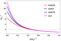
(a)

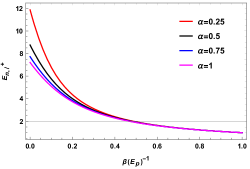
(b)

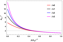
(c)

Figure 1: Positive energy $E_{n,\ell}^{+}$ in (23) where $n=K=M=1$

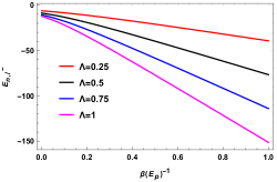
(a)

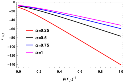
(b)

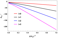
(c)

Figure 2: Negative energy $E_{n,\ell}^{-}$ in (23) where $n=K=M=1$

where

$$\Delta_{n,\ell}=k^{2}+2\,\Lambda\,\Big{(}n+\frac{|\ell|}{2\,\alpha}+\frac{3}{4}\Big{)}^{2}\,\frac{\pi^{2}}{\rho^{2}_{0}}\,.$$ (24)

For $|E_{n,\ell}|=-E_{n,\ell}$, from the above relation we obtain the compact expression of the energy eigenvalue given by

$$E^{\pm}_{n,\ell}=\Big{(}\frac{\beta}{E_{p}}\Big{)}\,\frac{\Delta_{n,\ell}}{2}\pm\sqrt{\Big{(}\frac{\beta}{E_{p}}\Big{)}^{2}\,\frac{\Delta^{2}_{n,\ell}}{4}+M^{2}+\Delta_{n,\ell}}.$$ (25)

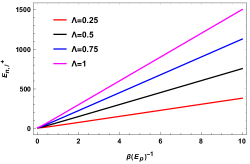
(a)

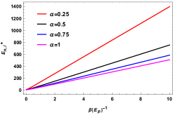
(b)

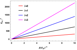
(c)

Figure 3: The energy spectrum $E_{n,\ell}^{+}$ of Eq. (25), where $n=\rho_{0}=k=M=1$

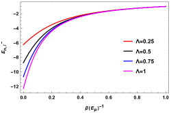
(d)

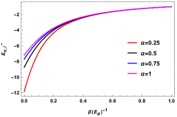
(e)

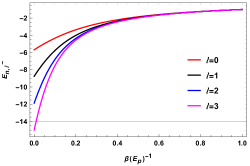
(f)

Figure 4: The energy spectrum $E_{n,\ell}^{-}$ of Eq. (25), where $n=\rho_{0}=k=M=1$

Equations (23) and (25) are the relativistic approximate energy eigenvalue of scalar particles associated with the modes $\{n,\ell\}$ in the background of topological defect cosmological space-time (7) for the chosen rainbow function $\mathcal{F}(\chi)=1$ and $\mathcal{H}(\chi)=\sqrt{1-\beta\,\chi}$.

We have plotted the energy spectrum of scalar particles given in Eq. (23) in Figures 1-2 and Eq. (25) in Figures 3-4 for different values of the cosmological constant $\Lambda$, the topological parameter $\alpha$, and the angular quantum number $\ell$ and shows their behaviour either increasing or decreasing trend.

Case B: $\mathcal{F}(\chi)=1$ and $\mathcal{H}(\chi)=\sqrt{1-\beta\,\chi^{2}}$, where $\chi=\frac{|E|}{E_{p}}$

In this case, we choose a pair of rainbow functions given by

$$\mathcal{F}(\chi)=1,\quad\mathcal{H}(\chi)=\sqrt{1-\beta\,\chi^{2}},\quad\chi=\frac{|E|}{E_{p}}\,.$$ (26)

Substituting this pair of rainbow function into the energy eigenvalue relation (20), we obtain

$$E^{2}_{n,\ell}-M^{2}=(1-\beta\,\chi^{2})\,\Bigg{[}k^{2}+2\,\Lambda\,\Big{(}n+\frac{|\ell|}{2\,\alpha}+\frac{3}{4}\Big{)}^{2}\,\frac{\pi^{2}}{\rho^{2}_{0}}\Bigg{]}\,.$$ (27)

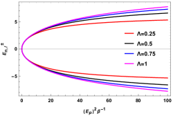
(a)

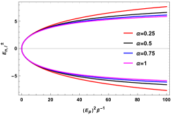
(b)

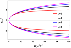
(c)

Figure 5: The energy spectrum $E_{n,\ell}^{\pm}$ of Eq. (28), where $n=\rho_{0}=k=M=1$

Simplification of the above relation gives us the compact expression of the energy eigenvalue given by

$$E^{\pm}_{n,\ell}=\pm\sqrt{\frac{M^{2}+k^{2}+2\,\Lambda\,\Big{(}n+\frac{|\ell|}{2\,\alpha}+\frac{3}{4}\Big{)}^{2}\,\frac{\pi^{2}}{\rho^{2}_{0}}}{1+\frac{\beta}{E^{2}_{p}}\,\Big{[}k^{2}+2\,\Lambda\,\Big{(}n+\frac{|\ell|}{2\,\alpha}+\frac{3}{4}\Big{)}^{2}\,\frac{\pi^{2}}{\rho^{2}_{0}}\Big{]}}}.$$ (28)

Equation (28) is the relativistic approximate energy eigenvalue of scalar particles associated with the modes $\{n,\ell\}$ in the background of topological defect cosmological space-time (7) for the chosen rainbow function $\mathcal{F}(\chi)=1$ and $\mathcal{H}(\chi)=\sqrt{1-\beta\,\chi^{2}}$.

We have plotted the energy spectrum of scalar particles given in Eq. (28) in Figure 5 for different values of the cosmological constant $\Lambda$, the topological parameter $\alpha$, and the angular quantum number $\ell$ and shows their behaviour.

3 Quantum oscillator field in topological defect cosmological space-time

In this part, dynamics of quantum oscillator field described by the Klein-Gordon oscillator under the environment of rainbow gravity’s is investigated in curved space-time produced by a magnetic field given by the metric (7). The Klein-Gordon oscillator equation is studied by substituting the momentum four-vector $\partial_{\mu}\to(\partial_{\mu}+M\,\omega\,X_{\mu})$, with $X_{\mu}=(0,r,0,0)$ and $\omega$ represents the oscillator frequency. Extensive exploration investigating the dynamics of quantum oscillator field in various space-time backgrounds including Gödel and Gödel-type space-times both with and without cosmic strings have been done. Moreover, investigations have been conducted in global monopoles, cosmic string space-times (both standard and spinning), as well as in topologically trivial and non-trivial geometries (see, Refs. [71, 72, 73, 74, 75, 76, 77, 78, 79, 80, 81, 82]). The examination of the relativistic quantum oscillator field within diverse space-time backgrounds provides valuable insights into the interplay between quantum oscillation fields and the underlying cosmological geometry, offering a comprehensive understanding of the intricate dynamics involved in these scenarios.

Therefore, the relativistic wave equation describing the quantum oscillator field is given by

$$\Big{[}\frac{1}{\sqrt{-g}}\,(\partial_{\mu}+M\,\omega\,X_{\mu})\,(\sqrt{-g}\,g^{\mu\nu})\,(\partial_{\nu}-M\,\omega\,X_{\nu})\Big{]}\,\Psi=M^{2}\,\Psi\,.$$ (29)

Expressing this wave equation (29) in the space-time background (7), we obtain the following equation

$$\Bigg{[}-\mathcal{F}^{2}\,\frac{d^{2}}{dt^{2}}+2\,\Lambda\,\mathcal{H}^{2}\,\Bigg{\{}\frac{d^{2}}{d\rho^{2}}+\frac{1}{\tan\rho}\,\frac{d}{d\rho}-M\,\omega-\frac{M\,\omega\,\rho}{\tan\rho}-M^{2}\,\omega^{2}\,\rho^{2}+\frac{1}{\alpha^{2}\,\sin^{2}\rho}\,\frac{d^{2}}{d\phi^{2}}\Bigg{\}}$$

$$+\mathcal{H}^{2}\,\frac{d^{2}}{dz^{2}}-M^{2}\Bigg{]}\,\Psi=0\,.$$ (30)

Substituting the wave function ansatz Eq. (12), we obtain

$$\psi^{\prime\prime}(\rho)+\frac{1}{\tan\rho}\,\psi^{\prime}(\rho)+\Bigg{[}\frac{(\mathcal{F}^{2}\,E^{2}-M^{2})}{2\,\Lambda\,\mathcal{H}^{2}}-M\,\omega-\frac{M\,\omega\,\rho}{\tan\rho}-M^{2}\,\omega^{2}\,\rho^{2}-\frac{k^{2}}{2\,\Lambda}-\frac{\iota^{2}}{\sin^{2}\rho}\Bigg{]}\,\psi(\rho)=0.$$ (31)

We solve the above equation taking an approximation of up to the first order, that is, for small values of the radial distance $r$. Therefore, the radial wave equation (31) reduces to the following form:

$$\psi^{\prime\prime}(\rho)+\frac{1}{\rho}\,\psi^{\prime}(\rho)+\Big{(}\xi^{2}-M^{2}\,\omega^{2}\,\rho^{2}-\frac{\iota^{2}}{\rho^{2}}\Big{)}\,\psi(\rho)=0,$$ (32)

where we have defined

$$\xi^{2}=\frac{(\mathcal{F}^{2}\,E^{2}-M^{2})}{2\,\Lambda\,\mathcal{H}^{2}}-\frac{k^{2}}{2\,\Lambda}-2\,M\,\omega\,.$$ (33)

Transforming the above equation (32) to a new variable via

$$s=M\,\omega\,\rho^{2}$$ (34)

we obtain

$$\psi^{\prime\prime}(s)+\frac{1}{s}\,\psi^{\prime}(s)+\Bigg{(}\frac{\xi^{2}}{4\,M\,\omega}\,\frac{1}{s}-\frac{1}{4}-\frac{\iota^{2}/4}{s^{2}}\Bigg{)}\,\psi(s)=0.$$ (35)

The requirement of the wave function is that the wave function $\psi(s)$ must be finite everywhere including at the origin $s=0$. Suppose a possible solution to this equation (35) is given as follows:

$$\psi(s)=s^{\iota/2}\,e^{-\frac{s}{2}}\,F(s),$$ (36)

where $F(s)$ is an unknown function.

Thereby, substituting this possible solution into the equation (35) results the following second-order differential equation

$$s\,F^{\prime\prime}(s)+(1+\iota-s)\,F^{\prime}(s)+\Bigg{(}\frac{\xi^{2}}{4\,M\,\omega}-\frac{1}{2}-\frac{\iota}{2}\Bigg{)}\,F(s)=0\,.$$ (37)

This is the confluent hypergeometric equation [59], which is a second-order linear homogeneous differential equation where two independent solutions can be obtained. The solution of Eq. (37) which is regular at the origin $s=0$ is given by the confluent hypergeometric function as follows:

$$F(s)={}_{1}F_{1}\Bigg{(}\frac{1}{2}+\frac{\iota}{2}-\frac{\xi^{2}}{4\,M\,\omega};1+\iota;s\Bigg{)}\,.$$ (38)

The solution of $F(s)$ is a polynomial of degree $n$ can be obtained by the Frobenius method. Note that we require regularity of the wave function in the origin $s=0$ and at infinity $s\to\infty$ in Eq. (36). The exponential term in Eq. (36) implies that $M\,\omega>0$ in order to ensure the condition of regularity of the wave function at infinity ($s\to\infty$). In terms of the coordinate $\rho$, we see that Eq. (36) is written in the form $\psi\propto\rho^{\iota}\,e^{-\frac{1}{2}\,M\,\omega\,\rho^{2}}\,{}_{1}F_{1}(M\,\omega\,\rho^{2})$. Naturally, for all possible values of $\rho$, it is easy to observe that our solution is divergent at the extremal point. However, this blow-up can be eliminated by a truncation of the power series. This procedure is equivalent to imposing the following condition:

$$\frac{1}{2}+\frac{\iota}{2}-\frac{\xi^{2}}{4\,M\,\omega}=-n\quad(n=0,1,2,3,....).$$ (39)

After simplification of the above condition, we obtain the energy relation as follows:

$$\mathcal{F}^{2}(\chi)\,E^{2}-M^{2}=\mathcal{H}^{2}(\chi)\,\Bigg{[}k^{2}+8\,M\,\omega\,\Lambda\,\Big{(}n+\frac{|\ell|}{2\,\alpha}+1\Big{)}\Bigg{]}\,.$$ (40)

The corresponding wave function (36) becomes

$$\psi_{n,\ell}(s)=s^{\frac{|\ell|}{2\,\alpha}}\,e^{-\frac{s}{2}}\,{}_{1}F_{1}\Big{(}-n;1+\frac{|\ell|}{\alpha};s\Big{)}.$$ (41)

In terms of $\rho$, we obtain the radial wave function

$$\psi_{n,\ell}(\rho)=\mathcal{C}\,(M\,\omega)^{\frac{|\ell|}{2\,\alpha}}\,\rho^{\frac{|\ell|}{\alpha}}\,e^{-\frac{1}{2}\,M\,\omega\,\rho^{2}}\,{}_{1}F_{1}\Big{(}-n;1+\frac{|\ell|}{\alpha};M\,\omega\,\rho^{2}\Big{)},$$ (42)

$\mathcal{C}$ is the normalization constant.

Below, we evaluate the energy spectrum of oscillator fields by choosing two pairs of rainbow functions considered earlier.

Case A: $\mathcal{F}(\chi)=1$ and $\mathcal{H}(\chi)=\sqrt{1-\beta\,\chi}$, where $\chi=\frac{E}{E_{p}}$

In this case, we choose a pair of rainbow functions given by

$$\mathcal{F}=1,\quad\mathcal{H}=\sqrt{1-\beta\,\chi},\quad\chi=\frac{E}{E_{p}}\,.$$ (43)

Substituting this pair of rainbow function into the energy eigenvalue relation (40), we obtain

$$E^{2}_{n,\ell}-M^{2}=\Big{(}1-\frac{\beta}{E_{p}}\,|E_{n,\ell}|\Big{)}\,\Bigg{[}k^{2}+8\,M\,\omega\,\Lambda\,\Big{(}n+\frac{|\ell|}{2\,\alpha}+1\Big{)}\Bigg{]}\,.$$ (44)

For $|E_{n,\ell}|=E_{n,\ell}$, simplification of the above relation gives us the compact expression of the energy eigenvalue given by

$$E^{\pm}_{n,\ell}=-\Big{(}\frac{\beta}{E_{p}}\Big{)}\,\frac{\Theta_{n,\ell}}{2}\pm\sqrt{\Big{(}\frac{\beta}{E_{p}}\Big{)}^{2}\,\frac{\Theta^{2}_{n,\ell}}{4}+M^{2}+\Theta_{n,\ell}}\,,$$ (45)

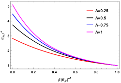
(a)

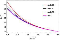
(b)

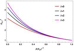
(c)

Figure 6: Positive energy $E_{n,\ell}^{+}$ in (45) where $n=\omega=K=M=1$

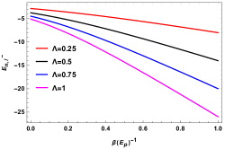
(a)

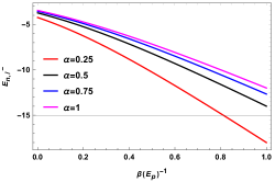
(b)

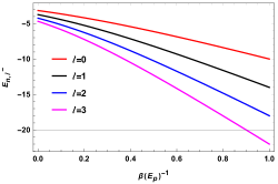
(c)

Figure 7: Negative energy $E_{n,\ell}^{-}$ in (45) where $n=\omega=K=M=1$

where

$$\Theta_{n,\ell}=k^{2}+8\,M\,\omega\,\Lambda\,\Big{(}n+\frac{|\ell|}{2\,\alpha}+1\Big{)}\,.$$ (46)

For $|E_{n,\ell}|=-E_{n,\ell}$, simplification of the above relation gives us the compact expression of the energy eigenvalue given by

$$E^{\pm}_{n,\ell}=\Big{(}\frac{\beta}{E_{p}}\Big{)}\,\frac{\Theta_{n,\ell}}{2}\pm\sqrt{\Big{(}\frac{\beta}{E_{p}}\Big{)}^{2}\,\frac{\Theta^{2}_{n,\ell}}{4}+M^{2}+\Theta_{n,\ell}}.$$ (47)

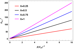
(a)

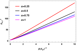
(b)

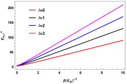
(c)

Figure 8: The energy spectrum $E_{n,\ell}^{+}$ of Eq. (47), where $n=\omega=k=M=1$

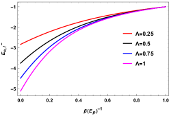
(d)

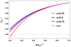
(e)

(f)

Figure 9: The energy spectrum $E_{n,\ell}^{-}$ of Eq. (47), where $n=\omega=k=M=1$

Equations (45) and (47) are the relativistic approximate energy eigenvalue of quantum oscillator fields associated with the modes $\{n,\ell\}$ in the background of topological defect cosmological space-time (7) for the chosen rainbow function $\mathcal{F}(\chi)=1$ and $\mathcal{H}(\chi)=\sqrt{1-\beta\,\chi}$.

We have plotted the energy spectrum of quantum oscillator fields given in Eq. (45) in Figures 6-7 and Eq. (47) in Figures 8-9 for different values of the cosmological constant $\Lambda$, the topological parameter $\alpha$, and the angular quantum number $\ell$ and shows their behaviour with increasing values of these parameters.

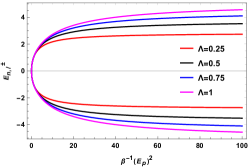
(a)

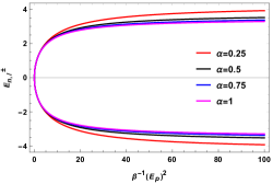
(b)

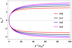
(c)

Figure 10: The energy spectrum $E_{n,\ell}^{\pm}$ of Eq. (50), where $n=\omega=k=M=1$

Case B: $\mathcal{F}(\chi)=1$ and $\mathcal{H}(\chi)=\sqrt{1-\beta\,\chi^{2}}$, where $\chi=\frac{E}{E_{p}}$

In this case, we choose a pair of rainbow functions given by

$$\mathcal{F}(\chi)=1,\quad\mathcal{H}(\chi)=\sqrt{1-\beta\,\chi^{2}},\quad\chi=\frac{E}{E_{p}}\,.$$ (48)

Substituting this pair of rainbow function into the energy eigenvalue relation (40), we obtain

$$E^{2}_{n,\ell}-M^{2}=\Big{(}1-\frac{\beta}{E^{2}_{p}}\,E^{2}_{n,\ell}\Big{)}\,\Bigg{[}k^{2}+8\,M\,\omega\,\Lambda\,\Big{(}n+\frac{|\ell|}{2\,\alpha}+1\Big{)}\Bigg{]}\,.$$ (49)

Simplification of the above relation gives us the compact expression of the energy eigenvalue given by

$$E_{n,\ell}^{\pm}=\pm\sqrt{\frac{M^{2}+k^{2}+8\,M\,\omega\,\Lambda\,\Big{(}n+\frac{|\ell|}{2\,\alpha}+1\Big{)}}{1+\frac{\beta}{E_{p}^{2}}\,\left[k^{2}+8\,M\,\omega\,\Lambda\,\Big{(}n+\frac{|\ell|}{2\,\alpha}+1\Big{)}\right]}}.$$ (50)

Equation (50) is the relativistic approximate energy eigenvalue of quantum oscillator fields associated with the modes $\{n,\ell\}$ in the background of topological defect cosmological space-time (7) for the chosen rainbow function $\mathcal{F}(\chi)=1$ and $\mathcal{H}(\chi)=\sqrt{1-\beta\,\chi^{2}}$.

We have plotted the energy spectrum of the quantum oscillator fields given in Eq. (50) in Figure 10 for different values of the cosmological constant $\Lambda$, the topological parameter $\alpha$, and the angular quantum number $\ell$ and shows their behaviour with increasing values of these parameters.

4 Conclusions

The exploration of scalar fields in topological defect cosmological spacetime and the investigation of quantum oscillator fields within the framework of rainbow gravity have provided valuable insights into the intricate interplay between quantum mechanics and general relativity. The examination of scalar fields in the context of topological defect cosmological spacetime has unveiled unique characteristics, shedding light on the influence of gravitational effects on scalar particles. Similarly, the study of quantum oscillator fields in this spacetime, particularly within the paradigm of rainbow gravity, has expanded our understanding of how fundamental particles behave in diverse gravitational environments. These findings contribute to the broader exploration of unconventional aspects in the relationship between gravity and quantum physics, offering a nuanced perspective on the nature of spacetime and its impact on scalar and oscillator fields.

In future research, exploring the dynamics of relativistic particles in rainbow gravity backgrounds could involve broadening the scope to encompass a wider range of particles and interactions. Additionally, there is a potential for developing more accurate computational models to predict quantum behavior under these conditions. Investigating the environmental influences on relativistic particles and exploring practical applications in areas like material design and technology could further enhance our understanding and application of the intricate interplay between quantum mechanics and general relativity.

In conclusion, these recent studies on the dynamics of relativistic Klein-Gordon (KG) particles have explored diverse spacetimes within the framework of rainbow gravity. These investigations represent a key point in the modern understanding of the gravitational impact on particle behavior in the realm of physics. Providing precise or quasi-exact solutions for these systems contributes to describing the relativistic and non-relativistic dynamics of particles in curved space, shedding light on the intricate interplay between quantum mechanics and general relativity. These solutions reveal the remarkable influence of curved spacetime on the spectroscopic structure of relativistic particles, opening new horizons for understanding the universe. The significance of this field extends to various domains, including cosmology, the geometrical theory of topological defects, and the study of black holes and wormholes. Consequently, these studies remain a source of inspiration for researchers and a stimulus for future contemplation in the unique intersection between quantum physics and general relativity.

Conflict of Interest

There is no conflict of interests regarding publication of this paper.

Funding Statement

There is no funding agency associated with this manuscript.

Data Availability Statement

No new data are generated or analysed during this study.

References

- [1] J. Magueijo, and L. Smolin, Phys. Rev. Lett. 88, 190403 (2002)https://doi.org/10.1103/PhysRevLett.88.190403.
- [2] J. Magueijo, and L. Smolin, Phys. Rev. D 67, 044017 (2003) https://doi.org/10.1103/PhysRevD.67.044017.
- [3] J. Magueijo, and L. Smolin, Class. Quant. Grav. 21, 1725–1736 (2004) https://doi.org/10.1088/0264-9381/21/7/001.
- [4] G. Amelino-Camelia, Symmetry 2, 230–271 (2010)https://doi.org/10.3390/sym2010230.
- [5] G. Amelino-Camelia, Int. J. Mod. Phys. D 11, 35–60 (2002) https://doi.org/10.1142/S0218271802001330.
- [6] A. Awad, A.F. Ali, and B. Majumder, J. Cosmol. Astropart. Phys. 10, 052 (2013) https://doi.org/10.1088/1475-7516/2013/10/052.
- [7] A. Chatrabhuti, V. Yingcharoenrat, P. Channuie, Phys. Rev. D 93, 043515 (2016) https://doi.org/10.1103/PhysRevD.93.043515.
- [8] A. F. Ali, M. Faizal, and B. Majumder, EPL 109, 20001 (2015) https://doi.org/10.1209/0295-5075/109/20001.
- [9] V. B. Bezerra, I. P. Lobo, H. F. Mota, and C. R. Muniz, Ann. Phys. 401,162 (2019) https://doi.org/10.1016/j.aop.2019.01.004.
- [10] K. Bakke, and H. Mota, Eur. Phys. J. Plus 133, 409 (2018) https://doi.org/10.1140/epjp/i2018-12268-6.
- [11] K. Bakke, and H. Mota, Gen. Rel. Grav. 52, 97 (2020) https://doi.org/10.1007/s10714-020-02750-7.
- [12] K. Sogut, M. Salti, and O. Aydogdu, Ann. Phys. 431, 168556 (2021) https://doi.org/10.1016/j.aop.2021.168556.
- [13] E. E. Kangal, M. Salti, O. Aydogdu, and K. Sogut, Phys. Scr. 96, 095301 (2021) https://doi.org/10.1088/1402-4896/ac02f1.
- [14] O. Mustafa, Phys. Lett.B 839, 137793 (2023) https://doi.org/10.1016/j.physletb.2023.137793.
- [15] O. Mustafa, Nucl. Phys.B 995, 116334 (2023) arXiv:2401.09342 [gr-qc].
- [16] G. Amelino-Camelia, J. R. Ellis, N. E. Mavromatos, and D. V. Nanopoulos, Int. J. Mod. Phys. A 12, 607 (1997) https://doi.org/10.1142/S0217751X97000566.
- [17] J. Magueijo, and L. Smolin, Class. Quantum Grav. 21, 1725 (2004) https://doi.org/10.1088/0264-9381/21/7/001.
- [18] R. Garattini, G. Mandanici, Phys. Rev. D 85, 023507 (2012) https://doi.org/10.1103/PhysRevD.85.023507.
- [19] C. Leiva, J. Saavedra, J. Villanueva, Mod. Phys. Lett. A 24, 1443–1451 (2009) https://doi.org/10.1142/S0217732309029983.
- [20] A. F. Ali, M. Faizal, B. Majumder, EPL 109, 20001 (2015) https://doi.org/10.1209/0295-5075/109/20001.
- [21] A. Awad, A.F. Ali, B. Majumder, J. Cosmol. Astropart. Phys. 10, 052 (2013) https://doi.org/10.1088/1475-7516/2013/10/052.
- [22] J. D. Barrow, J. Magueijo, Phys. Rev. D 88 (10), 103525 (2013) https://doi.org/10.1103/PhysRevD.88.103525.
- [23] C-Z. Liu, J.-Y. Zhu, Gen. Relativ. Gravit. 40, 1899–1911 (2008) https://doi.org/10.1007/s10714-008-0607-7.
- [24] A. F. Ali, M. M. Khalil, EPL 110, 20009 (2015) https://doi.org/10.1209/0295-5075/110/20009.
- [25] A. F. Ali, M. Faizal, and M. M. Khalil, Nucl.Phys. B 894, 341-360 (2015) https://doi.org/10.1016/j.nuclphysb.2015.03.014.
- [26] P. Rudra, M. Faizal, and A. F. Ali, Nucl. Phys. B 909, 725 (2016) https://doi.org/10.1016/j.nuclphysb.2016.06.002.
- [27] A. F. Ali, Phys.Rev. D 89, 104040 (2014) https://doi.org/10.1103/PhysRevD.89.104040.
- [28] A. F. Ali, M. Faizal, M. M. Khalil, JHEP 2014, 1-14 (2014) https://doi.org/10.1007/JHEP12(2014)159.
- [29] Y. Heydarzade, P. Rudra, F. Darabi, A. F. Ali, M. Faizal, Phys. Lett. B 774, 46 (2017) https://doi.org/10.1016/j.physletb.2017.09.049.
- [30] S. H. Hendi1, M. Momennia, B. E. Panah and S. Panahiyan, Phys. Dark Universe 16, 26 (2017) https://doi.org/10.1016/j.dark.2017.04.001.
- [31] S. Upadhyay, S. H. Hendi, S. Panahiyan and B. E. Panah, Prog. Theor. Exp. Phys. 2018, 093E01 (2018) https://doi.org/10.1093/ptep/pty093.
- [32] S. H. Hendi, B. E. Panah, S. Panahiyan, Phys. Lett. B 769, 191 (2017) https://doi.org/10.1016/j.physletb.2017.03.051.
- [33] V. B. Bezerra, H. R. Christiansen, M. S. Cunha, C. R. Muniz, Phys. Rev. D 96, 024018 (2017) https://doi.org/10.1103/PhysRevD.96.024018.
- [34] S. Panahiyan, S. H. Hendi, N. Riazi, Nucl. Phys. B 938, 388 (2019) https://doi.org/10.1016/j.nuclphysb.2018.11.019.
- [35] A. F. Ali, M. Faizal, M. M. Khalil, Phys. Lett. B 743, 295 (2015) https://doi.org/10.1016/j.physletb.2015.02.065.
- [36] A. F. Ali, M. Faizal, and B. Majumder, EPL 109, 20001 (2015) https://doi.org/10.1016/10.1209/0295-5075/109/20001.
- [37] A. F. Ali, M. Faizal, B. Majumder, R. Mistry, Int. J. Geom. Meth. Mod. Phys. 12, 1550085 (2015) https://doi.org/10.1142/S0219887815500851.
- [38] G. Amelino-Camelia, Living Rev. Relativ. 16, 5 (2013) https://doi.org/10.12942/lrr-2013-5.
- [39] G. Amelino-Camelia, J. R. Ellis, N. Mavromatos, D. V. Nanopoulos, S. Sarkar, Nature 393, 763 (1998) https://doi.org/10.1038/31647.
- [40] G. Amelino-Camelia, T. Piran, Phys. Rev. D 64, 036005 (2001) https://doi.org/10.1103/PhysRevD.64.036005.
- [41] T. Kifune, Astrophys. J. 518 (1), L21–L24 (1999) 10.1086/312057.
- [42] R. Protheroe, H. Meyer, Phys. Lett. B 493, 1-6 (2000) https://doi.org/10.1016/S0370-2693(00)01113-8.
- [43] R. Aloisio, P. Blasi, P.L. Ghia, A.F. Grillo, Phys. Rev. D 62, 053010 (2000) https://doi.org/10.1103/PhysRevD.62.053010.
- [44] R.C. Myers, M. Pospelov, Phys. Rev. Lett. 90, 211601 (2003) https://doi.org/10.1103/PhysRevLett.90.211601.
- [45] W. B. Bonner, Proc. Phys. Soc. A 67, 225 (1954) https://doi.org/10.1088/0370-1298/67/3/305.
- [46] M. A. Melvin, Phys. Lett. 8 (1965) 65 https://doi.org/10.1016/0031-9163(64)90801-7.
- [47] M. Astorino, JHEP 06 (2012) 086 https://doi.org/10.1007/JHEP06(2012)086.
- [48] J. Vesely, and M. Z̆ofka, Phys. Rev. D 100, 044059 (2019) https://doi.org/10.1103/PhysRevD.100.044059.
- [49] M. Z̆ofka, Phys. Rev. D 99, 044058 (2019) https://doi.org/10.1088/1402-4896/aca43e.
- [50] F. Ahmed, and A. Bouzenada, arXiv:2401.01354 [gr-qc].
- [51] F. Ahmed, and A. Bouzenada, arXiv:2312.06615 [gr-qc].
- [52] K. Bakke, and H. Mota, Eur. Phys. J. Plus 133, 409 (2018) https://doi.org/10.1140/epjp/i2018-12268-6.
- [53] F. Ahmed, and A. Guvendi, Chinese Journal of Physics (2023), https://doi.org/10.1016/j.cjph.2023.11.028.
- [54] E. E. Kangal, M. Salti, O. Aydogdu, and K. Sogut, Phys. Scr. 96 (2021) 095301 https://doi.org/10.1088/1402-4896/ac02f1.
- [55] E. E. Kangal, K. Sogut, M. Salti and O. Aydogdu. Ann. Phys. 444 (2022) 169018 https://doi.org/10.1016/j.aop.2022.169018.
- [56] K. Sogut, M. Salti, and O. Aydogdu, Ann. Phys. 431 (2021) 168556 https://doi.org/10.1016/j.aop.2021.168556.
- [57] M. Hosseinpour, H. Hassanabadi, J. Kriz, S. Hassanabadi, and B. C. Lütfüoğlu, Int. J Geom. Meths. Mod. Phys. 18, 2150224 (2021) https://doi.org/10.1142/S0219887821502248.
- [58] W. Greiner, Relativistic Quantum Mechanics. Wave Equations, Springer-Verlag, Berlin, Gemnay (2000).
- [59] M. Abramowitz, and I. A. Stegun, Handbook of Mathematical Functions with Formulas, Graphs, and Mathematical Tables, New York: Dover (1972).
- [60] G. B. Arfken, H. J. Weber, and F. E. Harris, Mathematical Methods for Physicists, Elsevier (2012).
- [61] R. L. L. Vitória, and K. Bakke, Eur. Phys. J. C 78, 175 (2018) https://doi.org/10.1140/epjc/s10052-018-5658-7.
- [62] R. L. L. Vitória, and K. Bakke, Int. J. Mod. Phys. D 27, 1850005 (2018) https://doi.org/10.1142/S0218271818500050.
- [63] L. C. N. Santos, and C. C. Barros Jr., Eur. Phys. J. C 78, 13 (2018) https://doi.org/10.1140/epjc/s10052-017-5476-3.
- [64] K. Bakke, Ann. Phys. (N. Y.) 346, 51 (2014) https://doi.org/10.1016/j.aop.2014.04.003.
- [65] K. Bakke, Int. J. Theor. Phys. 54, 2119 (2015) https://doi.org/10.1007/s10773-014-2418-9.
- [66] K. Bakke, Eur. Phys. J. B 85, 354 (2012) https://doi.org/10.1140/epjb/e2012-30490-6.
- [67] A. V. D. M. Maia, and K. Bakke, Phys. B 531, 213 (2018) https://doi.org/10.1016/j.physb.2017.12.045.
- [68] K. Bakke, and C. Furtado, Eur. Phys. J. B 87, 222 (2014) https://doi.org/10.1140/epjb/e2014-50106-5.
- [69] K. Bakke, and H. Belich, J. Phys. G: Nucl. Part. Phys. 42, 095001 (2015) https://doi.org/10.1088/0954-3899/42/9/095001.
- [70] E. A. F. Bragança, R. L. L. Vitória, H. Belich, and E. R. B. de Mello, Eur. Phys. J. C 80, 206 (2020) https://doi.org/10.1140/epjc/s10052-020-7774-4.
- [71] F. Ahmed, Int. J. Mod. Phys. A 37, 2250186 (2022) https://doi.org/10.1142/S0217751X2250186X.
- [72] F. Ahmed, Commun. Theor. Phys. 75, 025202 (2023) https://doi.org/10.1088/1572-9494/aca650.
- [73] L. C. N. Santos, C. E. Mota, and C. C. Barros Jr., Adv. High Energy Phys. 2019, 2729352 (2019) https://doi.org/10.1155/2019/2729352.
- [74] Y. Yang, Z.-W. Long, Q.-K. Ran, H. Chen, Z.-L. Zhao, and C.-Y. Long, Int. J. Mod. Phys. A 36, 2150023 (2021) https://doi.org/10.1142/S0217751X21500238.
- [75] A. Bouzenada, and A. Boumali, Ann. Phys. (NY) 452, 169302 (2023) https://doi.org/10.1016/j.aop.2023.169302.
- [76] A. Bouzenada, A. Boumali, R. L. L. Vitoria, F. Ahmed, and M. Al-Raeei, Nucl. Phys. B 994, 116288 (2023) https://doi.org/10.1016/j.nuclphysb.2023.116288.
- [77] A. Bouzenada, A. Boumali, and F. Serdouk, Theor. Math. Phys. 216, 1055 (2023) https://doi.org/10.1134/S0040577923070115.
- [78] A. Bouzenada, A. Boumali, and E. O. Silva, Ann. Phys. (NY) 458, 169479 (2023) https://doi.org/10.1016/j.aop.2023.169479.
- [79] E. A. F. Bragança, R. L. L. Vitória, H. Belich, and E. R. Bezerra de Mello, Eur. Phys. J. C 80, 206 (2020) https://doi.org/10.1140/epjc/s10052-020-7774-4.
- [80] Marc de Montigny, H. Hassanabadi, J. Pinfold, and S.Zare, Eur. Phys. J. Plus 136, 788, (2021) https://doi.org/10.1140/epjp/s13360-021-01786-1.
- [81] Marc de Montigny, H. Hassanabadi, S. Zare and J.Pinfold, Eur. Phys. J. Plus 137, 54 (2022) https://doi.org/10.1140/epjp/s13360-021-02251-9.
- [82] F. Ahmed, Sci. Rep. 12, 8794 (2022) https://doi.org/10.1038/s41598-022-12745-w.