Finite-volume Hyperbolic Coxeter $4$-dimensional polytopes with $7$ facets

Abstract.

In this paper, we obtain a complete classification of $315$ finite-volume hyperbolic Coxeter $4$-dimensional polytopes with $7$ facets.

1. Introduction

A Coxeter polytope is a convex polytope where each pair of intersecting bounding hyperplanes meets at a dihedral angle of $\frac{\pi}{k}$ for some integer $k\geq 2$. Let $\mathbb{X}^{d}$, where $d\geq 2$, represent the unit sphere $\mathbb{S}^{d}$, the Euclidean space $\mathbb{E}^{d}$, or the hyperbolic space $\mathbb{H}^{d}$. If $\Gamma\subset\text{Isom}(\mathbb{X}^{d})$ is a finitely generated discrete reflection group, its fundamental domain is a Coxeter polytope $P$ in $\mathbb{X}^{d}$. Conversely, if $\Gamma=\Gamma(P)$ is generated by reflections in the bounding hyperplanes of a Coxeter polytope $P\subset\mathbb{X}^{d}$, then $\Gamma$ is a discrete group of isometries of $\mathbb{X}^{d}$ and $P$ serves as its fundamental domain. In other words, by iteratively reflecting a $d$-dimensional Coxeter polytope along its facets, we obtain a tessellation of $\mathbb{X}^{d}$. The group $\Gamma$ acts freely and transitively on this tessellation. Henceforth, we do not distinguish between Coxeter polytopes and finitely generated discrete reflection groups. A presentation for $\Gamma$ is

$$\langle s_{1},s_{2},\ldots,s_{m},|,s_{i}^{2}=(s_{i}s_{j})^{k_{ij}}\rangle,$$

where $m$ is the number of facets of the polytope $P$. The index $i$ ranges from $1$ to $m$, and the pair $(i,j)$ varies among the incident facets, with a dihedral angle of $\frac{\pi}{k_{ij}}$.

There is a vast body of literature in this field. As early as 1934, Coxeter [Cox34] established that any spherical Coxeter polytope is a simplex, provided it does not contain pairs of opposite points on the sphere. Furthermore, it was shown that any Euclidean Coxeter polytope is either a simplex or a direct product of simplices. For comprehensive lists of spherical and Euclidean Coxeter polytopes, refer to references such as Coxeter [Cox34] and Bourbaki [Bou68].

However, the classification of hyperbolic Coxeter polytopes remains far from being achieved. It has been proven by Vinberg [Vin$85^{(1)}$] that no compact hyperbolic Coxeter polytope exists in dimensions $d\geq 30$, and by Prokhorov that finite volume hyperbolic Coxeter polytopes do not exist in dimensions $d\geq 996$ [Pro87]. These bounds, however, may not be sharp. Examples of compact polytopes are known only up to dimension $8$ [Bug84, Bug92], while non-compact but finite volume polytopes are known up to dimension $21$ [Vin72, VK78, Bor98]. Under these dimension bounds, Allcock constructed infinitely many compact and non-compact but finite volume Coxeter polytopes in $\mathbb{H}^{d}$ for each $d\leq 6$ and $d\leq 19$, respectively [All06]. Additionally, Bogachev-Douba-Raimbault exhibited that the garlands made by Markarov’s compact polytopes give infinitely many commensurability classes of compact Coxeter polytopes in $\mathbb{H}^{4}$ and $\mathbb{H}^{5}$ [BDR23]. In terms of classification, complete results are only available in dimensions less than or equal to three. The classification of $2$-dimensional hyperbolic polytopes completed by Poincaré [P1882] has been utilized in the work of Klein and Poincare on discrete groups of isometries of the hyperbolic plane. Much later in 1970, Andreev proved a characterization theorem for the $3$-dimensional hyperbolic acute-angled polytopes [And$70^{(1)}$, And$70^{(2)}$]. His result played a fundamental role in Thurston’s work on the geometrization of 3-dimensional Haken manifolds.

In higher dimensions, although a complete classification is not available, many interesting examples are presented in [Mak65, Mak66, Vin67, Mak68, Vin69, Rus89, ImH90, All06, Vin15, Ale23]. Additionally, enumerations are reported for cases where the differences between the numbers of facets $m$ and the dimensions $d$ of the corresponding polytopes are small numbers. It is noteworthy that the quotient space of $\mathbb{H}^{d}$ by hyperbolic reflection groups with simpler presentations often yields hyperbolic orbifolds of small volume. When $m-d=1$, Lannér classified all compact hyperbolic Coxeter simplices [Lan50]. The result of all non-compact but finite volume hyperbolic simplices has been exhibited by several authors e.g., [Bou68, Vin67, Kos67]. For $m-d=2$, Kaplinskaya described all finite volume hyperbolic Coxeter simplicial prisms [Kap74]. Esselmann [Ess96] later enumerated other compact possibilities in this family, which are named Esselmann polytopes. Tumarkin [Tum$04^{(1)}$] classified all other non-compact but finite volume hyperbolic Coxeter $d$-dimensional polytopes with $d+2$ facets. In the case of $m-d=3$, Esselman has proven that compact hyperbolic Coxeter $d$-polytopes with $d+3$ facets only exist when $d\leq 8$ [Ess94]. By expanding the techniques derived by Esselmann in [Ess94] and [Ess96], Tumarkin completed the classification of compact hyperbolic Coxeter $d$-polytopes with $d+3$ facets [Tum07]. In the non-compact but finite volume case, Tumarkin has proven that such polytopes do not exist in dimensions greater than or equal to $17$ [Tum$04^{(2)}$, Tum03]; there is a unique such polytope in dimension $16$. Moreover, the author provided in the same papers the complete classification of a special family of pyramids over a product of three simplices, which exists only in dimensions of $4,5,\cdots,9$ and $13$. The classification for the non-compact but finite volume case has not been completed yet. Regarding this subfamily, Roberts provided a non-pyramidal list with exactly one non-simple vertex [Rob15]. In this paper, we classify all the hyperbolic Coxeter $4$-polytope with $7$ facets. The main theorem is as follows:

Theorem 1.1.

There are exactly $315$ finite-volume hyperbolic Coxeter $4$-polytopes with $7$ facets, out of which $40$ are compact and $275$ are non-compact but of finite volume.

We would like to note that the compact list we present here aligns with the classification provided by Tumarkin in [Tum07] and the $4$-pyramids with $7$ facets are the same with those in [Tum$04^{(2)}$]. Additionally, we include the $140$ polytopes that were missing from Roberts’s census in dimension $4$, thereby achieving a comprehensive coverage of $164$ non-pyramidal Coxeter $4$-polytopes with $7$ facets and one non-simple vertex. These polytopes are realized over the six combinatorial types $P_{7}$, $P_{8}$, $P_{9}$, $P_{10}$, and $P_{11}$ in Table 2 and the combinatorial types $P_{9}$ and $P_{10}$ are involved in Roberts’s original list. For further details, see the validation section in Section 7. For an up-to-date overview of the current knowledge on hyperbolic Coxeter polytopes, readers can visit Anna Felikson’s webpage [F].

The paper [JT18] is the main inspiration for our recent work on enumerating hyperbolic Coxeter polytopes. In contrast to [JT18], we utilize a more versatile “block-pasting” algorithm, initially introduced in [MZ21], rather than the attempted “tracing back” method. We incorporate additional geometric constraints and optimize our program to significantly reduce computational load. Our algorithm efficiently enumerates hyperbolic Coxeter polytopes across various combinatorial types, not limited to just the $n$-cube. It is worth noting that the algorithm and procedure employed here are more intricate compared to those described in our previous works [MZ22] and [MZ23], where the combinatorial structures were simpler due to compactness.

Last but not least, our primary motivation for studying hyperbolic Coxeter polytopes lies in their potential for constructing high-dimensional hyperbolic manifolds and orbifolds, some of which exhibit small or even minimal volumes. However, this topic is beyond the scope of this paper. Interested readers can refer to works such as [KM13, Kel14] for related topics and further references.

The paper is organized as follows. We provide in Section $2$ some preliminaries about hyperbolic Coxeter polytopes. In Section $3$, we recall the 2-phases procedure and related terminologies introduced by Jacquemet and Tschantz [Jac17, JT18] for numerating all hyperbolic Coxeter $n$-cubes. The $31$ combinatorial types of $4$-polytopes with $7$ facets are reported in Section $4$. We choose from them the $16$ “admissible” ones and arrange the necessary asymptotic information for the next step of calculations. Enumeration of all the “SEILper”-potential matrices is explained in Section $5$. We move on for the Gram matrices of actual hyperbolic Coxeter polytopes in Section $6$. Validations and the complete lists of the resulting Coxeter diagrams of the Theorem 1.1 are shown in Section $7$.

2. preliminary

In this section, we recall some essential facts about compact Coxeter hyperbolic polytopes, including Gram matrices, Coxeter diagrams, characterization theorems, etc. Readers can refer to, for example, [Vin93] for more details.

2.1. Hyperbolic space, hyperplane and convex polytope

We first describe the Lobachevsky model of the $d$-dimensional hyperbolic space $\mathbb{H}^{d}$, which is the unique, up to isometry, complete simply-connected Riemannian manifold with constant sectional curvature $-1$. Let $\mathbb{E}^{d,1}$ be a $d+1$-dimensional Euclidean vector space equipped with a Lorentzian scalar product $\langle\cdot,\cdot\rangle$ of signature $(d,1)$. A vector in this space is categorized as time-like, light-like, or space-like if its square Lorentzian norm is negative, zero, or positive, respectively. Then we can define in this quadratic space

$$\mathbb{H}^{d}=\{x=(x_{1},...,x_{d},x_{d+1})\in\mathbb{E}^{d,1}:\langle x,x\rangle=-1,x_{d+1}>0\},$$

with the distance function $d_{\mathbb{H}^{d}}(x,y)=\text{arccosh}(-\langle x,y\rangle)$. The positive definiteness of the scalar product on the tangent space of every point in $\mathbb{H}^{d}$ can be readily confirmed by observing that the Lorentzian-orthogonal vector of the tangent space at every point in $\mathbb{H}^{d}$ is consistently space-like.

For an integer $1\leq k\leq d$, a $k$-dimensional affine geodesic subspace of $\mathbb{H}^{d}$ is the intersection of a $(k+1)$-dimensional vector space in $\mathbb{E}^{d,1}$ with $\mathbb{H}^{d}$, provided it is non-empty. This intersection is itself isometric to $\mathbb{H}^{k}$. In the case of $k=1$, the intersection gives rise to a geodesic. To be more specific, the geodesic originating from $p\in\mathbb{H}^{d}$ with velocity $v\in T_{p}\mathbb{H}^{d}$ can be parametrized as $l(t)=\text{cosh}(t)p+\text{sinh}(t)v$.

Consider geodesic half-lines $l_{i}:[0,\infty)\rightarrow\mathbb{H}^{d}$ with constant unit speed. The set $\partial\mathbb{H}^{d}$, termed as the boundary of $\mathbb{H}^{d}$, represents the collection of all geodesic half-lines, subjecting to the following equivalence relation: $l_{i}\sim l_{j}$ if and only if $\sup\limits_{t\in[0,\infty)}\{d_{\mathbb{H}^{d}}(l_{i}(t),l_{j}(t))\}<\infty$. Equivalently, the boundary $\partial\mathbb{H}^{d}$ can be identified as the set of light-like vectors on the unit sphere satisfying $x_{n+1}>0$. The hyperbolic space $\mathbb{H}^{d}$ can be compactified by incorporating its boundary, resulting in the extended hyperbolic space $\overline{\mathbb{H}^{d}}=\mathbb{H}^{d}\cup\partial\mathbb{H}^{d}$. The points of the boundary $\partial\mathbb{H}^{d}$ are called the ideal points.

The affine subspaces of $\mathbb{H}^{d}$ of dimension $d-1$ are hyperplanes. In particular, every hyperplane of $\mathbb{H}^{d}$ can be represented as

$$H_{e}=\{x\in\mathbb{H}^{d}~{}|~{}\langle x,e\rangle=0\},$$

where $e$ is a space-like vector of Lorentzian norm 1. The half-spaces separated by $H_{e}$ are denoted by $H_{e}^{+}$ and $H_{e}^{-}$, where

(2.1) $$H_{e}^{-}=\{x\in\mathbb{H}^{d}~{}|~{}\langle x,e\rangle\leq 0\}.$$

The mutual disposition of hyperplanes $H_{e}$ and $H_{f}$ can be described in terms of the corresponding two space-like vectors $e$ and $f$ as follows:

• The hyperplanes $H_{e}$ and $H_{f}$ intersect if $|\langle e,f\rangle|<1$. The value of the dihedral angle of $H_{e}^{-}\cap H_{f}^{-}$, denoted by $\angle H_{e}H_{f}$, can be obtained via the formula

  $$\cos\angle H_{e}H_{f}=-\langle e,f\rangle;$$

• The hyperplanes $H_{e}$ and $H_{f}$ are ultra-parallel if $|\langle e,f\rangle|=1$;

• The hyperplanes $H_{e}$ and $H_{f}$ diverge if $|\langle e,f\rangle|>1$. The distance $\rho(H_{e},H_{f})$ between $H_{e}$ and $H_{f}$, when $H_{e}^{+}\subset H_{f}^{-}$ and $H_{f}^{+}\subset H_{e}^{-}$, is determined by

  $$\cosh\rho(H_{e},H_{f})=-\langle e,f\rangle.$$

We say a hyperplane $H_{e}$ supports a closed bounded convex set $S$ if $H_{e}\cap S\neq 0$ and $S$ lies in one of the two closed half-spaces bounded by $H_{e}$. If a hyperplane $H_{e}$ supports $S$, then $H_{e}\cap S$ is called a face of $S$.

Definition 2.1.

A $d$-dimensional convex non-degenerated hyperbolic polytope is a subset of the form

(2.2) $$P=\mathop{\cap}\limits_{i\in\mathcal{I}}H_{i}^{-}\in\mathbb{H}^{d},$$

where $H_{i}^{-}$ is the negative half-space bounded by the hyperplane $H_{i}$ in $\mathbb{H}^{d}$, under the following assumptions:

• $P$ contains a non-empty open subset of $\mathbb{H}^{d}$;

• Every bounded subset $S$ of $P$ intersects only finitely many $H_{i}$.

A convex polytope of the form (2.2) is termed an acute-angled polytope if, for distinct $i$ and $j$, either $\angle H_{i}H_{j}\leq\frac{\pi}{2}$ or $H_{i}^{+}\cap H_{j}^{+}=\emptyset$. It is evident that Coxeter polytopes satisfy this condition. We denote $e_{i}$ as the unit space-like normal vector to $H_{i}$, meaning $e_{i}$ is Lorentzian-orthogonal to $H_{i}$ and points away from $P$.

In the following, a $d$-dimensional convex polytope $P$ is referred to as a $d$-polytope. A $j$-dimensional face is called a $j$-face of $P$. Specifically, a $(d-1)$-face is termed a facet of $P$, and a $0$-face is an ordinary vertex of $P$. We assume that each hyperplane $H_{i}$ intersects $P$ at its facet, meaning the hyperplane $H_{i}$ is uniquely determined by $P$ and is known as a bounding hyperplane of the polytope $P$. Henceforth, we always assume that the intersection in the definition of a polytope only involves bounding hyperplanes.

Let $\overline{P}$ denote the compactification of $P$ in $\overline{\mathbb{H}^{d}}$, and the vertices of $P$ lying on the boundary $\partial\mathbb{H}^{d}$ are referred to as ideal vertices of $P$. The vertex set of $P$ comprises both ordinary and ideal vertices. A hyperbolic polytope $P$ is considered compact if all its vertices are ordinary, and it is finite-volume if $P$ has ideal vertices.

2.2. Gram matrices, Perron-Frobenius Theorem, and Coxeter diagrams

Most of the content in this subsection is well-known by peers in this field. We present them here for the convenience of the readers. In particular, Theorem 2.3 and 2.4 are extremely important throughout this paper.

For a hyperbolic acute-angled $d$-polytope $P=\mathop{\cap}\limits_{k\in\mathcal{I}}H_{k}^{-}$, we consider its Gram matrix $G(P)$ whose $ij$-entries are the products $\langle e_{i},e_{j}\rangle$, where the vectors are from the set $\{e_{k}\in\mathbb{E}^{d,1}|i\in\mathcal{I}\}$ that determining hyperplanes $H_{k}^{-}$s. Many of the combinatorial, metrical, and arithmetic properties of $P$ can be inferred from $G(P)$. For instance, the coefficients $\langle e_{i},e_{j}\rangle$ characterize the configuration of bounding hyperplanes as follows:

$\langle e_{i},e_{j}\rangle=\left\{\begin{array}[]{ccl}1&\mbox{~{}}~{}~{}~{}~{}{{\rm if}}&j=i,\\ -\cos\alpha_{ij}&\mbox{~{}}~{}~{}~{}~{}{{\rm if}}&H_{i}~{}\text{and}~{}H_{j}~{}\text{intersect}\text{ at~{}a~{}dihedral~{} angle~{}}~{}\alpha_{ij},\\ -\cosh\rho_{ij}&\mbox{~{}}~{}~{}~{}~{}{{\rm if}}&H_{i}~{}\text{and}~{}H_{j}~{}\text{divergent~{}at~{}a~{}distance}~{}\rho_{ij},\\ -1&\mbox{~{}}~{}~{}~{}~{}{{\rm if}}&H_{i}~{}\text{and}~{}H_{j}~{}\text{are~{}parallel}.\end{array}\right.$

In the case of a Coxeter polytope, it is convenient to represent it using a weighted graph known as its Coxeter graph, denoted by $\Sigma=\Sigma(P)$. Every node $i$ in $\Sigma$ represents the bounding hyperplane $H_{i}$ of $P$. Two nodes $i_{1}$ and $i_{2}$ are joined by an edge with weight $2\leq k_{ij}\leq\infty$ if $H_{i}$ and $H_{j}$ intersect in $\mathbb{H}^{n}$ with angle $\frac{\pi}{k_{ij}}$. If the hyperplanes $H_{i}$ and $H_{j}$ have a common perpendicular of length $\rho_{ij}>0$ in $\mathbb{H}^{n}$, the nodes $i_{1}$ and $i_{2}$ are joined by a dotted edge, sometimes labelled $\cosh\rho_{ij}$. In the following, an edge of weight $2$ is omitted, and an edge of weight $3$ is written without its weight. Moreover, the order of diagram $\Sigma$, denoted as $|\Sigma|$, refers to the total number of nodes it contains. The signature and rank of diagram $\Sigma$ correspond to the signature and rank, respectively, of the matrix $G(\Sigma)$.

A permutation of a square matrix refers to a rearrangement of its rows combined with an identical permutation of its columns. A square matrix, denoted as $M$, is said to be a direct sum of matrices $M_{1},M_{2},\cdots,M_{n}$ if, through a suitable permutation, it can be transformed into the form

$\begin{pmatrix}M_{1}&&&&0\\ &M_{2}&&&\\ &&\cdot&&\\ &&&\cdot&\\ 0&&&&M_{n}\end{pmatrix}_{.}$

A matrix $M$ that cannot be represented as a direct sum of two matrices is said to be indecomposable. Every matrix can be represented uniquely as a direct sum of indecomposable matrices, which are called (indecomposable) components. We say a polytope is indecomposable if its Gram matrix $G(P)$ is indecomposable. Note that a non-degenerate hyperbolic polytope $P$ is decomposable if it has a proper face $F$ that is orthogonal to every hyperplane which does not contain it. The orthogonal projection onto the face $F$ establishes a fibration of $P$ into polyhedral cones, ensuring that all vertices of $P$ reside within $F$. Consequently, every convex hyperbolic polytope of finite volume is indecomposable.

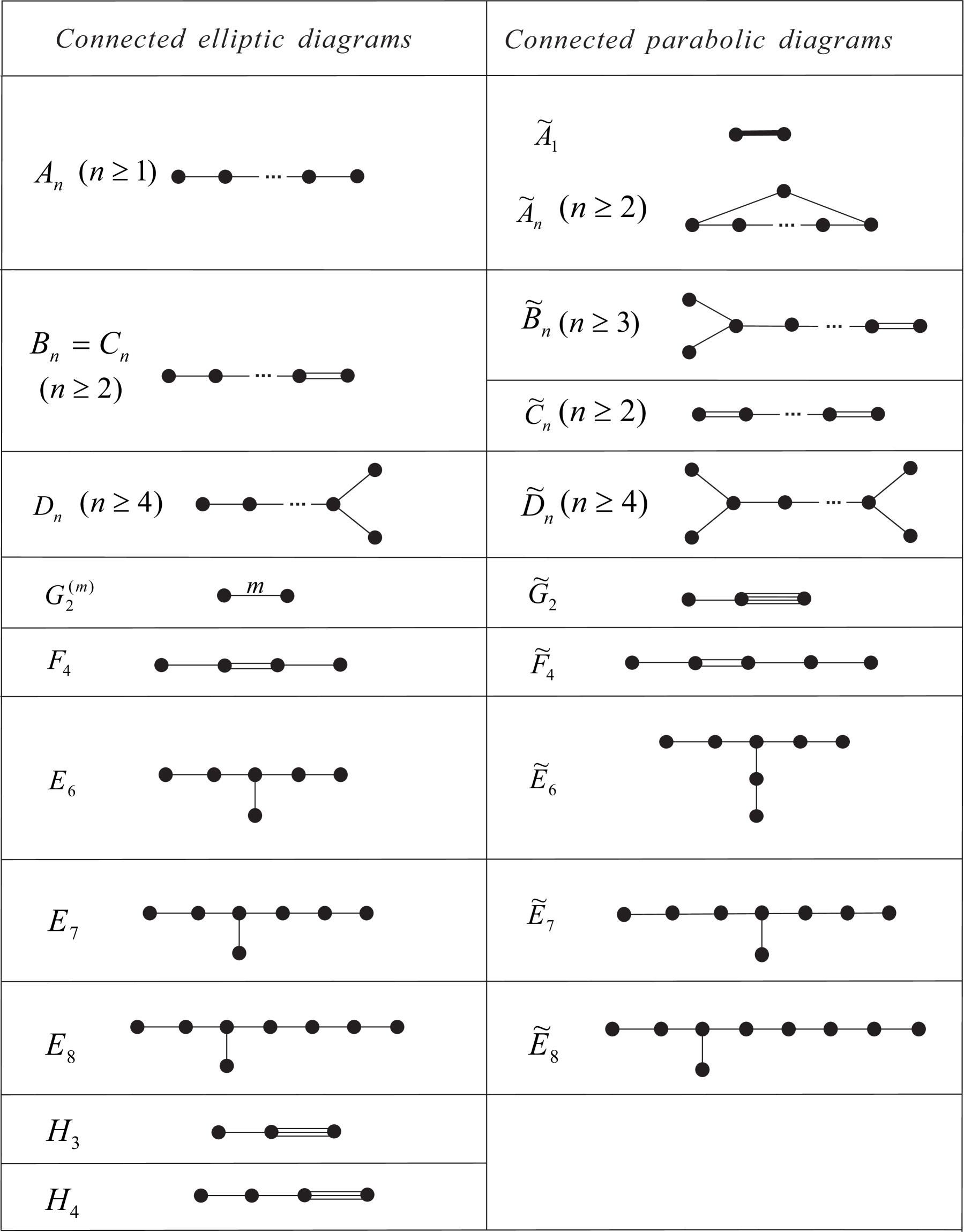
Figure 1. Connected elliptic (left) and connected parabolic (right) Coxeter diagrams.

In 1907, Perron found a remarkable property of eigenvalues and eigenvectors of matrices with positive entries. Frobenius later generalized it by investigating the spectral properties of indecomposable non-negative matrices.

Theorem 2.2 (Perron-Frobenius, [Gan59]).

An indecomposable real matrix $A=(a_{ij})$ with non-positive entries always possesses a unique positive eigenvalue $r$. The corresponding eigenvector exhibits all positive coordinates. The magnitudes of all other eigenvalues are not greater than $r$.

The Gram matrices $G(P)$ of an indecomposable Coxeter polytope are symmetric matrices with non-positive entries off the diagonal, and all diagonal elements are equal to $1$. By applying Theorem 2.2 to $I-G(P)$, where $I$ represents the identity matrix, we can identify a unique smallest eigenvalue of $G(P)$, denoted by $\lambda$. Depending on the value of $\lambda$, $G(P)$ can be classified as positive definite, semi-positive definite, or indefinite when $\lambda$ is greater than, equal to, or less than zero, respectively. In the case of being semi-definite, once again by utilizing Theorem 2.2, the deficiency of a connected semi-positive definite matrix $G(P)$ does not exceed $1$, and any proper submatrix of $G(P)$ is positive definite. For a Coxeter $n$-polytope $P$, its Coxeter diagram $\Sigma(P)$ is said to be elliptic if $G(P)$ is positive definite; $\Sigma(P)$ is called parabolic if any indecomposable component of $G(P)$ is degenerate and every subdiagram is elliptic. The elliptic and connected parabolic diagrams are proven to be the Coxeter diagrams of spherical and Euclidean Coxeter simplices, respectively. They are classified by Coxeter [Cox34] as shown in Figure 1.

A connected diagram $\Sigma$ is referred to as a Lannér diagram if it is neither elliptic nor parabolic, and every proper subdiagram of $\Sigma$ is elliptic. These diagrams represent irreducible Coxeter diagrams of compact hyperbolic Coxeter simplices. The complete list of such diagrams was initially reported by Lannér [Lan50], and the lists for $2$- and $3$-dimensional cases are provided in Figure 2. Similarly, non-compact hyperbolic simplices of finite volume can also be enumerated. The $2$- and $3$-dimensional lists of these simplices are presented in Figure 2 as well. They are characterized by connected Coxeter graphs known as quasi-Lannér diagrams, where proper subgraphs are either elliptic or connected parabolic.

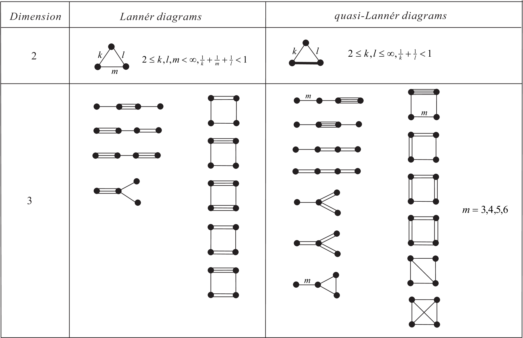
Figure 2. The Lannér and quasi-Lannér diagrams correspond to $2$- or $3$-dimensional hyperbolic Coxeter simplices, respectively.

Although the full list of hyperbolic Coxeter polytopes remains incomplete, some powerful algebraic restrictions are known [Vin$85^{(2)}$]:

Theorem 2.3.

([Vin$85^{(2)}$], Th. 2.1). Let $G=(g_{ij})$ be an indecomposable symmetric matrix of signature $(d,1)$, where $g_{ii}=1$ and $g_{ij}\leq 0$ if $i\neq j$. Then there exists a unique, up to isometry, convex hyperbolic polytope $P\subset\mathbb{H}^{d}$, whose Gram matrix coincides with $G$.

The counterpart theorem in the spherical and Euclidean settings is analogous, with the only difference being that the signature condition is revised to $(d+1,0)$ and $(d,0)$, respectively. This distinction also implies that we cannot expect a comparatively straightforward characterization of the potential combinatorial types of acute-angled polytopes in hyperbolic space.

Theorem 2.4.

([Vin$85^{(2)}$], Th. 3.1, Th. 3.2) Let $P=\mathop{\cap}\limits_{i\in I}H_{i}^{-}\in\mathbb{H}^{d}$ be an acute-angled polytope and $G=G(P)$ be the Gram matrix. Denote $G_{J}$ the principal submatrix of G formed from the rows and columns whose indices belong to $J\subset I$. Then,

1. The intersection $\mathop{\cap}\limits_{j\in J}H_{j}^{-}\in\mathbb{H}^{d},J\subset I$, is a face $F$ of $P$ if and only if the matrix $G_{J}$ is positive definite

2. The intersection $\overline{\mathop{\cap}\limits_{j\in J}H_{j}^{-}},J\subset I$, is an ideal vertex of $P$ if and only if the matrix $G_{J}$ is a parabolic matrix of rank $d-1$.

Theorem 2.5.

([Vin$85^{(2)}$], Th. 4.2) Let $P=\mathop{\cap}\limits_{i\in I}H_{i}^{-}\in\mathbb{H}^{d}$ be a convex polytope and $G=G(P)$ be its Gram matrix. Denote $G_{J}$ the principal submatrix of G formed from the rows and columns whose indices belong to $J\subset I$. Let $\mathcal{F}$ (resp. $\widetilde{\mathcal{F}}$) be the collection of elliptic submatrices $G_{J}$s (resp. elliptic and parabolic submatrices $G_{J}$s ). Partially order $\mathcal{F}$ (resp. $\widetilde{\mathcal{F}}$) by submatrix relation. Then, $P$ is compact (resp. finite-volume) if and only if any of the following conditions holds:

1. The polytope $P$ contains at least one ordinary vertex (resp. ordinary or ideal vertex). For every ordinary vertex (resp. vertex) of $P$ and any edge of $P$ emanating from it, there is precisely one other ordinary vertex (resp. vertex) of $P$ on that edge.

2. The partially ordered set $\mathcal{F}$ (resp. $\widetilde{\mathcal{F}}$) is isomorphic to the poset of some $d$-dimensional abstract combinatorial polytope.

Therefore, in order to classify all hyperbolic Coxeter $4$-polytopes with $7$ facets, we can begin by enumerating all Coxeter matrices of simple $4$-polytopes with $7$ facets that satisfy elliptic conditions around all ordinary vertices and parabolic conditions around all ideal vertices. Subsequently, we can further search for those with an indecomposable signature $(d,1)$ Gram matrix.

Last but not least, the volume of an even dimensional hyperbolic Coxeter polytope can be computed via its elliptic subgraphs. And we present some basic information here. Almost all the terminology and fact hold for general finitely generated groups, but we only state for finitely generated discrete reflection groups for our purpose.

Definition 2.6.

(Poincaré series) Let $\Gamma$ be a finitely generated group with a generating set $S$ corresponding to a $d$-dimensional hyperbolic polytope $P$. The Poincaré series of $\Gamma$ is the formal power series

$$f(\Gamma,S)=f_{S}(x)=\mathop{\Sigma}\limits_{g\in\Gamma}x^{l_{s}(g)},$$

where $l_{g}$ is the length function of $\Gamma$ with respect to S, i.e.

$$l_{g}(s)=min\{l\in\mathbb{N}~{}|~{}\exists s_{1},\cdots,s_{l}\in S\bigcup S^{-1}~{}\text{such that}~{}g=s_{1}s_{2}\cdots s_{l}\}.$$

Proposition 2.7.

([KP11]) Given a $d$-dimensional hyperbolic polytope $P$ where $d$ is even, and $\Gamma=\Gamma(P)$ is the corresponding finitely generated discrete reflection group, then

$$\text{volume}(P)=(-1)^{\frac{d}{2}}\cdot\frac{\pi^{\frac{d}{2}}\cdot 2^{d}\cdot\frac{d}{2}!}{d!}\cdot\chi(\Gamma),$$

where $\chi(\Gamma)$ is the orbifold Euler characteristic of the $\mathbb{H}/\Gamma$.

Moreover, let $\mathcal{E}=\{\Sigma^{{}^{\prime}}|\Sigma^{{}^{\prime}}\text{is an elliptic subgraphs of }\Sigma(P)\}$, and $\Gamma^{{}^{\prime}}$ the Coxeter subgroup corresponds to $\Sigma^{{}^{\prime}}$ , by Steinberg’s formula, we have

$$\chi(\Gamma)=\sum\limits_{\Sigma^{{}^{\prime}}\in\mathcal{E}}\frac{(-1)^{|\Sigma^{{}^{\prime}}|}}{f_{S^{{}^{\prime}}}(1)},$$

where $f_{S^{{}^{\prime}}}(1)$ is the value of Poincaré series at identity, i.e. the order of the subgroup $\Gamma^{{}^{\prime}}$, and $S^{{}^{\prime}}\subset S$ is the generating set of the subgroup of $\Gamma^{{}^{\prime}}$.

By means of the values in Table 1 [Gug17], it is straightforward to compute the hyperbolic volume of an even dimensional hyperbolic Coxeter polytope.

$A_{n}$	$B_{n}=C_{n}$	$D_{m}$	$G_{m}$	$F_{4}$	$E_{6}$	$E_{7}$	$E_{8}$	$H_{3}$	$H_{4}$
$(n+1)!$	$2^{n}\cdot n!$	$2^{n-1}\cdot n!$	$2n$	1,152	51,840	2,903,040	696,729,600	120	14,400

Table 1. Orders of finite Coxeter groups corresponding to elliptic diagrams.

3. Potential hyperbolic Coxeter matrices

Almost all of the terminologies and theorems in this section are proposed by Jacquemet and Tschantz and little adjustment might be adopted. We recall them here for reference, and readers can refer to [JT18] for more details.

3.1. Coxeter matrices

The Coxeter matrix of a hyperbolic Coxeter polytope $P$ is a symmetric matrix $M=(m_{ij})_{1\leq i,j\leq N}$ with entries in $\mathbb{N}\cup\{\infty\}$ such that

$$m_{ij}=\left\{\begin{array}[]{cl}1,&\text{if }j=i,\\ k_{ij},&\text{if }H_{i}\text{ and }H_{j}\text{ intersect in }\mathbb{H}^{n}\text{ with angle }\frac{\pi}{k_{ij}},~{}k_{ij}\in\mathbb{Z}_{\geq 2}\\ 0,&\text{if }H_{i}\text{ and }H_{j}\text{ intersect in }\partial\mathbb{H}^{n},\\ \infty,&\text{otherwise}.\end{array}\right.$$

Note that, compared with Gram matrix, the Coxeter matrix does not involve the specific information of the distances of the disjoint pairs.

Remark 3.1.

In the subsequent discussions, we refer to the Coxeter matrix $M$ of a graph $\Sigma$ as the Coxeter matrix $M$ of the Coxeter polyhedron $P$ such that $\Sigma=\Sigma(P)$.

3.2. Partial matrices

Definition 3.2.

Let $\Omega=\{n\in\mathbb{Z}\,|n=1~{}\text{or}~{}\,n\geq 2\}\cup\{\infty\}$ and let $\bigstar$ be a symbol representing an undetermined real value. A partial matrix of size $m\geq 1$ is a symmetric $m\times m$ matrix $M$ whose diagonal entries are $1$, and whose non-diagonal entries belong to $\Omega\cup\{\bigstar\}$.

Definition 3.3.

Let $M$ be an arbitrary $m\times m$ matrix, and $s=(s_{1},s_{2},\cdots,s_{k})$, $1\leq s_{1}<s_{2}<\cdots<s_{k}\leq m$. Let $M^{s}$ be the $k\times k$ submatrix of $M$ with $(i,j)$-entry $m_{s_{i},s_{j}}$.

Definition 3.4.

We say that a partial matrix $M=(p_{ij})_{1\leq i,j,\leq m}$ is a potential matrix for a given polytope $P$ if

$\bullet$ There are no entries with the value $\bigstar$;

$\bullet$ There are entries $\infty$ in positions of $M$ that correspond to disjoint pair;

$\bullet$ For every sequence $s$ of indices of facets meeting at an ordinary vertex $v$ of $P$, the matrix, obtained by replacing value $k_{ij}$ with $-\cos\frac{\pi}{k_{ij}}$ of submatrix $M^{s}$, is elliptic; For every sequence $s$ of indices of facets meeting at an ideal vertex $v$ of $P$, the matrix, obtained by replacing value $k_{ij}$ with $-\cos\frac{\pi}{k_{ij}}$ and value $0$ with $-1$ of submatrix $M^{s}$, is parabolic.

For brevity, we use a potential vector

$$C=(p_{12},p_{13},\cdots p_{1m},p_{23},p_{24},\cdots,p_{2m},\cdots p_{ij},\cdots p_{m-1,m}),~{}p_{ij}\neq\infty$$

to denote the potential matrix, where $1\leq i<j\leq m$ and non-infinity entries are placed by the subscripts lexicographically. The potential matrix and potential vector $C$ can be constructed one from each other easily. In general, an arbitrary Coxeter matrix corresponds to a Coxeter vector following the same manner. We mainly use the language of vectors to explain the methodology and report the enumeration results. It is worth remarking that for a given Coxeter diagram, the corresponding (potential / Gram) matrix and vector are not unique in the sense that they are determined under a given labeling system of the facets and may vary when the system changes. In Section 5, we apply a permutation group to the nodes of the diagram and remove the duplicates to obtain all of the distinct desired vectors

For each rank $r\geq 2$, there are infinitely many finite Coxeter groups, because of the infinite 1-parameter family of all dihedral groups, whose graphs consist of two nodes joined by an edge of weight $k\geq 2$. However, a simple but useful truncation can be utilized:

Proposition 3.5.

There are finitely many finite Coxeter groups of rank $r$ with Coxeter matrix entries at most seven.

We remark that in order to minimize the number of angle variables involved in the second phase of the signature obstruction computation in Mathematica, we have deliberately selected the integer $7$ instead of any smaller value. The weights larger than or equal to $6$ only show up in the case of $G_{2}^{m}$ and the weight $6$ with an entry of $\cos\frac{\pi}{6}=\frac{1}{2}$ in the Gram matrix remains computationally straightforward. Hence, we move the bound one up to $7$. Theoretically, the bound can be an arbitrary integer larger than or equal to $2$. However, the smaller the bound is, the more angle variables will be added in the minor equations claimed in Section 6; whilst the larger the bound is, the bigger the pre-block $\mathcal{S}^{*}$, which is defined in the block-pasting algorithm in Section 5, will be. For example, if the bound is $8$, many more vectors, like $(2,2,2,2,2,8),(2,2,2,2,8,2),(2,2,3,8,2,2),\cdots$ , will be added to $\mathcal{S}$, which is unexpected in the programming for the pre-block is repeatedly used in the algorithm whenever a new vertex is covered, and will therefore increase the computation load greatly. The number $7$ turns out to be the optimal choice.

It thus suffices to enumerate potential matrices with entries at most seven, and the other candidates can be obtained from substituting integers greater than seven with the value seven. In other words, we now have more variables, that are restricted to be integers larger than or equal to seven, besides length unknowns. In the following, we always use the terms “Coxeter matrix” or “potential matrix” to mean the one with integer entries less than or equal to seven unless otherwise mentioned.

In [JT18], the problem of finding certain hyperbolic Coxeter polytopes is solved in two phases. In the first step, potential matrices for a particular hyperbolic Coxeter polytope are found; the “Euclidean-square obstruction” is used to reduce the number. Secondly, relevant algebraic conditions are solved for the admissible distances between non-adjacent facets. In our setting, additional universal necessary conditions, except for the vertex spherical restriction and Euclidean square obstruction, are adopted and programmed to reduce the number of the potential matrices.

4. combinatorial type of simple 4-polytopes with 7 facets

The classification of combinatorial types of $d$-polytopes with $m$ facets for $m\leq d+3$ was achieved by using Gale diagrams. For simple $d$-polytopes with $m$ facets, there is a formula by Perles, see for example [Grü67], and also [BD98]. We learn the following data of simple $4$-polytopes with $7$ facets from the website

https://www-imai.is.s.u-tokyo.ac.jp/$\sim$hmiyata/oriented_matroids/index.html

by Hiroyuki Miyata, where the number $0$, $1$, $\cdots$, $6$ denote the seven facets, and each line of the file contains exactly one face lattice represented by the list of vertice and each bracket corresponds to a vertex. For example, there are $9$ vertices of the above polytope $P_{1}$. Additionally, the first vertex is contained in six facets. We call each bracket a facet bracket corresponding to some vertex.

label	admissible	facet brackets
1	$P_{1}$	[6,5,4,3,2,1] [6,5,4,0] [6,5,3,0] [6,4,2,0] [6,3,2,0] [5,4,1,0] [5,3,1,0] [4,2,1,0] [3,2,1,0]
2		[6,5,4,3,2,1] [6,5,4,0] [6,5,3,0] [6,4,3,0] [5,4,2,0] [5,3,2,0] [4,3,1,0] [4,2,1,0] [3,2,1,0]
3		[6,5,4,3,2,1] [6,5,4,3,0] [6,5,2,0] [6,4,2,0] [5,3,1,0] [5,2,1,0] [4,3,1,0] [4,2,1,0]
4		[6,5,4,3,2,1] [6,5,4,3,0] [6,5,2,0] [6,4,2,0] [5,3,2,0] [4,3,1,0] [4,2,1,0] [3,2,1,0]
5		[6,5,4,3,2,1] [6,5,4,3,0] [6,5,2,1,0] [4,3,2,1,0] [6,4,2,0] [5,3,1,0]
6		[6,5,4,3,2,1] [6,5,4,3,0] [6,5,2,1,0] [6,4,2,0] [5,3,1,0] [4,3,2,0] [3,2,1,0]
7		[6,5,4,3,2,1] [6,5,4,3,2,0] [6,5,1,0] [6,4,1,0] [5,3,1,0] [4,2,1,0] [3,2,1,0]
8	$P_{2}$	[6,5,4,3,2] [6,5,4,1,0] [6,3,2,1,0] [6,5,3,1] [6,4,2,0] [5,4,3,1] [4,3,2,1] [4,2,1,0]
9	$P_{3}$	[6,5,4,3,2] [6,5,4,1,0] [6,5,3,1] [6,4,3,0] [6,3,1,0] [5,4,2,1] [5,3,2,1] [4,3,2,0] [4,2,1,0] [3,2,1,0]
10	$P_{4}$	[6,5,4,3,2] [6,5,4,1,0] [6,5,3,1] [6,4,3,0] [6,3,1,0] [5,4,2,1] [5,3,2,1] [4,3,2,1] [4,3,1,0]
11	$P_{5}$	[6,5,4,3,2] [6,5,4,1,0] [6,5,3,1] [6,4,3,1] [5,4,2,0] [5,3,2,1] [5,2,1,0] [4,3,2,0] [4,3,1,0] [3,2,1,0]
12	$P_{6}$	[6,5,4,3,2] [6,5,4,1,0] [6,5,3,1] [6,4,3,1] [5,4,2,0] [5,3,2,1] [5,2,1,0] [4,3,2,1] [4,2,1,0]
13	$P_{7}$	[6,5,4,3,2] [6,5,4,1] [6,5,3,1] [6,4,3,0] [6,4,1,0] [6,3,1,0] [5,4,2,1] [5,3,2,0] [5,3,1,0] [5,2,1,0] [4,3,2,0] [4,2,1,0]
14	$P_{8}$	[6,5,4,3,2] [6,5,4,1] [6,5,3,1] [6,4,3,0] [6,4,1,0] [6,3,1,0] [5,4,2,1] [5,3,2,1] [4,3,2,0] [4,2,1,0] [3,2,1,0]
15	$P_{9}$	[6,5,4,3,2] [6,5,4,1] [6,5,3,1] [6,4,3,1] [5,4,2,0] [5,4,1,0] [5,3,2,0] [5,3,1,0] [4,3,2,0] [4,3,1,0]
16	$P_{10}$	[6,5,4,3,2] [6,5,4,1] [6,5,3,1] [6,4,3,1] [5,4,2,1] [5,3,2,0] [5,3,1,0] [5,2,1,0] [4,3,2,0] [4,3,1,0] [4,2,1,0]
17	$P_{11}$	[6,5,4,3,2] [6,5,4,1] [6,5,3,1] [6,4,3,1] [5,4,2,1] [5,3,2,1] [4,3,2,0] [4,3,1,0] [4,2,1,0] [3,2,1,0]
18		[6,5,4,3,2] [6,5,4,3,1] [6,5,2,0] [6,5,1,0] [6,4,2,0] [6,4,1,0] [5,3,2,0] [5,3,1,0] [4,3,2,0] [4,3,1,0]
19		[6,5,4,3,2] [6,5,4,3,1] [6,5,2,1,0] [4,3,2,1,0] [6,4,2,1] [5,3,2,0] [5,3,1,0]
20		[6,5,4,3,2] [6,5,4,3,1] [6,5,2,1,0] [6,4,2,0] [6,4,1,0] [5,3,2,0] [5,3,1,0] [4,3,2,0] [4,3,1,0]
21		[6,5,4,3,2] [6,5,4,3,1] [6,5,2,1,0] [6,4,2,1,0] [5,3,2,0] [5,3,1,0] [4,3,2,0] [4,3,1,0]
22		[6,5,4,3,2] [6,5,4,3,1] [6,5,2,1,0] [6,4,2,1] [5,3,2,0] [5,3,1,0] [4,3,2,0] [4,3,1,0] [4,2,1,0]
23		[6,5,4,3,2] [6,5,4,3,1] [6,5,2,1,0] [6,4,2,1] [5,3,2,0] [5,3,1,0] [4,3,2,1] [3,2,1,0]
24		[6,5,4,3,2] [6,5,4,3,1] [6,5,2,1] [6,4,2,0] [6,4,1,0] [6,2,1,0] [5,3,2,0] [5,3,1,0] [5,2,1,0] [4,3,2,0] [4,3,1,0]
25		[6,5,4,3,2] [6,5,4,3,1] [6,5,2,1] [6,4,2,1] [5,3,2,0] [5,3,1,0] [5,2,1,0] [4,3,2,0] [4,3,1,0] [4,2,1,0]
26		[6,5,4,3,2] [6,5,4,3,1] [6,5,2,1] [6,4,2,1] [5,3,2,1] [4,3,2,0] [4,3,1,0] [4,2,1,0] [3,2,1,0]
27	$P_{12}$	[6,5,4,3] [6,5,4,2] [6,5,3,2] [6,4,3,1] [6,4,2,1] [6,3,2,0] [6,3,1,0] [6,2,1,0] [5,4,3,1] [5,4,2,0] [5,4,1,0] [5,3,2,0] [5,3,1,0] [4,2,1,0]
28	$P_{13}$	[6,5,4,3] [6,5,4,2] [6,5,3,2] [6,4,3,1] [6,4,2,1] [6,3,2,1] [5,4,3,0] [5,4,2,0] [5,3,2,0] [4,3,1,0] [4,2,1,0] [3,2,1,0]
29	$P_{14}$	[6,5,4,3] [6,5,4,2] [6,5,3,2] [6,4,3,1] [6,4,2,1] [6,3,2,1] [5,4,3,1] [5,4,2,0] [5,4,1,0] [5,3,2,0] [5,3,1,0] [4,2,1,0] [3,2,1,0]
30	$P_{15}$	[6,5,4,3] [6,5,4,2] [6,5,3,2] [6,4,3,2] [5,4,3,1] [5,4,2,1] [5,3,2,0] [5,3,1,0] [5,2,1,0] [4,3,2,0] [4,3,1,0] [4,2,1,0]
31	$P_{16}$	[6,5,4,3] [6,5,4,2] [6,5,3,2] [6,4,3,2] [5,4,3,1] [5,4,2,1] [5,3,2,1] [4,3,2,0] [4,3,1,0] [4,2,1,0] [3,2,1,0]

Table 2. Out of the 31 4-dimensional polytopes with 7 facets, there are 16 admissible polytopes that can potentially be realized as combinatorial types of Coxeter hyperbolic polytopes. Note that the polytope $P_{1}$ is the only pyramid in this family which is a pyramid over the product of three $1$-simplices.

Furthermore, among the total of 31 polytopes, our focus will be exclusively on the $16$ admissible ones whose vertex links are either $3$-simplices, $3$-dimensional simplicial prisms, or $3$-cubes. The vertex link of an ideal vertex $v_{\infty}$ is determined by the intersection of the polytope $P$ with a sufficiently small horosphere centered at $v_{\infty}$. This horosphere should not intersect any facet of $P$ that is not incident to $v_{\infty}$.

The subgraphs formed by nodes that correspond to facets intersecting at ideal points yield parabolic graphs, which represent $3$-dimensional Euclidean Coxeter polytopes. In particular, the vertex whose vertex figure is a $3$-dimensional simplicial prism corresponds to a bracket with $5$ entries, where the disjoint pair of $2$ facets is colored green; the vertex whose vertex figure is a $3$-dimensional cube corresponds to a bracket with $6$ entries, where the disjoint two pairs are colored green and pink, respectively.

Now, let us exemplify the process of selecting the 16 polyhedra that meet the given criteria as follows:

1. The 4-dimensional polytope with seven facets can be realized as a cone over a 3-dimensional polytope with six facets. To ensure that the vertex link satisfies the requirement of being a simple 3-dimensional polytope, where exactly three facets intersect at each vertex, we impose certain conditions. Specifically, we allow only one vertex’s vertex link to be a 3-cube, while the vertex links of other vertices must be 3-simplices. Additionally, the number of vertices in the vertex link of the 3-simplex must be equal to the number of vertices in the 3-dimensional cube, which is 8. Consequently, out of the first 7 combinations with a bracket length of 6, only the first two combinations meet the specified requirements. Moreover, it is evident that only the first combination represents a cone over a 3-cube.
   

2. For a vertex formed by the intersection of five faces, we can determine its vertex link lattice through a straightforward combination calculation. Specifically, we identify the set of vertices whose facet brackets intersect with the facet bracket of the vertex, having a length of five, at exactly three common entries. This set then serves as the candidate vertex links, which are subsequently compared against the 3-prism. By conducting this comparison, we can effectively identify and exclude vertex links that do not represent cones over 2-cubes but rather 3-prisms.

Furthermore, based on the combinatorial information in Table 2, we can derive the following (1)–(7) data for each admissible polytope. To illustrate, we provide an example of the data for $P_{11}$ in Table 3.

1. The set $d_{k}$ consists of pairs of facets that are disjoint.

2. The set $l_{3}$ or $l_{4}$ comprises sets of three or four facets, where the intersections exhibit the combinatorial structure of a triangle or a tetrahedron.

3. The set $s_{3}$ comprises sets of three facets, where the intersection is not an edge of $P_{k}$, and no disjoint pairs are included.

4. The set $e_{3}$ consists of sets of three facets of $P_{k}$ from which the triples in ideal vertices corresponding to Euclidean triangles are excluded, and no disjoint pairs are included.

5. The set $s_{4}=e_{4}$ consists of sets of four facets, where the intersections are not vertices of $P_{k}$. It excludes the tetrads in ideal vertices corresponding to Euclidean cubes and does not include any disjoint pairs.

6. The set $s_{5}$ or $s_{6}$ comprises sets of five or six facets, where no disjoint pairs are included.

7. The set $e_{5}$ or $e_{6}$ consists of sets of five or six facets, excluding the 5-tuples or 6-tuples corresponding to ideal vertices with vertex links of $3$-prisms or $3$-cubes. Additionally, no disjoint pairs are included.

$P_{11}$
Vert	10	$\{\{{\color[rgb]{0,1,0}6},5,4,3,{\color[rgb]{0,1,0}2}\},\{6,5,4,1\},\{6,5,3,1\},\{6,4,3,1\},\{5,4,2,1\},\{5,3,2,1\},\{4,3,2,0\},\{4,3,1,0\},\{4,2,1,0\},\{3,2,1,0\}\}$
$d_{11}$	2	$\{\{0,5\},\{0,6\}\}$
$l_{3}$	0	$\{\}$
$l_{4}$	1	$\{\{1,2,3,4\}\}$
$s_{3}$	5	$\{\{1,2,6\},\{2,3,6\},\{2,4,6\},\{2,5,6\},\{3,4,5\}\}$
$e_{3}$	$25$	$\{\{0,1,2\},\{0,1,3\},\{0,1,4\},\{0,2,3\},\{0,2,4\},\{0,3,4\},\{1,2,3\},\{1,2,4\},\{1,2,5\},\{1,2,6\},\{1,3,4\},\{1,3,5\}$
		$\{1,3,6\},\{1,4,5\},\{1,4,6\},\{1,5,6\},\{2,3,4\},\{2,3,5\},\{2,3,6\},\{2,4,5\},\{2,4,6\},\{2,5,6\},\{3,4,6\},\{3,5,6\},$
		$\{4,5,6\}\}$
$s_{4}=e_{4}$	$7$	$\{\{1,2,3,4\},\{1,2,3,6\},\{1,2,4,6\},\{1,2,5,6\},\{1,3,4,5\},\{2,3,4,5\},\{3,4,5,6\}\}$
$s_{5}$	7	$\{\{0,1,2,3,4\},\{1,2,3,4,5\},\{1,2,3,4,6\},\{1,2,3,5,6\},\{1,2,4,5,6\},\{1,3,4,5,6\},\{2,3,4,5,6\}\}$
$e_{5}$	6	$\{\{0,1,2,3,4\},\{1,2,3,4,5\},\{1,2,3,4,6\},\{1,2,3,5,6\},\{1,2,4,5,6\},\{1,3,4,5,6\}\}$
$s_{6}$	1	$\{\{1,2,3,4,5,6\}\}$
$e_{6}$	1	$\{\{1,2,3,4,5,6\}\}$

Table 3. Combinatorics of the combinatorial polytope $P_{11}$.

5. Block-pasting algorithms for enumerating all the candidate matrices over certain combinatorial types.

We now use the block-pasting algorithm to determine all of the potential matrices for the $16$ combinatorial types reported in Section 4. Recall that the entries have only finite options, i.e., $k_{ij}\in\{0,1,2,3,\cdots,7\}\cup\{\infty\}$. Compared to the backtracking search algorithm raised in [JT18], “block-pasting” algorithm is more efficient and universal. Generally speaking, the backtracking search algorithm uses the method of “a series circuit”, where the potential matrices are produced one by one. Whereas, the block-pasting algorithm adopts the idea of “a parallel circuit”, where different parts of a potential matrix are generated simultaneously and then pasted together.

For each vertex $v_{i}$ of a 4-dimensional hyperbolic Coxeter polytope $P_{k}$, we define a “chunk” $k_{i}$ consists of an ordered set of facets that intersect at vertex $v_{i}$ with the subscripts in ascending order. The chunk is called “ordinary” or “ideal” if the vertex is ordinary or ideal. For example, for the polytope $P_{1}$ discussed above, there are $8$ ordinary chunks and $1$ ideal chunk as it has $8$ simple vertices and $1$ non-simple vertex with the vertex link a 3-cube. We may also use $k_{i}$ to denote the ordered set of subscripts, i.e., $k_{i}$ is referred to as a set of integers of length four, five or six.

Since the vertex links of finite-volume hyperbolic $4$-dimensional polytopes are either simplex, simplicial 3-prism or 3-cube, each chunk possesses $6$, $9$, or $12$ dihedral angles. For every chunk $k_{i}$, we define an i-label set $e_{i}$ to be the ordered set $\{10a+b~{}|~{}\{a,b\}\in E_{i}\}$, where $E_{i}$, named the i-index set, is the ordered set of labels of non-parallel pairs of facets and sorted lexicographically. For example, For the polytope $P_{7}$ shown in Table 2, the facets $F_{6}$, $F_{5}$, $F_{4}$, $F_{3}$, and $F_{2}$ intersect at the first ideal vertex with vertex link a $3$-dimensional prism, where $F_{6}$ and $F_{2}$ are parallel. Then, we have

$$k_{1}=\{F_{2},F_{3},F_{4},F_{5},F_{6}\}~{}(\text{or}~{}\{2,3,4,5,6\}),$$

$$E_{1}=\{\{2,3\},\{2,4\},\{2,5\},\{3,4\},\{3,5\},\{3,6\},\{4,5\},\{4,6\},\{5,6\}\},$$

$$e_{1}=\{23,24,25,34,35,36,45,46,56\}.$$

Next, we list all of the Coxeter vectors of rank $4$ elliptic Coxeter diagrams and rank $4$ parabolic Coxeter diagrams with $4$, $5$, or $6$ nodes as shown in Figure 3. Note that the finiteness of the diagrams is a result of our convention to consider only those diagrams with integer weights less than or equal to seven.

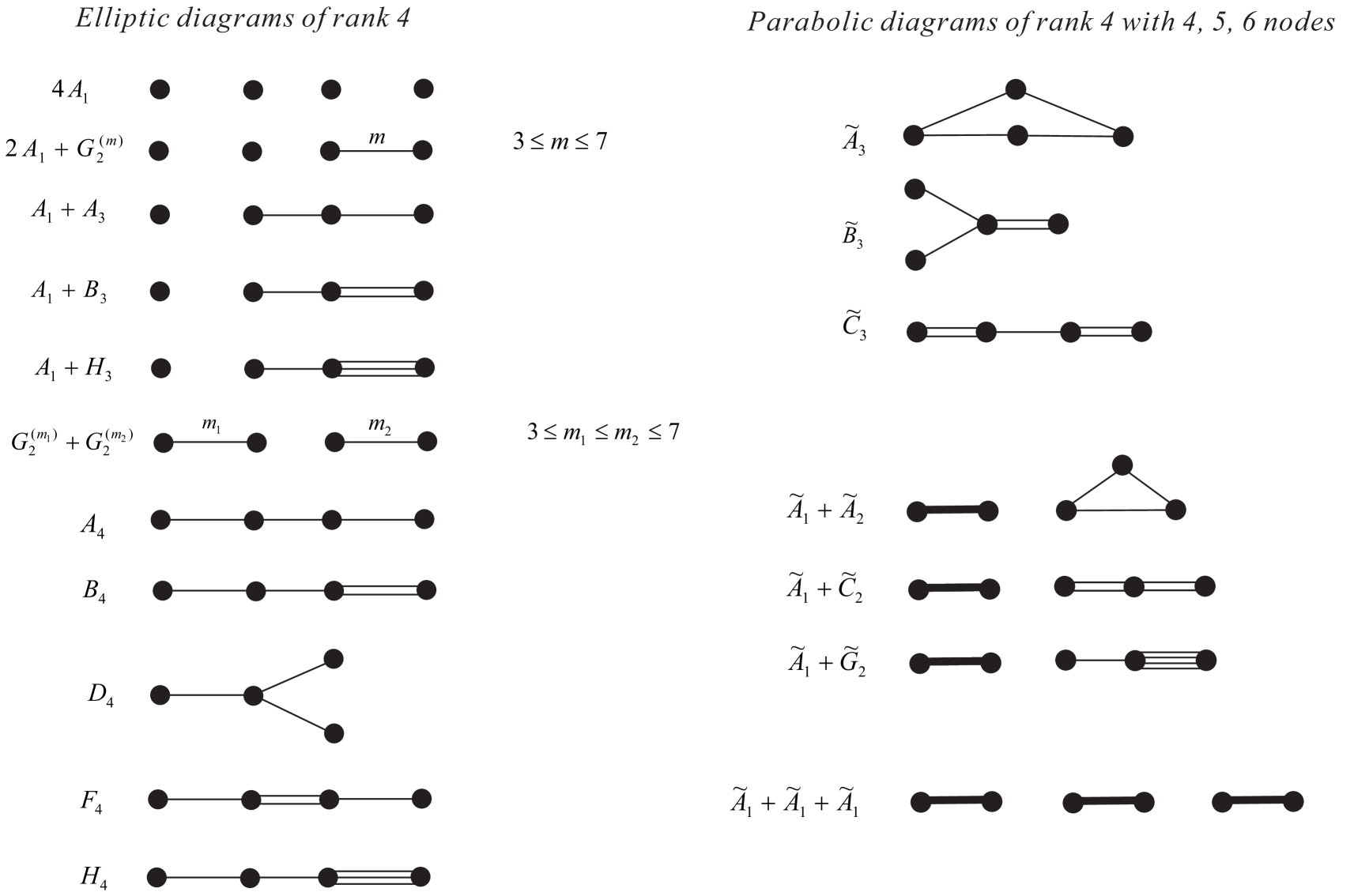
Figure 3. Spherical Coxeter diagrams of rank $4$ and parabolic Coxeter diagram of rank $4$ with nodes $4$, $5$, and $6$. Only diagrams with integer entries less than or equal to seven are under consideration.

We apply permutation groups on four, five, and six letters, denoted by $S_{4}$, $S_{5}$, and $S_{6}$ respectively, to the labels of the nodes in the Coxeter diagrams shown in Figure 3. This process generates all possible vectors by varying the order of the facets. For instance, there are four vectors associated with the single diagram $D_{4}$, as depicted in Figure 4. The Coxeter diagrams in Figure 3 yield $269$, $10$, and $1$ distinct vectors corresponding to the order $4$, $5$, and $6$ of diagrams respectively. These vectors are then arranged into sets $\mathcal{S}^{4}$, $\mathcal{S}^{5}$, and $\mathcal{S}^{6}$, referred to as the $4$-preblock, $5$-preblock, and $6$-preblock respectively. These sets can be represented as $269\times 6$, $10\times 9$, and $1\times 12$ matrices in a straightforward manner. In the following, we do not differentiate between these two perspectives and may refer to $\mathcal{S}^{*}$, where $*=4,5,6$, as either a set or a matrix depending on the context.

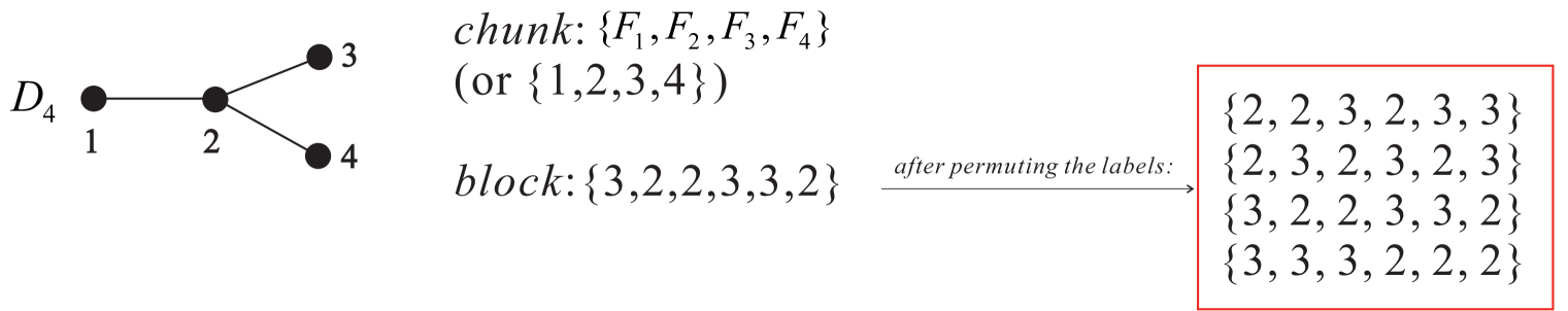
Figure 4. prepare the pre-block

We proceed by generating a dataframe $B_{i}$, referred to as the $i$-block, for each chunk $k_{i}$ of a given polytope $P_{k}$, where $1\leq i\leq|V_{k}|$ and $|V_{k}|$ is the number of vertices of $P_{k}$. Note that the size of the dataframe depends on whether the vertex link corresponds to a $3$-simplex, a $3$-dimensional prism, or a $3$-dimensional cube, of which the dataframe will be of size $269\times 6$, $10\times 9$, or $1\times 12$ accordingly.

Firstly we evaluate $B_{i}$ by suitable $\mathcal{S}^{*}$ and take the ordered set $e_{i}$ defined above as the column names of $B_{i}$. For example, for $e_{1}=\{12,14,15,24,25,45\}$, the columns of $B_{i}$ are referred to as $(12)$-, $(14)$-, $(15)$-, $(24)$-, $(25)$-, $(45)$-columns.

For each admissible polytopes $P_{k}$, the set of disjoint pairs of facets, denoted by $d_{k}$ is shown in Table 4. We may also use $d_{k}$ to represent the label set $\{10a+b~{}|~{}{a,b}\in d_{k}\}$ if there is no ambiguity.

$P_{k}$	1	2	3	4	6	8	9	11	16
Disjoint pairs $d_{k}$	{}	{}	{}	{{0,2}}	{{0,3}}	{{0,5}}	{{0,6},{1,2}}	{{0,5},{0,6}}	{{0,5},{0,6},{1,6}}
	5	7	12	10	14		13	15
	{}	{}	{}	{{0,6}}	{{0,6}}		{{1,5},{0,6}}	{{0,6},{1,6}}

Table 4. The set $d_{k}$ of disjoint pairs of facets for each admissible polytope $P_{k}$.

Denote $L$ to be a vector of length $21$ as follows:

$$L=\{01,02,03,...,06{\color[rgb]{1,0,0},}~{}12,13,...,16{\color[rgb]{1,0,0},}~{}23,24,...,26{\color[rgb]{1,0,0},}~{}34,35,36{\color[rgb]{1,0,0},}~{}45,46{\color[rgb]{1,0,0},}~{}56\}.$$

Next, we extend each $269\times 6$, $10\times 9$, or $1\times 12$ dataframe to a $k\times 21$ dataframe, where $k=269,~{}9,~{}1$, with column names denoted by $L$. This is done by placing each $(ij)$-column in the corresponding labeled column position, filling in the symbol of infinity for the $(ij)$-columns where $ij\in d_{k}$, and filling in the value zero for the remaining positions. We continue to use the same notation $B_{i}$ for the extended dataframe.

For example, for the polytope $P_{8}$, the set $d_{8}=\{05\}$ and the vertex link of the first ideal vertex is a $3$-prism with a pair of parallel facets $\{2,6\}$ as shown in Table 2. Then we have the $B_{1}$ of $P_{8}$ as follows:

	01	02	03	04	05	06	12	13	14	15	16	23	24	25	26	34	35	36	45	46	56
1	*	*	*	*	$\infty$	*	*	*	*	*	*	2	2	2	0	6	3	2	2	2	2
2	*	*	*	*	$\infty$	*	*	*	*	*	*	2	2	2	0	4	4	2	2	2	2
3	*	*	*	*	$\infty$	*	*	*	*	*	*	2	2	2	0	3	6	2	2	2	2
4	*	*	*	*	$\infty$	*	*	*	*	*	*	2	2	2	0	6	2	2	3	2	2
5	*	*	*	*	$\infty$	*	*	*	*	*	*	2	2	2	0	3	3	2	3	2	2
6	*	*	*	*	$\infty$	*	*	*	*	*	*	2	2	2	0	2	6	2	3	2	2
7	*	*	*	*	$\infty$	*	*	*	*	*	*	2	2	2	0	4	2	2	4	2	2
8	*	*	*	*	$\infty$	*	*	*	*	*	*	2	2	2	0	2	4	2	4	2	2
9	*	*	*	*	$\infty$	*	*	*	*	*	*	2	2	2	0	3	2	2	6	2	2
10	*	*	*	*	$\infty$	*	*	*	*	*	*	2	2	2	0	2	3	2	6	2	2

Table 5. The first block $B_{1}$ of the polytope $P_{8}$.

After preparing all of the blocks $B_{i}$ for a given polytope $P_{k}$, we proceed to paste them up. More precisely, when pasting $B_{1}$ and $B_{2}$, a row from $B_{1}$ is matched up with a row of $B_{2}$ where every two entries specified by the same index $i$, where $i\in e_{1}\cap e_{2}$, have the same values. The index set $e_{1}\cap e_{2}$ is called a linking key for the pasting. The resulting new row is actually the sum of these two rows in the non-key positions; the values are retained in the key positions. The dataframe of the new data is denoted by $B_{1}\cup^{*}B_{2}$.

We use the following example to explain this process. Suppose

$B_{1}=\{x_{1},x_{2}\}=\{(2,2,3,2,3,4,\infty,*,*,*\cdots,*),(2,3,4,4,2,2,\infty,*,*,*,\cdots,*)\}$,

$B_{2}=\{y_{1},y_{2},y_{3}\}=\{(2,2,3,2,*,*,\infty,4,3,*,\cdots,*),(2,3,4,4,*,*,\infty,2,2,*,\cdots,*)$,

$(3,3,2,2,*,*,\infty,3,3,*,\cdots,*)\}.$

In this example, $x_{1}$ and $x_{2}$ have the same values with $y_{1}$ and $y_{2}$ on the $(01)$-, $(02)$-, $(03)$- and $(04)$- positions, respectively. In other words, the linking key here is $\{01,02,03,04\}$. Thus, $y_{1}$ and $y_{2}$ can paste to $x_{1}$ and $x_{2}$, respectively to form the Coxeter vectors

$$(2,2,3,2,3,4,\infty,4,3,*,\cdots,*)~{}\text{and}~{}(2,3,4,4,2,2,\infty,2,2,*,\cdots,*),\text{respectively}.$$

In contrast, $y_{3}$ cannot be pasted to any element of $B_{1}$ as there are no vectors with entry $3$ on the $(01)$-position. Therefore,

$$B_{1}\cup^{*}B_{2}=\{(2,2,3,2,3,4,\infty,4,3,*,\cdots,*),(2,3,4,4,2,2,\infty,2,2,*,\cdots,*)\}.$$

We then move on to paste the sets $B_{1}\cup^{*}B_{2}$ and $B_{3}$. We follow the same procedure with an updated index set. The linking key is now $e_{1}\cup e_{2}\cap e_{3}$. We conduct this procedure until we finish pasting the final set $B_{|V_{k}|}$. The set of linking keys used in this procedure is

$$\{e_{1}\cap e_{2},e_{1}\cup e_{2}\cap e_{3},\cdots,e_{1}\cup e_{2}\cup\cdots\cup e_{i-1}\cap e_{i},\cdots,e_{1}\cup e_{2}\cup\cdots\cup e_{|V|-1}\cap e_{|V|}\}.$$

During the process of pasting, in order to manage the peak volume of resulting vectors and ensure computational feasibility, we have imposed additional restrictions to refine the program. The refined approach aims to introduce additional necessary conditions, apart from the vertex elliptic or parabolic restriction, with the objective of reducing the number of vectors involved in the block-pasting process.

Firstly, we collect data sets $\mathcal{L}_{3}$, $\mathcal{L}_{4}$, $\mathcal{S}_{3}$, $\mathcal{S}_{4}$, $\mathcal{S}_{5}$, $\mathcal{S}_{6}$, $\mathcal{E}_{3}$, $\mathcal{E}_{4}$, $\mathcal{E}_{5}$, and $\mathcal{E}_{6}$ as claimed in Table 6, by the following two steps:

1. Prepare Coxeter diagrams with the appropriate rank and node as described in Table 6, and record the Coxeter vectors using an arbitrary system of node labeling.

2. Apply the permutation group $S_{n}$ to the node labels and generate the desired dataset, which includes all distinct Coxeter vectors obtained from different labeling systems.

Types of Coxeter diagrams	# Coxeter diagrams	# distinct Coxeter	data sets
		Vectors after
		permutation on nodes
Coxeter diagrams of hyperbolic $2$-simplices	44 (Lannér)	280	$\mathcal{L}_{3}$
with weights no more than 7	20 ( quasi-Lannér)
Coxeter diagrams of hyperbolic 3-simplices	9 (Lannér)	368	$\mathcal{L}_{4}$
	21 (quasi-Lannér)
rank $3$ elliptic Coxeter diagrams	9	31	$\mathcal{S}_{3}$
rank $4$ elliptic Coxeter diagrams	29	242	$\mathcal{S}_{4}$
rank $5$ elliptic Coxeter diagrams	47	1946	$\mathcal{S}_{5}$
rank $6$ elliptic Coxeter diagrams	117	20206	$\mathcal{S}_{6}$
parabolic Coxeter diagrams with 3 nodes (rank 2)	3	10	$\mathcal{E}_{3}$
parabolic parabolic Coxeter diagrams with 4 nodes (rank 2 or 3)	4	30	$\mathcal{E}_{4}$
parabolic parabolic Coxeter diagrams with 5 nodes (rank 2 or 3)	8	357	$\mathcal{E}_{5}$
parabolic Coxeter diagrams with node 6 (rank 3, 4, or 5)	14	2290	$\mathcal{E}_{6}$

Table 6. Data sets used to reduce the computational load.

Next, we modify the block-pasting algorithm by using additional metric restrictions. More precisely, remarks 5.1–5.3, which are practically reformulated from Theorem 2.4, must be satisfied.

Remark 5.1.

(“(quasi-)Lannér-condition”) The Coxeter vector of the three/six dihedral angles formed by the three/four facets with the labels indicated by the data in $l_{3}$/$l_{4}$ is IN $\mathcal{L}_{3}$/$\mathcal{L}_{4}$.

Remark 5.2.

(“spherical-condition”) The Coxeter vector of the three/six/ten/fifteen dihedral angles formed by the three/four/five/six facets with the labels indicated by the data in $s_{3}$/$s_{4}$/$se_{5}$/$se_{6}$ is NOT IN $\mathcal{S}_{3}$/$\mathcal{S}_{4}$/$\mathcal{S}_{5}$/$\mathcal{S}_{6}$.

Remark 5.3.

(“Euclidean-condition”) The Coxeter vector of the three/six/ten/fifteen dihedral angles formed by the three/four/five/six facets with the labels indicated by the data in $e_{3}$/$e_{4}$/$se_{5}$/$se_{6}$ is NOT IN $\mathcal{E}_{3}$/$\mathcal{E}_{4}$/$\mathcal{E}_{5}$/$\mathcal{E}_{6}$.

The “IN” and “NOT IN” tests are called the “saving” and the “killing” conditions, respectively. The “saving” conditions are significantly more efficient than the “killing” conditions due to the greater restrictiveness of determining “qualified” vectors compared to identifying “non-qualified” vectors.

We now program these conditions and insert them into appropriate layers during the pasting to reduce the computational load. Here the “appropriate layer” means the layer where the dihedral angles are non-zero for the first time. For example, for $\{1,2,3\}\in e_{3}$, we find that after the $j$-th block pasting, the data in columns ($12$-,$13$-,$23$-) of the dataframe $B_{1}\cup^{*}B_{2}\cdots\cup^{*}B_{j}$ become non-zero. Therefore, the $e3$-condition for $\{1,2,3\}$ is inserted immediately after the $j$-th block pasting.

Once the pasting is complete, we proceed to identify and classify all connected Coxeter vectors. We apply symmetry equivalency to classify Coxeter vectors and select representatives from each group. Specifically, two Coxeter vectors, $c_{1}$ and $c_{2}$, are considered equivalent, denoted as $c_{1}\sim c_{2}$, if $c_{1}=\lambda\cdot c_{2}$. Here, we regard $c_{2}$ as a row of data entries with column names represented by $L$. The left action of $\lambda$ on $c_{2}$ is rearranging the entries of $c_{2}$ based on the new column names $L_{\lambda}$ obtained through a permutation from the symmetry group $S_{7}$ operating on the set $\{0,1,2,3,4,5,6\}$.

For example, suppose $\lambda=(01)(234)(56)$, and $c_{1}$ is as claimed in Table 7, we have $c_{1}=\lambda\cdot c_{2}$ where $c_{2}$ is shown in Table 7.

$L$	01	02	03	04	05	06	12	13	14	15	16	23	24	25	26	34	35	36	45	46	56
$c_{1}$	2	2	2	2	$\infty$	$\infty$	3	2	5	2	2	2	2	2	0	3	6	2	2	2	2
$L_{\lambda}$	01	13	14	12	16	15	03	04	02	06	05	34	23	36	35	24	46	45	26	25	56
$c_{2}$	2	5	3	2	2	2	2	2	2	$\infty$	$\infty$	2	3	2	2	2	0	2	2	6	2

Table 7. Example of symmetry equivalency

The matrices (or vectors) after all these conditions, i.e.metric restrictions, connectivity test and symmetry equivalence, are called “SEILper”-potential matrices (or vectors) of certain combinatorial types. This approach has been Python-programmed. The machine is equipped with Windows 11 Home. Its processor is the 11th Gen Intel(R) Core(TM) i7-1185G7, with four computing cores of a 3.0 GHz clockspeed, and the RAM is 32GB. The statistics of the results are reported in Table 8. The refined $f$-vector $((a_{1},a_{2},a_{3}),a_{4},a_{5},a_{6},a_{7})$ of a polytope $P_{k}$ provides that the $f$-vector of $P_{k}$ is $(a_{1}+a_{2}+a_{3},a_{4},a_{5},a_{6},a_{7})$ and it specifies the counts of vertices with vertex links of $3$-cubes, simplicial $3$-prisms, and simplices as $a_{1}$, $a_{2}$, and $a_{3}$, respectively.

label	# $d_{k}$	refined $f$-vector	# SEILper		label	$d_{k}$	refined $f$-vector	# SEILper
9
1	0	((1,0,8),20,18,7,1)	13		9	2	((0,1,9),21,18,7,1)	548
9
2	0	((0,3,5),19,18,7,1)	2		10	1	((0,1,10),23,19,7,1)	289
9
3	0	((0,2,8),22,19,7,1)	37		11	2	((0,1,9),21,18,7,1)	13
9
4	1	((0,2,7),20,18,7,1)	16		12	0	((0,0,14),28,21,7,1)	1,347
9
5	0	((0,2,8),22,19,7,1))	18		13	2	((0,0,12),24,19,7,1)	10,651
9
6	1	((0,2,7),20,18,7,1)	37		14	1	((0,0,13),26,20,7,1)	7,016
9
7	0	((0,1,11),25,20,7,1)	303		15	2	((0,0,12),24,19,7,1)	603
9
8	1	((0,1,10),23,19,7,1)	1,541		16	3	((0,0,11),22,18,7,1)	155

Table 8. Results of “SEILper”-potential matrices. Recall that $d_{k}$ in the table means the number of disjoint pairs as defined before

6. Signature Constraints of hyperbolic Coxeter $n$polytopes

After preparing all of the SEILper matrices, we proceed to calculate the signatures of the potential Coxeter matrices to determine if they lead to the Gram matrix $G$ of an actual hyperbolic Coxeter polytope.

Firstly, we modify every SEILper matrix $M$ as follows:

1. Replace $\infty$s by length unknowns $x_{i}$;

2. Replace $2$, $3$, $4$, $5$, and $6$ by $0$, $-\frac{1}{2}$, $-\frac{l}{2}$, $-\frac{m}{2}$, $-\frac{n}{2}$, where

   $$l^{2}-1=2,~{}l>0,~{}m^{2}-m-1=0,~{}m>0,~{}n^{2}-3=0,~{}n>0;$$

3. Replace $7$s by angle unknowns of $-\frac{y_{i}}{2}$.

By Theorem 2.3, the resulting Gram matrix must have the signature $(4,1)$. This implies that the determinant of every $6\times 6$ minor of each modified $7\times 7$ SEILper matrix is zero. Therefore, we have the following system of $28$ equations and inequality on $x_{i}$, $l$, $m$, $n$, and $y_{i}$ to further restrict and lead to the Gram matrices of the desired polytopes:

$$(6.1)~{}~{}~{}\begin{cases}2\det(M_{i})=0,\text{for~{} any of the~{}}\tbinom{7}{6}=7~{}6\times 6~{}\text{minor}~{}M_{i}~{}\text{of}~{}M.\\ 1.8<y_{i}<2~{}\text{for~{} all}~{}y_{i}\\ x_{i}<-1~{}\text{for~{} all}~{}x_{i}\\ l^{2}-1=2,~{}l>0,~{}m^{2}-m-1=0,~{}m>0,~{}n^{2}-3=0,~{}n>0\end{cases}$$

The above conditions are initially stated by Jacquemet and Tschantz in [JT18]. Due to practical constraints in Mathematica, we denote $2cos(\frac{\pi}{4}),~{}2cos(\frac{\pi}{5}),~{}2cos(\frac{\pi}{6})$ by $\frac{l}{2},~{}\frac{m}{2},~{}\frac{n}{2}$, rather than $l,~{}m,~{}n$ and set $2\det(M_{i})=0$ rather than $\det(M_{i})=0$. Specific reasons for doing so can be found in [JT18]. Moreover, we first find the Gröbner bases of the polynomials involved, i.e., $2\det(M_{i}),~{}l^{2}-1,~{}m^{2}-m-1,~{}n^{2}-3$, before solving the system. This might help to quickly pass over the cases that have no solution. Last but not least, we need to check whether the signature is indeed $(4,1)$ and whether $\displaystyle\frac{\pi}{\arccos~{}(y_{i}/2)}$ is an integer among the pre-result set.

This approach has been implemented in Mathematica, and we have discovered that fourteen of the admissible $4$-polytopes with $7$ facets can be realized as hyperbolic Coxeter polytopes. The findings are presented in Table 9. The Coxeter diagrams corresponding to these results are in Figure 5–29, and the volumes can be calculated via CoxIter [Gug17] based on Proposition 2.7.

# non-simple vertices	3	2			1						0
polytope labels	2	3	5	6	1	7	8	9	10	11	13	14	16
# finite volume	2	1	1	37	13	2	11	134	4	13	8	8	81
# compact within the finite volume	N	N	N	N	N	N	N	N	N	N	3	8	29
Roberts’s list in dimension $4$ [Rob15]	N	N	N	N	N	0	0	20	4	0	N	N	N
(Hyperbolic Coxeter non-pyramidal $4$-polytope
with $7$ facets and $1$ non-simple vertex)
Tumarkin’s list in dimension $4$ [Tum07, Tum$04^{(2)}$]	N	N	N	N	13	N	N	N	N	N	3	8	29
(Compact and and pyramidal hyperbolic Coxeter
$4$-polytopes with $7$ facets)

Table 9. Statistics of the result. The symbol ”N” indicates that the combinatorial polytope is not included in the corresponding family. Specifically, for a compact hyperbolic Coxeter polytope to be considered, it must be simple, and thus a combinatorial polytope with non-simple vertices cannot possess the structure of a compact hyperbolic Coxeter polytope as shown on line $4$ and line $6$. Roberts considered non-pyramidal polytopes with one non-simple vertex, and therefore the symbol “N” is used for other families with three, two, or zero non-simple vertices.

7. Validation, Data Availability and Results

7.1. Validation

Firstly, the hyperbolic Coxeter non-pyramidal $n$-polytope with $n+3$ facets and only one non-simple vertex belongs to our family of hyperbolic Coxeter $4$-polytopes with $7$ facets when $n=3$. We not only confirm the same results as Roberts’s $24$ polytopes [Rob15], which are shown in Figure 11, 18, and 20 with blue labels $P_{i,j}$, but also identify an additional 140 polytopes that were missing from his list within this family. Detailed information can be found in Table 9.

Secondly. In [Tum$04^{(2)}$, Tum07], Tumarkin classified all compact and non-simple pyramidal hyperbolic Coxeter $n$-polytopes with $n+3$ facets. Our findings coincide with Tumarkin’s classification in dimension $4$, which are shown in Figure 5 and Figure 22, 23, 24–26 with red labels $P_{i,j}$. For more information, please refer to Table 9.

Thirdly. Felikson and Tumarkin proved in their work [FT$08^{(1)}$] that if $P$ is a simple hyperbolic Coxeter polytope of finite volume in $d$ dimensions, where $d\leq 9$ and $P$ has no pair of disjoint facets, then $P$ is either a simplex or a $4$-dimensional polytope with $2$ facets. We have verified this result for the polytope $P_{15}$, as it is both simple and does not have any disjoint pair of facets.

At last, the compactness and volume finiteness of the polytopes have been verified by CoxIter [Gug17] https://github.com/rgugliel/CoxIter.

7.2. Data Availability

The result data is completely stated in this manuscript. The example codes and all the intermediate data will be available at

https://github.com/GeoTopChristy/HCPdm soon.

7.3. Results

7.3.1. Coxeter diagrams for $P_{1}$ (Figure 5).

There are $4$, $2$, $3$, $3$, and $1$ polytopes over $P_{1}$ with $1$, $2$, $3$, $5$, and $9$ ideal vertices, respectively. The minimum and maximum volumes are $\frac{1}{144}\pi^{2}$ and $\frac{1}{9}\pi^{2}$ of $P_{1,1}$ (with 1 ideal vertex) and $P_{1,13}$ (with 9 ideal vertices).

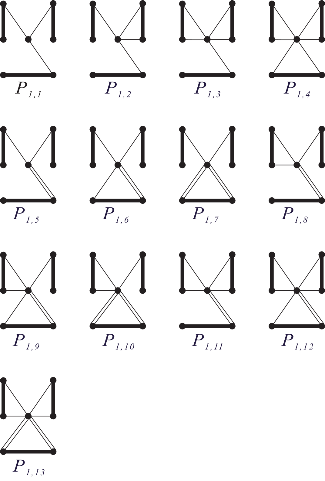
Figure 5. The $13$ finite-volume hyperbolic Coxeter $4$-polytopes with $7$ facets over polytope $P_{1}$.

7.3.2. Coxeter diagrams for $P_{2}$, $P_{3}$, $P_{5}$, and $P_{7}$ (Figure 6).

The hyperbolic Coxeter polytopes correspond to $P_{2,1}$ $P_{2.2}$, $P_{3.1}$, $P_{5,1}$, $P_{7,1}$, and $P_{7,2}$ have $3$, $3$, $3$, $2$, $1$, and $3$ ideal vertices and hyperbolic volume $\frac{1}{48}\pi^{2}$, $\frac{1}{54}\pi^{2}$, $\frac{1}{27}\pi^{2}$, $\frac{1}{48}\pi^{2}$, $\frac{5}{216}\pi^{2}$, and $\frac{31}{432}\pi^{2}$, respectively.

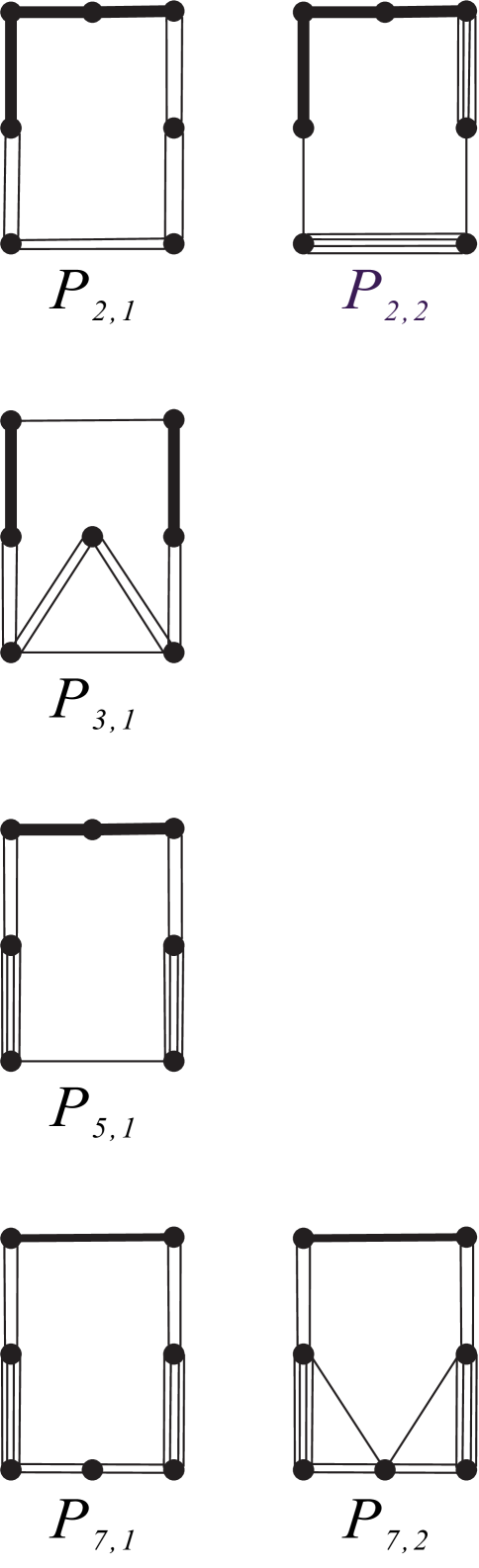
Figure 6. The 2, 1, 1, 2 finite-volume hyperbolic Coxeter $4$-polytopes with $7$ facets over polytopes $P_{2}$, $P_{3}$, $P_{5}$, and $P_{7}$, respectively.

7.3.3. Coxeter diagrams for $P_{6}$ (Figure 7–9).

There are $27$, $9$, and $1$ polytopes over $P_{6}$ with $2$, $3$, and $4$ ideal vertices, respectively. The minimum and maximum volumes are $\frac{1}{108}\pi^{2}$ and $\frac{5}{108}\pi^{2}$ of $P_{6,1}$ (with $2$ ideal vertex) and $P_{6,24}$ (with $2$ ideal vertices). Here the maximum is no obtained at the one with most ideal, i.e., $4$, vertices.

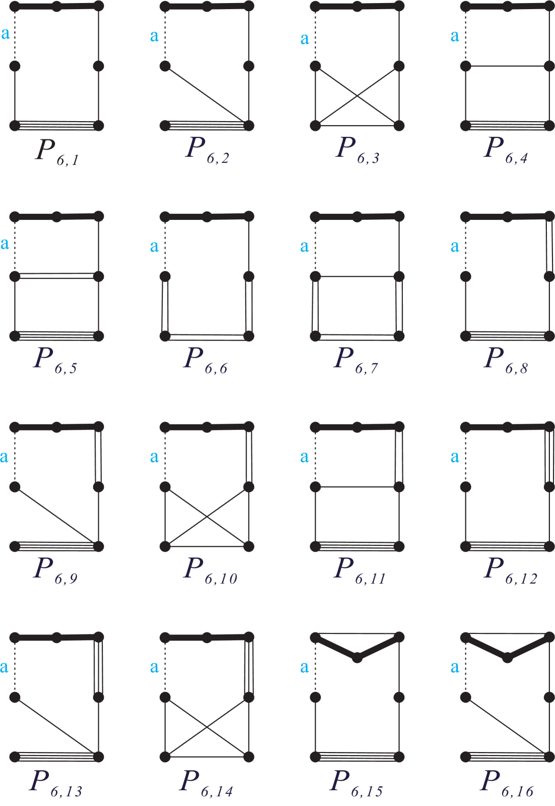
Figure 7. The $37$ finite-volume hyperbolic Coxeter $4$-polytopes with $7$ facets over polytope $P_{6}$ (part 1).

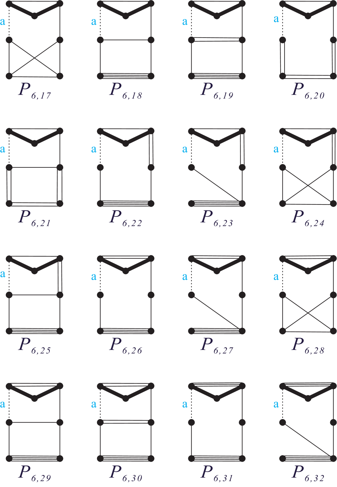
Figure 8. The $37$ finite-volume hyperbolic Coxeter $4$-polytopes with $7$ facets over polytope $P_{6}$ (part 2).

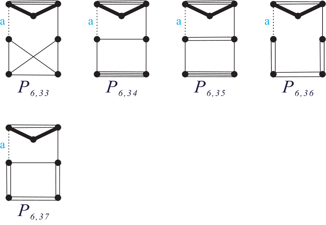
Figure 9. The $37$ finite-volume hyperbolic Coxeter $4$-polytopes with $7$ facets over polytope $P_{6}$ (part 3).

7.3.4. Coxeter diagrams for $P_{8}$ (Figure 10).

There are $7$, $2$, and $2$ polytopes over $P_{8}$ with $1$, $2$, and $3$ ideal vertices, respectively. The minimum and maximum volumes are $\frac{5}{288}\pi^{2}$ and $\frac{5}{54}\pi^{2}$ of $P_{8,1}$ (with $1$ ideal vertex) and $P_{8,8}$ / $P_{8,9}$ (with $1$ ideal vertex). Here the maxima is no obtained at the one with most ideal, i.e., $3$, vertices.

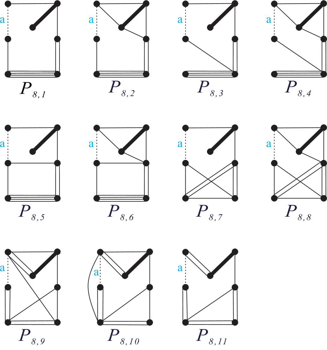
Figure 10. There are $11$ finite-volume hyperbolic Coxeter $4$-polytopes with $7$ facets over polytope $P_{8}$.

7.3.5. Coxeter diagrams for $P_{9}$ (Figure 11–19).

There are $58$, $33$, $23$, $6$, $6$, $2$, $4$, and $2$ polytopes over $P_{9}$ with $1$, $2$, $3$, $4$, $5$, $6$, $7$ and $10$ ideal vertices, respectively. The minimum and maximum volumes are achieved by $P_{9,46}$ (with $1$ ideal vertex), yielding $\frac{1}{1440}\pi^{2}$, and $P_{9,99}$ / $P_{9,100}$ (with $10$ ideal vertices), yielding $\frac{1}{9}\pi^{2}$. It is worth noting that certain hyperbolic Coxeter polytopes, such as $P_{19,7}$ etc., possess a facet with dihedral angles of $\frac{\pi}{2}$ and $\frac{\pi}{4}$ with other intersecting facets, allowing for the generation of numerous other polytopes through gluing.

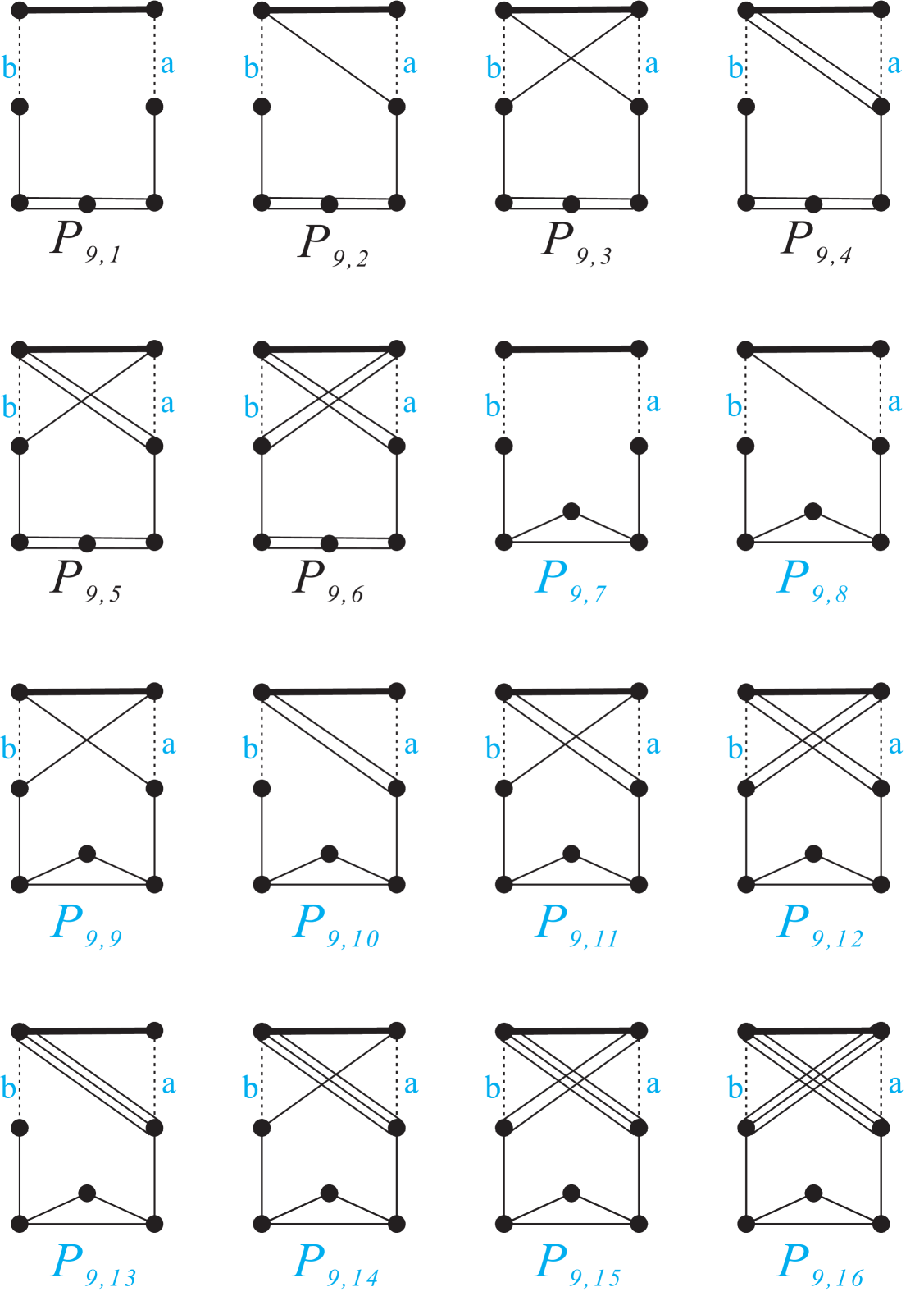
Figure 11. The $134$ finite-volume hyperbolic Coxeter $4$-polytopes with $7$ facets over polytope $P_{9}$ (part 1).

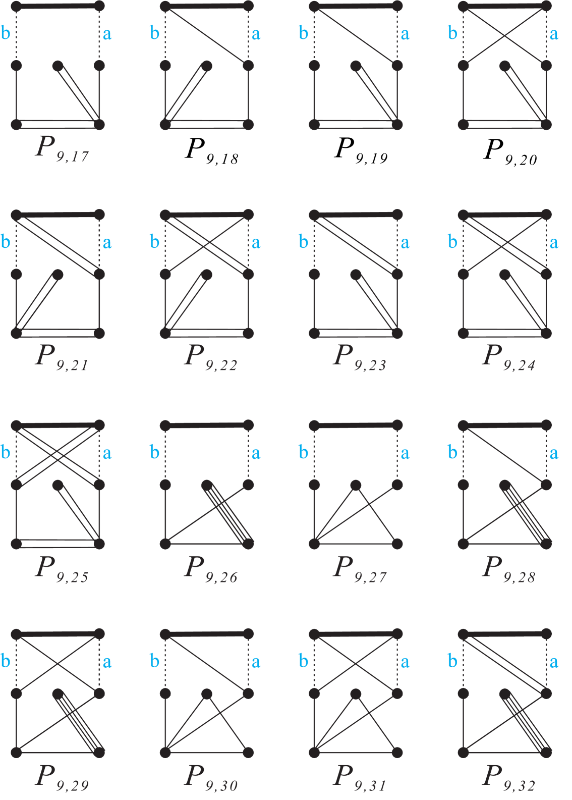
Figure 12. The $134$ finite-volume hyperbolic Coxeter $4$-polytopes with $7$ facets over polytope $P_{9}$ (part 2).

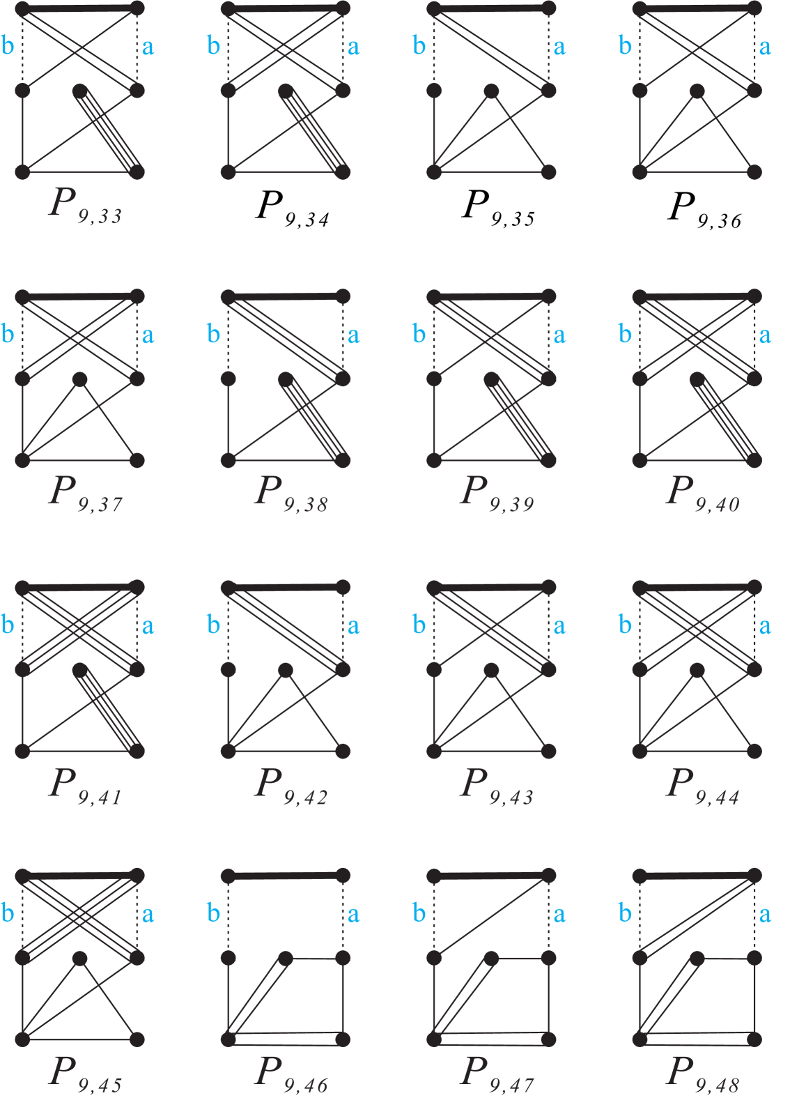
Figure 13. The $134$ finite-volume hyperbolic Coxeter $4$-polytopes with $7$ facets over polytope $P_{9}$ (part 3).

Figure 14. The $134$ finite-volume hyperbolic Coxeter $4$-polytopes with $7$ facets over polytope $P_{9}$ (part 4).

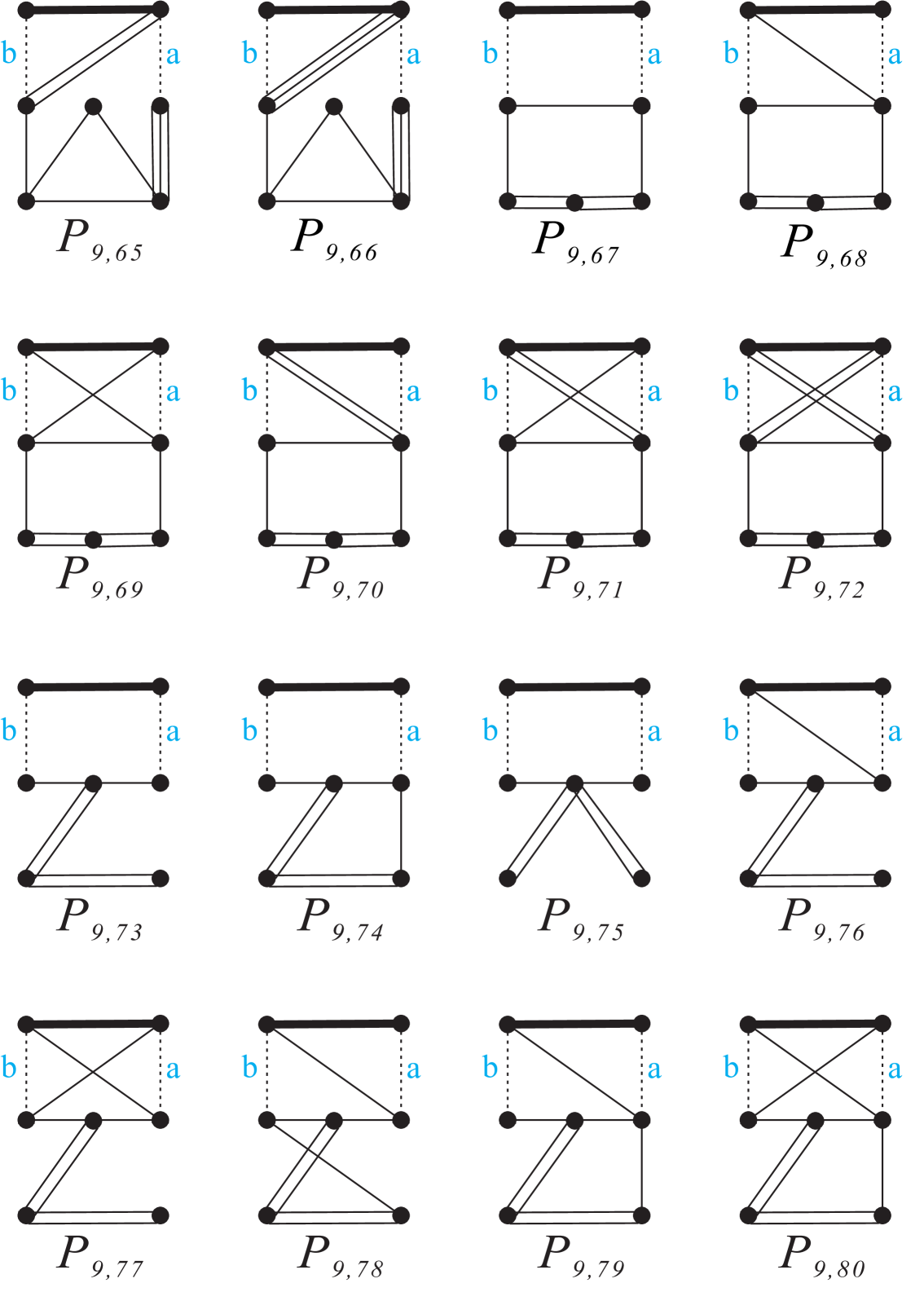
Figure 15. The $134$ finite-volume hyperbolic Coxeter $4$-polytopes with $7$ facets over polytope $P_{9}$ (part 5).

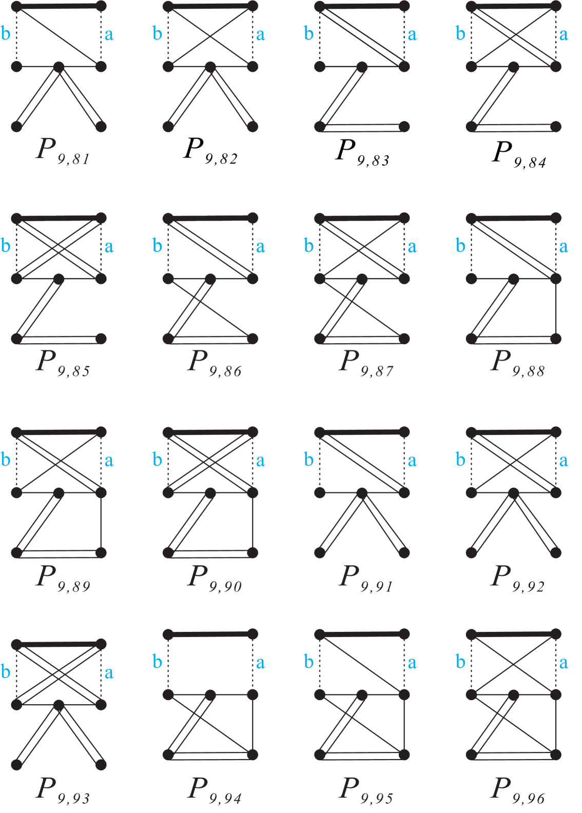
Figure 16. The $134$ finite-volume hyperbolic Coxeter $4$-polytopes with $7$ facets over polytope $P_{9}$ (part 6).

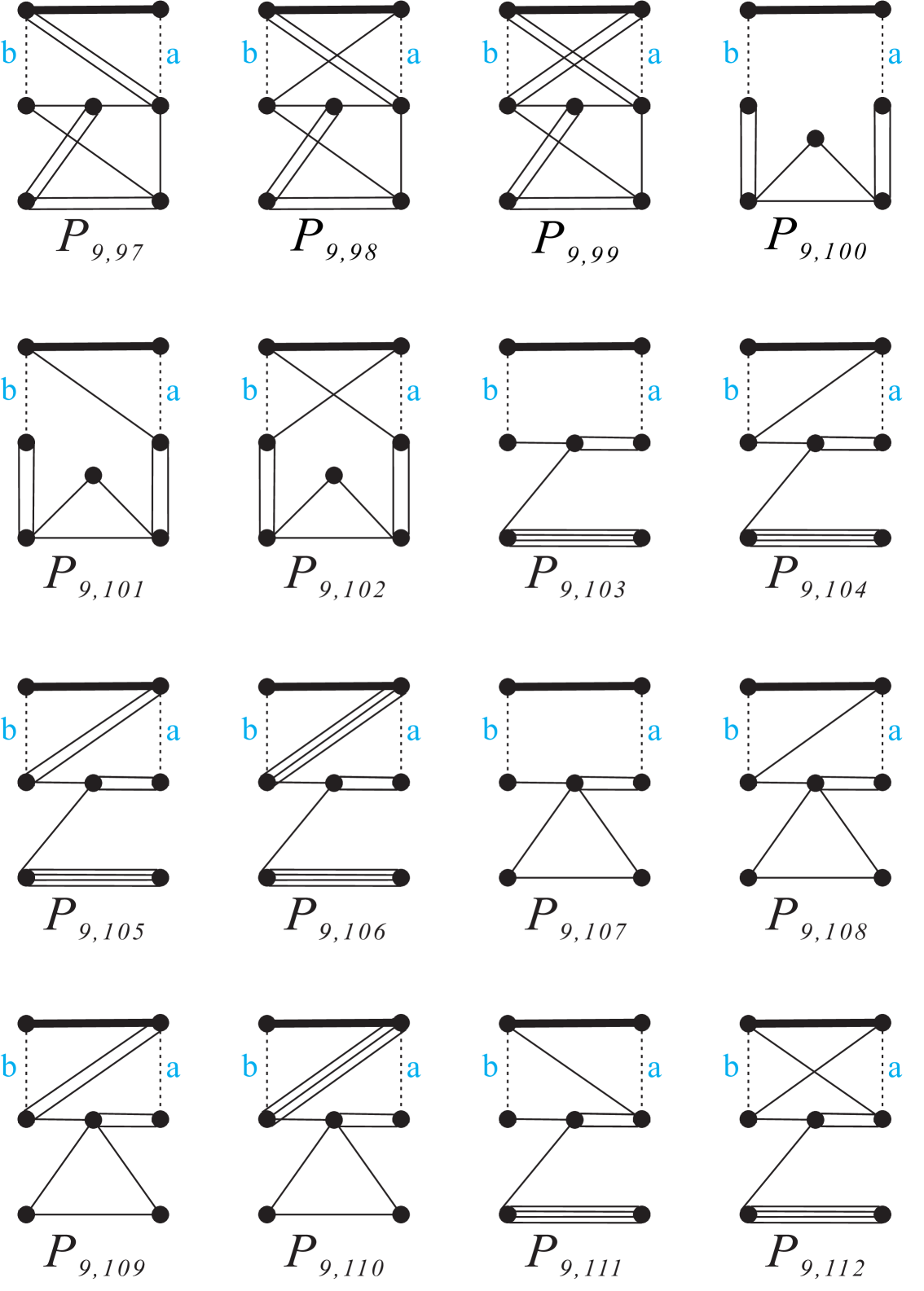
Figure 17. The $134$ finite-volume hyperbolic Coxeter $4$-polytopes with $7$ facets over polytope $P_{9}$ (part 7).

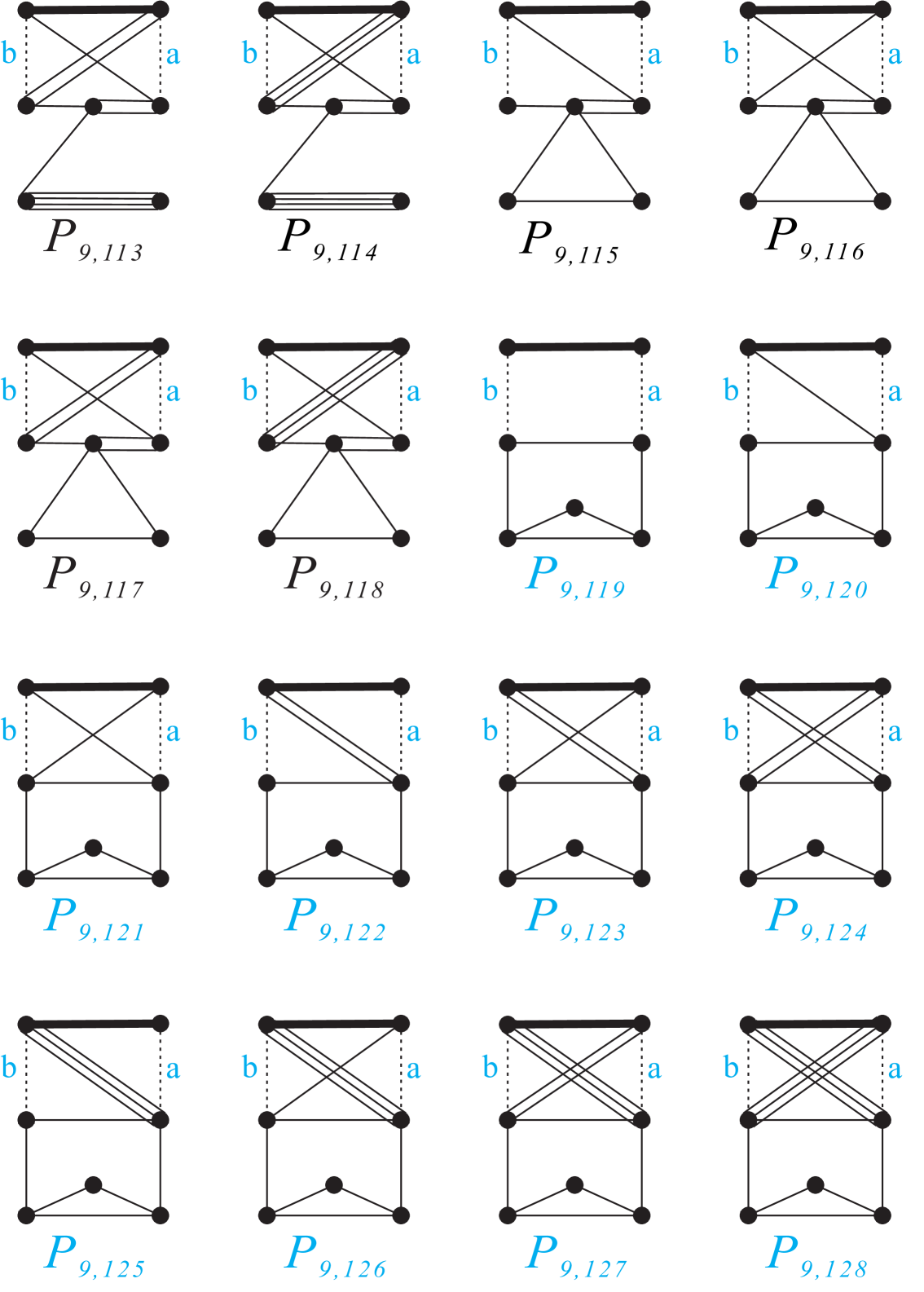
Figure 18. The $134$ finite-volume hyperbolic Coxeter $4$-polytopes with $7$ facets over polytope $P_{9}$ (part 8).

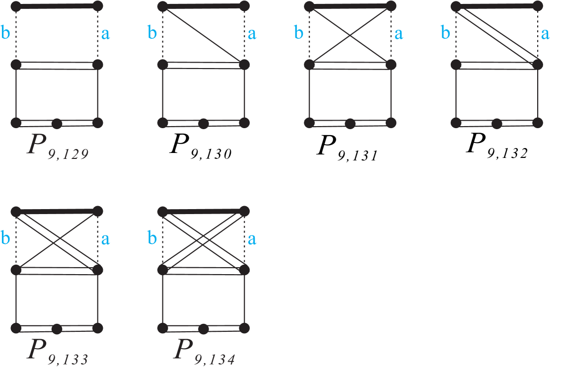
Figure 19. The $134$ finite-volume hyperbolic Coxeter $4$-polytopes with $7$ facets over polytope $P_{9}$ (part 9).

7.3.6. Coxeter diagrams for $P_{10}$ (Figure 20).

The hyperbolic Coxeter polytopes correspond to $P_{10,1}$–$P_{10,4}$ have $2$, $2$, $3$, and $3$ ideal vertices and hyperbolic volume $\frac{5}{216}\pi^{2}$ (minimum), $\frac{25}{864}\pi^{2}$, $\frac{5}{108}\pi^{2}$, and $\frac{25}{432}\pi^{2}$ (maximum), respectively.

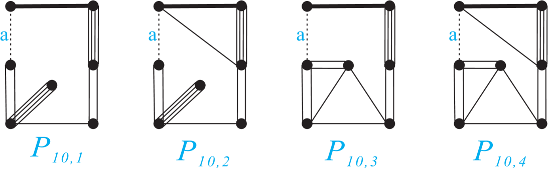
Figure 20. The $4$ finite-volume hyperbolic Coxeter $4$-polytopes with $7$ facets over polytope $P_{10}$.

7.3.7. Coxeter diagrams for $P_{11}$ (Figure 21).

There are $8$, $4$, and $1$ polytopes over $P_{11}$ with $8$, $4$, and $1$ ideal vertex, respectively. The minimum and maximum volumes are $\frac{143}{5400}\pi^{2}$ and $\frac{1}{90}\pi^{2}$ of $P_{11,11}$ (with $1$ ideal vertex) and $P_{11,2}$ (with $1$ ideal vertex), respectively. Here the maximum is no obtained at the one with most ideal, i.e., $3$, vertices.

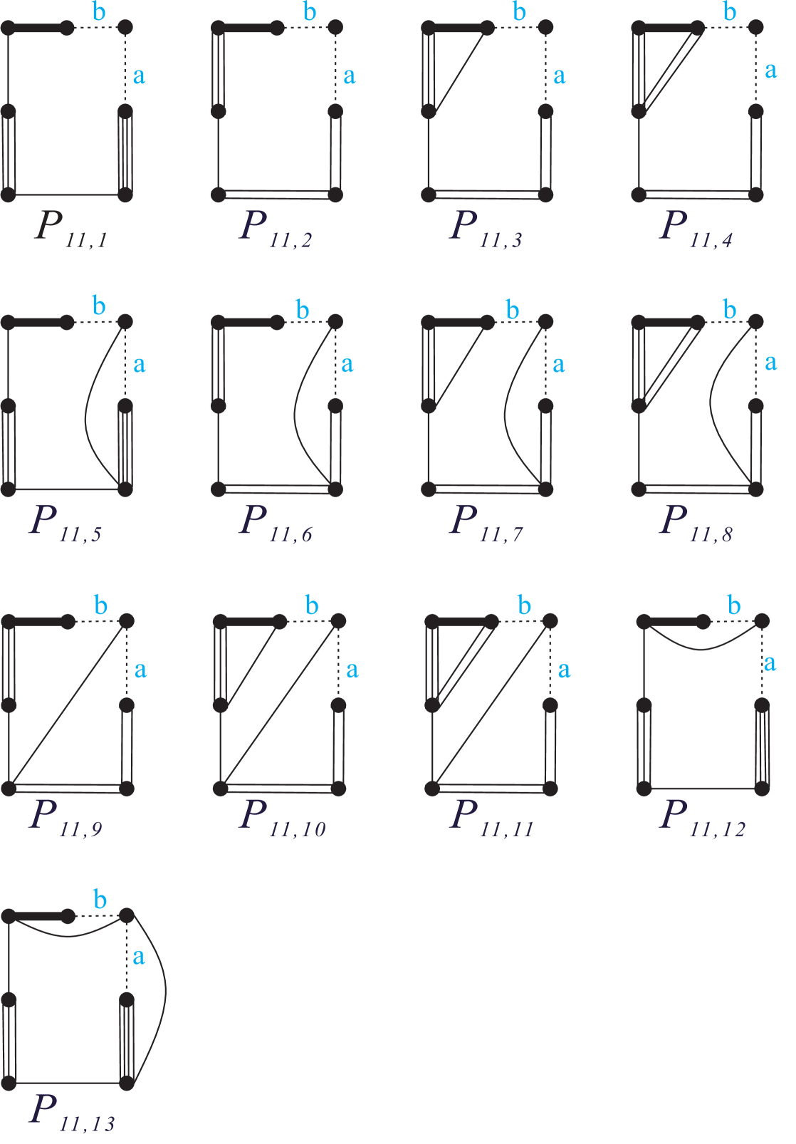
Figure 21. The $13$ finite-volume hyperbolic Coxeter $4$-polytopes with $7$ facets over polytope $P_{11}$.

7.3.8. Coxeter diagrams for $P_{13}$ (Figure 22).

There are $3$, $1$, $2$, and $2$ polytopes over $P_{13}$ with $0$ (compact), $1$, $2$, and $4$ ideal vertices, respectively. The minimum and maximum volumes are achieved by $P_{13,7}$ (with $1$ ideal vertex), yielding $\frac{113}{4320}\pi^{2}$, and $P_{13,5}$ / $P_{13,6}$ (both with $4$ ideal vertices), yielding $\frac{1}{9}\pi^{2}$. The volumes of any compact polytopes with this combinatorial type lie within this range.

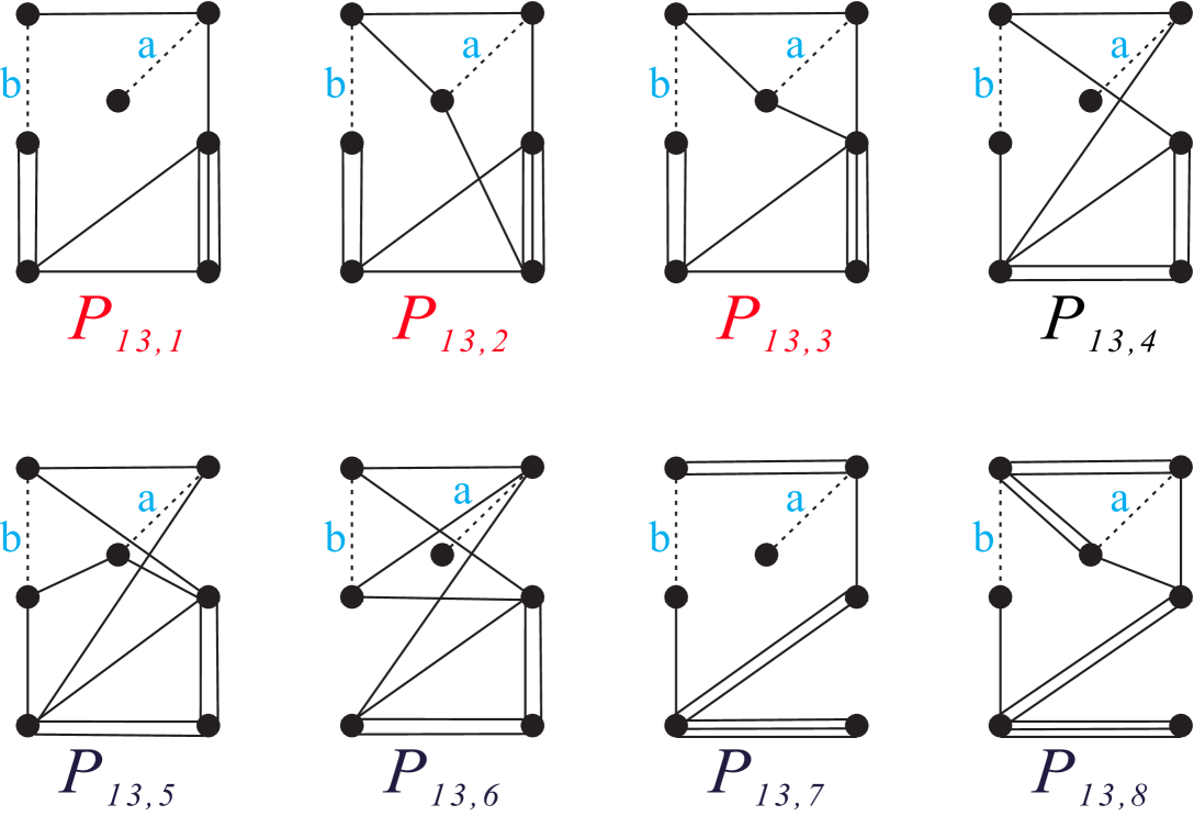
Figure 22. The $8$ finite-volume hyperbolic Coxeter $4$-polytopes with $7$ facets over polytope $P_{13}$.

7.3.9. Coxeter diagrams for $P_{14}$ (Figure 23).

There are only compact hyperbolic Coxeter polytopes over the combinatorial type $P_{14}$. The minimum and maximum volumes are $\frac{13}{900}\pi^{2}$ and $\frac{11}{144}\pi^{2}$ of $P_{14,1}$ and $P_{14,7}$, respectively.

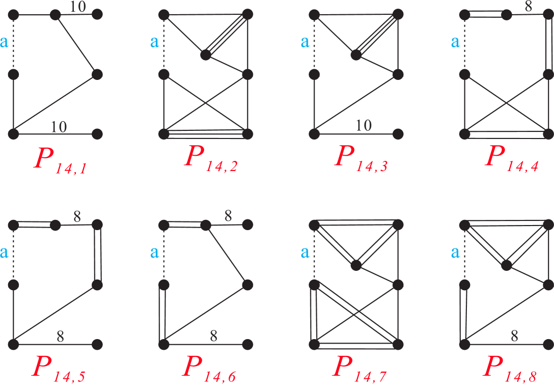
Figure 23. The $8$ finite-volume hyperbolic Coxeter $4$-polytopes with $7$ facets over polytope $P_{14}$.

7.3.10. Coxeter diagrams for $P_{16}$ (Figure 24–29).

There are $29$, $21$, $9$, $6$, $9$, $4$, and $3$ polytopes over $P_{16}$ with $0$ (compact), $1$, $2$, $3$, $4$, $5$, and $6$ ideal vertices, respectively. The minimum and maximum volumes are achieved by $P_{19,34}$ (with $1$ ideal vertex), yielding $\frac{1}{1440}\pi^{2}$, and $P_{19,70}$ / $P_{19,77}$ / $P_{19,81}$ (with $6$ ideal vertices), yielding $\frac{5}{72}\pi^{2}$. The volumes of any compact polytopes with this combinatorial type lie within this range.

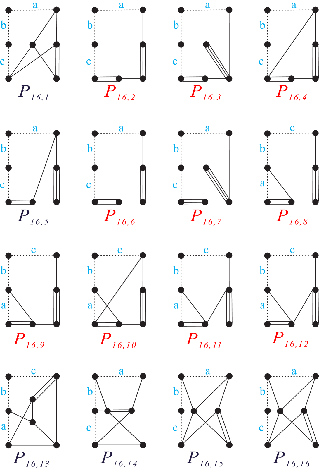
Figure 24. The $81$ finite-volume hyperbolic Coxeter $4$-polytopes with $7$ facets over polytope $P_{16}$ (part 1).

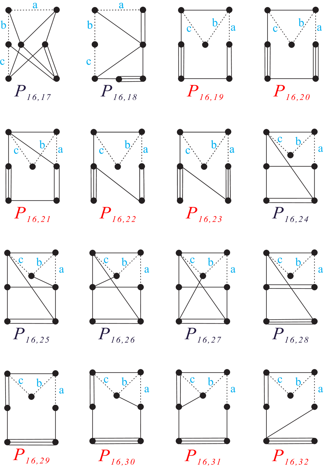
Figure 25. The $81$ finite-volume hyperbolic Coxeter $4$-polytopes with $7$ facets over polytope $P_{16}$ (part 2).

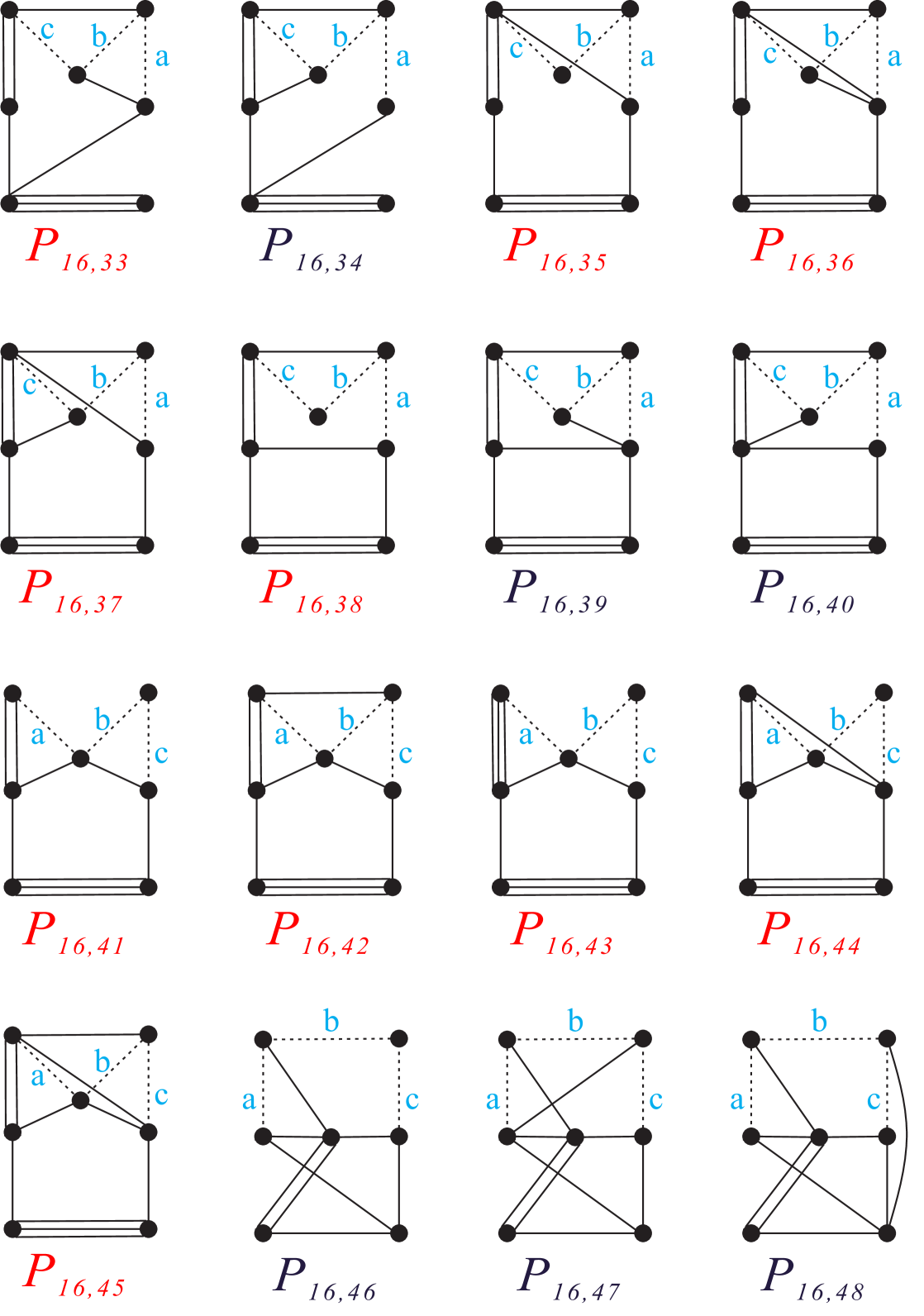
Figure 26. The $81$ finite-volume hyperbolic Coxeter $4$-polytopes with $7$ facets over polytope $P_{16}$ (part 3).

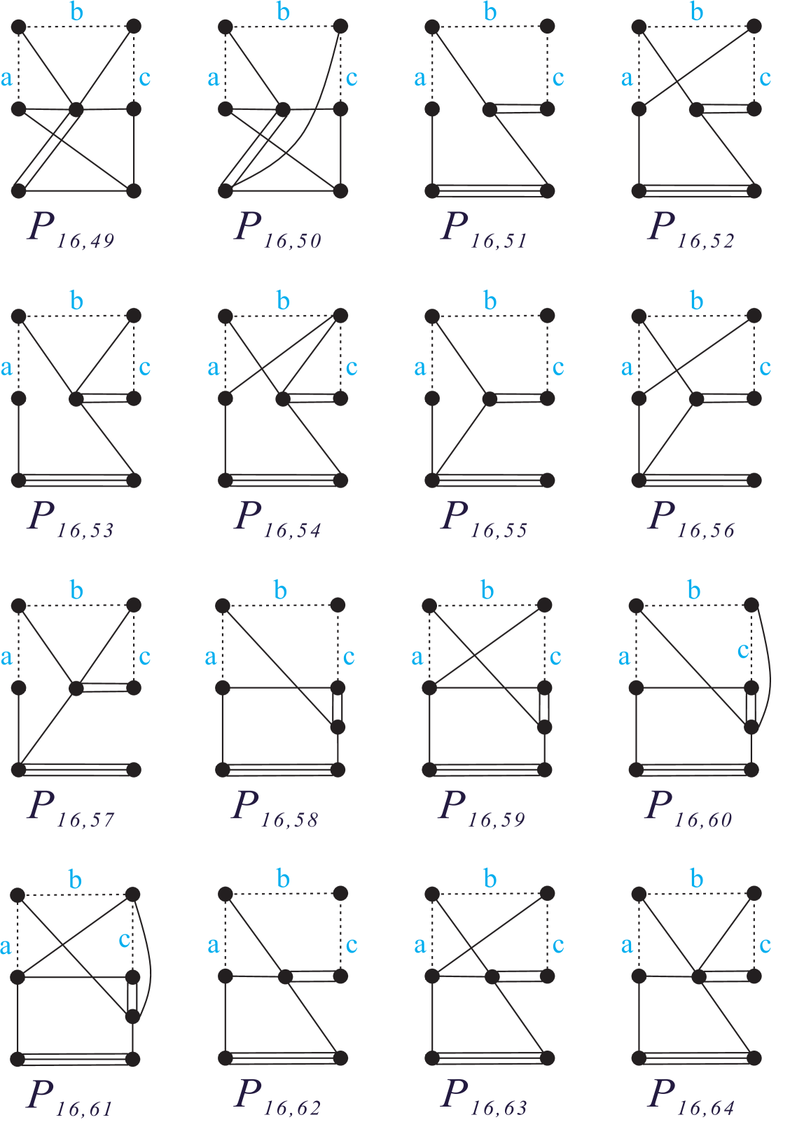
Figure 27. The $81$ finite-volume hyperbolic Coxeter $4$-polytopes with $7$ facets over polytope $P_{16}$ (part 4).

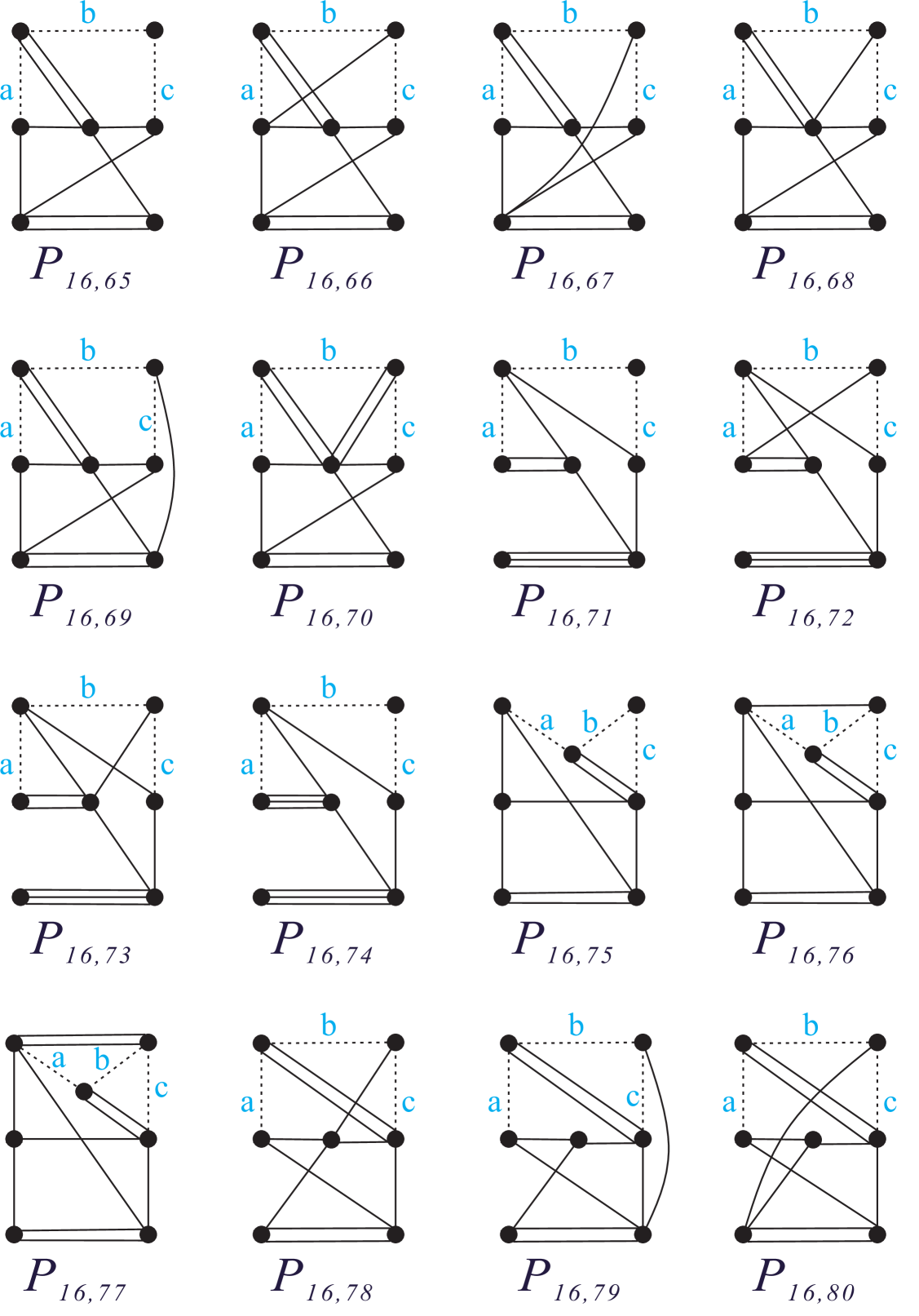
Figure 28. The $81$ finite-volume hyperbolic Coxeter $4$-polytopes with $7$ facets over polytope $P_{16}$ (part 5).

Figure 29. The $81$ finite-volume hyperbolic Coxeter $4$-polytopes with $7$ facets over polytope $P_{16}$ (part 6).

References

- [All06] D. Allcock. Infinitely many hyperbolic Coxeter groups through dimension 19. Geom. Topol. 10 (2006), 737–758.
- [Ale23] S. Alexandrov. Lannér diagrams and combinatorial properties of compact hyperbolic Coxeter polytopes. Trans. Amer. Math. Soc. 376 (2023), no. 10, 6989–7012.
- [And] E. M. Andreev. Convex polyhedra in Lobachevskii spaces (Russian). Math. USSR Sbornik 10 (1970), 413–440.
- [And] E. M. Andreev. Convex polyhedra of finite volume in Lobachevskii space (Russian). Math. USSR Sbornik 12 (1970), 255–259.
- [BD98] B. Bagchi and B. Datta. A structure theorem for pseudomanifolds. Discrete Math, 188 (1998), no.1, 40–60.
- [BDR23] N. Bogachev, S. Douba and J. Raimbault. Infinitely many commensurability classes of compact Coxeter polyhedra in and . . arXiv:2309.07691.
- [Bor98] R. Borcherds. Coxeter groups, Lorentzian lattices, and K3 surfaces. Internat. Math. Res. Notices (1998), no. 19, 1011–1031.
- [Bou68] N. Bourbaki. Éléments de mathématique. Fasc. XXXIV. Groupes et algèbres de Lie. Chapitre IV: Groupes de Coxeter et systèmes de Tits. Chapitre V: Groupes engendrés par des réflexions. Chapitre VI: systèmes de racines.(French), Hermann, Paris, 1968.
- [Bug84] V. O. Bugaenko. Groups of automorphisms of unimodular hyperbolic quadratic forms over the ring Vestnik Moskov. Univ. Ser. I Mat. Mekh. (1984), no. 5, 6–12.
- [Bug92] V. O. Bugaenko. Arithmetic crystallographic groups generated by reflections, and reflective hyperbolic lattices. Lie groups, their discrete subgroups, and invariant theory, Adv. Sov. Math. 8 (1992), 33–55.
- [Cox34] H. S. M. Coxeter. Discrete groups generated by reflections. Ann. of Math. (2) 35 (1934), no. 3, 588–621.
- [Ess94] F. Esselmann. Über kompakte hyperbolische Coxeter-Polytope mit wenigen Facetten. Universit at Bielefeld, SFB343, (1994) preprint 94-087.
- [Ess96] F. Esselmann. The classification of compact hyperbolic Coxeter -polytopes with facets. Comment. Math. Helv. 71 (1996), no. 2, 229–242.
- [F] A. Felikson http://www.maths.dur.ac.uk/users/anna.felikson/Polytopes/polytopes.html
- [FT] A. Felikson, P. Tumarkin. On hyperbolic Coxeter polytopes with mutually intersecting facets. J. Combin. Theory Ser. A 115 (2008), no. 1, 121–146.
- [Gan59] F. R. Gantmacher. The theory of matrix. Chelsca Publishing Company, 1959.
- [Grü67] B. Grünbaum. Convex Polytopes. Springer, 2003.
- [Gug17] Hyperbolic isometries in (in-)finite dimensions and discrete reflection groups: theory and computations. Ph.D. thesis no. 2008, Université de Fribourg 2017.
- [ImH90] H.-C. Im Hof. Napier cycles and hyperbolic Coxeter groups, Bull. Soc. Math. Belg. Sér. A 42 (1990), no. 3, 523–545.
- [Jac17] M. Jacquemet On hyperbolic Coxeter n-cubes. European J. Combin. 59 (2017), 192–203.
- [JT18] M. Jacquemet and S. Tschantz. All hyperbolic Coxeter n-cubes. J. Combin. Theory Ser. A 158 (2018), 387–406.
- [Kap74] I. M. Kaplinskaya. The discrete groups that are generated by reflections in the faces of simplicial prisms in Lobačevskiĭ spaces.(Russian). Mat. Zametki 15 (1974), 159–164.
- [Kel14] R. Kellerhals. Hyperbolic orbifolds of minimal volume. Comput. Methods Funct. Theory 14 (2014), 465–481.
- [KP11] R. Kellerhals and G. Perren. On the growth of cocompact hyperbolic Coxeter groups. Eur. J. Comb., 32, no.8, (2011), 1299–1316.
- [KM13] A. Kolpakov and B. Martelli. Hyperbolic four-manifolds with one cusp. Geom. Funct. Anal. 23(2013), no. 6, 1903–1933.
- [Kos67] J. L. Koszul. Lectures on hyperbolic Coxeter group. University of Notre Dame, 1967.
- [Lan50] F. Lannér. On complexes with transitive groups of automorphisms. Comm. Séem. Math. Univ. Lund, 11 (1950), 71 pp.
- [Mak65] V. S. Makarov. On one class of partitions of Lobačevskiĭ space. Dokl. Akad. Nauk SSSR 161 (1965), 277–278.
- [Mak66] V. S. Makarov. On one class of discrete groups of Lobachevskian space having an infinite fundamental region of finite measure. Dokl. Akad. Nauk SSSR 167 (1966), 30–33.
- [Mak68] V. S. Makarov. On Fedorov groups of four- and five-dimensional Lobachevsky spaces. Issled. po obshch. algebre. no. 1, Kishinev St. Univ., 1970, 120–129 (Russian).
- [MZ21] J. Ma and F. Zheng. Hyperbolic 4-manifolds over the 120-cell. Math. Comp. 90 (2021), 2463-2501.
- [MZ22] J. Ma and F. Zheng. Compact hyperbolic Coxeter four-dimensional polytopes with eight facets. https://arxiv.org/abs/2201.00154 To appear in J. Algebra. Comb.
- [MZ23] J. Ma and F. Zheng. Compact hyperbolic Coxeter five-dimensional polytopes with nine facets. Transform. Groups (2023). https://doi.org/10.1007/s00031-023-09830-3
- [P1882] H. Poincaré. Theorié des groupes fuchsiens (French). Acta Math. 1 (1882), no. 1, 1–76.
- [Pro87] M. N. Prokhorov. The absence of discrete reflection groups with non-compact fundamental polyhedron of finite volume in Lobačevskiĭ space of large dimension. Math. USSR Izv. 28 (1987), 401–411.
- [Rob15] M. Roberts. A Classification of Non-Compact Coxeter Polytopes with Facets and One Non-Simple Vertex arXiv:1511.08451.
- [Rus89] O. P. Rusmanov. Examples of non-arithmetic crystallographic Coxeter groups in -dimensional Lobačevskiĭ space for . Problems in Group Theory and Homology Algebra, Yaroslavl, 1989, 138–142 (Russian).
- [Tum03] P. Tumarkin. Non-compact hyperbolic Coxeter n-polytopes with n+3 facets, short version (3 pages). Russian Math. Surveys 58 (2003), 805-806.
- [Tum] P. Tumarkin. Hyperbolic Coxeter -polytopes with facets. Math. Notes 75 (2004), 848–854.
- [Tum] P. Tumarkin. Hyperbolic Coxeter -polytopes with facets. Trans. Moscow Math. Soc. (2004), 235–250.
- [Tum07] P. Tumarkin. Compact hyperbolic Coxeter n-polytopes with facets. Electron. J. Combin., 14 (2007), no. 1, Research Paper 69, 36 pp.
- [Vin67] E. B. Vinberg. Discrete groups generated by reflections in Lobačevskiĭ spaces. Mat. USSR Sb. 1 (1967), 429–444.
- [Vin69] E. B. Vinberg. Some examples of crystallographic groups in Lobačevskiĭ spaces. Math. USSR-Sb. 7 (1969), no. 4, 617–622.
- [Vin72] E. B. Vinberg. On groups of unit elements of certain quadratic forms. Math. USSR Sb. 16 (1972), 17–35.
- [Vin] E. B. Vinberg. The absence of crystallographic groups of reflections in Lobačevskiĭ spaces of large dimension. Trans. Moscow Math. Soc. 47 (1985), 75–112.
- [Vin] E. B. Vinberg. Hyperbolic reflection groups. Russian Math. Surveys 40 (1985), 31–75.
- [Vin93] E. B. Vinberg, editor. Geometry II - Spaces of Constant Curvature. Springer, 1993.
- [Vin15] E. B. Vinberg. Nonarithmetic hyperbolic reflection groups in higher dimension. Moscow Math J. 15 (2015), no. 3, 593–602.
- [VK78] E. B. Vinberg and I. M. Kaplinskaya. On the groups and . Soviet Math. Dokl. 19 (1978), 194–197.