Sacred Ecology: The Environmental Impact of African Traditional Religions

Abstract

Do religions codify ecological principles? This paper explores theoretically and empirically the role religious beliefs play in shaping environmental interactions. We study African Traditional Religions (ATR) which place forests within a sacred sphere. We build a model of non-market interactions of the mean-field type where the actions of agents with heterogeneous religious beliefs continuously affect the spatial density of forest cover. The equilibrium extraction policy shows how individual beliefs and their distribution among the population can be a key driver of forest conservation. The model also characterizes the role of resource scarcity in both individual and population extraction decisions. We test the model predictions empirically relying on the unique case of Benin, where ATR adherence is freely reported. Using an instrumental variable strategy that exploits the variation in proximity to the Benin-Nigerian border, we find that a 1 standard deviation increase in ATR adherence has a 0.4 standard deviation positive impact on forest cover change. We study the impact of historically belonging to the ancient Kingdom of Dahomey, birthplace of the Vodun religion. Using the original boundaries as a spatial discontinuity, we find positive evidence of Dahomey affiliation on contemporary forest change. Lastly, we compare observed forest cover to counterfactual outcomes by simulating the absence of ATR beliefs across the population.

JEL Codes: Z12, Q5, C7
Keywords: African Traditional Religions, Beliefs, Forests, Non-market interactions.

Preliminary Draft - Please do not circulate without authors’ permission.

1 Introduction

Open your eyes, stranger, and know where to step. Here, a tree is not a tree, a spring is not a spring. Everything is mysterious and mystical.

– Eustache Prudencio, Vents du Lac

Religion is a powerful way by means of which societies organize their worldviews and shape human behaviour. Research shows that religious beliefs play an important role in determining economic outcomes and attitudes (Guiso et al., 2006; Iannaccone and Bainbridge, 2009; Iyer, 2016). Studies have highlighted the importance of cultural factors in the use of common pool resources (Hayo and Vollan, 2012; Handberg and Angelsen, 2015), formation of environmental preferences (Videras et al., 2012; Filippini and Wekhof, 2021) and provision of public goods such as forests (Alesina et al., 2019; Barba and Jaimovich, 2022). Although these studies identify certain aspects of culture relevant for environmental outcomes, the analysis of the religious dimension of human ecology remains scant in the economic literature.

The influence religion can have on an individual’s worldview of prosocial behaviour and interpersonal relationships is well established. What is less explored, however, is how religion can shape human interactions with the environment. The anthropologist Reichel-Dolmatoff (1976), for example, suggested that aboriginal cosmologies and myth structures, together with the ritual behavior derived from them, represent in all respects a set of ecological principles and that these formulate a system of social and economic rules. The primary thesis underlying the link between religion and the environment is that an individual’s interaction with the ecosystem is often conditioned by cultural beliefs, rituals and values that are codified within the principles of the religion. It is therefore of relevance to ask whether adherence to beliefs that facilitate such an unique worldview of nature can significantly impact environmental outcomes. The objective of this paper is to examine this premise by focusing on African Traditional Religions (ATR) in whose cosmology the forest is a fundamental sacred symbol. In doing so, we investigate if religion, and in particular adherence to ATR, exerts an independent effect on forest cover dynamics. Combining applied theory with empirical evidence, we show that ATR adherence indeed has a causal and positive impact on forest cover change.

In order to formalize the role of beliefs in shaping the interplay between individuals and the environment we build a model with non-market interactions of the mean field type. We consider an individual who draws utility from the extraction of forest resources calibrated by her level of adherence to ATR and where the evolution of the resource for the continuum of agents is described by a diffusion process. The framework introduces two important features: heterogeneity in belief levels and a quantity representing the cost associated with resource scarcity which is dependent on the distribution of the overall forest cover. The mechanism that shapes interactions between agents is such that an individual can incorporate into her preferences and decisions the information on the distribution of forest cover within the population at the anticipated equilibrium. As each individual has her own level of exogenous adherence to ATR, the density of the forest resource will depend on the density of such ATR beliefs.

Solving analytically for the equilibrium strategy, we highlight two crucial model predictions. First, we find that for any given population distribution of ATR beliefs, a higher individual adherence implies a reduced forest extraction. Secondly, addressing the spillover effects, the model predicts that changes in the belief distribution ranked in terms of first-order stochastic dominance can independently affect both individual and population consumption decisions via resource scarcity. Specifically, we find that an increase in the average ATR adherence within the population implies an increase in individual forest extraction, therefore, emphasising the counter-intuitive interplay between global and individual (or any localized) levels of ATR adherence.

We empirically test the model predictions by leveraging the rich and unique historical experience of Benin which helps overcome issues of identification of religion effects. These are primarily concerned with self selection and the widespread under-reporting of ATR in Sub Saharan Africa which can be traced back to the colonial and missionary efforts to civilize individuals and promote Christianity as the socially acceptable choice. Within Benin, adherence of ATR is often inherited and steeped in history and tradition due to the hegemonic role played by the ancient Kingdom of Dahomey. The Kingdom was not only the birthplace of Vodun, Benin’s largest traditional religion, but it also famously and fiercely resisted evangelization until the French colonisation. Subsequently, in 1992 in a move to reconcile with its past and culture, Vodun was rehabilitated, given its own national holiday and today enjoys the same privilege and status as Christianity and Islam. Finally, within the context of an environmental profile, while deforestation rates in Benin continue to be high at 2.2% per annum, nevertheless, at a local level the forests continue to serve a crucial social role as a place for cultural and religious activities. The country is estimated to have about 3000 sacred forests and groves, often utilized for traditional rituals.

To investigate the impact of ATR adherence on forest cover change, we use four waves of nationally representative geo-localized Demographic and Health Surveys (DHS) from 1996 to 2016 and match these to a grid with cell resolution of 10 kms $\times$ 10 kms. This allows to circumvent the cross-sectional nature of DHS and create an unbalanced panel. Using the information on religion, we construct a measure of ATR adherence as the share of individuals who self report their religion as ATR in each grid cell. For the key outcome of interest, 5 year average annual change in forest cover, we take advantage of a high resolution environmental data by NASA which provides annual global fractional vegetation cover for the time period 1982 - 2016. In the econometric specifications we exploit the within cell panel variation by controlling for cell fixed effects and unobserved common time shocks and document a robust positive relationship between ATR adherence and five year average annual change in forest cover. Exploring the externality arising from global adherence on localized forest dynamics, we introduce as an additional explanatory variable the ATR adherence averaged over states (administrative division one). Consistent with the model predictions of two contrasting effects, we find that while cell level ATR continues to have a positive effect, an increase in state ATR adherence is associated with a negative impact on forest change within the grid cell.

Addressing the endogeneity concerns, we use an instrumental variable (IV) approach by drawing upon the close historical and contemporary relationship between Nigeria and Benin. Based on the significant impact the former had on the Béninois religious landscape, the proposed instrument for ATR adherence is the distance from the Nigerian border interacted with a linear time trend capturing the generalized decrease in ATR across the country. Specifically, Benin has been influenced by two prominent nineteenth century religious movements originating in Nigeria leading to the persistent displacement of traditional religions and the diffusion of Christianity and Islam. The key identification assumption is that, conditional on the included controls, the instrument affects only the spatial distribution of ATR and is not correlated with any unobserved local factors that might influence forest cover dynamics. The IV estimates are sizeable and positive, showing that a 1 standard deviation increase in ATR adherence has a 0.43 standard deviation positive impact on the five year average annual change in forest cover. We complement these findings with further evidence by exploiting the nineteenth century boundaries of the Kingdom of Dahomey within a spatial regression discontinuity design. Vodun was Dahomey’s state religion and was closely linked to the legitimacy of the monarchy. We estimate the impact of historically belonging to the Kingdom on contemporary forest cover change over three timescales: 5, 10 and 15 years average annual change. We find that grid cells within Dahomey have a higher likelihood of having a positive impact on both 10 and 15 years average annual change in forest cover.

The model predicts that the level of individual beliefs directly influences resource extraction, indicating that believing is a mechanism through which religion matters for environmental outcomes (McCleary and Barro, 2006). Furthermore, it assumes forest extraction and ATR beliefs to be substitutes, implying that an increase in adherence reduces the marginal utility derived from destruction of forest resources. The way for the belief-resource substitutability to manifest is via a set of attitudes and values within adherents that reflect a spirit of sustainability. This view is consistent with the Weberian framework which considers religiosity as an independent variable that influences outcomes by fostering individual traits and values (Weber, 1904). In the case of Benin, where the agricultural sector employs more than 50 percent of the population and is dominated by subsistence farming, this spirit would primarily be reflected in a sustainable interaction with land. We find suggestive evidence that households with ATR heads are more likely to adopt sustainable agricultural practices. We find that ATR adherence has no significant correlation with land degradation and grid cells falling within the upper quartile of ATR adherence distribution have a 22% lower probability of deforesting for agricultural purposes.

In the last section, we estimate the model parameters and show that the spatial distribution of forest and beliefs implied by the estimated model fits well the joint empirical density of ATR and forest cover. We then build a counterfactual spatial forest cover distribution where we remove all heterogeneity in beliefs among the population and impose for all grid cells the ATR adherence to be zero. For this scenario we find the forest cover across Benin is substantially reduced, with an average forest loss of approximately 7%.

The paper makes several contributions to the literature. First, it contributes to the theoretical literature on non-market interactions which typically postulate individual’s interdependence and analyzes the macro behavior that emerges (Glaeser and Scheinkman, 2000; Brock and Durlauf, 2001; Guéant et al., 2011; Acemoglu and Jensen, 2015). Building on these, the model introduces two novel features. First, the model successfully couples beliefs and ecological dynamics by means of strategic decision making by a continuum of interacting agents in a continuous time framework. Second, it establishes a framework for analysing the effect of belief heterogeneity in mean-field interactions which remains tractable whilst maintaining the essence of the complexity of the problem. Essentially, by providing such a general setup the model allows one to explore any cultural and social dimension influencing resource use decisions.

The second primary contribution of the paper is to the larger work on economics of religion (Iannaccone, 1998; Guiso et al., 2003; McCleary and Barro, 2006; Iyer, 2016; Carvalho et al., 2019). This research focuses on the environment, which the literature on religion has not yet systematically studied within a quantitative or theoretical framework. The only contribution in this area is by Owen and Videras (2007) who empirically study the impact of culture, as expressed by religious beliefs, on generating public goods contributions. Our work complements their results and takes a substantial step further in discovering causal relations, mechanisms and theoretical underpinnings. In addition, by focusing on ATR, the paper refines our understanding of the impact of religions beyond the Abrahamic faiths and within the developing world context (Iyer, 2016). The results of this paper indicate that the lessons of traditional knowledge codified in religious beliefs, especially of the ecological kind, can have practical significance for the rest of the world. This works also adds to the burgeoning research on ATR such as Stoop et al. (2019) who estimate a negative impact of ATR adherence on the uptake of medical and preventive health care; Alonso et al. (2016) study the role of Vodun in the management of fisheries and Alidou (2021) shows the effect of ATR beliefs on parental investment.

The paper proceeds as follows. Section 2 provides background on ATR. Section 3 presents the model. Section 4 provides historical and contemporary overview of Benin and introduces the data and descriptive evidence. Section 5 presents the instrumental variable and spatial RDD strategies. Section 6 presents the structural estimates and model predictions. Section 7 concludes.

2 African Traditional Religions & Forests

ATR refers to the indigenous religions of the African continent and encapsulate the significant belief system that depict African beliefs, thought patterns, and ritual practices (Parrinder, 1949; Idowu, 1973; Mbiti, 1990; Opoku, 1993). It presents an integrated cosmogony between the gods and nature, and thus the adherents view themselves as symbiotically related to the natural environment as it is closely correlated to the spiritual world. The worldview is one where the spiritual beings are all around, present in the natural surroundings of which people are a part. This translates to a belief that to respect the spiritual is to respect the environment, and the destruction of the land is traditionally seen as a violation of the spirit world (Aderibigbe and Falola, 2022). This is especially true for West Africa where nature’s sacred element has led to large pantheons of spirits and divinities. Many ATR contain myths about the creation of the world, why it looks and functions the way it does; and frequently nature provides the core for such stories. For example, in the coastal regions of West Africa, the water deity Mami Wata is highly venerated. Similarly, for the Tammari (Somba) ethnic group of Togo and Benin, Kuiye is the God who lives in the mountains and savannah, a religious reflection of the immediate surrounding environment.

Of particular interest within the ATR cosmology are forests: from the Congo basin to the forests of Western Africa, they are thought of as a sacred place which are revered in the traditional belief systems. The value of forests go beyond utilitarian purposes and they are often seen as a natural boundary between the living and the spirit world. In many cultures the dead may be buried in sacred groves in the forest and thus it is believed to be a place where ancestors, deities and spirits live. The inseparable link between religion and nature pervades traditional African religious life, and sacred sites of water, rocks, trees, or mountains are a common feature, thus providing a natural foundation for conservation. ATR beliefs, practices and worldview often reflect this close ecological link and several rituals exist in order to preserve the harmony between humans and nature. For example, in Benin, under traditional Vodun based rules fishing with fine mesh nets is banned at all times to prevent depletion of fish stock (Alonso et al., 2016). Amongst the Shona people of Zimbabwe trees like the Marula (Sclerocarya birrea) and the Muchakata (Parinari curatellifolia) are especially protected due to their food value in famine years and linkages with rainfall patterns and worship (Horsthemke, 2015). In essence, ATR cosmology represents a blueprint for ecological principles and adaptation that endeavours to maintain an equilibrium between natural resources and consumption (Reichel-Dolmatoff, 1976).

3 Model: Combining The Sacred & The Ecology

Let us start with a general framework where an individual $i$ draws utility from the extraction/consumption $q$ of a natural resource $x$ and maximises the following objective function:

$$J^{i}(x,q,t)=\int_{t}^{T}e^{-\rho s}u(q,a)v\left(p(x,s)\right)ds+b(T).$$ (1)

We consider a utility function $u(q,a)$ such that $u_{q}>0,u_{qq}<0$. The parameter $a\in A,a\sim p_{0}(a)$ represents the role played by beliefs, which is defined within a bounded set $A$ and is distributed across the population according to a probability measure $p_{0}(a)$. Although the model setup is very general where $x$ can be any renewable resource and $a$ can represent a wide variety of beliefs such as cultural, political and environmental, for the purpose of this paper and to understand the implications within the context of religion and ecology, $a$ refers to ATR adherence and $x$ to forest resources.

The particular choice of modeling the argument of $u$ stems from the assumption that belief levels $a$ and resource extraction $q$ are substitutes therefore requiring $u_{a}>0,u_{qa}\leq 0$ such that an increase in ATR adherence, ceteris paribus, will allow an individual to draw an equivalent amount of utility by means of a lower level of forest extraction. This is consistent with the intimate link between ATR beliefs, the natural environment and the sacralising of resources such as forests described in Section 2. Additionally, Owen and Videras (2007) show that increased probability of pro-environment behaviors and attitudes may be traced to a belief system built around a more spiritual connection to the natural environment. The term $v\left(p(x,t)\right),v^{\prime}>0,v^{\prime\prime}<0$ represents the utility individuals draw from scarcity, which shows how populations could be concerned about collapsing levels of resources. It is endogenous as it depends on the probability measure $p(x,t)$ which identifies the spatial distribution of the resource $x$ at time $t$, and in turn is dependent on the aggregate individual consumption policies. We also require $u(q,0)=u(q)$, meaning that individuals with $a=0$ will simply face an optimisation problem without the influence of beliefs and will pose as the baseline for the analysis. Lastly, it is reasonable to assume $u_{aa}\leq 0$, but in principle no restriction is required. The function $b$ is a bequest function, which is what will be left at the end of life (or retirement) to the future generations.

The dynamics of the forest resources available for individual $i$ are assumed to evolve as a geometric Brownian motion:

$$dX_{t}^{i}=\left(\mu X_{t}^{i}-q_{t}\right)dt+\sigma X_{t}^{i}dW_{t}^{i},$$ (2)

each subject to an independent Brownian motion $W_{t}^{i}$ and equipped with the usual triple $(\mathbb{R}^{+},P,\mathcal{F}_{t})$. The optimization problem faced by the individual is therefore given by

$$\sup_{q\in Q}\ \ \mathbb{E}_{t}\int_{t}^{T}e^{-\rho s}u(q,a^{i})v(p(X_{s}^{i},s))ds+b(T)$$ (3)

$$dX^{i}_{t}=\left(\mu X^{i}_{t}-q\right)dt+\sigma X^{i}_{t}dW_{t}^{i}.$$

Limiting the number $n$ of agents to infinity yields an example of a mean-field game, equipped with an augmented filtration $\mathcal{F}^{a}_{t}$ which is the smallest filtration such that the beliefs “type” vector $[a^{i}]\sim p_{0}(a)$ is $\mathcal{F}_{0}$-measurable and to which every Brownian motion $W^{i}$ remains adapted.

Mean-field games form a branch of game theory pioneered by Lasry and Lions (2006; 2006 and 2007) with increasing applications in both economics and finance literatures (see for example Lucas and Moll, 2014, Gabaix et al., 2016 and Lacker and Zariphopoulou, 2019). In our framework, the density of the overall resource is a function of the decisions of a continuum of agents represented as a mean field by the representative Hamilton-Jacobi-Bellman equation. The density, in turn, affects every agent’s optimization criterion via the channel of scarcity. In the limit of a large amount of individuals, the problem can be reduced to a system of coupled partial differential equations given by

$$-V_{t}(x,t)+\rho V(x,t) = \sup_{q\in Q}\left\{u(q,a)v\left(p(x,t)\right)-qV_{x}(x,t)\right\}+\mu xV_{x}(x,t)+\frac{\sigma^{2}}{2}x^{2}V_{xx}$$

$$\partial_{t}p(x,t) = -\partial_{x}\left[(\mu x-q)p(x,t)\right]+\frac{\sigma^{2}}{2}\partial_{xx}x^{2}p(x,t)$$ (4)

The key feature of this system is the forward/backward dimension. The Hamilton-Jacobi-Bellman equation (the optimality equation) is obtained backwards as for all Bellman equations starting from a limiting endpoint condition. On the other hand, the Kolmogorov equation (the probability equation) starts from an initial resource distribution $p(x,0)$ which is known to the agents, and transports probability forward by means of the individuals’ optimal decisions $q$ as well as its diffusive part. They observe a distribution $p(x,t)$ for all $t$ and optimize proportionally to $V_{x}$, since the optimal extraction policy conditional on the observation of $p$ for all times $t$ is equal to

$$q^{*}(x,a,t)=u^{-1}\left(\frac{V_{x}(x,t)}{v(p(x,t))}\right)$$

Since $u$ is increasing and concave in $q$, the optimal policy $q^{*}$ is decreasing in the resource rent associated to the “average” forest stock $V_{x}$ and increasing in the utility associated to scarcity $v(p(x,t))$. The scarcity is however continuously affected by the agents’ extraction decisions: forest consumption directly affects the individual forest resources in $dt$ and consequently the spatial distribution of forest cover $p(x,dt)$. The equilibrium of this system therefore requires the search for a fixed point, at which the solution will be self-consistent. Before delving further in the full solution, one can observe the main mechanisms in action: individual extraction is determined by the interplay of three forces, individual adherence to ATR, the marginal value of one unit of forest cover for personal use, and the utility the individual assigns to the overall state of the environment via the spatial distribution of forest cover. The latter is in turn influenced by the distribution of religious beliefs besides the individual’s.

Since each individual has her own level of exogenous adherence to ATR beliefs $a\in A$, the spatial distribution of the overall forest cover $p(x,t)$ will depend on the distribution of such ATR beliefs, i.e. $p(x,a,t)$. This density is equipped with an initial condition $p_{0}=p_{0}(x,a)$, which is the initial joint distribution of forest cover and individual beliefs. Now, assuming the individuals do not change their adherence $a$ over time, it must be that

$$\int_{x}p(dx,a,t)=\int_{x}p_{0}(dx,a):=p_{0}(a),$$

which is independent of both $x$ and $t$ and is the time-invariant distribution of ATR beliefs among the population. This allows me to separate forest cover and beliefs in the joint distribution:

$$p(dx,da,t)=p^{a}(dx,t)p_{0}(da)$$ (5)

where $p^{a}$ is a probability measure in $x$ for $p_{0}$-almost any $a$. We now assume that the coupling depends on the geometric mean $\bar{x}$ of the overall forest distribution. In the framework of a continuum of agents this is formalised naturally by $\bar{X_{t}}=\exp\mathbb{E}[\log X_{t}^{q}|\mathcal{F}_{t}^{a}]$, where the expectation is with respect to the joint measure of forest cover and ATR beliefs and for any admissible, $\mathcal{F}_{t}^{a}$-measurable extraction policy $\bar{q}_{t}$. Using (5), this implies that the coupling can be written as

$$v\left(\exp\int_{[0,\infty)\times A}\log x\ p(dx,da,t)\right)=v\left(\exp\int_{[0,\infty)}\int_{A}\log x\ p^{a}(dx,t)p_{0}(da)\right):=v(t).$$ (6)

Note that for a discrete number $j=1,\dots,n$ of observations $x_{j}$, $p(x,t)$ is the empirical measure associated to the realizations $x_{j}$ and (6) becomes the familiar expression for the geometric mean $(\Pi_{j}x_{j})^{1/n}$.

We now assume utility functions for $u$ and $v$ such that one can obtain a tractable solution. We choose a CRRA utility multiplicative in the arguments of the form $u(q,a)=\frac{q^{1-\eta}g(a)^{1-\eta}}{1-\eta}.$, where $g(0)=1,g^{\prime}(a)>0$, as well as for the scarcity mechanics $v(\bar{x})=\bar{x}^{1-\gamma}/(1-\gamma)$. We require $\eta\geq 1,\gamma\geq 1$. We now focus on the scenario of infinitely-lived agents in which $T\to\infty$, which allows to explore in a fully explicit way the coupling between individual and population beliefs. In Appendix A we report the full solution for the finitely-lived case, together with a proof of the existence of a mean-field equilibrium. In the infinitely-lived case we are effectively looking for stationary solutions for the value function with no bequest where $V_{t}=0$ in the HJB equation (20). The particular choice of coupling shown in Eq. (6) allows me to solve the maximisation problem for the representative agent (3) in the extended state space ($X_{t},\bar{X}_{t}$) and then solve a fixed point problem to guarantee that the mean extraction policy (i.e. the average policy over the entire beliefs distribution) converges to its mean-field equilibrium. We will then use the Kolmogorov equation in (4) to obtain the equilibrium forest distribution. We then can state the following Proposition:

Proposition 1. For $T\to\infty$, the forest consumption policy given by

$$q^{MFE}(X_{t},a) = \tilde{\rho}\ g^{*}(a)\left(1-\frac{\int_{A}g^{*}(\bar{a})p_{0}(d\bar{a})}{1+(\gamma-1)\int_{A}g^{*}(\bar{a})p_{0}(d\bar{a})}\right)X_{t},$$ (7)

$$\tilde{\rho} = \mu(\eta+\gamma-2)-\frac{\sigma^{2}}{2}(\eta(\eta-1)+\gamma-1)+\rho$$

$$g^{*}(a) = \frac{g(a)^{-\frac{\eta-1}{\eta}}}{1+(\eta-1)g(a)^{-\frac{\eta-1}{\eta}}}$$

is the mean-field equilibrium associated to the problem (3), where we write $p_{0}(d\bar{a})$ to distinguish the individual adherence $a$ drawn from the distribution $p_{0}$ from the quantity $\int_{A}g^{*}(\bar{a})p_{0}(d\bar{a})$, which is calculated over the entire domain of $A$. The joint spatial distribution of forest cover and beliefs $p(dx,da,t)$ is continuously determined by (5), where

$$p^{a}(dx,t) = \frac{1}{dx\sigma\sqrt{2\pi t}}\exp\left(-\frac{1}{2\sigma^{2}t}\left[\log\left(dx\right)-\left(\mu-\frac{\sigma^{2}}{2}\right.+\right.\right.$$

$$\left.\left.\left.+\tilde{\rho}g^{*}(a)\left(1-\frac{\int_{A}g^{*}(\bar{a})p_{0}(d\bar{a})}{1+(\gamma-1)\int_{A}g^{*}(\bar{a})p_{0}(d\bar{a})}\right)\right)t\right]^{2}\right),$$

with the distribution $p_{0}(dx,da)$ as initial condition.

Proof: See Appendix B.

One can observe that the equilibrium individual consumption is determined by the interplay of individual adherence to ATR and the global distribution of religious beliefs. In order to map the model predictions to both the causal evidence and the structural estimation, we will associate each individual $i$ in the model to a spatial grid cell, for which we have data on both forest cover and ATR beliefs, together with a comprehensive set of other characteristics which will be described in detail in Section 4.2. In what follows we will show that Proposition 1 implies that a country with a low average adherence to traditional beliefs will have a decreased average forest cover, even though local communities - at a grid cell level - can exhibit higher forest cover due to the effect of their local higher levels of adherence. This phenomenon is what we observe in the data. We can now use Proposition 1 to study the behavior of cell-level forest cover $p^{i}(x,t)$, obtained directly from the linearity of the individual equilibrium forest consumption for each SDE in $dX_{t}^{i}$, which determines the evolution of the forest resources within each grid cell associated with ATR adherence $a_{i}$. Within each grid with an initial forest endowment $x_{0}^{i}$, $a^{i}$ is a time-invariant parameter drawn at $t=0$ from the beliefs distribution $p_{0}(a)$. The distribution of each $(x_{0}^{i},a_{i})$ for all $i$ in the continuum of grids defines the initial overall state $p_{0}(x,a)$, and is transported forward in time by (3). The dynamics of forest cover within each grid cell are therefore given by the log-normal transition density

$$p^{i}(x,t) = \frac{1}{x\sigma\sqrt{2\pi t}}\exp\left(-\frac{1}{2\sigma^{2}t}\left[\log\left(\frac{x}{x_{0}^{i}}\right)-\left(\mu-\frac{\sigma^{2}}{2}\right.+\right.\right.$$

$$\left.\left.\left.+\tilde{\rho}\ g^{*}(a^{i})\left(1-\frac{\int_{A}g^{*}(\bar{a})p_{0}(d\bar{a})}{1+(\gamma-1)\int_{A}g^{*}(\bar{a})p_{0}(d\bar{a})}\right)\right)t\right]^{2}\right),$$

which shows how the forest resources within each grid are continuously evolving according to the simultaneous effects of both individual and population ATR adherence.

We can finally obtain the mean field $Q(t)$ associated with individuals with adherence $a$, which is the average deforestation at each time $t$ computed over both the spatial distribution of the forest cover as well as the beliefs distribution: using the same decomposition (5) and Fubini’s theorem one can write

$$Q(t) :=\exp\left(\int_{\mathbb{R}\times A}\log q^{MFE}p(dx,da,t)\right)=\int_{A}g^{*}(a)\exp\left(\int_{\mathbb{R}}\log(x)p^{a}(dx,t)\right)p_{0}(da)$$ (10)

$$=\int_{A}g^{*}(a)p_{0}(da)\exp\left[\left(\mu-\frac{\sigma^{2}}{2}-\tilde{\rho}\ \int_{A}g^{*}(\bar{a})p_{0}(d\bar{a})\left(1-\frac{\int_{A}g^{*}(\bar{a})p_{0}(d\bar{a})}{1+(\gamma-1)\int_{A}g^{*}(\bar{a})p_{0}(d\bar{a})}\right)t\right)\right]$$

which is the (geometric) average forest consumption over the entire spatial distribution of forest cover at each time $t$ as well as over the time-invariant beliefs distribution. This quantity defines for each $t$ the quantity observed by each agent which drives all collective interactions.

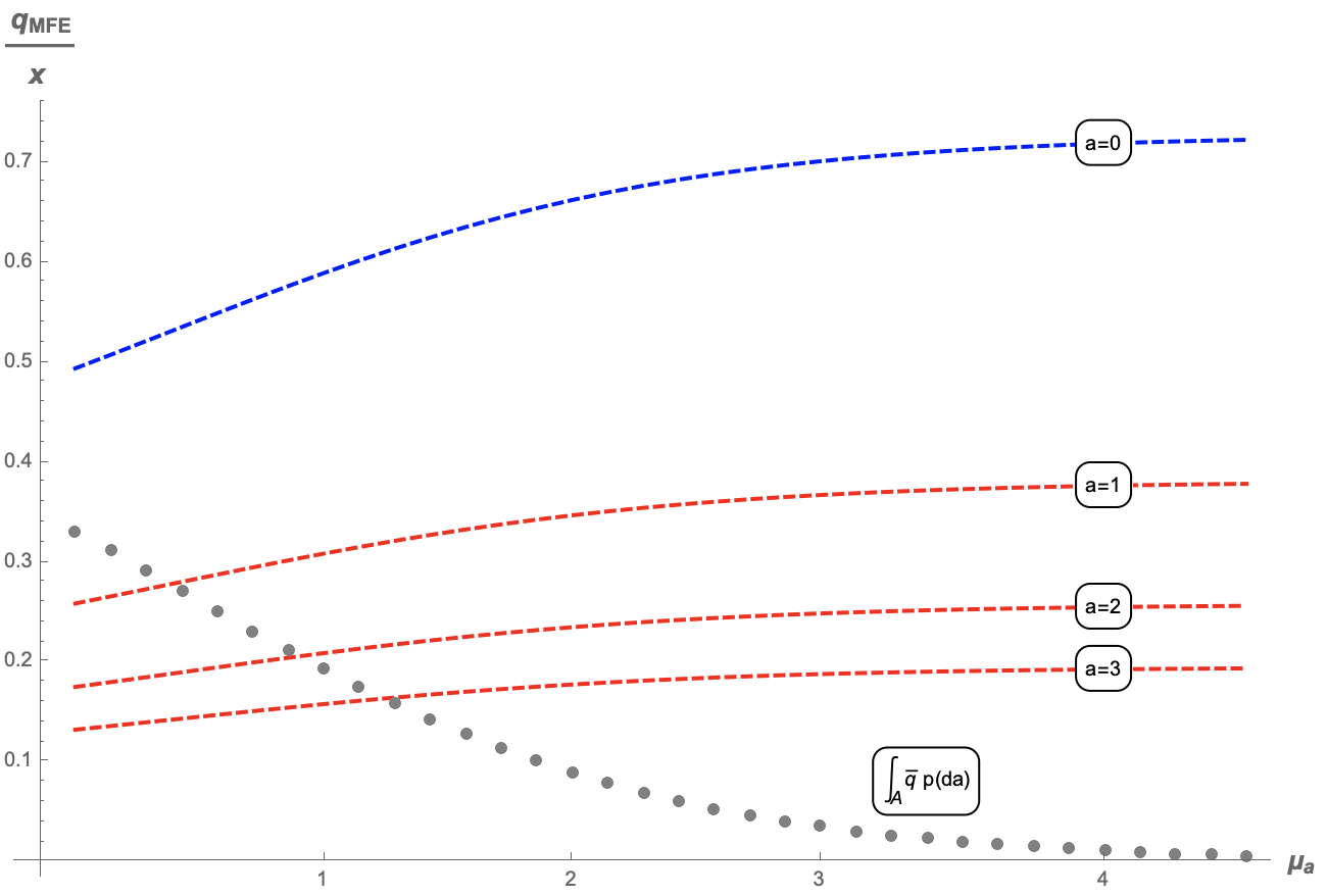
Figure 1: Impact of population and individual ATR beliefs. Dashed lines: equilibrium individual forest consumption rates $q^{MFE}/x$, for different levels of ATR adherence, as the average adherence in the population increases. Dotted line: mean forest consumption rate $\int_{A}\bar{q}p(da)$. Model parameters: $\eta=1.3,\gamma=1.2,\mu=0.4,\sigma=0.05,\rho=0.05$. Beliefs distribution: $\exp N(\mu_{a},0.5)$.

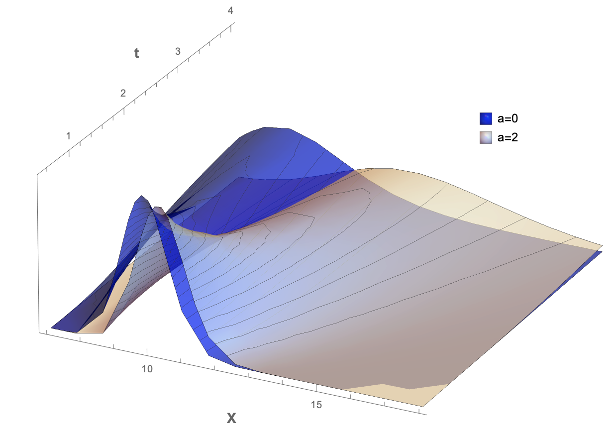
Figure 2: Individual transition density $p^{i}(x,t)$ of equilibrium individual forest cover for two increasing levels of ATR adherence. Model parameters: $\mu=0.3,\sigma=0.2,\eta=3,\gamma=2,\rho=0.05,x_{0}=10,\mu_{a}=1,\sigma_{a}=1$. Time starts at 0.5 for visual clarity.

3.1 Equilibrium Characteristics

Having established the optimal consumption policy, it is a key question to study what is the effect on the deforestation rate of an increase in individual ATR adherence. Furthermore, We also study what is the effect on individual behavior of a change in the beliefs distribution in the population. Let $\mu_{a}$ be a parameter (or a combination of parameters) that regulates the first-order stochastic dominance between different parametrizations of the beliefs distribution, i.e.

$$\mu_{a}\text{ s.t. }\frac{d}{d\mu_{a}}\int_{A}a\times p_{0}^{(\mu_{a})}(da)>0.$$ (11)

One such choice would be the mean $m$ of a Gaussian distribution for the log-normal density $\exp N(m,s^{2})$. As the spatial distribution of the forest cover depends on the distribution of ATR beliefs in the population, we interpret the impact of global/population beliefs as peer effects. We can then state the following Proposition:

Proposition 2. An increase in individual ATR adherence always yields a decrease in the grid-level deforestation rate:

$$\frac{d}{da}\left(\frac{q^{MFE}}{X_{t}}\right)\leq 0.$$ (12)

Furthermore, let $\mu_{a}$ be a parameter in the beliefs distribution such that (11) holds. Then we have the following result:

$$\frac{d}{d\mu_{a}}\left(\frac{q^{MFE}}{X_{t}}\right) \geq 0,$$ (13)

$$\lim_{a\to\infty}\frac{d}{d\mu_{a}}\left(\frac{q^{MFE}}{X_{t}}\right) = 0,$$

which implies that an increase in the average ATR adherence, ceteris paribus, increases individual extraction, and that peer effects are dampened by individual adherence.

Proof: See Appendix C.

To illustrate the equilibrium characteristics, we take as an example that ATR beliefs are log-normally distributed, i.e. $p(a)=\exp N(\mu_{a},\sigma^{2}_{a})\in[0,\infty)$. As discussed in Proposition 2 Figure 1 shows how a decrease in the average adherence in the population $\mu_{a}$ causes an increase in the average forest consumption, as shown by the dotted line. This in turn generates a scarcity of resource (a lower average forest cover) thus resulting in individuals decreasing their consumption proportional to the value they assign to the average forest cover, parameterized by $\gamma$ , as shown by the dashed lines. Note, how for higher individual belief levels the population adherence effects are dampened. Simultaneously, there exists a direct channel where individual beliefs, akin to a random “initial” draw from the beliefs distribution affect individual/localized forest consumption via (7) in Proposition 1. Figure 1 shows how a higher adherence implies a reduced forest consumption, for any given beliefs distribution within the population. Figure 2 illustrates equation 3 i.e. how the equilibrium transition density for each individual forest cover is affected by different levels of $a$ under a log-normal beliefs distribution $p_{0}(a)=\exp N(\mu_{a},\sigma^{2}_{a})$. One can observe how as time increases the individual/localized forest cover $X^{MF}$ associated with a higher individual adherence $a=2$ generates a thicker right tail than the distribution associated to an individual with no adherence ($a=0$), implying that deforestation is reduced locally as adherence increases, whilst the adherence measure within the population remains unchanged. In Appendix D we discuss the relation between beliefs and risk aversion parameter $\eta$ and the possible modelling choices of $g(a)$.

4 Background & Data

First, we provide historical and contemporary overview to motivate our choice of Benin and why it is an ideal case to examine the link between ATR and environmental outcomes. Then in subsection 4.2 we present the main sources of data used and establish the spatial and temporal unit at which the analysis is conducted. We start by focusing on geo-referenced data on religion as covered by the Demographic and Health Survey (DHS) and then document the high resolution time series data on forest cover using a standardized publicly available satellite-based dataset. Appendix E elaborates on the additional data sources and variables used.

4.1 Dahomey: Cradle of Vodun

If the world of Vodun and the world of the ancestors hold together, then Dahomey will not be broken.

–Barthelemy Adoukonou, 1993

The Republic of Benin is a combination of several distinct historical entities which continue to influence the socio-cultural and political dimensions in the present day. Figure 3 and 4 illustrate the contemporary and historical boundaries of the nation. The north-eastern Borgu and Alibori state historically co-existed under the single kingdom of Borgu. As a northern kingdom it was influenced by its geographical position along the Islamic trade routes and extended across the border into present-day Nigeria and to the Sahel in the north. The north-western Atakora and Donga departments brought together several small, acephalous groups who aligned themselves with Borgu in a northern alliance that persists even today. The south-east of the country, Oueme and Plateau, is mainly composed of Yoruba people, who have historically been influenced by the Oyo Empire and in present times by Nigeria. The remaining departments cover what eventually became, from the early eighteenth century, the hegemonic Kingdom of Dahomey which remains of central importance in contemporary Benin.

Established in the early seventeenth century on the Abomey plateau by the Fon people, Dahomey emerged as a full fledged kingdom in the late eighteenth century after ending its tributary status to the looming Oyo Empire. The Kingdom was defined to a great extent by its role in the Atlantic slave trade and facilitated by its expansionist military strategy. Law (1997) states that an annual average of 3.7% of the population under the military sphere of Dahomey were exported, thus highlighting the singularity of its dependence on and participation in the slave trade (Manning, 2004). This was also reflected in the consistent wars and slave raiding in the neighbouring regions which resulted in a fusion of diverse religious beliefs and practices and led to the development of Vodun: a religion where different natural forces were distributed amongst divinities, resulting in an extraordinary pantheon of specialised deities.

As a state religion, Vodun was closely linked to the entire structure of Dahomey’s monarchy and was at the centre of its political ideology and cause. Within the pantheon, the foundation was the cult of the kings themselves and although not himself a god, the king had a sacred role, originating from the royal cult of ancestors (Claffey, 2007). Therefore, as a state, Dahomey combined aspects of caesaropapism and theocracy with absolute monarchy. Moreover, in terms of Christianity Dahomey had the reputation of being defiant to the point of being almost impenetrable (Dupuis, 1998). The constant efforts to resist evangelization is most evident in the fact that prior to colonisation most missionary efforts could not move beyond the port cities. On the contrary, the neighbouring regions of the Kingdom were embracing Christianity. This was especially true for the Yoruba hinterland as the destruction of the Old Oyo Kingdom and the presence of a significant number of established missionary posts led to a remarkable rise in Christianity while Vodun continued to flourish under Dahomey (Vaughan, 2016).

In the nineteenth and twentieth centuries, under colonial rule and the subsequent post independence Marxist-Leninist dictatorship under Mathieu Kérékou, Vodun and other ATR in Benin were marginalized. In 1976, as a part of the sweeping modernization scheme, the Kérékou regime established antiwitchcraft laws (Kahn, 2011). The risk of persecution and intimidation led to a sharp decline in self-reported ATR adherents and a promotion of Christianity and Islam. After the dismantling of the dictatorship in 1991, the new democratic leadership promoted traditional religions as part of a new Béninois national identity and Vodun was officially recognized as a religion within the constitution (Tall, 1995; Stoop et al., 2019). In 1992, the president declared Ouidah’92, a festival for embracing all ATR within the country, which continues to be celebrated today. The unique revival and acceptance of ATR in Benin allows one to safely surmise that self-reported ATR adherence in Benin is a reasonably good proxy for ATR beliefs.

Within the context of an environmental profile, Benin is located in the Guinean forest-savanna mosaic, an important habitat for biodiversity. Between 2005 and 2015 the country’s forest cover dropped drastically by 22% (from 7.6 to 6 million hectares) and sustained a deforestation rate of 2.2 percent per year. According to World Bank (2020) forest ecosystems in the country remain vastly underutilized. Aside from providing key ecosystem services (clean water, controlling soil erosion and carbon sequestration) and representing a means for food security and poverty alleviation; forests in Benin also serve as a place for social, cultural and religious activities. This is especially true for Vodun adherents, the majority traditional religion in the country, who consider forests the place of communion with the gods and sanctuary for initiations (Kokou and Sokpon, 2006; Juhé-Beaulaton, 2010). Landry (2020) emphasises that forests lie at the heart of Vodun and are a place of power and the primary lens through which adherents experience the spirit world. Therefore, the forest is symbolically and ontologically central to their religious worldviews. For example, in Forêt Sacrée de Kpasseeè (Sacred Forest of Kpasse), located in Ouidah, the followers care for the forest, understanding that they are caring for their ancestors, whose spirits are reincarnated into Loko trees (Iroko). Although no official database exists, the Government of Benin estimates that the country has about 3000 sacred forests and groves covering 0.16 percent of the national territory. Benin is the only country in Africa that has implemented a national legislation aiming to recognize sacred natural sites as a category of Benin’s protected areas to maintain important ecological clusters.

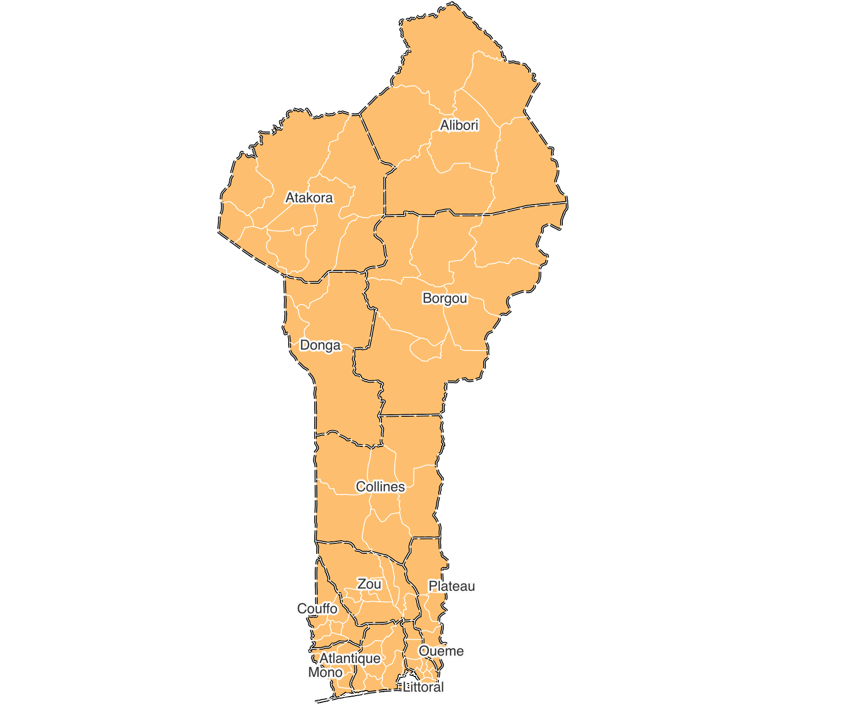
Figure 3: Administrative division levels one and two of Benin. In 1999, the previous six states were each split into two halves, forming the current 12 states (thick lines) and 77 communes (thin lines). Borgu (Alibori & Borgou), Atakora ( Donga & Atakora), Zou (Collines & Zou), Mono (Couffo & Mono), Atlantique (Atlantique & Littoral) and Oueme (Oueme & Plateau).

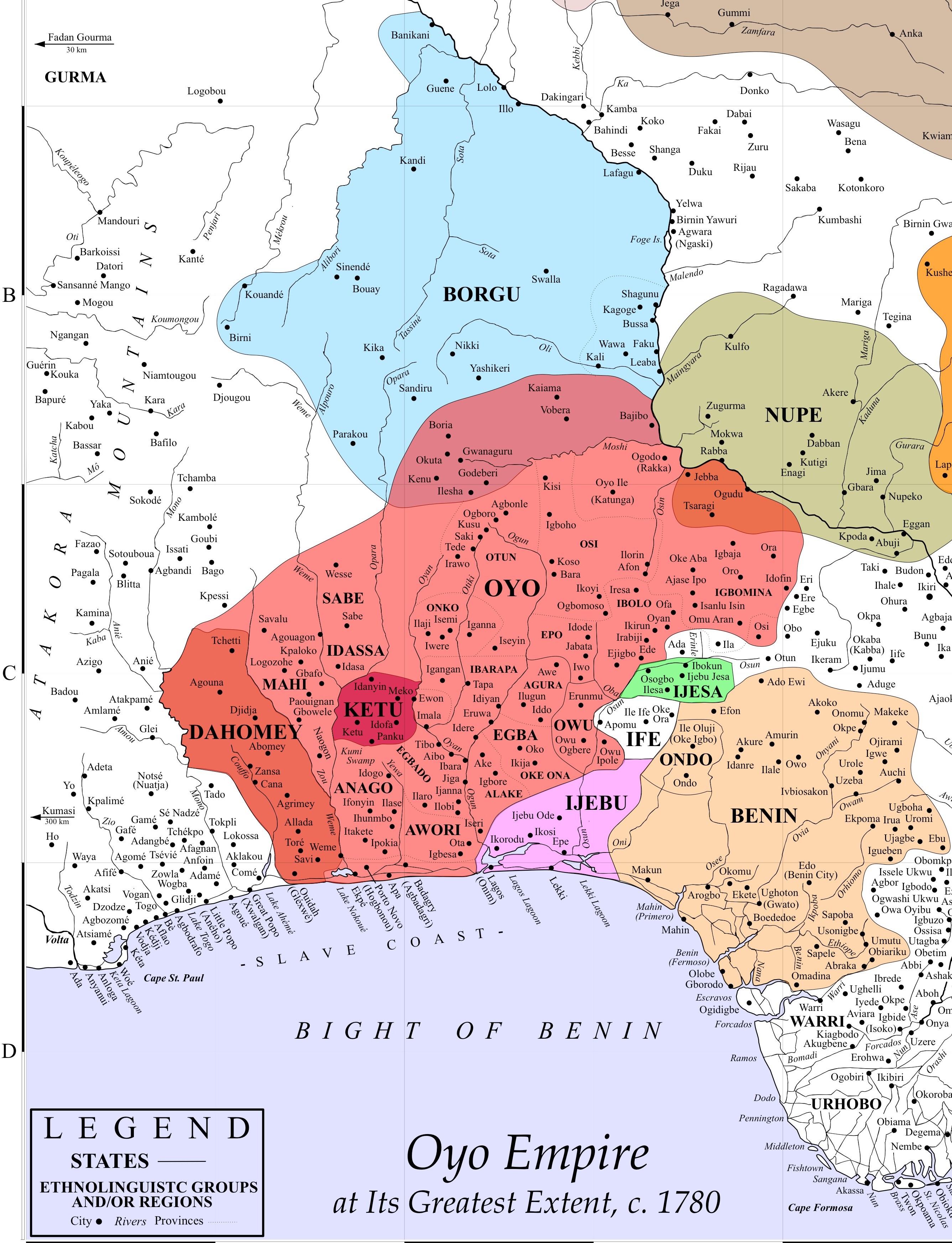
Figure 4: Bight of Benin: Dahomey, Oyo, Borgu and neighbouring kingdoms, 1780. The Kingdom of Benin is not to be confused with modern Republic of Benin. Today the former refers to Benin city in Nigeria and Dahomey refers to the nation state Benin. Source: Lovejoy (2013)

4.2 Data

4.2.1 Religion

We use data from four waves of DHS in Benin, conducted in 1996, 2001, 2012, and 2017. All waves are nationally representative, covering twelve states (administrative division level one) of Benin, and geographic stratification was based on survey clusters, corresponding to villages in rural areas and city blocks in urban areas. Given the cross-sectional nature of the surveys (clusters are not repeated), we construct a grid with cell area corresponding to 10 kms $\times$ 10 kms, over the extent of Benin’s national boundary. Matching the DHS cluster’s GPS coordinates within the grid-cells, we create an unbalanced panel of 479 cells and four time periods (Figure F.1). The empirical analysis is done on this 10 kms $\times$ 10 kms grid-cell resolution. On average, each cell contains 127 individuals. DHS provides detailed information on individual and household socio-demographic characteristics, including religion. Waves 1996 and 2001 have a single category representing Traditional religions, whereas the remaining waves make a distinction between Vodun and other traditional religions. For our analysis, we use ATR to encapsulate both categories, allowing comparability across the surveys. Utilizing the information on self reported religion, we construct a measure of ATR adherence by calculating the percentage share of the individuals in the grid cell that follow ATR. This variable is in essence measuring the ATR market density in each cell (Gruber, 2005).

Turning to descriptive evidence, Figure F.2 presents the evolution of ATR adherence over the 12 states and time. The immediate observation is that the south of Benin has, on average, a higher percentage of ATR adherence, which is consistent with the historical background due to the role played by the Kingdom of Dahomey. In the northern part of the country the only department which has a significant proportion of ATR followers is Atakora, which borders Togo and Burkina Faso. This may be due to the Tammari (Somba) people who continue to practice traditional religions (Blier, 1994). The second observation is that majority of the states show a declining trend, which is also reflected at the national level and for the region of West Africa in Figure F.3. Turning to the spatial variation, Figure 3(a) shows the distribution of all the grid cells by the percentage of ATR adherence over time. One can observe the similar declining trend as the probability of grid cells with more than 50% of ATR adherence fell notably between 1996 and 2016. We also construct religious and ethnic fractionalization indices by grid cells, described in appendix E. Plotting their spatial variation in Figure 3(b) and 3(c) provides an interesting insight into the ethnic and religious landscape of Benin. The ethnic fractionalization distribution is bimodal, an indicator of the north-south division as south is primarily dominated by two large ethnic groups: Fon and Yoruba while the north has more diversity. The religious fractionalization index is striking and consistent across years and in line with the fact that Benin is a country with one of the world’s highest religious diversity index (Pew Research Center, 2014).

4.2.2 Forest Cover

For spatially explicit environmental data we rely on NASA’s Making Earth System Data Records for Use in Research Environments (MEaSUREs) Vegetation Continuous Fields product created by Song et al., 2018. The data provides annual global fractional vegetation cover (FVC) for the time period 1982 - 2016 consisting of tree canopy (TC) cover ($\geq 5$ metres in height), short vegetation (SV) cover and bare ground (BG) cover, at $0.05^{\circ}\times 0.05^{\circ}$ spatial resolution (approximately 5.6 km $\times$ 5.6 km). For each year, every land pixel is characterized by its percentage cover of TC, SV and BG, representing the vegetation composition at the time of the local peak growing season. FVC is a primary means for measuring global forest cover change and is a key parameter for a variety of environmental and climate-related applications. The dataset is derived from a bagged linear model algorithm using Long Term Data Record (LTDR version 4) compiled from Advanced Very High Resolution Radiometer (AVHRR) observations.

As year-to-year changes in forest cover can be volatile, for the main outcome variable we study the average annual change in forest cover over longer time scales. For the instrumental variable strategy, we exploit the temporal dimension of the FVC dataset and in order to combine it with the DHS panel we aggregate the percentage of tree canopy cover in each 10 kms $\times$ 10 kms grid cell $i$ and then calculate the five year average annual change in forest cover as follows:

$$\Delta\text{Cover}^{5y}_{it} =\frac{1}{5}\sum_{t-4}^{t}\Delta\text{Cover}_{it}$$

$$\Delta\text{Cover}_{it} =\text{Tree Cover}_{it}-\text{Tree Cover}_{it-1}$$ (14)

Figure F.5 illustrates the spatial distribution of $\Delta\text{Cover}^{5y}_{it}$ for 1996 and 2016 which distinctly highlights the unsustainable rates of deforestation, especially in the northern region. Similar to the rest of SSA, the main driver of deforestation in Benin is associated with land use change due to extensive shifting agriculture followed by fuelwood and charcoal production, urban expansion, and illegal hunting. Figure F.6 highlights the stark difference in population density between the north and the south but despite low population density, the northern states of Benin are experiencing a high forest cover loss. According to the World Bank (2020), this is linked to agricultural migration as farmers are abandoning degraded areas in search of fertile soils. Figure 3(d) provides the kernel density estimated distribution of grid cells for a key climatic variable: the Palmer Drought Severity Index (PDSI). It is used to quantify long-term drought that has affected a region for several months. The value zero refers to normal and negative numbers refer to the level of dryness. For example, a moderate drought is -2 while conditions of extreme drought start at -4. One can observe a steady move toward increased droughts over time along with variation in intensity across grid cells.

For spatial RDD, while we lose the temporal variation we exploit the full granularity of the FVC dataset by using the original spatial resolution and study over three timescales: 5, 10 and 15 years average annual change in forest cover in each 5.6 kms $\times$ 5.6 kms grid cell $j$, over the most recent period covered in the data (2012-2016, 2007-2016, 2002-2016). This is calculated as follows:

$$\Delta\text{Cover}^{ky}_{j} =\frac{1}{k}\sum_{2016-k-1}^{2016}\Delta\text{Cover}_{jt},\ \ k\in\{5,10,15\}$$

$$\Delta\text{Cover}_{jt} =\text{Tree Cover}_{jt}-\text{Tree Cover}_{jt-1}$$ (15)

5 Empirical Evidence

5.1 OLS and Instrumental Variable Strategy

To identify the effect of ATR on forest cover dynamics we begin by a baseline OLS estimation using the following specification:

$$\Delta\text{Cover}^{5y}_{icdt} =\beta\text{ATR}_{it}+\boldsymbol{\theta}\textbf{X}_{it}+\sum_{c}\text{commune}_{c}\times t+\alpha_{i}+\phi_{dt}+\epsilon_{icdt}$$ (16)

where $\Delta\text{Cover}^{5y}_{icdt}$ is the 5 year average annual change in forest cover for grid cell $i$ of resolution 10 kms $\times$ 10 kms in commune $c$ within state $d$ for a given year $t$. $\text{ATR}_{it}$ is the percentage of individuals who are adherents of African Traditional Religions within cell $i$. To isolate the effect of ATR and to control for factors that maybe correlated with and may affect the change in forest cover, we include $\textbf{X}_{it}$ which is a vector of cell-level geographic, climatic, socio-economic and agricultural controls. These covariates, as summarised in Table F.2, control adequately for differential trends in local conditions and determinants of change in forest cover, that happen to be correlated with ATR adherence. The specification also includes commune (administrative division level two) specific linear time trend denoted by $\sum_{c}\text{commune}_{c}\times t$ and a rich set of fixed-effects: $\alpha_{i}$ grid cell fixed effects which absorb all differences in the change in forest cover across cells due to time-invariant characteristics, and $\phi_{dt}$ state-by-year fixed effects which capture non-linear time trends specific to each of the twelve states across Benin. The main coefficient of interest is $\beta$ which is the effect of ATR adherence on five years average annual change in forest cover. The standard errors are robust and clustered at the commune level.

Conditioning on observables does not necessarily control for all sources of potential correlation between ATR adherence and the error term. Therefore (16) still poses the classical omitted-variable bias. More specifically, it may very well be the case that due to the importance of forests within the ATR cosmology adherents may have a preference to settle in areas with pre-existing high forest cover or precedent pro-environmental preferences may influence the selection into ATR thus influencing both ATR adherence and forest cover change. This leads to the main issue in the identification of (16): the potential non-random allocation of ATR adherents across cells. To mitigate the bias, we rely on an instrumental variable approach. We exploit the spatial variation regarding the grid cell’s proximity to the Nigerian border. For the first-stage equation, we use as an instrument for ATR adherence the interaction between the log of the distance from the Nigerian border and a linear time (year) trend $t$ that captures the generalized decrease in adherence to traditional religions across Benin:

$$\text{Z}_{it} =\text{log(Dist. from Nigeria)}_{i}\times t$$ (17)

To assess the validity of the identification strategy we first establish relevance by briefly describing Benin and Nigeria’s historical relationship, and subsequently demonstrate exogeneity and exclusion restriction. The two countries have been historically intertwined, with the Kingdom of Dahomey (present day southwest Benin) having been a tributary of the Oyo Empire of Yoruba people (present day southwest Nigeria and southeast Benin) in the early eighteenth century. However, by the nineteenth century Dahomey had asserted its independence and become an important rival of Oyo in the Atlantic slave trade. Moreover, access to important port cities such as Ouidah or Little Popo often required crossing through the Dahomey territory (Lovejoy, 2019). This led to the diffusion of social and cultural practices across kingdoms through their shared interests in trade, and their intermediary position between trans-Atlantic and trans-Saharan commerce.

Vaughan (2016) discusses two important regional movements in the late nineteenth century: First, in 1804 the Fulani (Sokoto) jihad led to the subsequent creation of The Sokoto Caliphate, which became one of the largest states in Africa in the nineteenth century. The rise and influence of this major Muslim reformist movement in contemporary Nigeria’s vast northern region, spread gradually through its northern neighbours including Borgu (present day northeast Benin). Second, a Christian evangelical movement in the Oyo - Yoruba territory in southern Nigeria was propelled by the influential English missionary organization called the Church Missionary Society (CMS). The first major group of Christian missionaries charged with the responsibility of evangelizing arrived in 1842, a period when the British wanted to forestall the growing threat of Dahomey. The success of the CMS missionaries led to a rapid expansion in Christian missions, eventually reaching as far as the Gold Coast and Togoland (Claffey, 2007; Akinwumi, 1999).

These events combined with Nigeria’s prominence in the region, resulted in it influencing the religious makeup and geopolitics of its neighbors. This can also be gauged in the more recent phenomenon of the expansion of Pentecostalism from Nigeria into other West African countries (Obadare, 2018). Thus one can infer that for Benin, where due to the geographical proximity and close historical ties, the distance from present day Nigerian border is indicative of the displacement of traditional religions and adoption of Christianity and Islam. Figure 5 is consistent with this observation as one can note that the southeast and centre of Benin has a dominant proportion of Christian followers: a direct influence of the Yoruba people of southwestern Nigeria embracing Christianity in the second half of the nineteenth century and the subsequent success of the Yoruba Christian church movement (Claffey, 2007). Similarly, the northeastern region of Benin which bordered Hausa-Fulani Muslim Kingdoms to the north and was influenced by the Sokoto Caliphate in the east, continues to be dominated by Islam. Therefore, based on the close historical relationship between the two nations and Nigeria’s significant influence on the religious markets in Benin, the hypothesis is that the further away is the cell from the border, the more likely it is to have a higher proportion of ATR followers and vice-versa.

A unique advantage of using the distance from the Nigerian border as an instrument is that the creation of this border was exogenous to ecological factors and was a consequence of the scramble for Africa. Primarily motivated by political and colonial interests, it was decided by European representatives who had little knowledge of the local geography, with the exception of few coastal areas (Michalopoulos and Papaioannou, 2016). This was especially true for Benin and Nigeria where the border was simply seen as a separation between the English and the French (Asiwaju, 1985). While the location of the Nigerian border was exogenously determined, a potential concern here might be that the distance from the Nigerian border might be correlated with geographical variables (e.g. distance to the coast, elevation, terrain, soil suitability for agriculture) or climatic variables (e.g. rain and temperature) or with the availability of other infrastructure and services (i.e. roads and waterways) or relevant social indicators such as ethnic and religious fractionalization that are known to matter for forest cover change and that might have an independent effect. However, as discussed above we address this by including an exhaustive array of cell level characteristics detailed in Table F.2 and conduct appropriate robustness checks. Therefore, the exclusion restriction for this IV is that - conditional on the included controls - the distance from the border affects only the spatial distribution of ATR and is not correlated with any unobserved local factors that might influence forest cover dynamics.

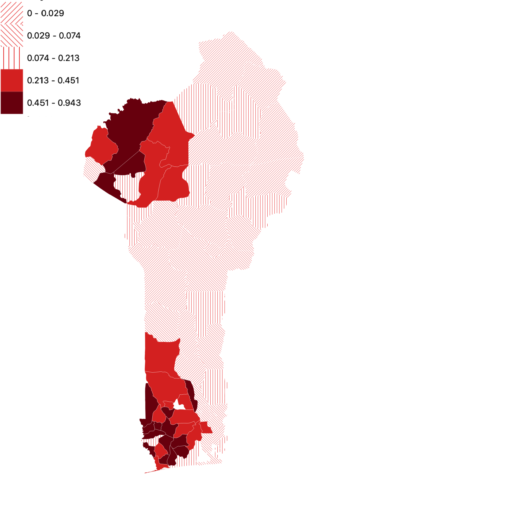
(a) ATR

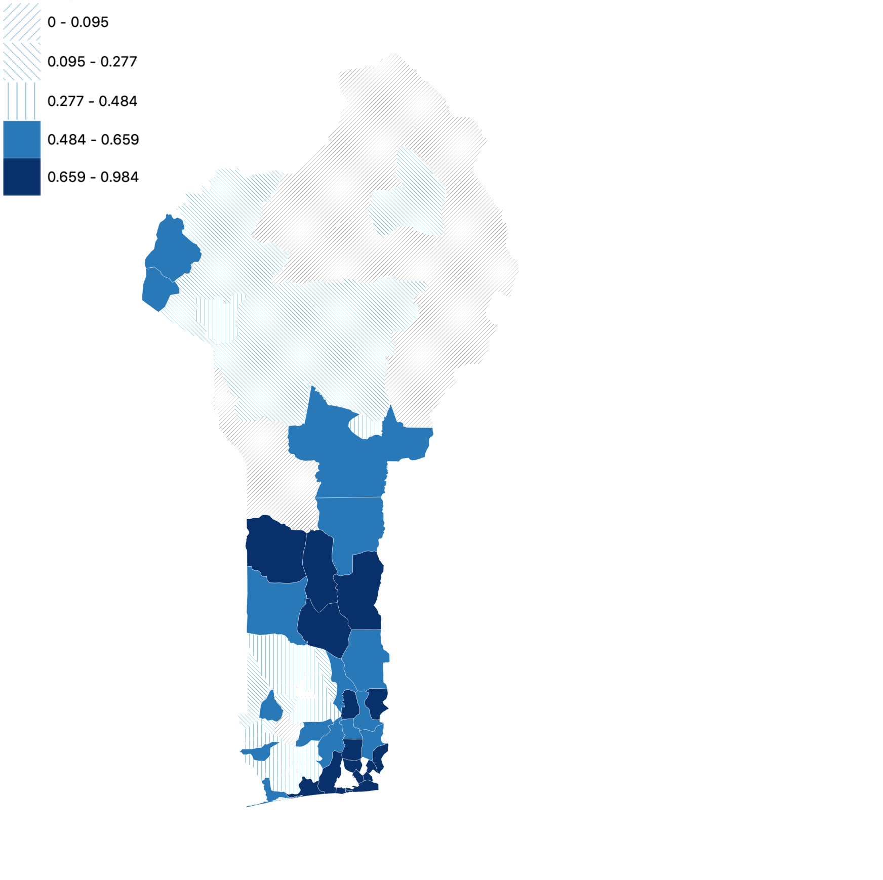
(b) Christianity (all denominations)

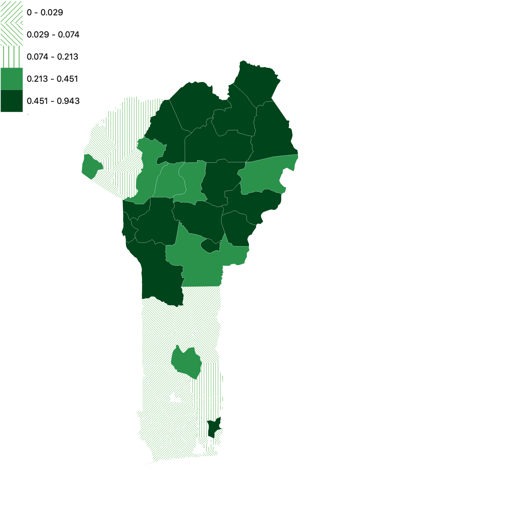
(c) Islam

Figure 5: Spatial distribution of religions in Benin based on 1996 DHS.

5.1.1 Results

Table 1 presents the results, going from parsimonious to more inclusive specifications. In column (1), we simply regress the five year average annual change in forest cover on ATR adherence with cell and year fixed effects. We find the coefficient to be positive but small and unable to reject the null hypothesis. In column (2), we introduce state $\times$ year fixed effects capturing non-linear time trends across the twelve states, this increases the magnitude of the estimate but continues to not be significant. When controlling for commune specific trends in column (3) we find that the coefficient becomes larger in magnitude and significant, indicating that 1 percentage point increase in ATR adherence is correlated with a 0.014 percentage point positive effect on the 5 year average annual change in forest cover. In column (4) despite including a full set of climatic, geographic, socio-economic and agricultural controls, the coefficient continues to be significant with a slight decrease in magnitude. To probe the robustness of the estimates, we run the specification under every possible combination of different groups of control variables. Figure F.7 reports coefficient estimates for each of these 512 models. The majority of coefficient estimates on ATR adherence are statistically significant at 5 and 1 percent level, including the most demanding and most precisely estimated specification reported in column (4). Moreover, the coefficient estimates are relatively stable.

Tackling the endogeneity concerns with IV, column (5) reports the first-stage estimate from equation (17) showing a strong and significant relationship between the instrument and ATR adherence. Consistent with the hypothesis discussed, we find that farther distances from the Nigerian border are associated with higher adherence to ATR. The Kleibergen-Paap F statistic of 12 and the confidence interval proposed by Chernozhukov and Hansen (2008), robust to both weak instruments and heteroskedasticity and/or autocorrelation, give further confidence that the instrument is sufficiently relevant. Column (6) presents the IV coefficient estimate which corroborates the OLS results: a 1 percentage point increase in ATR adherence in a grid cell $i$ is associated with a 0.09 percentage point positive effect on the five year average annual change in forest cover. Put differently, a 1 standard deviation increase in ATR adherence has a 0.43 standard deviation positive impact on the forest change outcome. We observe that the IV estimate is about 2 times larger than the OLS in column (4). This maybe to an extent because of attenuation bias as religious syncretism is common in Benin. Additionally, the IV estimate is capturing the average treatment effect driven by the variation in the spatial distribution of ATR caused only by the instrument.

Spatially explicit estimation along with an instrument based on geography introduces a high potential for spatial correlation in the data. Therefore, in the appendix Table F.1 we show the robustness of both OLS and IV estimates when accounting for potential dependence based on spatial proximity by using Conley (1999) standard errors with a cutoff of 150 kms. To further test the sensitivity of the results to omitted variable bias, we follow Oster (2019) which is based on earlier work by Altonji et al. (2005). Under the assumption that selection on the observed covariates is proportional to selection on unobservables, Oster (2019) constructs an estimator for the degree of selection on unobservables relative to observables ($\delta$) needed for the true effect of the treatment variable to be a statistical null. Following the recommendation of using 1.3 times the $R^{2}$ value of the most extensive specification, we find $\delta=2.95$ suggesting that a very high level of selection on unobservables is required for the non-zero estimates to represent a spurious correlation.

Although we provide evidence for the validity of the instrument, we recognize that the requirement of perfect exogeneity is a knife requirement that, strictly speaking, is unlikely to hold exactly. To gain a sense of the robustness of the IV estimates, we relax the exclusion restriction and examine the bounds we are able to place on the true effect of ATR adherence on forest cover change while deviating from perfect exogeneity. Following Conley et al. (2012), the sensitivity analysis assumes that $\text{log(Dist. from Nigeria)}_{i}\times t$ does in fact appear in (16):

$$\Delta\text{Cover}^{5y}_{icdt} =\beta\text{ATR}_{it}+\tilde{\gamma}\text{log(Dist. from Nigeria)}_{i}\times t$$

$$+\boldsymbol{\theta}\textbf{X}_{it}+\sum_{c}\text{commune}_{c}\times t+\alpha_{i}+\phi_{dt}+\epsilon_{icdt}$$

The idea is intuitive. If we were to know the true value of $\tilde{\gamma}$, it would be straightforward to estimate the above equation by 2SLS but we do not know the true value, therefore, Conley et al. (2012) tackle this problem by making assumptions on the support of $\tilde{\gamma}$ and subsequently estimate the confidence interval for $\beta$ (the coefficient of interest). We calculate this interval using the union of confidence intervals approach. This method is based on the assumption that the researcher can specify the support of $\tilde{\gamma}$, but yields the most conservative interval estimates of $\beta$. An intuitive approach is to link this support to $\beta$, since the magnitude of the coefficient of interest provides a natural frame of reference. A common strategy is to use a $\tilde{\gamma}$ of .3, which limits $\tilde{\gamma}$ to no more than 30% of the value of $\beta$ estimated from the IV regression. Yet for the purposes of this study, we take a conservative approach and allow for a $\tilde{\gamma}$ of up to 100% of the value of $\beta$. We thus choose $\tilde{\gamma}$ from the symmetric support of $[-\tilde{\gamma}\beta$,$\tilde{\gamma}\beta]$, where $\tilde{\gamma}=1$, and $\beta$ is the coefficient of interest estimated in column (6) of Table 1. Results are shown in Figure F.8. The dashed lines are the 95% confidence interval bounds for $\beta$ given different magnitudes of $\tilde{\gamma}$ along the x-axis. We find that the interval only includes zero when $\tilde{\gamma}$ is relatively large in magnitude (that is, when it is about 65% of the value of $\beta$).

As a further robustness check, we estimate two additional sets of IV regressions by restricting the sample to the southern departments of Benin where the Kingdom of Dahomey was located and where majority of ATR adherents live even today. See Figure 5. Focusing on the south implies that the likelihood of ATR self-selection occurring is even lower as the inheritance of Vodun from the Kingdom still persists. First, in Table F.3 Panel A, we continue to exploit distance from the Nigerian border as an instrument. As expected, the first stage results show a significant relationship and the instrument is stronger with a Kleibergen-Paap F statistic of 19.73. Column (2) presents the IV estimate which corroborate with those presented in Table 1, the coefficient is larger in magnitude and we find that a 1 percentage point increase in ATR adherence has a 0.13 percentage point positive impact on the five year average annual change in forest cover.

Second, based on Section 4.1 we utilize the information that Dahomey had persistently resisted evangelization while the neighbouring Nigeria had embraced Christianity. Therefore, a part of the south had significant exposure to ATR and the other to Christianity. Figure F.9 shows the location of all Protestant and Catholic missions in the region in 1924 as reported by Roome (1925). One can observe that while missionaries had managed to establish posts further inland in Nigeria and Togo, this was not the case for Benin. Following a vast literature on exposure to missionaries as a treatment (Nunn et al., 2014; Valencia Caicedo, 2019; Jedwab et al., 2021; Jedwab et al., 2022) we hypothesise that, conditional on the included controls, groups that experienced little to none missionary contact are today more likely to self-identify as ATR. This is in line with Nunn (2010) who found evidence that foreign missionaries altered the religious beliefs on the African continent and that these beliefs persist even today. We use distance from the closest mission post as an instrument. We report the results in Panel B of Table F.3. The first stage results in column (3) are strong and significant showing that farther distances from the missions are associated with a higher ATR adherence. The IV estimate is approximately the same magnitude as in Panel (A) albeit with a weaker significance at ten percent.

Therefore, consistent with the model prediction in Proposition 2 equation 12 the results show that ATR beliefs at a localized cell level have a positive impact on forest cover change and that this relationship is in fact causal and robust. We now explore the externality arising from the population ATR adherence on cell level forest dynamics. To do so we estimate the OLS specification (16) by dropping state-by-year fixed effects and introducing an additional explanatory variable capturing the global average adherence in the population. The global adherence is what the individual agent incorporates into her optimization, therefore, it is important to define what one means by global empirically. We take two geographical limitations to capture the population adherence: average ATR adherence at the state level and the average defined over 50 kms buffer from the centroid of the grid cells. It maybe that that the cell $i$ incorporates the average beliefs defined by an administrative border such as a state or it may simply be the geographical proximity captured by the buffer.

Table F.4 columns (1) and (2) show the OLS results and columns (3) and (4) instrument the localized ATR adherence in 10 kms $\times$ 10 kms grid cells by distance to Nigerian border. We find that while the local ATR adherence for cell $i$ continues to have a positive and significant effect with magnitudes similar to columns (4) & (6) in Table 1, the global adherence for both variables has a negative and significant effect on the five year average annual change in forest cover. Consistent with the model prediction we find that when the average adherence in the reference population increases it has a negative effect on the cell level forest cover change. Moreover, the model predicts that this effect is dampened by localized beliefs and therefore to explore this we introduce an interaction term in columns (5) & (6) and show the marginal effects in Figure 6. We find that the impact of the global ATR adherence is only significant at low levels of local ATR adherence and becomes insignificant at higher levels.

Table 1: OLS & instrumental variable estimates

					First Stage	2SLS
	$\Delta\text{Cover}^{5y}_{icdt}$				ATRit	$\Delta\text{Cover}^{5y}_{icdt}$
	(1)	(2)	(3)	(4)	(5)	(6)
ATRit	0.005	0.011	0.014∗∗∗	0.013∗∗		0.092∗∗
	(0.008)	(0.008)	(0.005)	(0.005)		(0.035)
log(Dist. from Nigeria)i					2.489∗∗
$\times$					(0.776)
time
Observations	905	905	905	887	887	887
Cell FE	✓	✓	✓	✓	✓	✓
Year FE	✓	✓	✓	✓	✓	✓
State $\times$ Year FE		✓	✓	✓	✓	✓
Commune time trend			✓	✓	✓	✓
Climatic controls				✓	✓	✓
Geographic controls				✓	✓	✓
Socio-Economic Controls				✓	✓	✓
Agricultural Controls				✓	✓	✓
K-P F Statistic					12.12
Robust Confidence Interval						[0.02, 0.15]

• Unit of analysis is 10 kms $\times$ 10 kms grid cell. Robust standard errors clustered at commune level. 95% confidence intervals computed as shown by Chernozhukov and Hansen (2008). Columns (1) to (4) use equation (16). Columns (5) and (6) implement IV approach and first stage uses equation (17). Climatic controls include: precipitation, Palmer Drought Severity Index and minimum and maximum temperature. Geographic controls include elevation, terrain slope class, soil suitability for agriculture, distance to coast, distance to primary and secondary roads, distance to waterways, distance to protected areas, latitude and longitude - these are interacted with a linear time trend. Socio-economic controls include population density, nighttime lights luminosity, education, wealth, use of firewood as cooking fuel, religious and ethnic fractionalization per grid-cell. Finally the agricultural controls include area used for harvesting of the major subsistence and cash crops in Benin: maize, yam, cassava, cotton, peanuts and vegetables. ^∗p$<$0.1; ^∗∗p$<$0.05; ^∗∗∗p$<$0.01.

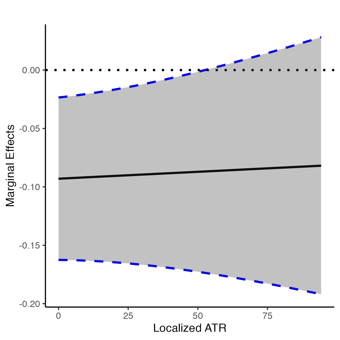
(a) Global adherence: State ATR

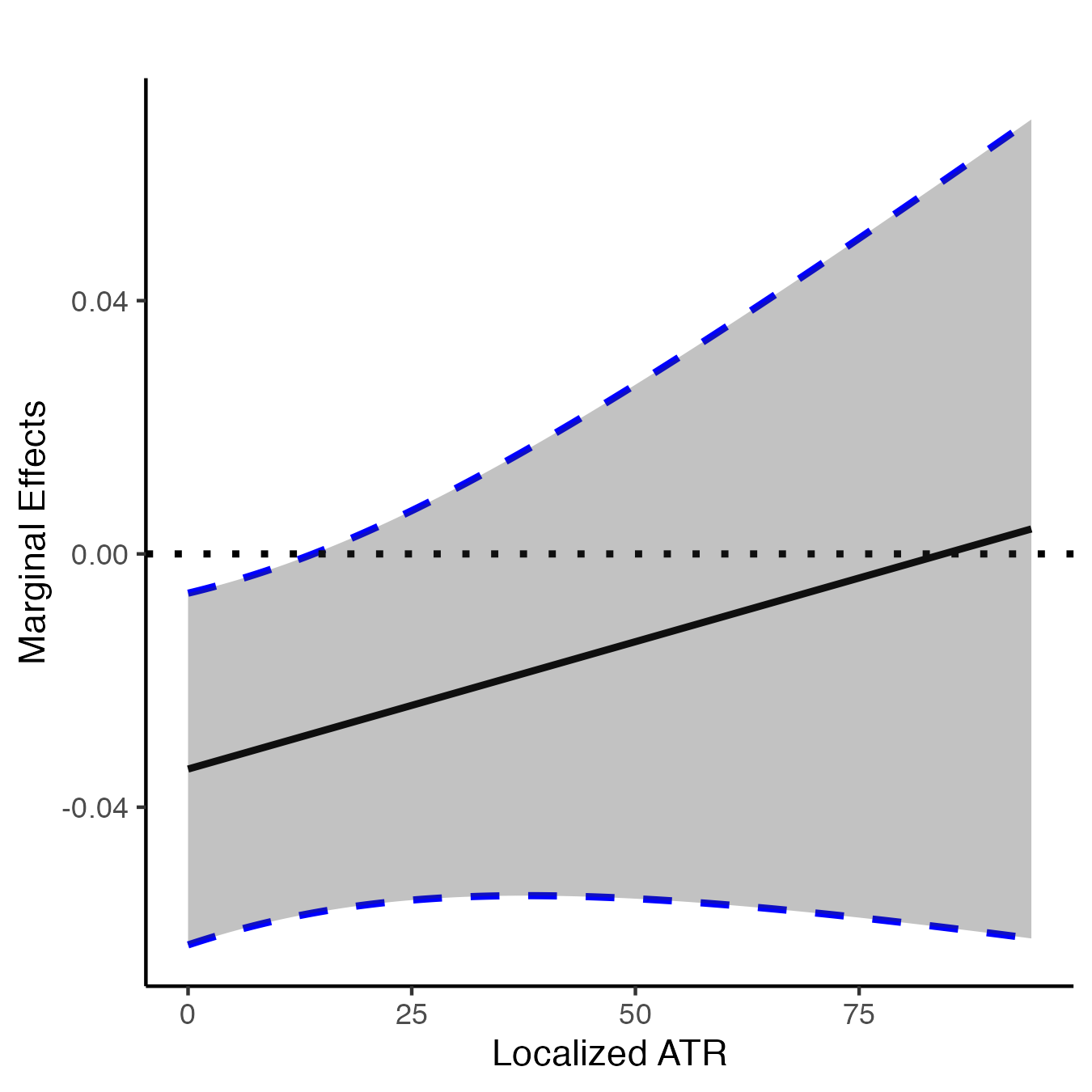
(b) Global adherence: ATR${}^{50kms\;\text{buffer}}$

Figure 6: Marginal effects of global ATR adherence on forest cover change varying with localized levels of ATR adherence at 10 kms $\times$ 10 kms grid cell. Results from Table F.4 columns (5) & (6). 95% confidence intervals.

5.2 Spatial Regression Discontinuity Design

As an alternate strategy for identification, we exploit the historical boundaries of the Kingdom of Dahomey as a spatial discontinuity. As detailed in Section 4.1, Dahomey was unique in its single minded resistance toward evangelization and Vodun was a state religion and an important aspect of Dahomey’s monarchy. According to Claffey (2007) Vodun spread to all corners of the Dahomey society and was a great lattice upon which society and state were constructed and maintained. Based on Weber (1922)’s stylized theory of legitimization suggesting that one of the ways rulers can legitimize their power is through religion, Bentzen and Gokmen (2022) show that stratified societies that used religion for legitimacy in their past are more likely experience persistence of religion today. Although Vodun had high gods they were primarily otiose but the central role played by the royal cult of ancestors put them at the top of the pantheon of gods and divinities.

Using regression discontinuity design, we compare nearby grid cells that belonged to Dahomey to those just outside the Kingdom, in order to investigate the impact on contemporary forest cover change. Figure F.10 represents the boundaries of Dahomey at its peak in the nineteenth century and Figure 7 shows the historical boundaries overlaid on present day borders with the relevant boundary being the northern border, indicated with a solid red line. This boundary forms a multi-dimensional discontinuity in longitude-latitude space, and regression takes the form:

$$\Delta\text{Cover}^{ky}_{jb} =\zeta\text{Dahomey}_{j}+f\text{(geographic location${}_{j}$)}$$

$$+\boldsymbol{\kappa}\textbf{Z}_{j}+\Omega_{b}+\epsilon_{jb}$$ (18)

where $\Delta\text{Cover}^{ky}_{jb}$ is the $k=5,\;10,\;15$ years average annual change in forest cover in grid cell $j$ of spatial resolution 5.6 kms $\times$ 5.6 kms. $\text{Dahomey}_{j}$ is an indicator equal to 1 if the cell $j$ falls within the boundaries of Dahomey and equal to zero otherwise. $f\text{(geographic location${}_{j}$)}$ is the RD polynomial, which controls for smooth functions of the geographic location of grid cell $j$. The term $\Omega_{b}$ represents boundary segment fixed effects that ensures we am comparing grid cells that are within the same segment of the border. Finally, $\textbf{Z}_{j}$ is a vector of two cell-level controls (i) agro-ecological zones and (ii) due to the major role played by Dahomey in the Atlantic slave trade, we include in all regressions the distance of grid cell $j$ from the coast to explicitly control for the direct and indirect effects of past exposure to slavery as the north of Benin was a common slave raiding region for several regional kingdoms. The baseline specification limits the sample to grid cells within 30 kilometers of the threshold. Following Gelman and Imbens (2019), we use a local linear and quadratic RD polynomial in latitude and longitude and document robustness to a wide variety of different bandwidths. The main coefficient of interest is $\zeta$ which captures the local average difference in the $k$ years average annual change in forest cover between grid cells that fall within and outside the Kingdom.

The key identifying assumption is that all relevant factors besides treatment vary smoothly at the boundary. That is, letting $\tau_{1}$ and $\tau_{0}$ denote potential outcomes under treatment and control, $x$ denote longitude, and $y$ denote latitude, identification requires that $\operatorname{E}[\tau_{1}|x,y]$ and $\operatorname{E}[\tau_{0}|x,y]$ are continuous at the discontinuity threshold (Dell et al., 2018). This assumption is needed for observations located just across the Dahomey boundary within the Kingdom to be an appropriate counterfactual for observations located just outside the Kingdom. A crucial concern for identification is that the Kingdom of Dahomey expanded in a strategic manner for certain characteristics (fertile lands, advantageous terrain etc.) that could also affect the ecological dynamics. Section 4.1 provides historical evidence that after the initial establishment of Dahomey on the Abomey Plateau, the subsequent expansion policy was primarily motivated by aggressive military and political strategy with the aim of profiting from the salve trade and not environmental factors. An alternative argument would be that the areas within Dahomey had a denser baseline forest cover to start with and persistence of the initial stock has provided an ecological advantage. To control for this, ideally we would like to have early seventeenth century historical forest or vegetation maps to conduct the appropriate balance check before the establishment of what became known as The Kingdom of Dahomey, however, this data is unavailable. Therefore, as a proxy we use 1600 AD historical land use estimates on cropland and grazing, provided by the History Database of the Global Environment (Klein Goldewijk et al., 2017).

To assess the plausibility of the identification assumption, Table F.5 examines a variety of relevant geographic (elevation, slope, distance to roads and waterways), climatic (precipitation and temperature), demographic (population density and nighttime lights), agricultural (crop soil suitability) and pre Dahomey land use (1600 AD estimates of croplands and grazing) characteristics. Regressions are of the form described in equation (18). We find these to be statistically insignificant, implying the characteristics are smooth (balanced) at the threshold and confirming the validity of the design.

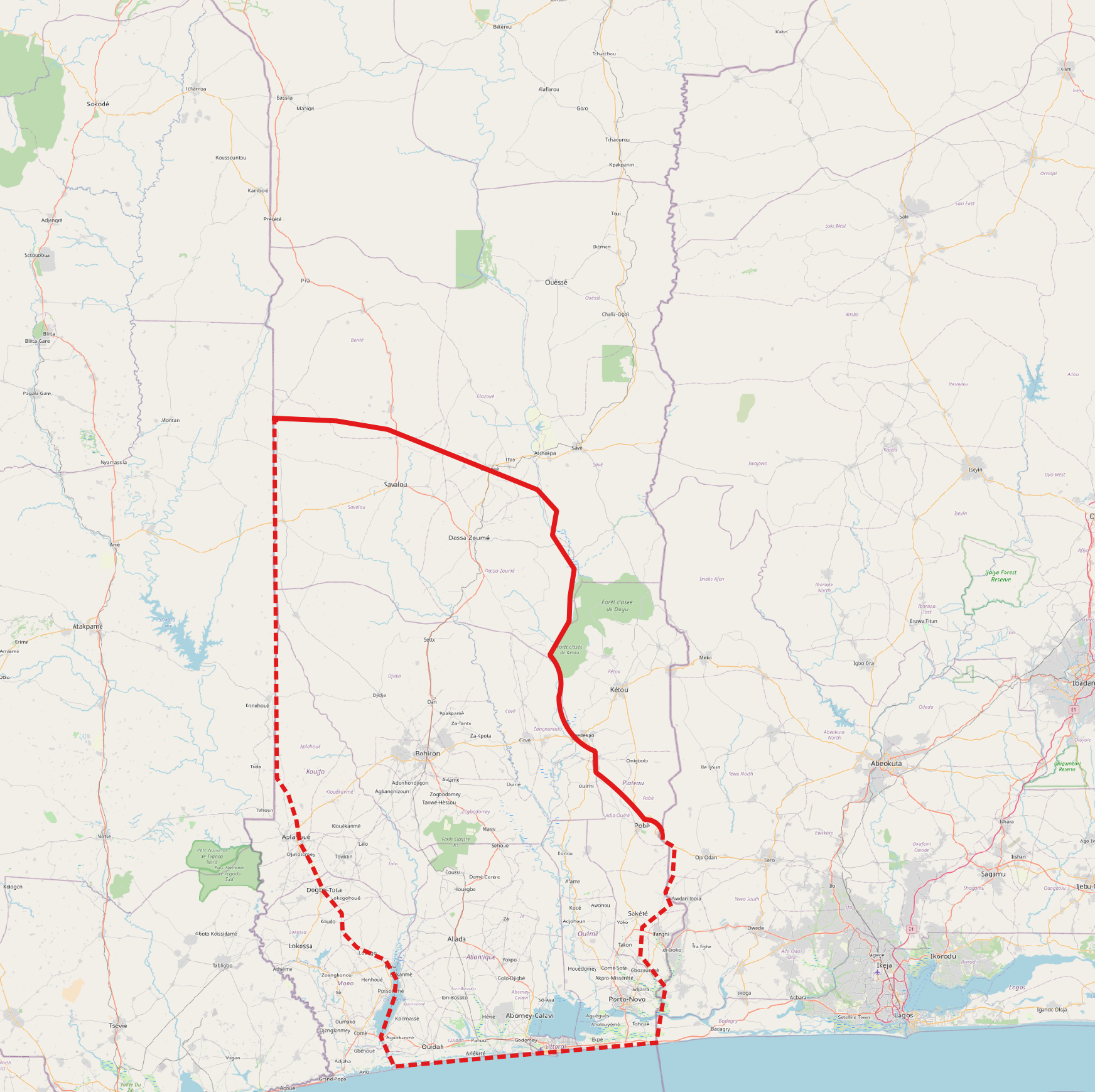
Figure 7: Boundaries of the Kingdom of Dahomey in the nineteenth century. Source: Lovejoy (2019)

5.2.1 Results

As a first pass, we begin with a graphical analysis in Figure 8 which plots the binned outcome means against the distance to the documented border of the Kingdom of Dahomey. One can observe a positive jump at the cutoff in Figures 8(b) and 8(c) indicating that the 10 and 15 years average annual change in forest cover is positive for cells which fall within Dahomey than in those which are right outside the border. Table 2 reports estimates from equation (18) where the top panel uses a local linear RD polynomial and the bottom panel uses a quadratic RD polynomial. Consistent with Figure 8(a) $\Delta\text{Cover}^{5y}_{jb}$ is not significant but we find the coefficient to have the anticipated positive sign. For both panels in column (2) the point estimates suggest that the 10 years average annual change in forest cover is significant and positive by one-third for the grid cells located within Dahomey. Similarly, the average annual change over 15 years is positive by 0.2 for cells within the historical boundaries of the Kingdom. In the appendix Table F.6 we show the robustness of the estimates when using Conley standard errors with a cut-off window of 50 kms to account for spatial auto-correlation. Additionally, as there is no widely accepted optimal bandwidth for a multidimensional RD we further check the robustness by plotting estimates from equation (18) for different bandwidth values between 10 and 50 kms as shown in Figure F.11. The bandwidth under consideration is denoted on the x-axis and the error bars show 90% confidence intervals. The linear RD polynomial for $\Delta\text{Cover}^{10y}_{jb}$ is highly robust to alternative bandwidth choices. For the others, although the estimates are noisy at the extreme ends, the results hold between bandwidths of 15 kms and 35 kms.

An additional issue is that despite using Conley standard errors, spatial correlation is still a natural concern in persistence and historical studies. Kelly (2021) argues that spatial auto-correlation in these studies often lead to inflated t-statistics that complicate the interpretation of estimated results and kernel standard errors are usually not much larger than uncorrected ones. Kelly (2021) proposes a spatial noise randomization procedure that involves estimating the spatial parameters of the explanatory variable $X$ and simulating noise with the same structure. The significance level of $X$ is the fraction of regressions where the replacement synthetic noise has a more extreme t statistic than the original estimate. Specifically, the null hypothesis is that $X$ has no more explanatory power than spatial noise with a given set of generating parameters. Compared to the cluster and principal component results, these randomized estimates are robust. Table F.8 columns (2) - (4) provide the maximum likelihood estimates of the spatial structure of the orthogonalized explanatory variable $\text{Dahomey}_{j}$ and these are used to generate synthetic noise for the randomized significance level in column (5). Directional $R^{2}$ tells how much of the orthogonalized explanatory variable is explained by spatial trends. The value of 0.039 here suggests that $\text{Dahomey}_{j}$ is not acting as a proxy for any omitted directional trends and (18) is a relatively well specified model. The effective range of 80 kms is where the correlation between locations of the detrended variable has fallen to 0.14 and the spatial structure of 0.8 is high, meaning that most variables lie close to the predicted spatial surface with little idiosyncratic variation. The significant randomized p value in column (5) indicates that we can reject the null that the explanatory power of $\text{Dahomey}_{j}$ is due to spatial noise, thus reassuring us of the validity of results in Table 2.

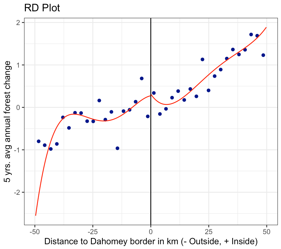
(a) $\Delta\text{Cover}^{5y}_{jb}$

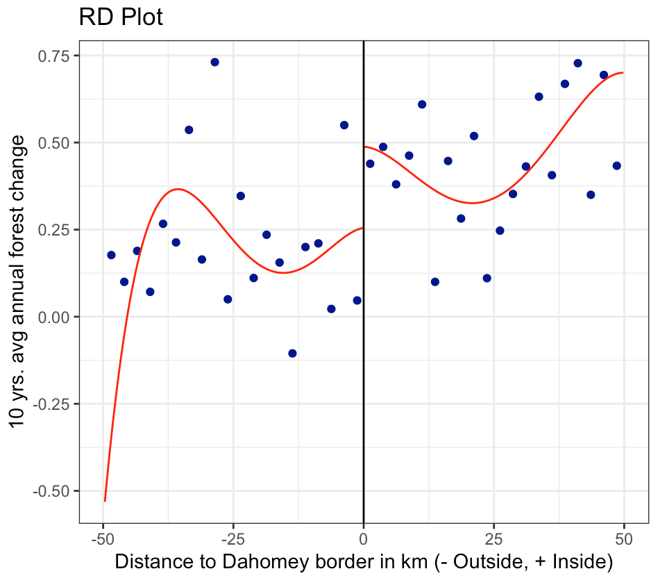
(b) $\Delta\text{Cover}^{10y}_{jb}$

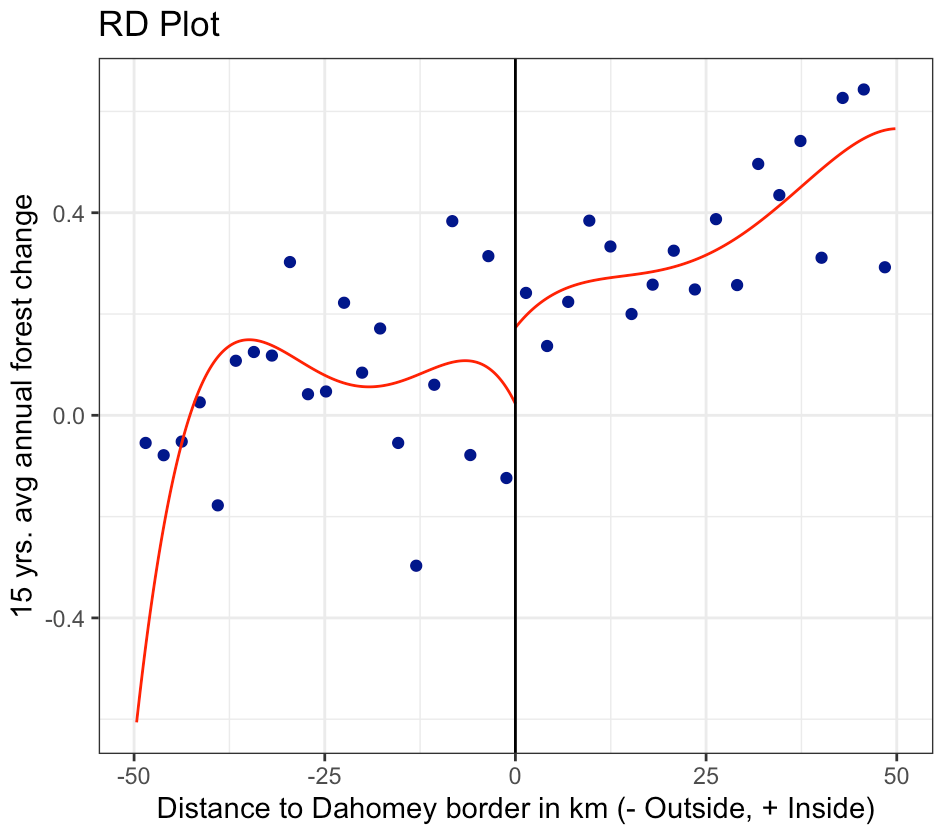
(c) $\Delta\text{Cover}^{15y}_{jb}$

Figure 8: Binned means for 5, 10 and 15 years average annual forest change. The x axis represents distance to the historical boundary of Kingdom of Dahomey. Negative distance = outside Dahomey; positive distance = inside Dahomey. Fourth degree polynomial in distance from the border, weighted using a triangular kernel. Bins were selected by an optimal evenly-spaced method and a bandwidth of 50 km.

It would be prudent to discuss these findings in the context of the larger literature on historical persistence. Even though pre-colonial institutions were abolished by the French, and the entire study region has since been subjected to the same formal institutions, it is possible that our findings could be capturing the impact of pre-colonial centralization (Michalopoulos and Papaioannou, 2013; Gennaioli and Rainer, 2007). According to Coşgel et al. (2019), even states who implemented religious legitimacy through theocracy could indeed have high state capacity. As described earlier, the Kingdom of Dahomey was defined by its religion in every sense, however, we do not claim that the persistence of ATR beliefs is the only mechanism linking the historical Kingdom to contemporary forest change outcome but it does seem a significant and plausible channel. The lack of spatially explicit grid cell level data does not allow me to rule out other possible channels.

However, these concerns can be mildly addressed by looking at the ethnic distribution underlying the region of study. The founders and majority ethnic group of Dahomey were the Fon people and those in neighbouring region were the Yoruba of the Oyo Empire. Following Michalopoulos and Papaioannou (2013) in Table F.7, we present the pre-colonial ethnic characteristics of the two groups that are indicative of centralization. We find that for the widely used indicator of political centralization: Jurisdictional Hierarchy Beyond the Local Community both groups were at level 3 i.e. groups that were part of large states. Additionally the settlement patterns across both groups were identical as well. With respect to degree and type of class differentiation, we find a slight difference as the Yoruba had a complex stratification but overall both groups were high on the scale of being stratified societies.

Table 2: Spatial RDD estimates

	$\Delta\text{Cover}^{5y}_{jb}$	$\Delta\text{Cover}^{10y}_{jb}$	$\Delta\text{Cover}^{15y}_{jb}$
	(1)	(2)	(3)
Linear RD Polynomial:
Dahomeyj	0.278	0.344∗∗∗	0.175∗∗
	(0.261)	(0.116)	(0.084)
Quadratic RD Polynomial:
Dahomeyj	0.137	0.342∗∗	0.190∗∗
	(0.330)	(0.160)	(0.089)
Observations	439	439	439
Segment fixed effects	✓	✓	✓
Clusters	24	24	24

• Unit of analysis is 5.6 kms $\times$ 5.6 kms grid cell. Results use equation (18) and control for log(dist. from coast). All estimations use a bandwidth of 30 kms. ^∗p$<$0.1; ^∗∗p$<$0.05; ^∗∗∗p$<$0.01.

5.3 Spirit of Sustainability

These results raise the intriguing question of why is it that adherence to ATR leads to a positive environmental impact. Proposition 2 equation 12 of the model indicates that the level of beliefs directly influence decision to deforest. This is consistent with the core argument of Weber (1904) which states that the unique feature of religion is its potential influence on beliefs that reinforce particular traits and values i.e. religion is sui generis. We hypothesise that several integral aspects of the ATR worldview such as - the manifestation of spirits and divinities in natural forces and phenomena such as rain, thunder, rivers, trees, mountains, forests etc. and the profound connection to land as a link with ancestors (Mbiti, 1990)- generate a set of attitudes within adherents that reflect the spirit of sustainability. Therefore, the substitutability between resource extraction and belief levels is exhibited through sustainable interaction with the environment. For Benin, where the agricultural sector generates around 50 percent of employment and 25 percent of GDP, but is dominated by subsistence farming dependent on rainfall: this spirit would primarily be reflected in sustainable agricultural practices which help increase or sustain land productivity, thus discouraging land clearing and deforestation.

Similar to the rest of West Africa, Benin is facing rapid demographic growth, increasing exposure to climate change, rising fuelwood production to meet energy demands and lack of incentives for sustainable activities: resulting in land degradation, soil erosion and nutrient depletion leading to the primary driver of deforestation that is extensive shifting agricultural (World Bank, 2020). Between 2005 and 2015, while croplands increased from 3.7 to 5.3 million ha, forests experienced a 22 percent decline. Despite these alarming rates, concomitantly, detailed ecological knowledge about the resources and its impact continues to persist locally amongst farmers and is reflected in several indigenous farming practices (Brouwers, 1993; Saïdou et al., 2004; Gaoue and Ticktin, 2009; Boko, 2017). Some examples are rotating crops and embracing diversity, planting cover crops, no-till systems (or reduced till), integration between livestock and crops, and agroforestry practices (Piñeiro et al., 2020).

However, detailed knowledge of sustainability may not always translate into sustainable practices. Therefore, using a nationally representative household agricultural survey we provide motivating evidence on the usage of sustainable agricultural practices by ATR households in Appendix G. We find that households with ATR heads are indeed more likely to adopt farming practices such as no tillage, use of organic fertilizers and inter-cropping and agro-forestry. Taking reassurance from the positive correlation, we move to a more spatially explicit estimation. If indeed ATR adherents employ sustainable agricultural activities deterring them from practicing extensive shifting agriculture, one should be able to observe its ecological impact in terms of vegetation cover. Utilizing the additional information in the global fractional vegetation cover dataset, we calculate the five year average annual change in short vegetation (SV) and bare ground (BG) for each 10 kms $\times$ 10 kms grid cell as given by (14). Song et al. (2018) define land degradation as the occurrence of short vegetation loss accompanied by bare ground gain ($\Delta\text{SV}\downarrow\;\Delta\text{BG}\uparrow$), and deforestation for agricultural expansion as tree canopy loss accompanied by short vegetation gain ($\Delta\text{TC}\downarrow\;\Delta\text{SV}\uparrow$). Exploiting this information, we create the following binary variables:

$$\textit{Degr}^{5y}_{it}=\begin{cases}1,&\text{if}\ \Delta\text{SV}^{5y}_{it}<0\;\&\;\Delta\text{BG}^{5y}_{it}>0\\ 0,&\text{otherwise}\end{cases}$$

$$\textit{Exp}^{5y}_{it}=\begin{cases}1,&\text{if}\ \Delta\text{Cover}^{5y}_{it}<0\;\&\;\Delta\text{SV}^{5y}_{it}>0\\ 0,&\text{otherwise}\end{cases}$$

$\textit{Degr}^{5y}_{it}$ and $\textit{Exp}^{5y}_{it}$ indicates if the grid cell $i$ at time $t$ sustained deforestation due to land degradation or agricultural expansion in the past five years. Using this as an outcome variable, we estimating regression of the form described in equation (16). Table F.9 presents the results. In columns (1) and (3), we find that a 1 percentage point increase in ATR adherence has no significant effect on the probability of the grid having experienced agriculture related deforestation or land degradation. The insignificance of this correlation is in itself encouraging and consistent with our hypothesis of the role of sustainable environmental interaction. In columns (2) and (4) we create a dummy indicator ATR${}^{q(75)}_{it}$ for grids that fall within the upper quartile of the adherence distribution. We find that being a high adherence ATR cell significantly reduces the probability of deforestation for agricultural purposes by 22%. Therefore, based on these findings, one can infer that the adoption of sustainable practices by ATR adherents is a viable mechanism influencing average annual change in forest cover.

6 Structural Estimates & Spatial Forest Distribution

In this section we fit the model to the FVC and DHS data and estimate its structural parameters. We then show how the equilibrium spatial density predicted by the model fits well the data, and obtain a counterfactual density of the forest cover resulting from a scenario in which ATR adherence is uniformly set to zero. In all that follows we will assume infinitely-lived agents, as having a fully explicit of the problem simplifies identification and estimation considerably.

6.1 Natural forest regeneration rate ($\mu$)

A first issue in identifying the model’s structural parameters is to disentangle the “uncontrolled” drift parameter $\mu$ from the forest consumption $q$ function of all model parameters in equation (2), which characterizes the natural regeneration rate of forest resources. Estimating the drift from individual trajectories in (3), or alternatively from the country-level geometric mean in (19), does not allow one to identify separately $\mu$ from $q^{i}$ or $\int_{A}\bar{q}p_{0}(da)$. Therefore, we search the FVC dataset for an area where $q=0$ in order to capture the natural rate of growth of forests. However, for Benin which is a narrow, key-shaped country, measuring about 325 kms at its widest point and is highly densely populated (see Figure F.6) this seems infeasible. Therefore, as the next best option we use regions where it is plausible to assume that human forest consumption $q^{*}$ is zero. We focus on the W-Arly-Pendjari (WAP) Complex which is a transnational park shared between the Republic of Niger, Burkina Faso and the Republic of Benin and has been a part of the UNESCO World Heritage List since 1996. The park covers a major expanse of intact Sudano-Sahelian savannah, with vegetation types including grasslands, shrub lands, wooded savannah and extensive gallery forests.

We first obtain the forest cover data for areas of WAP falling within Benin corresponding to the W and Pendjari national parks, shown in Figure F.12. We then estimate the parameters based on the construction of a likelihood function derived from the transition probability density of the discretely sampled data. This approach is explained as follows. Suppose $p(X_{it}|X_{it-1},\theta)$ is the transition probability density. The Markov property of equation (2) implies a log-likelihood function for the discrete sample given by $l_{TD}(\Theta)=\log(p(X_{ih}|X_{(i-1)h};\Theta))$. The resulting estimator will be consistent, asymptotically normally distributed and asymptotically efficient under the usual regularity conditions for maximum likelihood estimation in dynamic models (Phillips and Yu, 2009; Hall and Heyde, 2014). To perform exact ML estimation, one needs a closed form expression for $l_{TD}(\Theta)$. It is a well-known result that an uncontrolled geometric Brownian motion, via solving its corresponding Kolmogorov equation, admits a closed form, log-normal transition density:

$$p^{WAP}(x,t+dt|x_{0},t;[\mu,\sigma]) = \frac{1}{x\sigma\sqrt{2\pi dt}}\exp\left(-\frac{1}{2\sigma^{2}dt}\left[\log\left(\frac{x}{x_{0}}\right)-\left(\mu-\frac{\sigma^{2}}{2}\right)t\right]^{2}\right).$$

The discretization of the time grid has to be equivalent to the yearly frequency of the data, and thus we fix $dt=1$. Fitting this function to the data via ML provides me with an estimate of $\mu=0.065$ (95% CI: 0.01,0.12) i.e. a yearly “untouched” growth rate of 6.5% in Benin based on the FVC dataset, which we consider to be a reasonable estimate of the natural growth rate of the forest resources $\hat{\mu}$. Similarly, we estimate $\sigma^{2}$ by an equivalent procedure over the entire forest cover within Benin, since the diffusion coefficient is assumed in the model to be constant across grids. This estimation yields a drift coefficient of $0.016$ (95% CI: 0.012,0.02), corresponding to a growth rate of 1.6% which consistently with our model is less than $\mu$ as the estimate is net of the overall deforestation rate, and strengthens the conjecture of $\mu$ being estimated consistently within the national parks. We also obtain an estimate of $\hat{\sigma}=0.24$, corresponding to a variance of 5%.

6.2 Optimal extraction, beliefs distribution and scarcity

Having identified $\mu$, we can now obtain a measure of the optimal forest consumption policy $q^{*}$ implied by the framework for each grid in the dataset. Given the linearity in $X$ of the optimal policy (22) and the form of each SDE (19), together with a time discretization, imply that $q^{MFE}$ can be recovered as

$$\mathbb{E}(X_{t+dt}-X_{t})=\mathbb{E}X_{t}(\hat{\mu}-\hat{q}^{MFE})dt$$

where the expectation is conditional on the beliefs distribution $p_{0}(a)$. Furthermore, the term $\mathbb{E}(\hat{\mu}-q^{MFE})$ is time-invariant and can be thus obtained from each $\frac{X_{t+1}-X_{t}}{X_{t}}$ across both grids and years. The density estimation of the distribution of grid cells by $\hat{q}^{MFE}/x$ over time is shown in Figure F.13. We now proceed to estimate the beliefs distribution $p_{0}(a)$. Our initial guess of a log-normal distribution fits each year the data quite poorly across grids so we compare a Pareto and a Gamma distribution, which both fit the data well. An AIC criterion leads me to choose (marginally) the Gamma distribution with shape parameter $k_{a}=0.473$ (CI: 0.382, 0.564) and rate $\theta_{a}=0.039$ (CI: 0.027, 0.051). We also estimate shape and rate parameters for each year, and find no significant difference at 95% confidence across the years. The distribution fit via plotting the theoretical and observed distributions as well as a Q-Q plot are shown in Figure F.14.

We now proceed to estimate the parameter which drives the mean-field interactions in the model, $\gamma$, the shape of the function associated with scarcity. We assume $\rho=0.02$ and search the literature for $\eta$. The reason behind assuming $\eta$ instead of estimating lies in the fact that the integral $\int_{A}g^{*}(a)p_{0}(da)$ has no closed form except for extremely specific, almost trivially simplified parametric assumptions for $g$, and always includes $\eta$. This would require techniques such as Monte Carlo integration in order to estimate simultaneously $\eta$ and $\gamma$, and we leave this for future work with more involved parametrizations. We assume $\eta\in[3,5]$ as estimated by Katic and Ellis (2018). The authors calibrate the risk aversion parameters for farming households in Ghana which are primarily characterized by small land holdings of low input–output farming systems. In addition to being in the same region, the households utilized in the study can be considered representative of Benin where the agricultural sector generates over 50 percent of employment, 25 percent of GDP and is dominated by subsistence farming dependent on rainfall.

Equipped with $\eta$, numerical evaluation of the integral $\int_{A}g^{*}(a)p_{0}(da)$, where we assume $g(a)=(1+a)$, is a simple matter. We now estimate $\gamma$ with a standard generalized method of moments procedure over the moment condition induced by the optimal extraction (7). Since the model implies that $q^{MFE}$ is time-invariant and associated to a different level of ATR adherence across grids, this allows me to exploit the entire sample’s variation over ATR beliefs. The moment condition imposes that the optimal $q^{MFE}$ matches the empirical quantity $\hat{q}^{MFE}$ obtained earlier. The estimation is straightforward, uses the Brent method with an optimal weighting matrix and yields an estimate of $\hat{\gamma}=3.12$ (CI: 2.78, 3.46) when $\eta=4$. This estimate ranges between 2.898 (CI: 2.63, 3.16) associated with $\eta=3$ to 3.340 (CI: 2.93, 3.74), which means the estimation is stable with respect to reasonable choices of $\eta$. The boundary case of $\eta=1$ (log utility) yields $\hat{\gamma}=2.20$ (CI: 2.14, 2.25).

Table 3: Model parameter estimates, confidence intervals and methods used

	Parameter	Estimate	95% CI	Method
	(1)	(2)	(3)	(4)
	$\mu$	0.0651	(0.01,0.12)	MLE on TPD (WAP data only)
	$\sigma$	0.2423	(0.149, 0.335)	MLE on TPD
	$k_{a}$	0.405	(0.374, 0.435)	MLE
	$\theta_{a}$	0.041	(0.036, 0.046)	MLE
	$\rho$	0.02
	$\eta$	4	(3, 5)	Estimated by Katic and Ellis (2018)
	$\gamma$	3.158	(2.81174, 3.50466)	GMM

• MLE refers to maximum likelihood estimation. TPD refers to transition probability density. WAP refers to W-Arly-Pendjari complex. GMM refers to generalized method of moments.

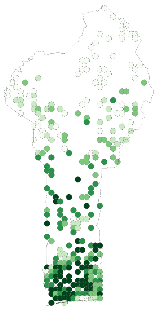
(a) Observed

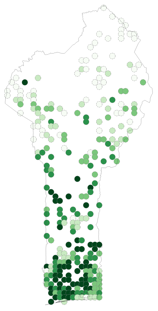
(b) Predicted

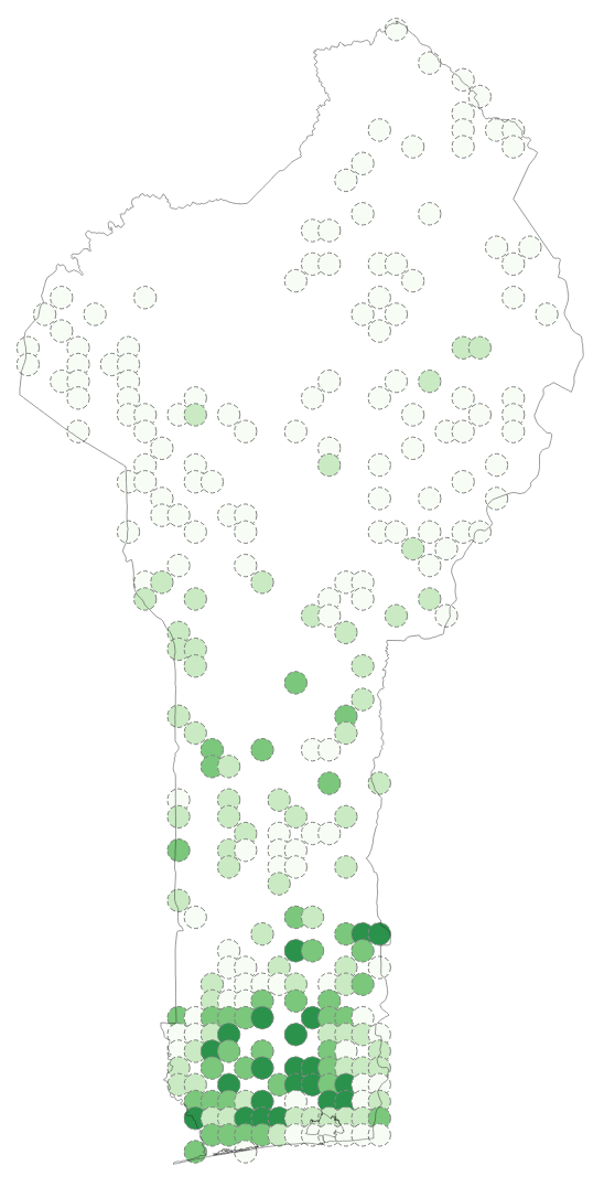
(c) No ATR adherence

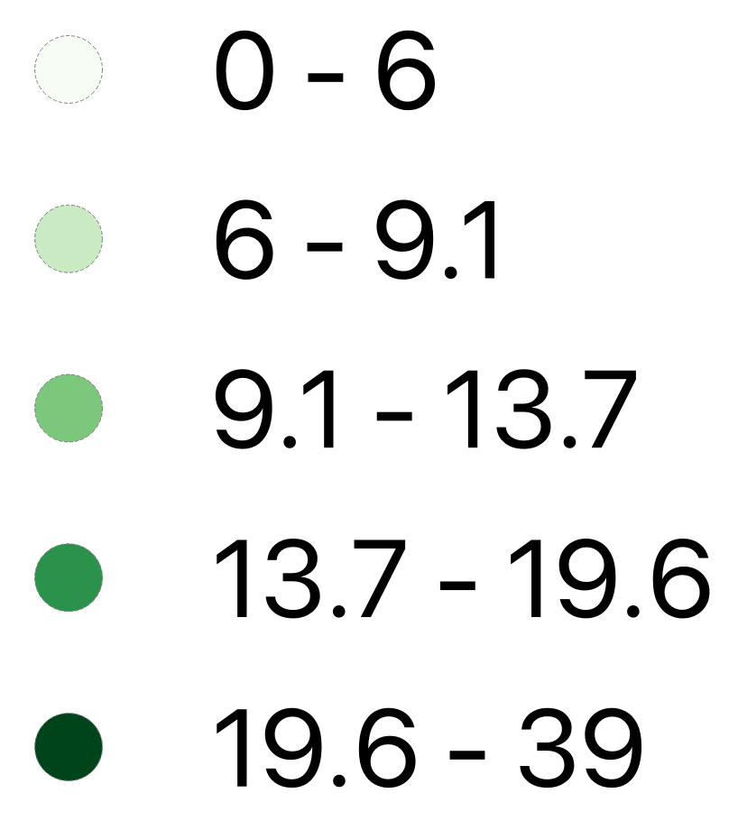
(d)

Figure 9: Observed, predicted and counterfactual spatial forest cover distributions for 2016.

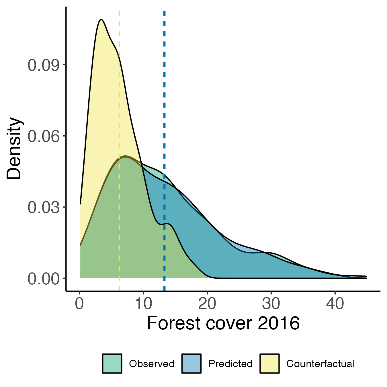
(a)

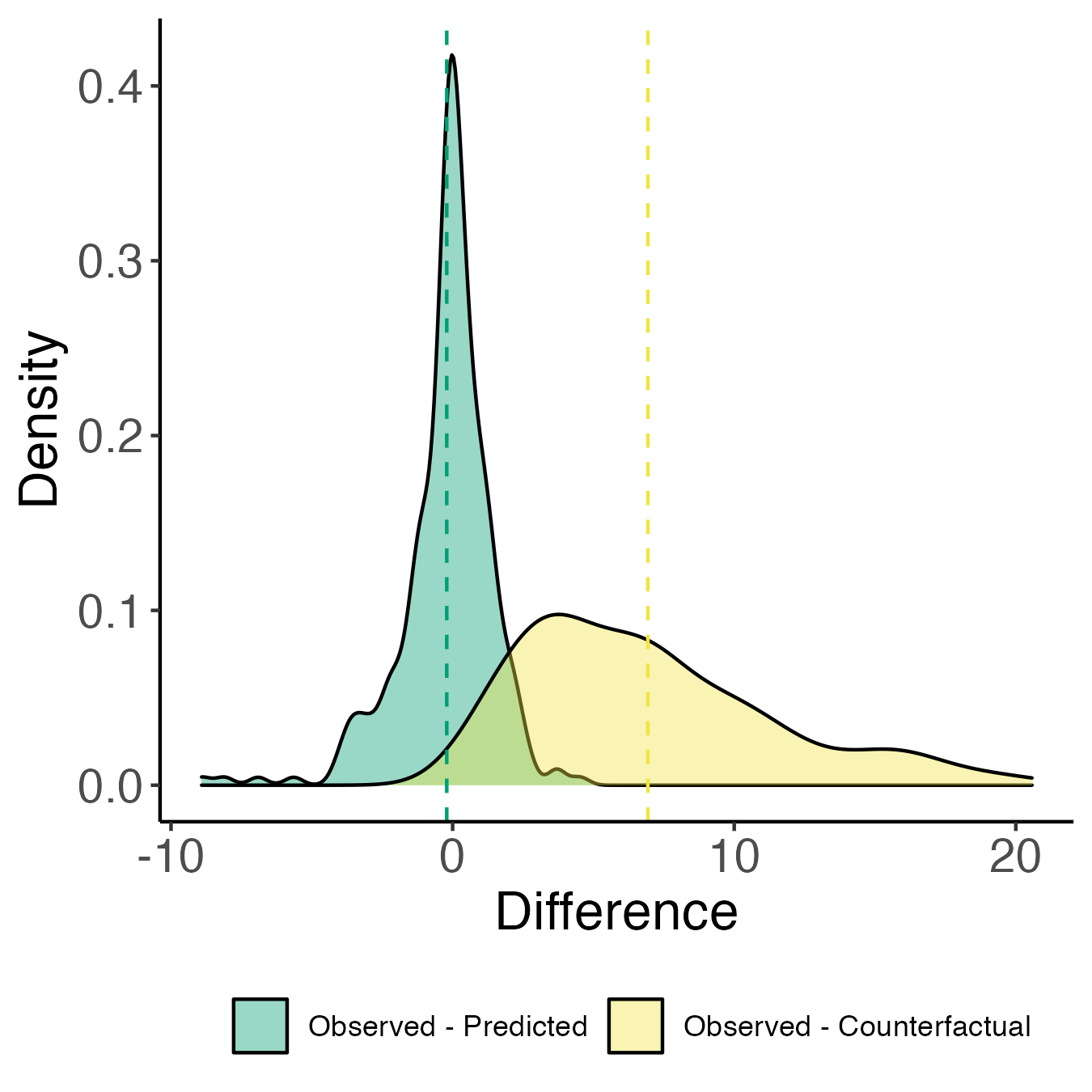
(b)

Figure 10: Density estimation of the distribution of grid cells for 2016 by (a) observed, predicted and counterfactual forest cover and (b) difference between observed and predicted, and observed and counterfactual.

We can now finally show how the equilibrium distribution of the forest cover predicted by the model fits well the observed spatial forest distribution, as well as obtain the counterfactual forest cover distribution resulting from setting all belief levels to zero. The former is obtained using the estimates from Table 3 in the decomposition of (5) and the resulting joint lognormal-Gamma distribution of forest and beliefs evaluated at the estimated model parameters. The estimated expected grid-level forest cover for 2016 is then obtained via the closed-form solution of the SDE associated with (3). The counterfactual distribution is obtained by setting $a=0$ in $q^{MFE}$, which essentially removes all heterogeneity in beliefs and yields an initial condition $p_{0}(dx,da)=p_{0}(dx,\delta(a=0))$, where $\delta(a)$ is the Dirac delta function, only dependent on initial forest endowments. The expected counterfactual forest cover is obtained equivalently using the SDE solution, which we note corresponds to an equilibrium extraction $q^{MFE}=\tilde{\rho}\left(\frac{\gamma-1}{\gamma}\right)X$. Figure 9 plots the on the left panel the observed spatial forest distribution, on the middle panel the distribution implied by the model at the estimated parameters and on the right panel the counterfactual one. The left panel of Figure 10 plots the same density estimates showing how the observed and predicted forest cover distribution match closely, and how the counterfactual distribution that imposes everyone to have no ATR adherence is clearly first-order dominated by the other two. The right panel of Figure 10 further clarifies this point, showing the residual density of the difference between observed and predicted forest cover to be centered on zero (mean: -0.208, median: 0, std. dev: 1.632) and the residual density of the difference between observed and counterfactual to be firmly defined on the positive domain (min: 0.131, max: 20.57). Furthermore, the average difference between observed and counterfactual forest cover is of 6.9%, ranging from a minimum of 0.1% to a maximum of 20% forest loss consequent to removing uniformly all ATR adherence within Benin. Figure F.15 shows the good fit of the spatial (marginal) forest cover with the lognormal spatial density predicted by the model, evaluated at the estimated parameters, by plotting the empirical histogram against the theoretical density (left panel), as well as a Q-Q plot between the two (right panel). Lastly, Figure F.16 presents the predicted (left) and observed (right) joint spatial densities of both ATR and forest cover.

7 Conclusion

Can religious beliefs have an effect on environmental outcomes? We answer this question by studying ATR, in whose cosmology forests are sacred. We build a continuous time non-market interaction model of a continuum of agents with heterogeneous religious adherence and study its effect on the spatial density of forest cover. The mean field equilibrium extraction policy highlights the full coupling of the joint dynamics of both individual beliefs and their distribution in the population, which is central to explaining the impact ATR adherence has on forest use. The model predicts that for any given belief distribution in the population, a higher individual ATR adherence implies a decline in the extraction of forest resources. Conversely, we find that an increase in the population average adherence implies an increase in the localized forest extraction.

We test empirically the model predictions using micro data from Benin, a country that has experienced a renaissance in ATR and where its adherence is freely reported. Using an instrumental variable strategy that exploits the variation in proximity to the Benin- Nigeria border, and a spatial regression discontinuity design, we provide evidence that the ATR-forest link is indeed positive, causal and robust. Finally, we estimate the model parameters and show that the equilibrium spatial density predicted by the model fits well the data, and obtain a counterfactual density of the forest cover resulting from a scenario in which ATR adherence is uniformly set to zero. This paper, therefore, constitutes to our knowledge the first systematic empirical and theoretical evidence on the effect of religious beliefs on environmental outcomes.

Appendix A Model solution and proof of existence of a mean-field equilibrium for finitely-lived agents

Let us first show the reason behind the particular form of coupling given by (6): one can explicitly show the dynamics of the (geometric) average forest cover. Since all agents face idiosyncratic and independent Brownian motions, a straightforward application of Itô’s lemma yields

$$d\log{X_{t}}=\left(\mu-\frac{\sigma^{2}}{2}-\bar{q}_{t}\right)dt+\sigma dW_{t}$$

where we conjecture the mean policies to be linear in $X$, and thus assume $\bar{q}_{t}\in[0,1]$ to be the average fraction of forest consumed by the population at each $t$. The dynamics of the average forest cover $\bar{X}_{t}$ are given therefore by

$$d\bar{X}_{t}:=de^{\mathbb{E}[\log{X_{t}}|\mathcal{F}_{t}^{a}]} = \bar{X}_{t}\left(\mu-\frac{\sigma^{2}}{2}-\int_{A}\bar{q}_{t}p(da)\right)dt.$$ (19)

$$= \bar{X}_{t}\bar{\mu}^{a}dt.$$

The drift $\bar{\mu}^{a}$ represents how the average dynamics depend not only on the ecological parameters $\mu$ and $\sigma$, but also on the heterogeneity in beliefs within the population.

For simplicity we now choose a bequest function of shape $b(x_{T},T)=B\frac{x^{1-\eta}\bar{x}^{1-\gamma}}{(1-\eta)(1-\gamma)}$, where $B=b^{\frac{1}{\eta}}$, meaning that at $T$ each individual will leave a fraction $b$ of the terminal resources. The HJB equation in the extended state space $(x,\bar{x},t)\in\mathbb{R}^{+}\times\mathbb{R}^{+}\times[0,T]$ becomes

$$-V_{t}+\rho V=\sup_{q}\left[\frac{(q\ g(a))^{1-\eta}}{1-\eta}\frac{\bar{x}^{1-\gamma}}{1-\gamma}-qV_{x}\right]+\mu xV_{x}+\frac{\sigma^{2}}{2}x^{2}V_{xx}-\bar{\mu}^{a}\bar{x}V_{\bar{x}}.$$ (20)

with boundary condition $V(x,\bar{x},T)=b(T)^{\eta}$. The supremum is obtained with the optimal policy

$$q^{*}(X_{t},\bar{X}_{t},a,t)=\left(\frac{\bar{X}_{t}^{1-\gamma}}{(1-\gamma)V_{x}}\right)^{1/\eta}g(a)^{-\frac{\eta-1}{\eta}}.$$ (21)

Inserting (21) in the HJB yields the nonlinear PDE

$$-V_{t}+\rho V = \frac{\bar{x}^{1-\gamma}}{(1-\eta)(1-\gamma)}\left[\frac{(1-\gamma)V_{x}}{\bar{x}^{1-\gamma}}\right]^{\frac{\eta-1}{\eta}}-\left[\frac{(1-\gamma)V_{x}}{\bar{x}^{1-\gamma}}\right]^{-1/\eta}\tilde{g}(a)V_{x}$$

$$+\mu xV_{x}+\bar{\mu}^{a}\bar{x}V_{\bar{x}}+\frac{\sigma^{2}}{2}x^{2}V_{xx}.$$

Using as ansatz for the value function a time-separable guess $V(x,\bar{x},t)=f(t)^{\eta}\frac{x^{1-\eta}\bar{x}^{1-\gamma}}{(1-\eta)(1-\gamma)}$ that exploits the homothetic and multiplicative form of the objective function, we obtain the optimal individual extraction

$$q^{*}(X_{t},a,t)=\frac{g(a)^{-\frac{\eta-1}{\eta}}}{f(a,t)}X_{t}$$ (22)

where

$$f(a,t) = \exp\left(\tilde{\rho}(T-t)-\frac{1-\gamma}{\eta}\int^{T}_{t}\int_{A}\bar{q}_{s}p(da)ds\right)B+$$

$$+\frac{1+(\eta-1)g(a)^{-\frac{\eta-1}{\eta}}}{\eta}\exp\left(-\tilde{\rho}t+\frac{1-\gamma}{\eta}\int_{0}^{t}\int_{A}\bar{q}_{s}p(da)ds\right)\times$$

$$\times\int_{t}^{T}\exp\left(\tilde{\rho}s-\frac{1-\gamma}{\eta}\int_{0}^{s}\int_{A}\bar{q}_{r}p(da)dr\right)ds,$$

$$\tilde{\rho} = \frac{1}{\eta}\left[\mu(2-\eta-\gamma)-\frac{\sigma^{2}}{2}(\eta(1-\eta)+1-\gamma)-\rho\right].$$

The term $1/f(a,t)$, which is obtained using the boundary condition on $V(x,\bar{x},T)$, depends clearly on the bequest $B$ and continuously on a combination of all model parameters as well as the mean extraction integrated over the whole beliefs distribution. Note that for $a=0$ and $p(a)=0$ one reverts to a standard consumption problem under uncertainty. Note that this result validates our conjecture of the (geometric) average extraction policy within the population being linear in $x$.

What is now required is to prove the existence of a mean-field equilibrium. Let $q^{*}_{t}$ be an admissible and $\mathcal{F}^{a}_{t}$-measurable extraction policy for our problem, and let $\bar{X_{t}}$ be a $\mathcal{F}^{a}_{t}$-measurable random variable given by $\bar{X_{t}}=\exp(\mathbb{E}\log X^{*}_{t})$, where $X^{*}_{t}$ is the forest cover associated with the policy $q^{*}_{t}$. The policy $q^{*}_{t}$ is a mean-field equilibrium if $q^{*}_{t}$ is optimal for each agent upon this choice of $\bar{X_{t}}$, under the consistency condition that $\bar{X}_{t}=\exp\int\log x^{*}p(dx^{*},da,t)$ for all $t\in[0,T]$. This implies that the equilibrium is associated with a continuum of optimal choices, weighed by each individual adherence, in a framework where essentially each agent in the continuum faces an independently distributed copy of the same optimization problem, based on the intial draw from the beliefs distribution. In other words, the equilibrium happens at the point for which $\int_{A}q^{*}/x\ p_{0}(da)=\int_{A}\bar{q}p_{0}(da)$ for all $t\in[0,T]$.

This is the case if there exists a function for the population forest consumption averaged over the whole beliefs distribution $\bar{q}^{a}_{t}:[0,T]\to[0,1]$ that solves the fixed point relation given by

$$\int_{A}\bar{q}_{t}p_{0}(da):=q^{a}_{t}=\int_{A}\frac{g(a)^{-\frac{\eta-1}{\eta}}}{f(a,t)}p_{0}(da).$$ (24)

There exists an equilibrium where each individual consumes an amount of forest inversely proportional to her own individual beliefs $a$ and to the collective average actions $q^{a}_{t}$ of the population, which are defined by the fixed point in (24). This equilibrium exists if $\gamma\geq 1$ and if $\eta\geq 1$, which is already a requirement in our framework, and thus it always exists within the model’s parametric space. The proof reads as follows:

Proof. Assuming the right-hand side exists and is bounded, which is equivalent to assuming a reasonably well-behaving distribution of beliefs $p(a)$, we study the map $Q_{A}:Q[(0,T)]\to Q([0,T)]$ given by

$$Q_{A}(q^{a})_{t}:=\int_{A}\frac{1}{f(a,q^{a},t)(1+a)}p_{0}(da)$$

This map is a contraction if $\eta$ is not too small and $\gamma\geq 1$, since it is defined in $[0,T]\to[0,1]$ and for any $q_{1}^{a},q_{2}^{a}\in Q^{A}[(0,T)]$ in which $q_{i}^{a}=\int_{A}q_{i}p(da)$ (i.e. the dependence on $a$ has been integrated out) one has

$$|Q_{A}(q_{1}^{a})_{t}-Q_{A}(q_{2}^{a})_{t}| = \sup_{t\in[0,T]}\left|\int_{A}\frac{1}{f(a,q^{a}_{1},t)(1+a)}p_{0}(da)-\int_{A}\frac{1}{f(a,q^{a}_{2},t)(1+a)}p_{0}(da)\right|$$

$$= \sup_{t\in[0,T]}\left|\int_{A}\frac{f(a,q^{a}_{1},t)-f(a,q^{a}_{2},t)}{f(a,q^{a}_{1},t)f(a,q^{a}_{2},t)}\frac{1}{1+a}p_{0}(da)\right|$$

$$\leq \int_{A}\frac{\eta e^{\tilde{\rho}T+\frac{1-\gamma}{\eta}\int_{0}^{t}|q_{1}^{a}-q_{2}^{a}|ds}}{(1+a)Be^{\tilde{\rho}T-\frac{1-\gamma}{\eta}\int_{0}^{t}|q_{1}^{a}-q_{2}^{a}|ds}+(\eta+a)\int_{t}^{T}e^{\tilde{\rho}s-\frac{1-\gamma}{\eta}\int_{0}^{s}|q_{1}^{a}-q_{2}^{a}|dr}ds}p_{0}(da)$$

$$\leq C\ ||q_{1}^{a}-q_{2}^{a}||,$$

for some constant $C$ in which $a$ has been integrated out, as $\tilde{\rho}$ is bounded as long as $\eta$ doesn’t go to zero. One then can apply Banach’s fixed point theorem which guarantees the existence of a solution. Note that this “minimum” $\eta^{0}\in(0,1]$, as for $\eta=1$ (log utility of forest consumption) we have $f(a,t)\to f(t)$ and the previous expression can be written as

$$|Q_{A}(q_{1}^{a})_{t}-Q_{A}(q_{2}^{a})_{t}| \leq f(t)^{-1}\int_{A}\frac{1}{1+a}p_{0}(da)$$

$$\leq \frac{e^{\tilde{\rho}t+(1-\gamma)\int_{0}^{t}|q_{1}^{a}-q_{2}^{a}|ds}}{Be^{\tilde{\rho}T-(1-\gamma)\int_{0}^{t}|q_{1}^{a}-q_{2}^{a}|ds}+\int_{0}^{T}e^{\tilde{\rho}s-(1-\gamma)\int_{0}^{s}|q_{1}^{a}-q_{2}^{a}|dr}ds}\int_{A}\frac{1}{1+a}p_{0}(da)$$

which is clearly holding, since $Q_{a}(q)_{t}=f(t)^{-1}\int_{A}\frac{1}{1+a}p_{0}(da)$, as long as $\gamma\geq 1$.

End of proof

We can finally expose the drivers of the joint individual and mean decisions: individual adherence $a$ reduces each individual’s forest use decisions via the direct effect seen in (22). However, the distribution of ATR beliefs within the population, defined by $p_{0}(a)$, affects the individual policy via $\int_{A}\bar{q}_{t}p_{0}(da)$, the mean of the forest consumption policies averaged over all beliefs. To see this, first focus on the end-of-life case where $t=T$. Here, all that matters to the individual is the bequest $B$, as it’s immediately seen from (A) that $f(a,T)=B$. The mean extraction policy in the population is then

$$\int_{A}\bar{q}_{T}p_{0}(da)=\frac{1}{B}\int_{A}g(a)^{-\frac{\eta-1}{\eta}}p_{0}(da)$$

which is easily seen to be decreasing in the first moment of $p_{0}(da)$ (notice that $\tilde{g}\to 0$ for $a\to\infty$) for all reasonably well-behaving beliefs distributions.

Once the average forest consumption $\bar{q}_{t}$ is obtained from (22) and inserted in $\bar{f}(a,t):=f(a,t)|_{q=\bar{q}}$ from (24) to yield $q^{*}(X_{t},a,t)$, one can integrate in time the equilibrium Kolmogorov equation to obtain the (transition) spatial density for $p_{0}$-almost any $a$, as given by

$$p^{a}(x,t|p_{0}(x_{0}),0)=\frac{1}{x\sigma\sqrt{2\pi t}}\exp\left(-\frac{1}{2\sigma^{2}t}\left[\log\left(\frac{x}{x_{0}}\right)-\left(\mu-\frac{\sigma^{2}}{2}\right)t+\int_{0}^{t}\frac{g(a)^{-\frac{\eta-1}{\eta}}}{\bar{f}(a,t)}ds\right]^{2}\right).$$ (25)

We now report a fully-solved restrictive yet illustrative example for log-utilities where $\eta=\gamma=1$, which is the limit case where the problem is decoupled and the mean field is collapsed to individual agents. Note that log utility implies $u_{qa}=0$, meaning there is no substitutability in the utility drawn between forest consumption and scarcity. The example shows how a country with a low average adherence to traditional beliefs will have a decreased average forest cover, even though local communities (at a grid level, for example) can exhibit higher forest cover due to the effect of their local higher levels of adherence.

In the log-utility case the problem is effectively decoupled and one can obtain the full form of the average forest cover distribution. It is easily shown in this case that

$$\int_{A}\bar{q}_{t}p_{0}(da)=e^{-\tilde{\rho}(T-t)}\frac{\tilde{\rho}}{1+\tilde{\rho}B}\int_{A}\tilde{g}(a)p_{0}(da),$$

which allows me to use the Kolmogorov equation given by the second line of (4) and show that the equilibrium forest cover averaged over all individual beliefs behaves according to the transition density

$$p(x^{a},t) = \frac{1}{x^{a}\sigma\sqrt{2\pi t}}\exp\left(-\frac{1}{2\sigma^{2}t}\left[\log\left(\frac{x^{a}}{x^{a}_{0}}\right)-\left(\mu-\frac{\sigma^{2}}{2}\right)t+\right.\right.$$

$$\left.\left.+\frac{\tilde{\rho}}{1+\tilde{\rho}B}\int_{A}\int_{0}^{t}e^{-\tilde{\rho}(T-s)}\tilde{g}(a)p_{0}(da)ds\right]^{2}\right).$$

The average forest cover in the population is therefore decreasing in the expectation of $1/(1+a)$ with respect to the beliefs measure. As a simple example, assume $\tilde{g}(a)=(1+a)^{-1}$ (which implies assuming $g(a)=(1+a)^{\eta/(\eta-1)}$) and that the beliefs are uniformly distributed among the population with cumulative density $p(a)=a/\bar{a}$ defined between $0$ (where the problem collapses to a deterministic one) and a maximum adherence $\bar{a}$. Then it’s a simple exercise to show that the integral of $1/(1+a)$ over the measure $p_{0}(da)$ is

$$\int_{A}\frac{1}{1+a}p_{0}(da)=\frac{\log(\bar{a}(1+\bar{a})-\log(\bar{a})}{\bar{a}}$$

which is decreasing in both the maximum $\bar{a}$ and thus the average adherence $\bar{a}/2$. This implies that a country with a low average adherence to traditional beliefs will have a decreased average forest cover, even though local communities (at a grid level, for example) can exhibit higher forest cover due to the effect of their local higher levels of adherence. This phenomenon is what we observe in the data.

Appendix B Proof of Proposition 1

Using as ansatz $V(x,\bar{x})=A\frac{x^{1-\eta}\bar{x}^{1-\gamma}}{(1-\eta)(1-\gamma)}$ we obtain that the constant $A$ (conditional on the realization of $a$) as given by

$$A = \left(\frac{C}{1+(\eta-1)g(a)^{-\frac{\eta-1}{\eta}}}\right)^{-\eta},$$

$$\tilde{\rho} = \mu(\eta+\gamma-2)-\frac{\sigma^{2}}{2}(\eta(\eta-1)+\gamma-1)+\rho,$$

$$C = \tilde{\rho}-(\gamma-1)\int_{A}\bar{q}p_{0}(da),$$

which in turn yields an optimal individual forest extraction given by

$$q^{*}(X_{t},a) = g^{*}(a)\ C\ X_{t}.$$ (26)

$$g^{*}(a) = \frac{g(a)^{-\frac{\eta-1}{\eta}}}{1+(\eta-1)g(a)^{-\frac{\eta-1}{\eta}}}.$$

This expression makes the fixed point problem solved in the finite-time case substantially easier to deal with: again, an equilibrium exists if the (now constant) $\bar{q}=\int_{A}q^{*}/xp_{0}(da)$ implying that the mean extraction policy averaged over the belief distribution is

$$\int_{A}\bar{q}p_{0}(da)=\frac{\tilde{\rho}\int_{A}g^{*}(a)p_{0}(da)}{1+(\gamma-1)\int_{A}g^{*}(a)p_{0}(da)}\leq\tilde{\rho}.$$ (27)

Since this quantity needs to be positive, we will restrict as in the finite-time cases to the situation in which $\gamma\geq 1$. Equation (27) identifies an admissible mean-field equilibrium for some values of $\gamma$ between 0 and 1, but it would require bounding the expectation of $1/a$ and thus we prefer to focus on the $\gamma\geq 1$ case and leave the beliefs distribution unrestricted. The full mean-field equilibrium associated with (27) is

$$q^{MFE}(X_{t},a)=\tilde{\rho}\ g^{*}(a)\left(1-\frac{\int_{A}g^{*}(\bar{a})p_{0}(d\bar{a})}{1+(\gamma-1)\int_{A}g^{*}(\bar{a})p_{0}(d\bar{a})}\right)X_{t},$$ (28)

where we write $p_{0}(d\bar{a})$ to distinguish the individual adherence $a$: single realization drawn from the distribution $p_{0}$, from the quantity $\int_{A}g^{*}(\bar{a})p_{0}(d\bar{a})$, which is calculated over all possible realizations of $a$.

We can now use the linearity in $x$ of (28) and the decomposition (5) to obtain the measure in $x$ $p_{0}$-almost any $a$. Using the Kolmogorov equation (4) at the optimal control $q^{MFE}$ for the joint distribution $p(x,a,t)$ we obtain

$$\partial_{t}p(x,a,t)=-\partial_{x}\left[\mu-\tilde{\rho}\ g^{*}(a)\left(1-\frac{\int_{A}g^{*}(\bar{a})p_{0}(d\bar{a})}{1+(\gamma-1)\int_{A}g^{*}(\bar{a})p_{0}(d\bar{a})}\right)\right]x\ p(x,a,t)+\frac{\sigma^{2}}{2}\partial_{xx}x^{2}p(x,a,t).$$

Using (5) and the time invariance of $p_{0}$ one obtains

$$p_{0}(a)\partial_{t}p^{a}(x,t) = -p_{0}(a)\partial_{x}\left[\mu-\tilde{\rho}\ g^{*}(a)\left(1-\frac{\int_{A}g^{*}(a)p_{0}(da)}{1+(\gamma-1)\int_{A}g^{*}(a)p_{0}(da)}\right)\right]x\ p^{a}(x,t)+$$

$$+\frac{\sigma^{2}}{2}p_{0}(a)\partial_{xx}x^{2}p^{a}(x,t),$$

which reduces to

$$\partial_{t}p^{a}(x,t)=-\partial_{x}\left[\mu-\tilde{\rho}\ \int_{A}g^{*}(a)p_{0}(da)\left(1-\frac{\int_{A}g^{*}(a)p_{0}(da)}{1+(\gamma-1)\int_{A}g^{*}(a)p_{0}(da)}\right)\right]x\ p^{a}(x,t)+\frac{\sigma^{2}}{2}\partial_{xx}x^{2}p^{a}(x,t).$$

The reader can now verify the well-known result that the above PDE under the normalization condition $\int p^{a}(dx,t)=1$ for any $a$ is the log-normal transition density shown in Proposition 1.

Appendix C Proof of Proposition 2

The first part of the Proposition is a simple exercise to obtain, as $(d/da)q^{MFE}/x$ maps one-to-one with $g^{*^{\prime}}$. Computing the derivative one obtains

$$g^{*^{\prime}}(a)=-\frac{(\eta-1)}{\eta}\frac{g(a)^{1/\eta}g^{\prime}(a)}{(g(a)+(\eta-1)g(a)^{1/\eta})^{2}}.$$

Since $g^{\prime}(a)\geq 0$ by construction, the result immediately follows. The proof of the second part is slightly more involved. Firstly, since $p_{0}(a)$ is a probability measure it is Lebesgue-integrable and so is its cumulative density $P_{0}(a)$. Parametrizing both as $p_{0}(a;\mu_{a})$ and $P_{0}(a;\mu_{a})$ and assuming that $\partial_{\mu_{a}}p_{0},\partial_{\mu_{a}}P_{0}$ exist and are bounded (a simple requirement that holds for most non-degenerate parametrized distributions), since $g(a)$ is continuous (and thus so is $g^{*}$) one can apply the bounded convergence theorem and show that

$$\frac{d}{d\mu_{a}}\int_{A}g^{*}(a)p_{0}(da;\mu_{a})=\int_{A}g^{*}(a)\partial_{\mu_{a}}p_{0}(da;\mu_{a}).$$

With this result, it is then a simple exercise to show that

$$\frac{d}{d\mu_{a}}\left(\frac{q^{MFE}}{X_{t}}\right)=-\frac{\int_{A}g^{*}(\bar{a})\partial_{\mu_{a}}p_{0}(d\bar{a};\mu_{a})}{\left(1+(\gamma-1)\int_{A}g^{*}(\bar{a})p_{0}(d\bar{a};\mu_{a})\right)^{2}}\tilde{\rho}\ g^{*}(a).$$ (29)

The sign of this derivative is thus determined by the numerator. Integrating by parts and using Fubini’s theorem we obtain

$$\int_{A}g^{*}(\bar{a})\partial_{\mu_{a}}p_{0}(d\bar{a};\mu_{a})=g^{*}(a)\partial_{\mu_{a}}P_{0}(a;\mu_{a})|^{\bar{A}}_{0}-\int_{A}g^{*^{\prime}}(a)\partial_{\mu_{a}}P_{0}(da;\mu_{a}),$$ (30)

where $\bar{A}$ is the upper boundary of the domain of the beliefs distribution. One must now distinguish two cases based on the shape of the domain $A$. Let me begin with the case for which $A$ is unbounded from above, i.e. $A=\mathbb{R}^{+}$. This case includes all distributions with exponential tails such as the log-normal and Gamma families. Using L’Hopital’s rule, since $\gamma\geq 0$ and $\eta\geq 1$ it is a simple exercise to show that

$$\lim_{a\to\infty}\frac{g(a)^{-\frac{\eta-1}{\eta}}}{1+(\eta-1)g(a)^{-\frac{\eta-1}{\eta}}}=0,$$ (31)

which allows to write

$$\int_{0}^{\infty}g^{*}(\bar{a})\partial_{\mu_{a}}p_{0}(d\bar{a};\mu_{a})=-\int_{0}^{\infty}g^{*^{\prime}}(a)\partial_{\mu_{a}}P_{0}(da;\mu_{a}).$$

Since we have assumed $g^{\prime}(a)>0$, one can immediately see that $g^{*^{\prime}}(a)<0$. By the definition (11) of first-order stochastic dominance, an increase in the parameter that ranks the beliefs distributions in such order must generate a shift to the right of the beliefs CDF, hence $\partial_{\mu_{a}}P_{0}(da)\leq 0$. It immediately follows that $\int_{A}g^{*}(\bar{a})\partial_{\mu_{a}}p_{0}(d\bar{a};\mu_{a})<0$ and thus $\frac{d}{d\mu_{a}}q^{MFE}>0$. For the bounded domain case, which applies for example such as the uniform and Beta distributions, one cannot use anymore the fact that $q^{*}(\bar{A})=0$, and one has

$$\int_{A}g^{*}(\bar{a})\partial_{\mu_{a}}p_{0}(d\bar{a};\mu_{a})=q^{*}(\bar{A})\partial_{\mu_{a}}P_{0}(\bar{A};\mu_{a})-\int_{A}g^{*^{\prime}}(a)\partial_{\mu_{a}}P_{0}(da;\mu_{a}).$$

By the definition of $g^{*}$, $g^{*}(\bar{A})\geq 0$. However, as shown before $\partial_{\mu_{a}}P_{0}(da)\leq 0$ and hence the first term on the right-hand side of the previous expression is zero at the maximum. The second term remains negative as shown in the unbounded case, and hence for a general domain $A$ we have $\frac{d}{d\mu_{a}}q^{MFE}>0$. The second result in (3.1) follows immediately from (31), as in (29) $a$ is integrated out and thus only enters $\frac{d}{d\mu_{a}}q^{MFE}$ via $g^{*}(a)$. The proof is thus complete.

Appendix D Risk aversion & Religion

We study the effects of risk aversion on optimal consumption policy in equation (7) as it has been identified as an important mechanism underlying the effects of culture on economic outcomes. We find that while $q^{MFE}_{\eta}<0$, whether $q^{MFE}_{\eta a}<0$ or $q^{MFE}_{\eta a}>0$ depends on if and how one decides to model the relation between risk aversion and religious beliefs in $g(a)$. Prior research focused on Christianity has suggested a positive relationship between risk aversion and religion (Miller and Hoffmann, 1995; Liu, 2010; Dohmen et al., 2011). Consistent with these studies one could model $g(a)=(1+a)^{\frac{\eta-1}{\eta}},\;g_{\eta}>0$. Figure D (a) illustrates this choice and finds that the slope of how forest consumption is changing in risk aversion is increasing in ATR adherence i.e. $q^{MFE}_{\eta a}>0$

Hilary and Hui (2009) and Noussair et al. (2013) both show that the links between risk aversion and religion are related to the social aspects of activities associated with religious practice. They find robust evidence that this positive relationship is principally derived from the social and institutional aspects of church membership. To model the risk aversion - religion link for ATR it is important to reconcile with its distinctive features. As opposed to Abrahamic faiths, ATR is characterized by decentralized and non congregational structure complemented by the lack of emphasis on collective temple/church observance. Therefore in line with studies such as Liu (2010) and Miller (2000) which show no significant relation between risk aversion and religion for Asian traditional religions, which share similar social characteristics to ATR , we could model simply $g(a)=(1+a)$. This choice is illustrated in Figure D (b) which is qualitatively similar to Figure D (a). An alternative choice is to model $g(a)=(1+a)^{\frac{\eta}{\eta-1}},\;g_{\eta}<0$ shown in Figure D (c), In this case one can infer that the effect of risk aversion on forest consumption is decreasing in ATR adherence i.e. $q^{MFE}_{\eta a}<0$.

figure0pt

$g(a)=(1+a)^{\frac{\eta-1}{\eta}}$

0pt

$g(a)=(1+a)$

0pt

$g(a)=(1+a)^{\frac{\eta}{\eta-1}}$

Effect of risk aversion on optimal consumption policy for different levels of ATR adherence $a=1,3,10$. Model parameters: $\gamma=2.5,\mu=0.1,\sigma=0.05,\rho=0.02$. Beliefs distribution: $\exp N(2,0.5)$.

Appendix E Data sources and variable definitions

E.1 Climatic Variables

Climatic variables were obtained from TerraClimate: a dataset of monthly climate and climatic water balance for global terrestrial surfaces from 1958 - 2019. These are available at https://www.climatologylab.org/terraclimate.html and all data have monthly temporal resolution and a 4 km (1/24 degree) spatial resolution. The data cover the period from 1958-2020. The climatic variables used are: precipitation (units = millimeters), temperature (units = Celsius) and Palmer Severity Drought Index (units = unitless). The Palmer Drought Severity Index (PDSI) uses temperature and precipitation data to estimate the relative dryness of a region. Its scale ranges from -10 (very dry) to +10 (very wet) with 0 being normal. A value for moderate drought is -2 while conditions of extreme drought start at -4. The PDSI is best used to quantify long-term drought that has affected a region for several months. These indicators are calculated as the monthly mean for each grid cell and then averaged over twelve months to obtain the yearly variables.

E.2 Geographic Variables

• Elevation and Slope: The terrain data is available at Global Agro-Ecological Zoning (GAEZ) version 4 data portal (https://gaez.fao.org/pages/data-viewer) and comprises of 30 arc second (approximately 1 km at the equator) layers of median altitude (metres) and median terrain slope class. This data has been derived from digital elevation data of the Shuttle Radar Topography Mission (SRTM). The elevation and slope variable used measures the mean elevation and slope class for each grid cell.

• Soil suitability: The data has been obtained from GAEZ, where suitability ratings are assigned based on soil qualities influencing crop performance (nutrient availability, nutrient retention capacity, rooting conditions, oxygen availability to roots, presence of salinity and sodicity, presence of lime and gypsum, and workability) at high, intermediate and low level inputs, by water supply system. We focus on Soil suitability, rain-fed, low inputs typical for subsistence farming and traditional management systems. The data is at the spatial resolution of 5 arc-minute grid cell (which is approximately equivalent to 9.26 km × 9.26 km at the equator).

• Distance to roads: The Benin Road Network shapefile was obtained from the OpenStreetMap data made by World Food Programme (WFP) following the UN Spatial Data Infrastructure - Transportation standards (https://geonode.wfp.org/layers/geonode:ben_trs_roads_osm). For the distance we calculate the straight-line Euclidean distance (in kms) from the centroid of each grid cell to the closest primary and secondary roads.

• Distance to protected areas: The Benin protected areas and forest reserves shapefile was obtained from The Landscapes Portal (http://landscapesportal.org/layers/geonode:protected_areas_ads). For the distance we calculate the straight-line Euclidean distance (in kms) from the centroid of each grid cell to the closest protected area or reserve.

• Distance to waterways: Using the shapefile available at https://data.humdata.org/dataset/hotosm_ben_waterways we calculate the straight-line Euclidean distance (in kms) from the centroid of each grid cell to the closest waterway.

• Distance to coast: We calculate the euclidean distance (in kms) from the centroid of each grid cell to the ocean.

• Distance to Nigerian border: We calculate the straight-line Euclidean distance (in kms) from the centroid of each grid cell to the Nigerian border.

• Latitude and Longitude: We utilise the coordinates of the centroid of each grid cell.

E.3 Agricultural Variables

Data related the spatial distribution of harvested areas (1000 ha) for 6 major crops/crop groups in Benin (maize, cotton, cassava, yam, peanuts and vegetables) for 3-year averages of 1999-2001 (representing year 2000) and 2009–2011 (representing 2010) were obtained from GAEZ version 4 data portal (https://gaez.fao.org/pages/data-viewer). The data is at the spatial resolution of 5 arc-minute grid cell (which is approximately equivalent to 9.26 km $\times$ 9.26 km at the equator).

E.4 Socio-Economic Variables

• Years of education: For each individual surveyed, the DHS asks the individual the total number of years of education. We use the average years of education for each grid cell.

• Wealth: DHS provides the household wealth index, a 1 to 5 categorical variable where 1 is the poorest quintile and 5 is the richest quintile. We use the proportion of households that are poor (i.e. belonging to the 1 and 2 quintile) and rich (i.e. belonging to the 4 and 5 quintile) for each grid cell.

• Firewood usage: Firewood and charcoal are a primary cause of deforestation in Benin. For each household surveyed, DHS asks the type of cooking fuel used. We use the proportion of households using firewood for each grid cell.

• Households owning agricultural land: Agricultural land ownership and property rights play an important role in forest cover dynamics via various channels such as conflict, land investment etc. In 2012 and 2017 waves, for each household surveyed, DHS asks if any member owns land usable for agriculture. For the 1996 and 2001 waves, each woman surveyed is asked if she or her partner work on land that is owned by them. We use the proportion of households who own agricultural land for each grid cell.

• Religious and Ethnic Fractionalization: Using the religion and ethnicity data obtained from DHS, we create time varying grid cell level fractionalization indices using the Herfindahl index: $\text{FRAC}_{i}=1-\sum_{g=1}^{N}s^{2}_{ig}$ where $s_{ig}$ is the share of group g in grid i (Alesina et al., 2003). The resulting index, which varies from 0 to 1, approximates the probability that two randomly chosen individuals within a society are members of different ethnic or religious groups.

• Population density: The population density data are obtained from The Gridded Population of the World (GPW) versions 3 and 4 (https://sedac.ciesin.columbia.edu/data/collection/gpw-v4). From the former version, we use the estimates for the year 1995 and from the latter we use the estimates for 2000, 2010 and 2015. The data has a spatial resolution of 30 arc-seconds (approximately 1 km at the equator). We calculate the mean population density for each grid cell.

• Nighttime lights: We use the Defense Meteorological Satellite Program Operational Line Scanner (DMSP/OLS) radiance calibrated nighttime light data availabe at https://eogdata.mines.edu/products/dmsp/#monthly. The data have a monthly temporal resolution and a 30 arc second spatial resolution (approximately 1 km at the equator). For our estimation, we calculate the nighttime lights as the monthly mean for each grid cell and then average it over twelve months to obtain the annual variable.

E.5 Afrobarometer

Afrobarometer is a public attitude survey on governance and economic conditions in Africa. These data have been widely used for research in economics and political science. Using the geocoded datasets, we match the individuals to the communes of Benin and calculate the following variables at commune level:

• Generalized trust: Using round 3 (2005/2006) and round 5 (2011/2013) we calculate the percentage of individuals who believe that most people can be trusted.

• Community participation: Using round 3 (2005/2006), round 5 (2011/2013) and round 7 (2016/2018) we calculate the percentage of individuals who have once or twice, several times and often participated in community meetings.

• Collectively raising issues: Using round 3 (2005/2006), round 5 (2011/2013) and round 7 (2016/2018) we calculate the percentage of individuals who have once or twice, several times and often gotten together with others to raise an issue.

• Member of religious group: Using round 3 (2005/2006), round 5 (2011/2013) and round 7 (2016/2018) we calculate the percentage of individuals who are an official leader or an active member of a religious group.

E.6 History Database of the Global Environment

The History Database of the Global Environment (HYDE) is an internally consistent combination of historical population estimates and allocation algorithms with time-dependent weighting maps for land use. Categories include cropland (total cropland area, in km² per grid cell), with distinctions for irrigated and rain-fed crops (other than rice) and irrigated and rain-fed rice. Grazing lands (total land used for grazing, in km² per grid cell) are also provided, divided into more intensively used pasture and less intensively used rangeland. Population is represented by maps of total, urban, rural population, population density and built-up area. The period covered is 10000 before Common Era (BCE) to 2015 Common Era (CE). The data is at the spatial resolution of 5 arc-minute grid cell (which is approximately equivalent to 9.26 km $\times$ 9.26 km at the equator). All data can be downloaded from https://www.pbl.nl/en/image/links/hyde.

Appendix F Figures, Maps & Tables

Figure F.1: 10 kms $\times$ 10 kms grid cells overlaid on 77 communes (administrative division two) and geo-referenced DHS clusters from waves 1996, 2001, 2012 and 2017

Figure F.2: Evolution of ATR adherence over time for the 12 states of Benin.

Figure F.3: Percentage of adherents for major religions in Benin and West Africa. Source: The Association of Religion Data Archives (ARDA) - The Religious Characteristics of States Dataset Project: Demographics

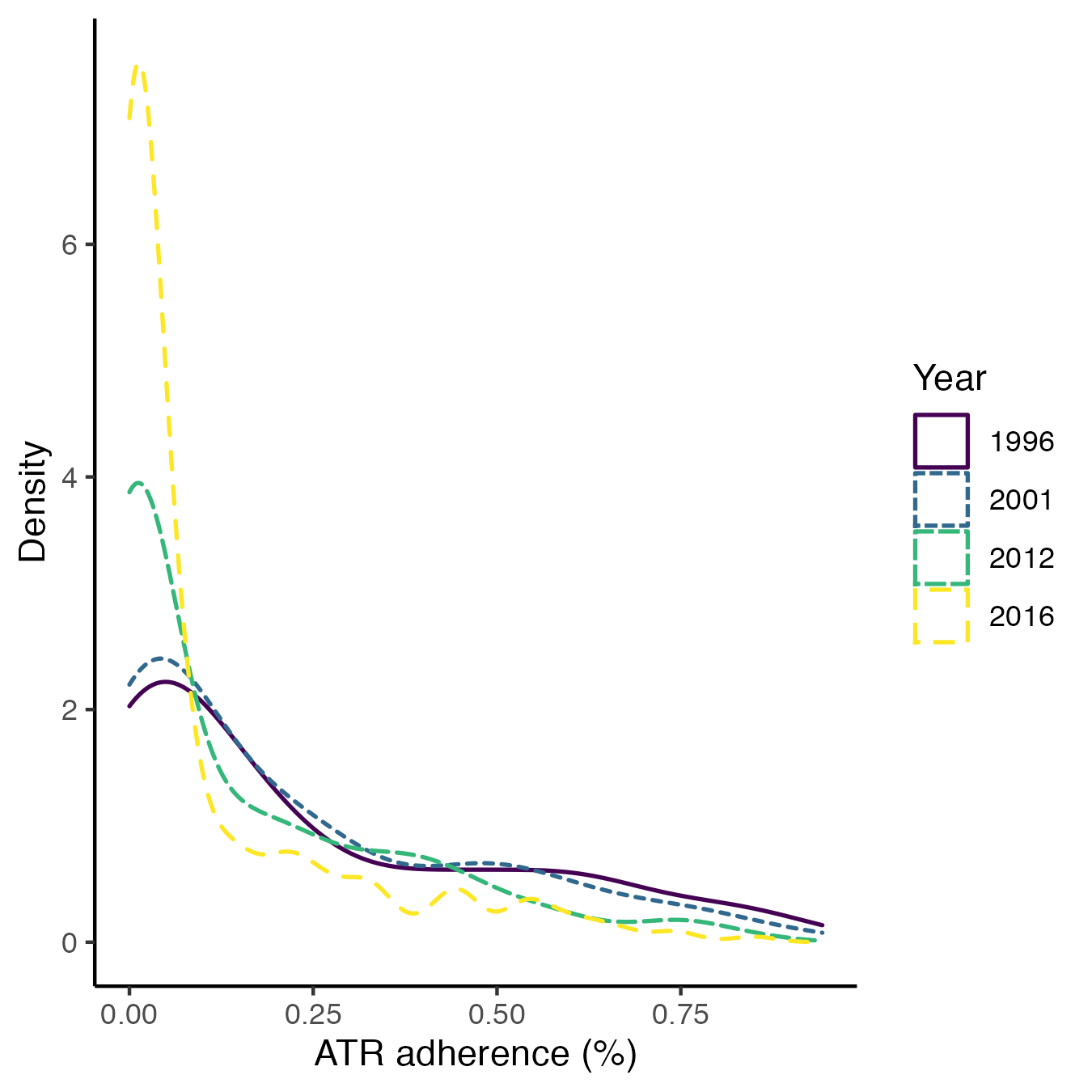
(a)

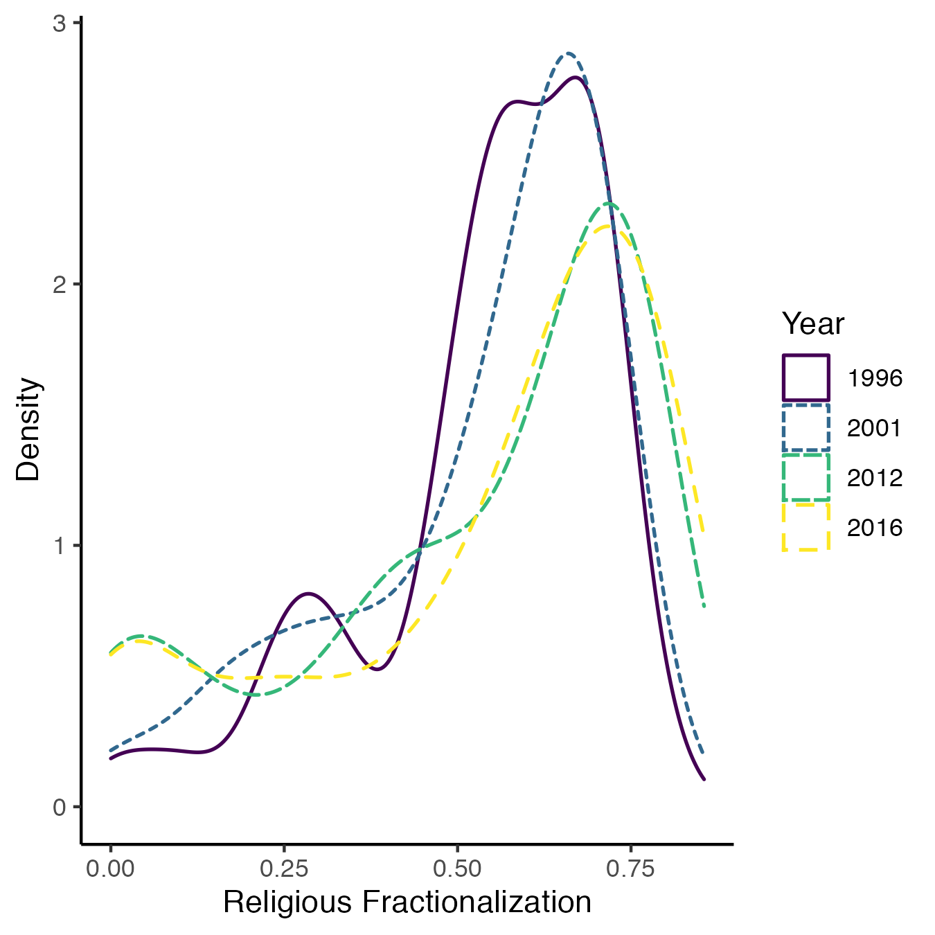
(b)

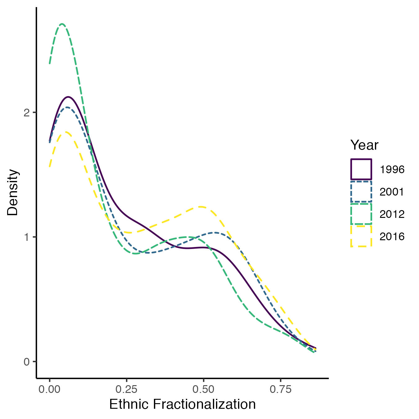
(c)

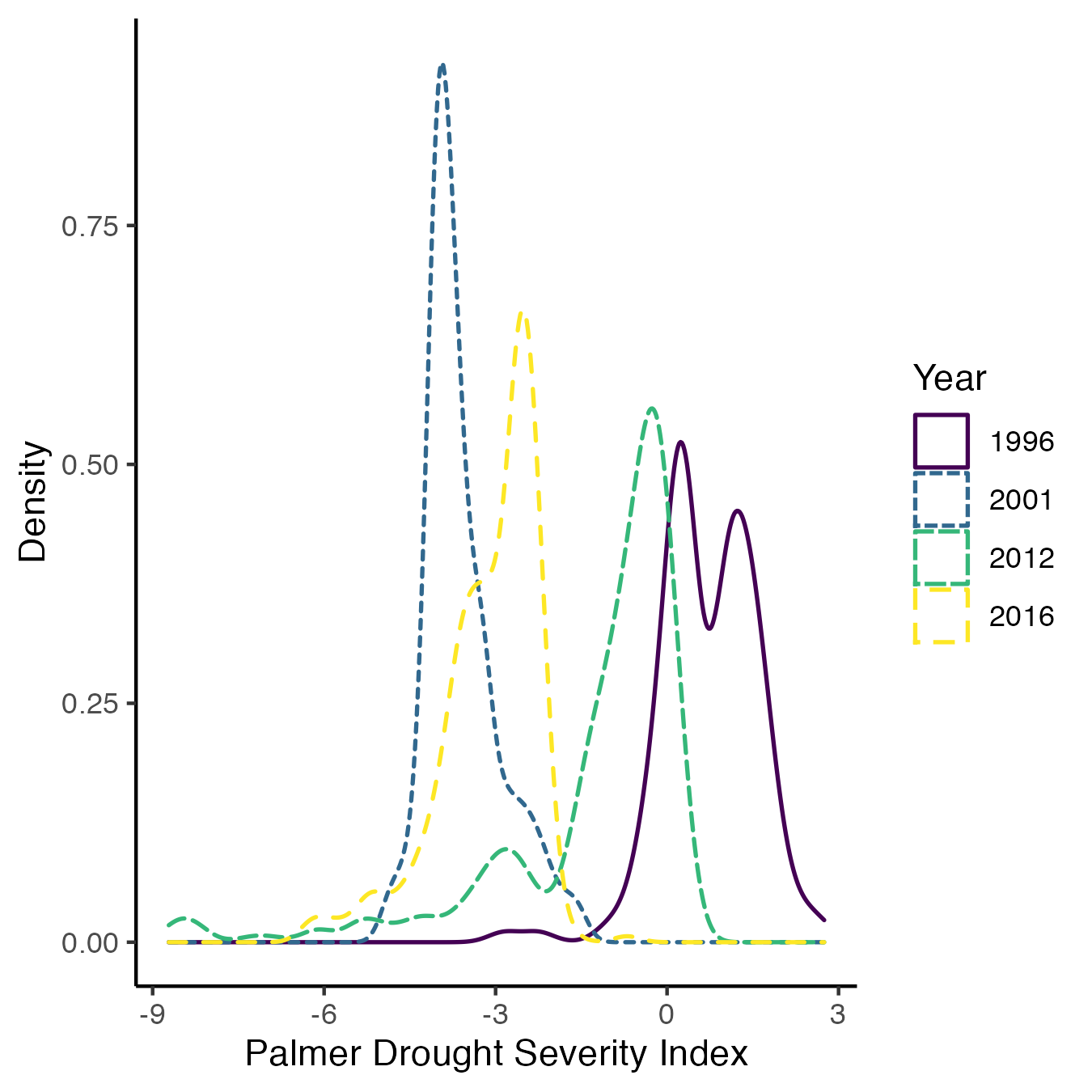
(d)

Figure F.4: Kernel density estimation of the distribution of grid cells by (a) ATR adherence (b) religious fractionalization (c) ethnic fractionalization and (d) Palmer Drought Severity Index, over time.

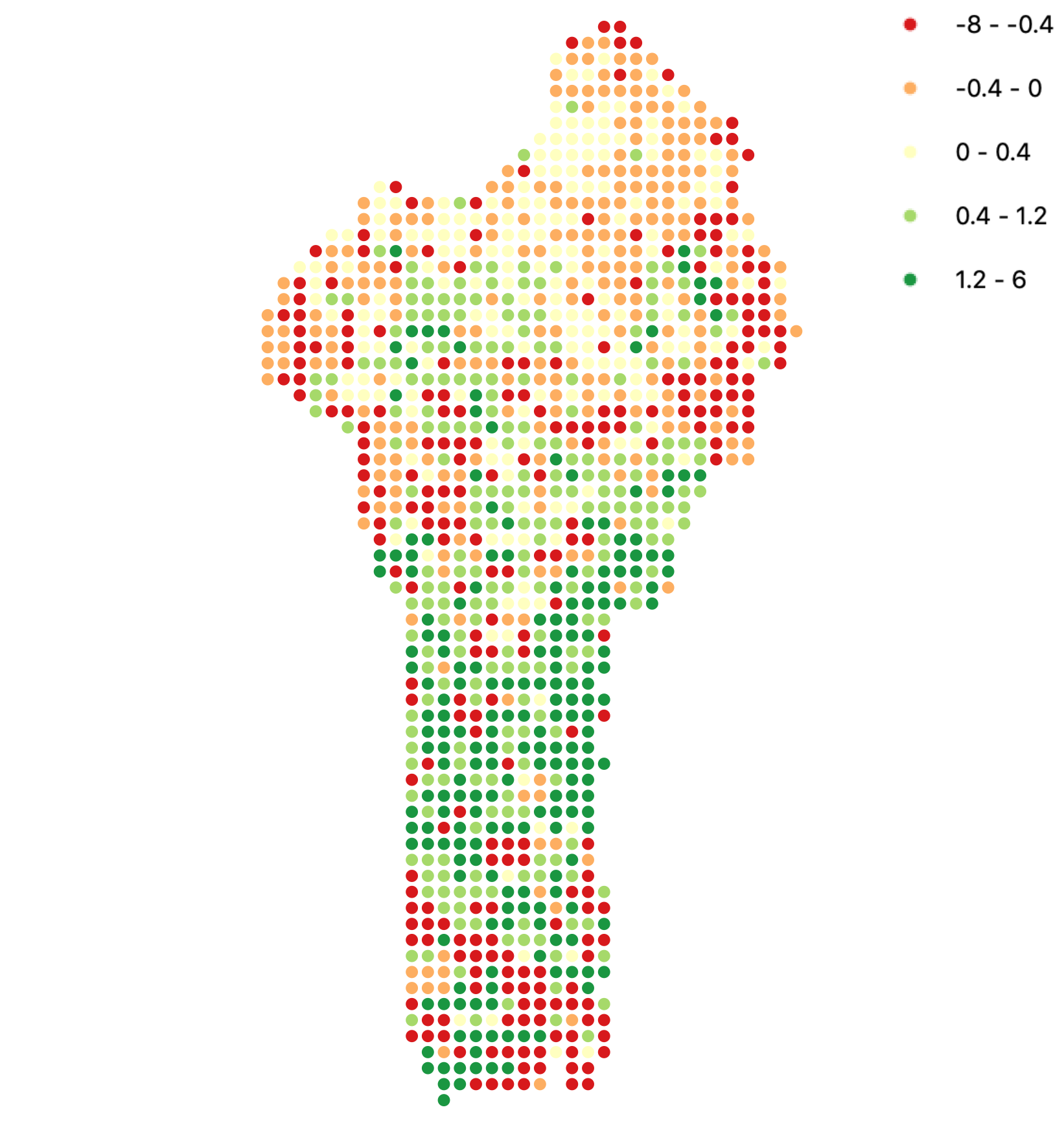
(a) 1996

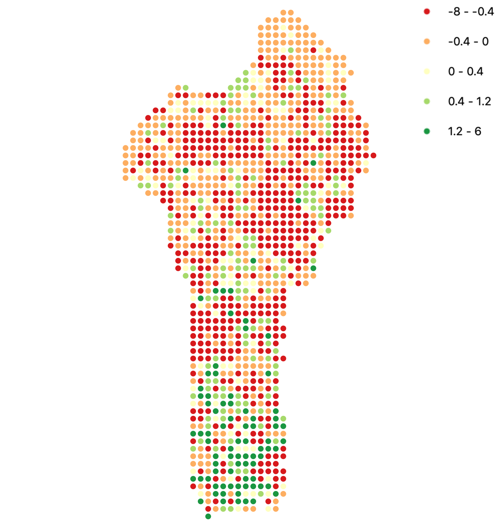
(b) 2016

Figure F.5: Five year average annual change in forest cover represented by the centroids of 10 kms $\times$ 10 kms grid cells.

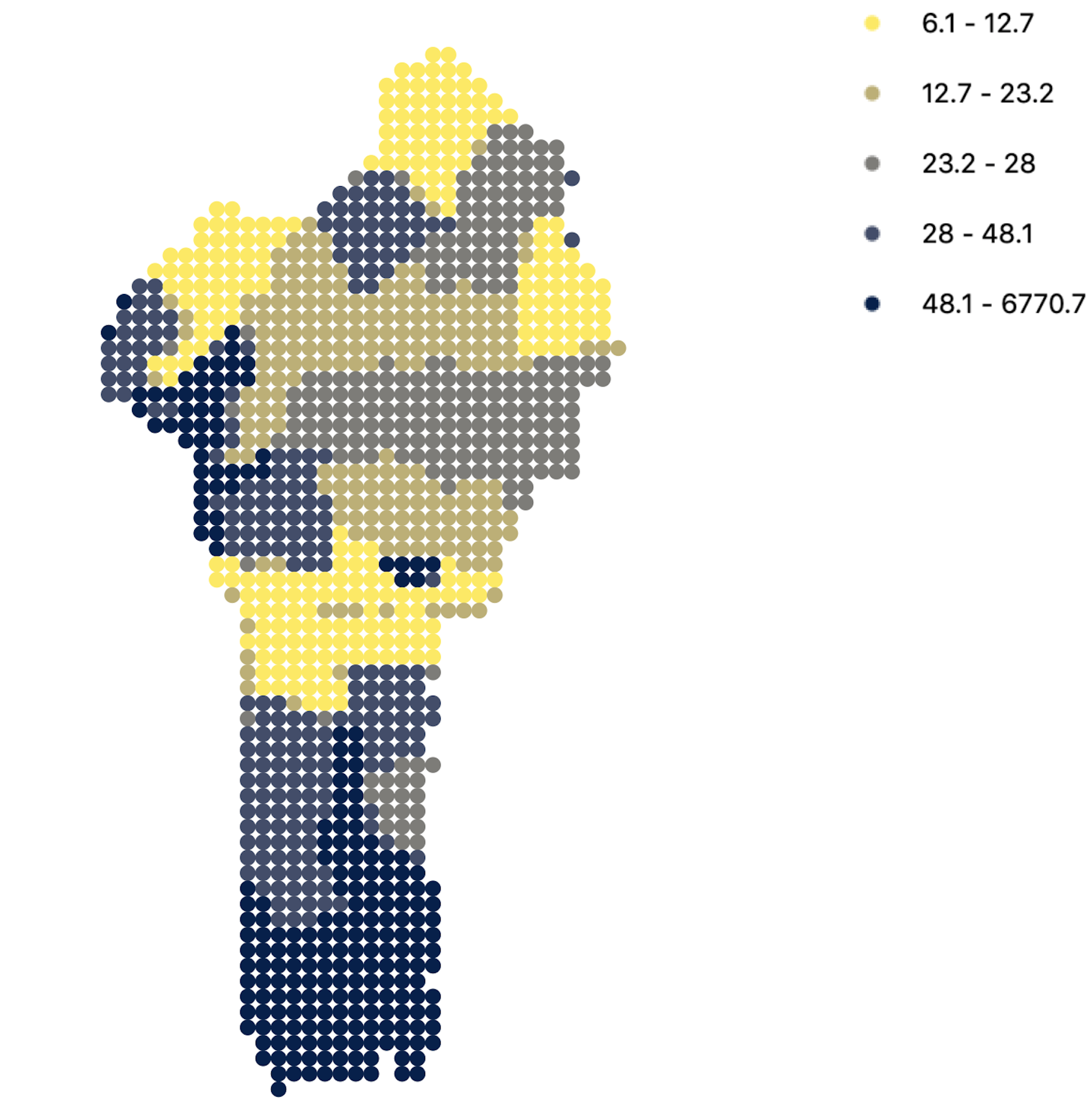
(a) 2000

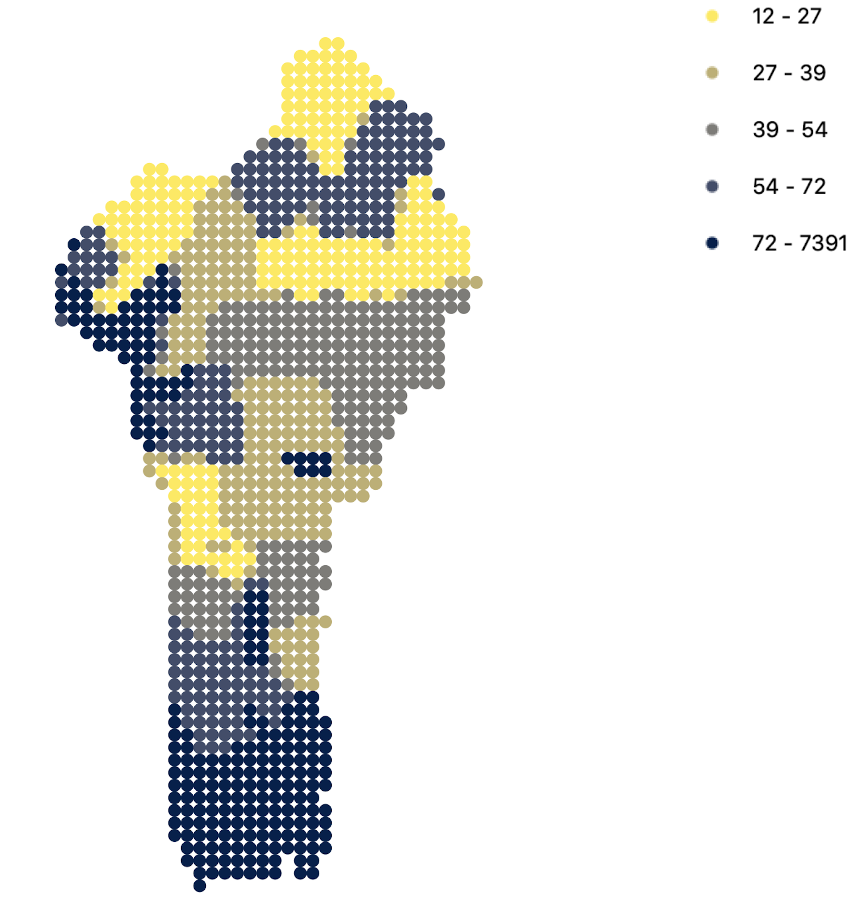
(b) 2015

Figure F.6: Population density by the centroids of 10 kms $\times$ 10 kms grid cells.

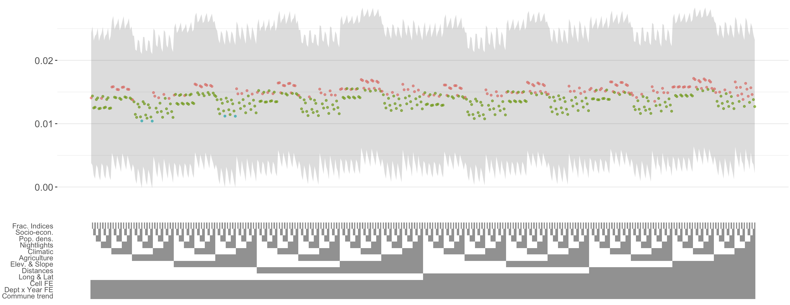
Figure F.7: Robustness of OLS estimates using (16) under every possible combination of groups of control variables while keeping the fixed effects and commune trends as the base controls. Frac. indices includes religious and ethnic fractionalization and socio-econ includes wealth, education and usage of firewood. Pop dens. and nightlights refer to population density and nightlight luminosity. The climatic controls include Palmer Drought Severity Index, precipitation, soil moisture and minimum and maximum temperature. Agricultural controls are soil suitability and area used for harvest for maize, yam, cassava, peanuts, cotton and vegetables. Elev. and slope refer to elevation and terrain slope class. Distances refer to distance to coast, roads, waterways and protected areas. Finally, long. and lat. refer to longitude and latitude to control for spatial trends. Standard errors are robust and clustered at the commune level and 95 percent confidence intervals. Black points are not significant at the ten percent level; blue points are significant at the ten percent level; green points are significant at the five percent level, and red points are significant at the one percent level

Figure F.8: Introducing plausible exogeneity by relaxing exclusion restriction and using the union of confidence intervals (UCI) approach of Conley et al. (2012). Green line refers to the IV estimate in column (6) of Table 1. Figure uses Clarke (2020).

Figure F.9: Light blue represents southern departments of Benin: Atlantique, Couffo, Littoral, Mono, Oueme, Plateau, and Zou. Dark blue represents norther departments: Borgu, Alibori, Atakora, Donga and Collines. The red stars are the location of Protestant and Catholic missions from “Ethnographic Survey of Africa: Showing the Tribes and Languages; also the Stations of Missionary Societies” published by Roome (1925)

Figure F.10: Kingdom of Dahomey 1836 Source: Lovejoy, 2019

(a) Linear RD polynomial $\Delta\text{Cover}^{10y}_{jb}$

(b) Linear RD polynomial $\Delta\text{Cover}^{15y}_{jb}$

(c) Quadratic RD polynomial $\Delta\text{Cover}^{10y}_{jb}$

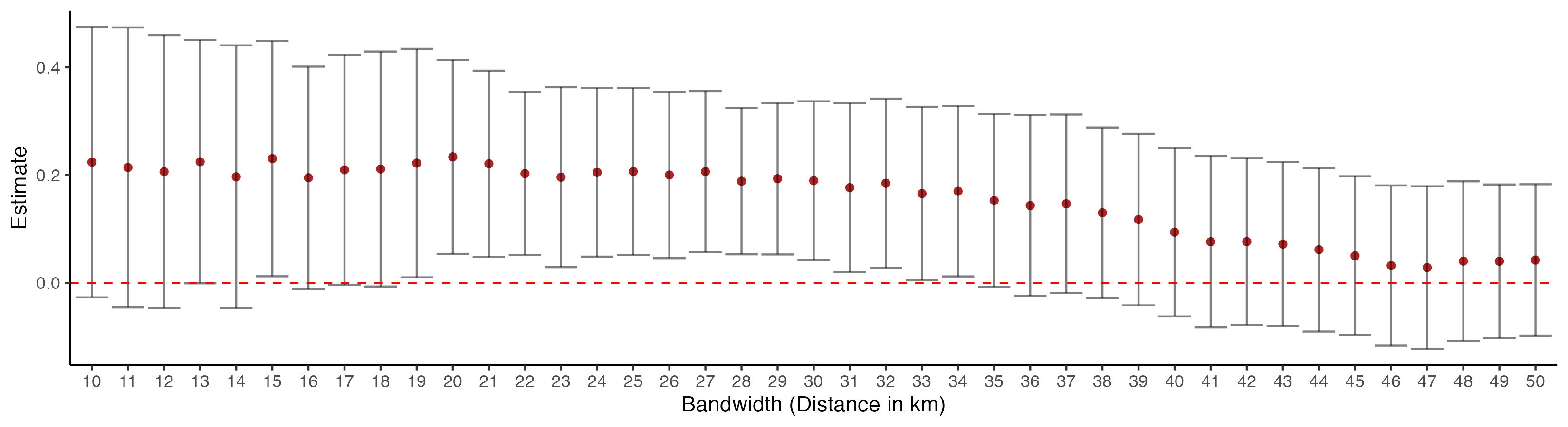
(d) Quadratic RD Polynomial $\Delta\text{Cover}^{15y}_{jb}$

Figure F.11: Robustness of RDD estimates. Figure plots the estimates from equation (18) for different bandwidth values between 10 and 50 km in 1 km increments (horizontal axis). The error bars from the point estimates show 90% confidence intervals, and robust standard errors are clustered at the level of commune.

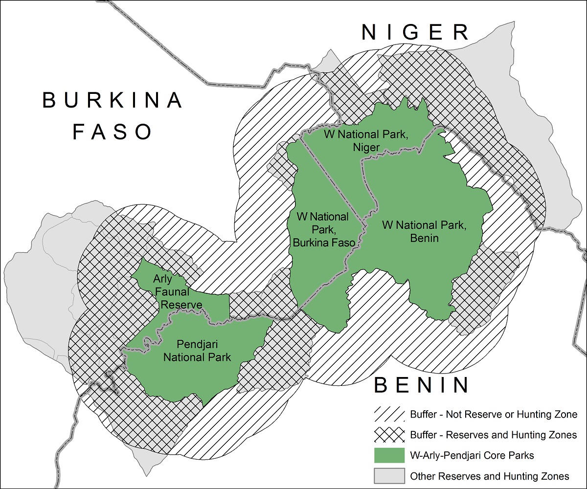
Figure F.12: W-Arly-Pendjari complex and surrounding buffer zones. Source: USGS EROS, accessed October 1, 2022 https://eros.usgs.gov/westafrica/case-study/w-arly-pendjari-transboundary-biosphere-reserve

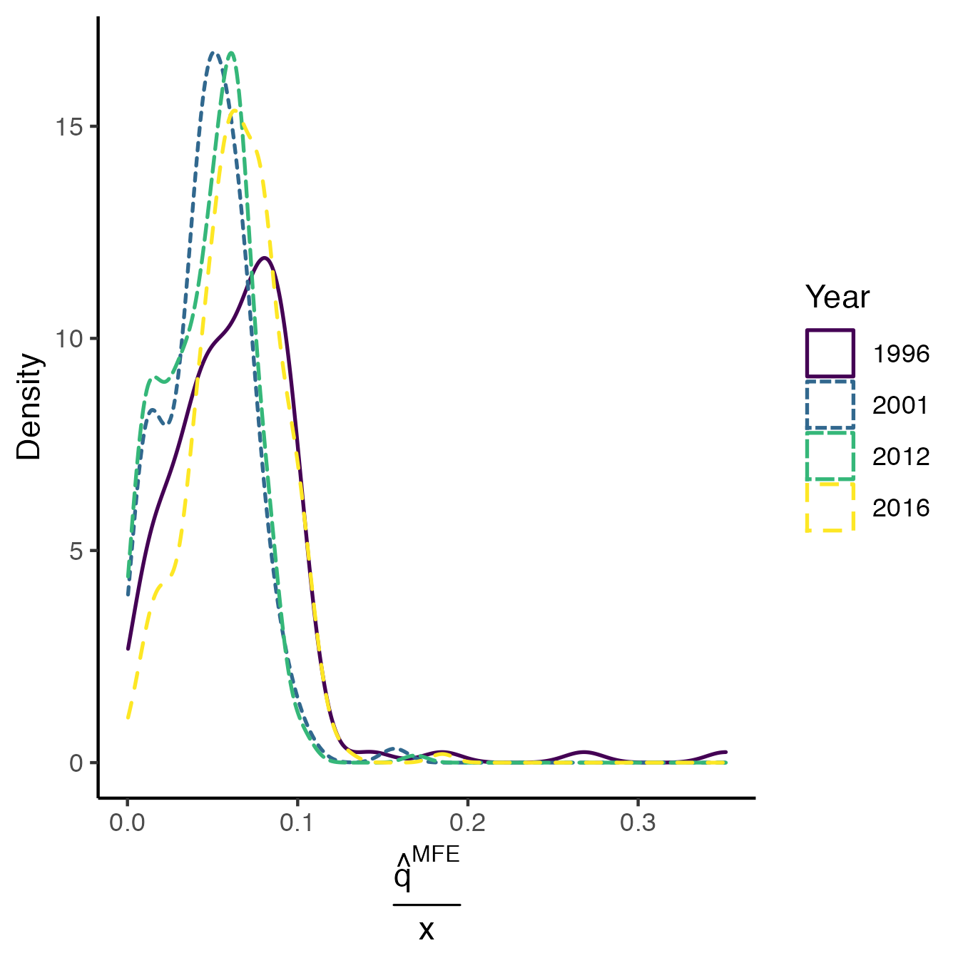
Figure F.13: Density estimation of the distribution of grid cells by $\hat{q}^{MFE}/x$ over time.

Figure F.14: Beliefs distribution fit as a Gamma distribution with shape $k_{a}=0.473$ and rate $\theta_{a}=0.04$

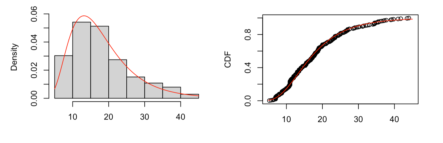
Figure F.15: Equilibrium distribution $p^{a}(x,t)$ at the estimated model parameters (red line) vs. empirical 2016 forest cover distribution (black dots). Histogram vs. predicted density (left panel), theoretical vs. empirical CDF (right panel). Evolution of the theoretical density started at $t_{0}=2012$ in order to evaluate $t=2016$.

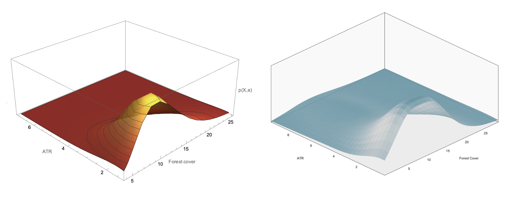
Figure F.16: Predicted (left) vs. observed (right) joint spatial density of ATR and forest cover.

Table F.1: IV Robustness - Spatial Autocorrelation

	OLS				2SLS
	$\Delta\text{Cover}^{5y}_{icdt}$
	(1)	(2)	(3)	(4)	(5)
ATRit	0.005	0.011∗	0.014∗∗	0.013∗∗	0.092∗∗
	(0.003)	(0.006)	(0.007)	(0.007)	(0.044)
Observations	905	905	905	887	887
Cell FE	✓	✓	✓	✓	✓
Year FE	✓	✓	✓	✓	✓
Department $\times$ Year FE		✓	✓	✓	✓
Commune time trend			✓	✓	✓
Baseline controls				✓	✓

• Unit of analysis is 10 kms $\times$ 10 kms grid cell. Conley standard errors with cutoff of 150 kms. Results use equation (16). Climatic controls include: precipitation, Palmer Drought Severity Index and minimum and maximum temperature. Geographic controls include elevation, terrain slope class, soil suitability for agriculture, distance to coast, distance to primary and secondary roads, distance to waterways, distance to protected areas, latitude and longitude - these are interacted with a linear time trend. Socio-economic controls include population density, nighttime lights luminosity, education, wealth, use of firewood as cooking fuel, religious and ethnic fractionalization per grid-cell. Finally the agricultural controls include area used for harvesting of the major subsistence and cash crops in Benin: maize, yam, cassava, cotton, peanuts and vegetables. ^∗p$<$0.1; ^∗∗p$<$0.05; ^∗∗∗p$<$0.01.

Table F.2: Descriptive statistics: 10 kms $\times$ 10kms grid cell characteristics

	Mean	St. Dev.
ATR (%)	16.469	21.671
$\Delta\text{Cover}^{5y}$	$-$0.060	1.225
Precipitation (millimetres)	86.242	11.332
Minimum temperature (Celsius)	22.213	1.245
Maximum temperature (Celsius)	33.008	1.192
Palmer Drought Severity Index	$-$1.916	1.915
Soil moisture (millimetres)	72.044	41.891
Terrain slope class	2.644	0.504
Elevation (metres)	204.525	144.366
Soil suitability for Agriculture	2.904	0.941
Distance to coast (kilometres)	228.124	189.954
Distance to roads (kilometres)	7.669	7.323
Distance to waterways (kilometres)	8.746	7.136
Distance to protected areas (kilometres)	23.715	16.957
Population density	261.849	778.476
Nighttime lights	1.246	4.063
Years of education	2.214	1.784
Rich households (%)	25.272	26.954
Poor households (%)	51.800	30.073
Households owning agricultural land (%)	62.456	29.329
Households using firewood (%)	85.905	20.652
Religious fractionalization	0.534	0.233
Ethnic fractionalization	0.259	0.232
Area harvested for cotton (1000 Ha)	0.148	0.155
Area harvested for yams (1000 Ha)	0.141	0.088
Area harvested for peanuts (1000 Ha)	0.162	0.157
Area harvested for vegetables (1000 Ha)	0.086	0.165
Area harvested for maize (1000 Ha)	1.062	0.708
Area harvested for cassava (1000 Ha)	0.195	0.111

• The table reports descriptive statistics for 10 kms $\times$ 10 kms grid cells. $\Delta\text{Cover}^{5y}$ refers to the 5 year average annual change in forest cover. The following cross-sectional variables are interacted with a linear time trend for estimation: terrain, elevation, soil suitability, distance to coast, distance to roads, distance to waterways and distance to protected areas. Section 4.2 and Appendix E provide detailed definitions as well as the source of each of these variables.

Table F.3: Sub-sampling to southern departments of Benin

	OLS	2SLS	First Stage
	$\Delta\text{Cover}^{5y}_{icdt}$		ATRit
	(1)	(2)	(3)
Panel A:
ATRit	0.025∗∗	0.128∗∗
	(0.012 )	(0.049)
log(Dist. from Nigeria)i			5.979∗∗∗
$\times$			(1.346)
time
K-P F Statistic			19.73
Robust CI		[0.06, 0.20]
Panel B:
ATRit		0.096∗
		(0.055)
log(Dist. from missions)i			0.929∗∗∗
$\times$			(0.276)
time
K-P F Statistic			11.30
Robust CI		[0.01, 0.20]
Observations	372	372	372
Baseline FE & trends	✓	✓	✓
Baseline controls	✓	✓	✓

• Unit of analysis is 10 kms $\times$ 10 kms grid cell. Sample is subset to the southern departments: Zou, Mono, Couffo, Atlantique, Littoral, Oueme and Plateau. Robust standard errors clustered at commune level. 95% confidence intervals based on Chernozhukov and Hansen (2008). Column (1) uses equation (16). Columns (2) and (3) implement IV approach and first stage uses equation (17). Estimation includes cell and department $\times$ year fixed effects and commune time trends. Climatic controls include: precipitation, Palmer Drought Severity Index and minimum and maximum temperature. Geographic controls include elevation, terrain slope class, soil suitability for agriculture, distance to coast, distance to primary and secondary roads, distance to waterways, distance to protected areas, latitude and longitude - these are interacted with a linear time trend. Socio-economic controls include population density, nighttime lights luminosity, education, wealth, use of firewood as cooking fuel, religious and ethnic fractionalization per grid-cell. Finally the agricultural controls include area used for harvesting of the major subsistence and cash crops in Benin: maize, yam, cassava, cotton, peanuts and vegetables. ^∗p$<$0.1; ^∗∗p$<$0.05; ^∗∗∗p$<$0.01.

Table F.4: Local and Global ATR Adherence

	$\Delta\text{Cover}^{5y}_{icdt}$
	OLS		2SLS		OLS interaction
	(1)	(2)	(3)	(4)	(5)	(6)
ATRit	0.011∗∗	0.012∗∗	0.124∗∗	0.098∗∗	0.007	$-$0.0004
	(0.005)	(0.005)	(0.048)	(0.039)	(0.012)	(0.010)
State ATR	$-$0.091∗∗		$-$0.172∗∗		$-$0.090∗∗
	(0.032)		(0.058)		(0.036)
ATR${}^{50kms\;\text{buffer}}$		$-$0.028		$-$0.075∗∗		$-$0.034∗∗
		(0.016)		(0.031)		(0.014)
ATR${}_{it}\times$ State ATR					0.0001
					(0.0004)
ATR${}_{it}\times$ ATR${}^{50kms\;\text{buffer}}$						0.0004
						(0.0003)
Observations	887	887	887	887	887	887
Cell FE	✓	✓	✓	✓	✓	✓
Year FE	✓	✓	✓	✓	✓	✓
Commune time trend	✓	✓	✓	✓	✓	✓
K-P F Statistic			11.3	16.4
Robust CI			[0.05, 0.20]	[0.02, 0.19]

• Unit of analysis is 10 kms $\times$ 10 kms grid cell. Robust standard errors clustered at state level. Estimation uses equation (16) dropping state-by-year fixed effects and introducing an additional explanatory term capturing global ATR adherence. Columns (3) & (4) use the instrument log(Dist. from Nigeria) x time for localized ATR adherence in 10 kms $\times$ 10 kms grid cell. 95% confidence intervals computed as shown by Chernozhukov and Hansen (2008). Columns (5) & (6) introduce an interaction between localized adherence ATR_it and global adherence variable. Climatic controls include: precipitation, Palmer Drought Severity Index and minimum and maximum temperature. Geographic controls include elevation, terrain slope class, soil suitability for agriculture, distance to coast, distance to primary and secondary roads, distance to waterways, distance to protected areas, latitude and longitude - these are interacted with a linear time trend. Socio-economic controls include population density, nighttime lights luminosity, education, wealth, use of firewood as cooking fuel, religious and ethnic fractionalization per grid-cell. Finally the agricultural controls include area used for harvesting of the major subsistence and cash crops in Benin: maize, yam, cassava, cotton, peanuts and vegetables. ^∗p$<$0.1; ^∗∗p$<$0.05; ^∗∗∗p$<$0.01.

Table F.5: Spatial RDD - Balance checks

	Estimate	Std.error
	(1)	(2)
Soil suitability	0.149	0.113
Slope	0.196	0.199
Elevation	-6.058	8.743
Pop. Density	0.008	0.079
Dist. to roads	0.19	0.223
Dist. to waterways	-0.089	0.207
Precipitation	-1.002	1.095
Temperature	-0.008	0.058
Croplands 1600 AD	-5.981	5.943
Grazing 1600 AD	-0.674	2.305
Nighttime lights	-0.042	0.205

• Results use equation (18) with linear RD polynomial and bandwidth of 30 kms. Robust standard errors clustered at commune level. Appendix E provide detailed definitions as well as the source of each of these variables.

Table F.6: Spatial RDD Robustness - Spatial Autocorrelation

	$\Delta\text{Cover}^{5y}_{jb}$	$\Delta\text{Cover}^{10y}_{jb}$	$\Delta\text{Cover}^{15y}_{jb}$
	(1)	(2)	(3)
Linear RD Polynomial:
Dahomeyj	0.278	0.344∗∗	0.175∗∗
	(0.195)	(0.162)	(0.085)
Quadratic RD Polynomial:
Dahomeyj	0.137	0.342∗	0.190∗∗∗
	(0.310)	(0.183)	(0.062)
Observations	439	439	439
Segment fixed effects	✓	✓	✓

• Unit of analysis is 5.6 kms $\times$ 5.6 kms grid cell. Conley standard errors with cutoff of 50 kms. Results use equation (18) and control for log(dist. from coast). All estimations use a bandwidth of 30 kms. ^∗p$<$0.1; ^∗∗p$<$0.05; ^∗∗∗p$<$0.01.

Table F.7: Pre-colonial ethnic characteristics from the Ethnographic Atlas

	Fon	Oyo-Yoruba
Characteristics	(1)	(2)
Jurisdictional hierarchy of local community [EA032]	Large States	Large States
Class differentiation: primary [EA066]	Dual stratification	Complex stratification
Settlement patterns [EA030]	Villages/towns	Villages/towns

• Information from Murdock (1967) Ethnographic Atlas. Values in the parenthesis refer to the variable number. EA032 refers to the number of jurisdictional levels beyond the local community and also provides a measure of political complexity. EA066 refers to the degree and type of class differentiation, excluding purely political and religious statuses. EA030 refers to the prevailing type of settlement pattern.

Table F.8: Spatial noise randomization inference

	Coefficient	Directional	Effective	Structure	Randomized	Standard
	$\zeta$	$R^{2}$	range	$\rho$	p value	error
	(1)	(2)	(3)	(4)	(5)	(6)
$\Delta\text{Cover}^{10y}_{jb}$
	0.344	0.039	80	0.80	0.040	0.168
$\Delta\text{Cover}^{15y}_{jb}$
	0.175	0.039	80	0.80	0.091	0.104

• Spatial structure of the components of the explanatory variable Dahomey_j. Results use equation (18) with linear RD polynomial and bandwidth of 30 kms. Unit of analysis is 5.6 kms $\times$ 5.6 kms grid cell. Directional $R^{2}$ gives the explanatory power of a regression of the variable on spatial dimensions i.e. longitude and latitude. Effective range is the distance in kilometres where the correlation between locations of the detrended variable has fallen to 0.14; and structure $\rho$ is its spatial signal to noise ratio. The smoothness parameter used is $\kappa=1.5$ which is the exponential decay of correlation.

Table F.9: Mechanism: Land degradation & agricultural expansion

	$\text{Exp}^{5y}_{it}$		$\text{Degr}^{5y}_{it}$
	(1)	(2)	(3)	(4)
ATRit	$-$0.003		$-$0.001
	(0.002)		(0.002)
ATR${}^{q(75)}_{it}$		$-$0.221∗∗		0.080
		(0.091)		(0.074)
Observations	887	887	887	887
Baseline FE & trends	✓	✓	✓	✓
Baseline controls	✓	✓	✓	✓

• Unit of analysis is 10 kms $\times$ 10 kms grid cell. Standard errors are clustered at commune level. Estimation includes cell and department $\times$ year fixed effects and commune time trends. Climatic controls include: precipitation, soil moisture, Palmer Drought Severity Index and minimum and maximum temperature. Geographic controls include soil suitability, distance to coast, distance to primary and secondary roads, distance to waterways, elevation, terrain slope, distance to protected areas, latitude and longitude - these are interacted with a time trend. Economic and demographic controls include population density, nighttime lights luminosity, education, wealth, use of firewood as cooking fuel, religious and ethnic fractionalization per grid-cell. Finally the agricultural controls include area used for harvesting of the major subsistence and cash crops in Benin: Maize, Yam, Cassava, Cowpeas, Peanuts, Cotton and vegetables. ^∗p$<$0.1; ^∗∗p$<$0.05; ^∗∗∗p$<$0.01.

Appendix G Sustainable Agricultural Practices

We provide motivating evidence on the usage of sustainable agricultural practices by ATR households. We use the Enquête Harmonisée sur le Conditions de Vie des Ménages (EHCVM) 2018-2019 which is a nationally representative household survey, conducted in two waves with each wave covering half of the sample. The first wave was fielded between October 2018 and December 2018, while the second wave occurred between April and July 2019. The two-wave approach was chosen to account for seasonality of consumption. The survey uses two main survey instruments. The first instrument is a household/individual questionnaire, and the second is a community-level questionnaire. The former provides detailed information on socio-demographic characteristic, assets, transfers, shocks, safety nets, agricultural lands, inputs and crops, livestock, farming equipment, fishing, and relative poverty. The data is available at https://microdata.worldbank.org/index.php/catalog/4291.

The survey, however, does not provide GPS coordinates and thus we are unable to match it to the spatially explicit estimations. Nevertheless, it is sufficient to provide suggestive evidence. Additional details about EHCVM dataset are provided in Appendix E. Focusing on three soil fertility management practices (i) intercropping and agroforestry (ii) no tillage and (iii) use of organic fertilizers (household and animal waste) we estimate the following:

$$\text{S}_{phc} =\psi\text{ATR}_{h}+\boldsymbol{\Lambda}\textbf{Z}_{p}+\boldsymbol{\Xi}\textbf{H}_{h}+\alpha_{c}+\epsilon_{phc}$$ (32)

where $\text{S}_{phc}$ is a dummy variable which takes the value 1 if the household $h$ in cluster $c$ implements the sustainable agricultural practice S in plot $p$, and 0 otherwise. Similarly, $\text{ATR}_{h}$ is a dummy variable taking the value 1 if the head of the household is an ATR adherent. Lastly, $\textbf{Z}_{p}$ and $\textbf{H}_{h}$ are vectors of plot and household characteristics, and $\alpha_{c}$ captures cluster fixed effect. As seen in Figure G.1 we find that ATR households are more likely to adopt sustainable farming practices.

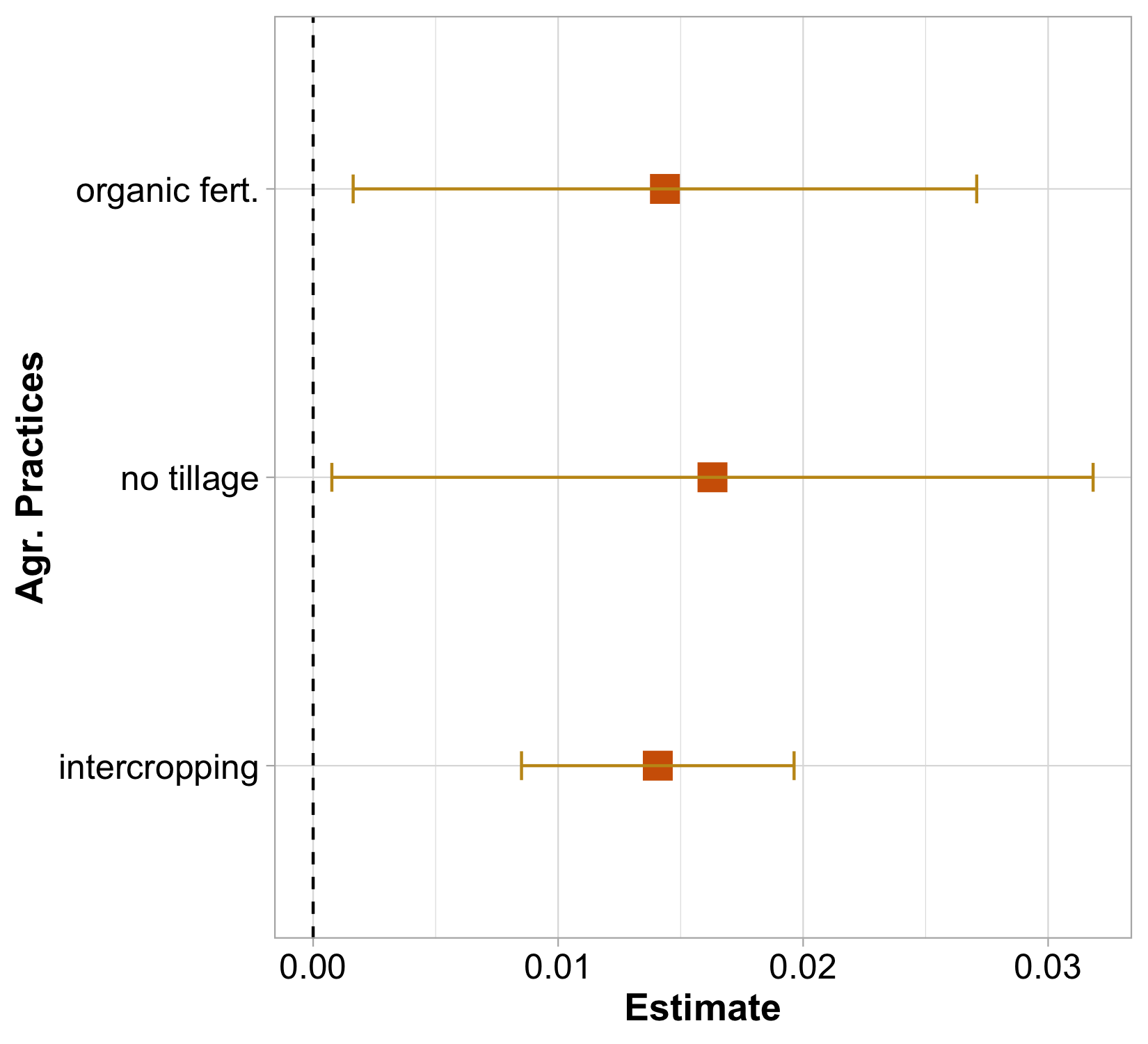
Figure G.1: ATR and sustainable agricultural practices. Results use equation (32). Unit of analysis is plot. Standard errors are bootstrapped at region level. Confidence interval of 90%. Plot characteristics include area in hectares, land tenure, topography, fertility as perceived by farmer. Household characteristics include size, access to credit via tontine, livestock herd, head’s age, gender and education.

Appendix H Social Capital

Social capital in a community generates positive externalities for members of a group and these are achieved through shared trust, norms, and values based on social networks and associations (Aghion and Durlauf, 2005; Guiso et al., 2011). Since forests are common (public) goods for local communities, social capital often plays an important role in tackling issues of deforestation and resource degradation as it lowers the transaction costs of working together, facilitates cooperation and provides confidence to invest in collective action, knowing that others will do the same. (Katz, 2000; Ostrom et al., 2002; Pretty, 2003; Alix-Garcia et al., 2018; Alesina et al., 2019). Religion has been shown to be an important source of accumulation of social capital as it can provide shared norms used to achieve cooperative ends and a platform for building social bonds. Religious activity and participation induce altruism, trust, and willingness to join efforts with other members of the religious group (Guiso et al., 2003; i Miquel et al., 2012; Deller et al., 2018).

Therefore, a likely mechanism via which ATR adherence has a positive impact on forest cover change may be due to social capital formation leading to greater conservation efforts and efficient monitoring. We use five variables to proxy for social capital: first is residential stability - $Res.Stab_{it}$ - measured using DHS as the percentage of individuals within a grid cell $i$ at time $t$ who have always lived there. This variable captures social cohesion and may be indicative of the strength of locally based networks and associations (Forrest and Kearns, 2001). The remaining four are widely used measures from Afrobarometer surveys at the commune level: $Trust_{ct}$ - generalized trust toward others, $Comm.Part_{ct}$ - participation in community meetings, $Issues_{ct}$ - collectively raising an issue and $Member_{ct}$ - active membership of a religious group. Appendix E provides further details on the construction of these variables. We estimate equation (16) with social capital proxy as the outcome variable and present the results in Table H.1. Surprisingly, we find that ATR adherence is not significantly correlated to any indicators of social capital.

Discerning the ATR beliefs and structure can shed light on understanding these results. ATR, compared to Christianity, is less organized and places less emphasis on frequency of institutional observance and participation. For example, attending weekly church service provides a platform to build networks and associations and increase mutual trust. The absence of this requirement may explain the results partly. However, it would be prudent to pay closer attention to the components of social capital. According to Putnam (2015) both norms and networks are key elements and the distinction between the two corresponds roughly to Uphoff (2000)’s distinction between cognitive and structural manifestations of social capital. Generally, empirical proxies such as the ones used here broadly capture the informational advantages of networks. It would seem that although ATR may lack centralization and network building it is in fact rich in social norms. According to Mbiti (1990) to maintain social cohesion within the community, which includes the living and the spirits, every African society retains a moral code containing customs, regulations, and taboos. This is also consistent with Iyer (2018)’s observation that non European religions often place more emphasis on morality and rituals than religious doctrines.

Lastly, Table H.1 also presents results on fractionalization indices as they have been shown to be key for social capital. Consistent with results presented by and Alesina et al. (2003) and Putnam (2007), we find ethnic fractionalization to be significant and negatively correlated to residential stability, generalized trust and community participation. Interestingly religious fractionalization, which is a good proxy for tolerance and plurality, is negatively correlated with active membership of a religious groups.

Table H.1: Mechanism: Social capital

	Res.Stabit	Trustct	Comm.Partct	Issuesct	Memberct
	(1)	(2)	(3)	(4)	(5)
ATRit	$-$0.008	0.013	$-$0.009	0.013	0.007
	(0.040)	(0.020)	(0.036)	(0.033)	(0.030)
Religious fractionalization	$-$6.687	0.451	3.050	$-$5.394	$-$8.264∗∗
	(4.063)	(1.497)	(3.590)	(3.360)	(3.062)
Ethnic fractionalization	$-$6.911∗∗	$-$3.442∗∗	$-$3.636∗	$-$0.790	$-$1.471
	(3.339)	(1.231)	(2.164)	(2.050)	(2.363)
Observations	788	580	698	698	698
Baseline FE & trends	✓	✓	✓	✓	✓
Baseline controls	✓	✓	✓	✓	✓

• Results use equation (16). Robust standard errors clustered at commune level. Column (1) Res.Stab_it refers to residential stability, column (2) Trust_ct refers to generalized trust, column (3) Comm.Part_ct refers to participation in community meetings, column (4) Issues_ct refers to collectively raising an issue and column (5) Member_ct refers to membership of a religious group. Estimation includes cell and department $\times$ year fixed effects and commune time trends. Climatic controls include: precipitation, Palmer Drought Severity Index and minimum and maximum temperature. Geographic controls include elevation, terrain slope class, soil suitability for agriculture, distance to coast, distance to primary and secondary roads, distance to waterways, distance to protected areas, latitude and longitude - these are interacted with a linear time trend. Socio-economic controls include population density, nighttime lights luminosity, education, wealth, use of firewood as cooking fuel, religious and ethnic fractionalization per grid-cell. Finally the agricultural controls include area used for harvesting of the major subsistence and cash crops in Benin: maize, yam, cassava, cotton, peanuts and vegetables. ^∗p$<$0.1; ^∗∗p$<$0.05; ^∗∗∗p$<$0.01. .

Appendix I Images from Benin

Figure I.1: Monument of King Béhanzin of Dahomey (reigned 1889–1904, defeated by the French in 1892) at the entrance to Abomey. The inscription reads ”I will never sign any treaty which might alienate the independence of the land of my ancestors.” Source: Digital Histories, accessed August 29, 2022 https://digitalhistories.kennesaw.edu/items/show/78

Figure I.2: Ouidah92 poster in a collage of concert posters in the home of the Haitian band Boukman Eksperyans. Source: Rush (2001)

Figure I.3: La Porte du Non-Retour (The Door of No Return) at the port in Ouidah. Source: ©jbdodane.com

References

- Acemoglu and Jensen (2015) Acemoglu, D. and M. K. Jensen (2015). Robust comparative statics in large dynamic economies. Journal of Political Economy 123(3), 587–640.
- Aderibigbe and Falola (2022) Aderibigbe, I. S. and T. Falola (2022). The palgrave handbook of african traditional religion.
- Aghion and Durlauf (2005) Aghion, P. and S. Durlauf (2005). Handbook of economic growth. Elsevier.
- Akinwumi (1999) Akinwumi, O. (1999). Oral traditions and the political history of borgu. Anthropos (H. 1./3), 215–221.
- Alesina et al. (2003) Alesina, A., A. Devleeschauwer, W. Easterly, S. Kurlat, and R. Wacziarg (2003). Fractionalization. Journal of Economic growth 8(2), 155–194.
- Alesina et al. (2019) Alesina, A., C. Gennaioli, and S. Lovo (2019). Public goods and ethnic diversity: Evidence from deforestation in indonesia. Economica 86(341), 32–66.
- Alesina and Giuliano (2015) Alesina, A. and P. Giuliano (2015). Culture and institutions. Journal of economic literature 53(4), 898–944.
- Alidou (2021) Alidou, S. (2021). Beliefs and investment in child human capital: case study from benin. The Journal of Development Studies 57(1), 88–105.
- Alix-Garcia et al. (2018) Alix-Garcia, J. M., K. R. Sims, V. H. Orozco-Olvera, L. E. Costica, J. D. Fernández Medina, and S. Romo Monroy (2018). Payments for environmental services supported social capital while increasing land management. Proceedings of the National Academy of Sciences 115(27), 7016–7021.
- Alonso et al. (2016) Alonso, E. B., R. Houssa, and M. Verpoorten (2016). Voodoo versus fishing committees: The role of traditional and contemporary institutions in fisheries management. Ecological Economics 122, 61–70.
- Altonji et al. (2005) Altonji, J. G., T. E. Elder, and C. R. Taber (2005). Selection on observed and unobserved variables: Assessing the effectiveness of catholic schools. Journal of political economy 113(1), 151–184.
- Araújo et al. (2022) Araújo, D., B. Carrillo, and B. Sampaio (2022). Economic production and the spread of supernatural beliefs.
- Asiwaju (1985) Asiwaju, A. I. (1985). Partitioned Africans: Ethnic relations across Africa’s international boundaries, 1884-1984. C. Hurst & Co. Publishers.
- Barba and Jaimovich (2022) Barba, F. M. and D. Jaimovich (2022). Ethnic diversity and forest commons. World Development 158, 105986.
- Bentzen and Gokmen (2022) Bentzen, J. S. and G. Gokmen (2022). The power of religion. Journal of Economic Growth, 1–34.
- Berkes (2017) Berkes, F. (2017). Sacred ecology. Routledge.
- Blier (1994) Blier, S. P. (1994). The anatomy of architecture: ontology and metaphor in Batammaliba architectural expression. University of Chicago Press.
- Boko (2017) Boko, H. N. K. (2017). The evolution of cultural and natural management systems with the waterlogged villages in benin. In Managing Heritage in Africa, pp. 97–109. Routledge.
- Brock and Durlauf (2001) Brock, W. A. and S. N. Durlauf (2001). Discrete choice with social interactions. The Review of Economic Studies 68(2), 235–260.
- Brouwers (1993) Brouwers, J. H. A. M. (1993). Rural people’s response to soil fertility decline: the Adja case (Benin). Wageningen University and Research.
- Carvalho et al. (2019) Carvalho, J.-P., S. Iyer, and J. Rubin (2019). Advances in the Economics of Religion. Springer.
- Chernozhukov and Hansen (2008) Chernozhukov, V. and C. Hansen (2008). The reduced form: A simple approach to inference with weak instruments. Economics Letters 100(1), 68–71.
- Claffey (2007) Claffey, P. (2007). Christian churches in Dahomey-Benin: a study of their socio-political role. Brill.
- Clarke (2020) Clarke, D. (2020). Plausexog: Stata module to implement conley et al’s plausibly exogenous bounds.
- Conley (1999) Conley, T. G. (1999). Gmm estimation with cross sectional dependence. Journal of econometrics 92(1), 1–45.
- Conley et al. (2012) Conley, T. G., C. B. Hansen, and P. E. Rossi (2012). Plausibly exogenous. Review of Economics and Statistics 94(1), 260–272.
- Coşgel et al. (2019) Coşgel, M. M., J. Hwang, T. J. Miceli, and S. Yıldırım (2019). Religiosity: Identifying the effect of pluralism. Journal of Economic Behavior & Organization 158, 219–235.
- Dell et al. (2018) Dell, M., N. Lane, and P. Querubin (2018). The historical state, local collective action, and economic development in vietnam. Econometrica 86(6), 2083–2121.
- Deller et al. (2018) Deller, S. C., T. Conroy, and B. Markeson (2018). Social capital, religion and small business activity. Journal of Economic Behavior & Organization 155, 365–381.
- Dohmen et al. (2011) Dohmen, T., A. Falk, D. Huffman, U. Sunde, J. Schupp, and G. G. Wagner (2011). Individual risk attitudes: Measurement, determinants, and behavioral consequences. Journal of the european economic association 9(3), 522–550.
- Dupuis (1998) Dupuis, P. P.-H. (1998). Histoire de l’église du bénin, tome 1, le temps des semeurs (1494–1901).
- Falen (2018) Falen, D. J. (2018). African science: Witchcraft, vodun, and healing in Southern Benin. University of Wisconsin Press.
- Filippini and Wekhof (2021) Filippini, M. and T. Wekhof (2021). The effect of culture on energy efficient vehicle ownership. Journal of Environmental Economics and Management 105, 102400.
- Forrest and Kearns (2001) Forrest, R. and A. Kearns (2001). Social cohesion, social capital and the neighbourhood. Urban studies 38(12), 2125–2143.
- Fukuyama (1996) Fukuyama, F. (1996). Trust: The social virtues and the creation of prosperity. Simon and Schuster.
- Gabaix et al. (2016) Gabaix, X., J.-M. Lasry, P.-L. Lions, and B. Moll (2016). The dynamics of inequality. Econometrica 84(6), 2071–2111.
- Gaoue and Ticktin (2009) Gaoue, O. G. and T. Ticktin (2009). Fulani knowledge of the ecological impacts of khaya senegalensis (meliaceae) foliage harvest in benin and its implications for sustainable harvest. Economic botany 63(3), 256–270.
- Gelman and Imbens (2019) Gelman, A. and G. Imbens (2019). Why high-order polynomials should not be used in regression discontinuity designs. Journal of Business & Economic Statistics 37(3), 447–456.
- Gennaioli and Rainer (2007) Gennaioli, N. and I. Rainer (2007). The modern impact of precolonial centralization in africa. Journal of Economic Growth 12(3), 185–234.
- Gershman (2016) Gershman, B. (2016). Witchcraft beliefs and the erosion of social capital: Evidence from sub-saharan africa and beyond. Journal of Development Economics 120, 182–208.
- Glaeser and Scheinkman (2000) Glaeser, E. L. and J. A. Scheinkman (2000). Non-market interactions.
- Grim (2001) Grim, J. A. (2001). Indigenous traditions and ecology. Harvard University Press Cambridge, MA.
- Gruber (2005) Gruber, J. H. (2005). Religious market structure, religious participation, and outcomes: Is religion good for you? The BE Journal of Economic Analysis & Policy 5(1).
- Guéant et al. (2011) Guéant, O., J.-M. Lasry, and P.-L. Lions (2011). Mean field games and applications. In Paris-Princeton lectures on mathematical finance 2010, pp. 205–266. Springer.
- Guiso et al. (2003) Guiso, L., P. Sapienza, and L. Zingales (2003). People’s opium? religion and economic attitudes. Journal of monetary economics 50(1), 225–282.
- Guiso et al. (2006) Guiso, L., P. Sapienza, and L. Zingales (2006). Does culture affect economic outcomes? Journal of Economic perspectives 20(2), 23–48.
- Guiso et al. (2011) Guiso, L., P. Sapienza, and L. Zingales (2011). Civic capital as the missing link. Handbook of social economics 1, 417–480.
- Hall and Heyde (2014) Hall, P. and C. C. Heyde (2014). Martingale limit theory and its application. Academic press.
- Handberg and Angelsen (2015) Handberg, Ø. N. and A. Angelsen (2015). Experimental tests of tropical forest conservation measures. Journal of Economic Behavior & Organization 118, 346–359.
- Hayo and Vollan (2012) Hayo, B. and B. Vollan (2012). Group interaction, heterogeneity, rules, and co-operative behaviour: Evidence from a common-pool resource experiment in south africa and namibia. Journal of Economic Behavior & Organization 81(1), 9–28.
- Hilary and Hui (2009) Hilary, G. and K. W. Hui (2009). Does religion matter in corporate decision making in america? Journal of financial economics 93(3), 455–473.
- Horsthemke (2015) Horsthemke, K. (2015). Animals and African ethics. Springer.
- i Miquel et al. (2012) i Miquel, G. P., N. Qian, and Y. Yao (2012). Social fragmentation, public goods and elections: Evidence from china. Technical report, National Bureau of Economic Research.
- Iannaccone (1998) Iannaccone, L. R. (1998). Introduction to the economics of religion. Journal of economic literature 36(3), 1465–1495.
- Iannaccone and Bainbridge (2009) Iannaccone, L. R. and W. S. Bainbridge (2009). Economics of religion. In The Routledge Companion to the Study of Religion, pp. 475–489. Routledge.
- Idowu (1973) Idowu, E. B. (1973). African traditional religion: A definition. Orbis Books.
- Iyer (2016) Iyer, S. (2016). The new economics of religion. Journal of Economic Literature 54(2), 395–441.
- Iyer (2018) Iyer, S. (2018). The economics of religion in India. Harvard University Press.
- Jedwab et al. (2022) Jedwab, R., F. Meier zu Selhausen, and A. Moradi (2022). The economics of missionary expansion: evidence from africa and implications for development. Journal of Economic Growth 27(2), 149–192.
- Jedwab et al. (2021) Jedwab, R., F. M. zu Selhausen, and A. Moradi (2021). Christianization without economic development: Evidence from missions in ghana. Journal of Economic Behavior & Organization 190, 573–596.
- Johnson et al. (2011) Johnson, K. A., E. D. Hill, and A. B. Cohen (2011). Integrating the study of culture and religion: Toward a psychology of worldview. Social and Personality Psychology Compass 5(3), 137–152.
- Juhé-Beaulaton (2010) Juhé-Beaulaton, D. (2010). Forêts sacrées et sanctuaires boisés: des créations culturelles et biologiques (Burkina Faso, Togo, Bénin). KARTHALA Editions.
- Kahn (2011) Kahn, J. (2011). Policing ‘evil’: state-sponsored witch-hunting in the people’s republic of bénin. Journal of Religion in Africa 41(1), 4–34.
- Katic and Ellis (2018) Katic, P. and T. Ellis (2018). Risk aversion in agricultural water management investments in northern ghana: Experimental evidence. Agricultural Economics 49(5), 575–586.
- Katz (2000) Katz, E. G. (2000). Social capital and natural capital: a comparative analysis of land tenure and natural resource management in guatemala. Land economics, 114–132.
- Kelly (2021) Kelly, M. (2021). Persistence, randomization, and spatial noise.
- Kleibergen and Paap (2006) Kleibergen, F. and R. Paap (2006). Generalized reduced rank tests using the singular value decomposition. Journal of econometrics 133(1), 97–126.
- Klein Goldewijk et al. (2017) Klein Goldewijk, K., A. Beusen, J. Doelman, and E. Stehfest (2017). Anthropogenic land use estimates for the holocene–hyde 3.2. Earth System Science Data 9(2), 927–953.
- Kokou and Sokpon (2006) Kokou, K. and N. Sokpon (2006). Les forêts sacrées du couloir du dahomey. BOIS & FORETS DES TROPIQUES 288, 15–23.
- Lacker and Zariphopoulou (2019) Lacker, D. and T. Zariphopoulou (2019). Mean field and n-agent games for optimal investment under relative performance criteria. Mathematical Finance 29(4), 1003–1038.
- Landry (2020) Landry, T. R. (2020). Vodún, spirited forests, and the african atlantic forest complex. Journal of Africana religions 8(2), 173–201.
- Lasry and Lions (2006) Lasry, J.-M. and P.-L. Lions (2006). Jeux à champ moyen. i–le cas stationnaire. Comptes Rendus Mathématique 343(9), 619–625.
- Lasry and Lions (2007) Lasry, J.-M. and P.-L. Lions (2007). Mean field games. Japanese journal of mathematics 2(1), 229–260.
- Law (1997) Law, R. (1997). The Kingdom of Allada. CNWS publications. Research School CNWS, School of Asian, African, and Amerindian Studies.
- Le Rossignol et al. (2022) Le Rossignol, E., S. Lowes, and N. Nunn (2022). Traditional supernatural beliefs and prosocial behavior. Technical report, National Bureau of Economic Research.
- Liu (2010) Liu, E. Y. (2010). Are risk-taking persons less religious? risk preference, religious affiliation, and religious participation in taiwan. Journal for the scientific study of religion 49(1), 172–178.
- Lovejoy (2013) Lovejoy, H. B. (2013). Redrawing historical maps of the bight of benin hinterland, c. 1780. Canadian Journal of African Studies/La Revue canadienne des études africaines 47(3), 443–463.
- Lovejoy (2019) Lovejoy, H. B. (2019). Mapping uncertainty: the collapse of oyo and the trans-atlantic slave trade, 1816–1836. Journal of Global Slavery 4(2), 127–161.
- Lucas and Moll (2014) Lucas, R. E. and B. Moll (2014). Knowledge growth and the allocation of time. Journal of Political Economy 122(1), 1–51.
- MacKinnon et al. (2022) MacKinnon, J. G., M. Ø. Nielsen, and M. D. Webb (2022). Cluster-robust inference: A guide to empirical practice. Journal of Econometrics.
- Manning (2004) Manning, P. (2004). Slavery, colonialism and economic growth in Dahomey, 1640-1960. Number 30. Cambridge University Press.
- Mbiti (1990) Mbiti, J. S. (1990). African religions & philosophy. Heinemann.
- McCleary and Barro (2006) McCleary, R. M. and R. J. Barro (2006). Religion and economy. Journal of Economic perspectives 20(2), 49–72.
- Michalopoulos and Papaioannou (2013) Michalopoulos, S. and E. Papaioannou (2013). Pre-colonial ethnic institutions and contemporary african development. Econometrica 81(1), 113–152.
- Michalopoulos and Papaioannou (2016) Michalopoulos, S. and E. Papaioannou (2016). The long-run effects of the scramble for africa. American Economic Review 106(7), 1802–48.
- Miller (2000) Miller, A. S. (2000). Going to hell in asia: The relationship between risk and religion in a cross cultural setting. Review of Religious Research, 5–18.
- Miller and Hoffmann (1995) Miller, A. S. and J. P. Hoffmann (1995). Risk and religion: An explanation of gender differences in religiosity. Journal for the scientific study of religion, 63–75.
- Murdock (1967) Murdock, G. P. (1967). Ethnographic atlas: a summary. Ethnology 6(2), 109–236.
- Noussair et al. (2013) Noussair, C. N., S. T. Trautmann, G. Van de Kuilen, and N. Vellekoop (2013). Risk aversion and religion. Journal of Risk and Uncertainty 47(2), 165–183.
- Nunn (2010) Nunn, N. (2010). Religious conversion in colonial africa. American Economic Review 100(2), 147–52.
- Nunn et al. (2014) Nunn, N., E. Akyeampong, R. Bates, and J. A. Robinson (2014). Gender and missionary influence in colonial africa. African development in historical perspective.
- Nunn and Sanchez de la Sierra (2017) Nunn, N. and R. Sanchez de la Sierra (2017). Why being wrong can be right: Magical warfare technologies and the persistence of false beliefs. American economic review 107(5), 582–87.
- Obadare (2018) Obadare, E. (2018). Pentecostal republic: Religion and the struggle for state power in Nigeria. Bloomsbury Publishing.
- Olea and Pflueger (2013) Olea, J. L. M. and C. Pflueger (2013). A robust test for weak instruments. Journal of Business & Economic Statistics 31(3), 358–369.
- Opoku (1993) Opoku, K. A. (1993). African traditional religion: An enduring heritage. Religious plurality in Africa, 67–82.
- Oster (2019) Oster, E. (2019). Unobservable selection and coefficient stability: Theory and evidence. Journal of Business & Economic Statistics 37(2), 187–204.
- Ostrom et al. (2002) Ostrom, E. E., T. E. Dietz, N. E. Dolšak, P. C. Stern, S. E. Stonich, and E. U. Weber (2002). The drama of the commons. National Academy Press.
- Owen and Videras (2007) Owen, A. L. and J. R. Videras (2007). Culture and public goods: The case of religion and the voluntary provision of environmental quality. Journal of Environmental Economics and Management 54(2), 162–180.
- Parrinder (1949) Parrinder, E. G. (1949). West African Religion. Epworth Press.
- Pew Research Center (2014) Pew Research Center (2014). Global religious diversity: Half of the most religiously diverse countries are in asia-pacific region. Technical report, Washington, D.C.
- Phillips and Yu (2009) Phillips, P. C. and J. Yu (2009). Maximum likelihood and gaussian estimation of continuous time models in finance. In Handbook of financial time series, pp. 497–530. Springer.
- Piñeiro et al. (2020) Piñeiro, V., J. Arias, J. Dürr, P. Elverdin, A. M. Ibáñez, A. Kinengyere, C. M. Opazo, N. Owoo, J. R. Page, S. D. Prager, et al. (2020). A scoping review on incentives for adoption of sustainable agricultural practices and their outcomes. Nature Sustainability 3(10), 809–820.
- Pretty (2003) Pretty, J. (2003). Social capital and the collective management of resources. Science 302(5652), 1912–1914.
- Putnam (2007) Putnam, R. D. (2007). E pluribus unum: Diversity and community in the twenty-first century the 2006 johan skytte prize lecture. Scandinavian political studies 30(2), 137–174.
- Putnam (2015) Putnam, R. D. (2015). Bowling alone: America’s declining social capital. In The city reader, pp. 188–196. Routledge.
- Redfield (1952) Redfield, R. (1952). The primitive world view. Proceedings of the American Philosophical Society 96(1), 30–36.
- Reichel-Dolmatoff (1976) Reichel-Dolmatoff, G. (1976). Cosmology as ecological analysis: a view from the rain forest. Man, 307–318.
- Roome (1925) Roome, W. J. W. (1925). Ethnographie survey of Africa. Showing the tribes and languages; Also the Stations of Missionary Societies. E. Stanford Limited.
- Rush (2001) Rush, D. (2001). of ouidah, benin. African Arts 34(4), 32–47.
- Saïdou et al. (2004) Saïdou, A., T. Kuyper, D. Kossou, R. Tossou, and P. Richards (2004). Sustainable soil fertility management in benin: learning from farmers. NJAS: Wageningen Journal of Life Sciences 52(3-4), 349–369.
- Song et al. (2018) Song, X.-P., M. C. Hansen, S. V. Stehman, P. V. Potapov, A. Tyukavina, E. F. Vermote, and J. R. Townshend (2018). Global land change from 1982 to 2016. Nature 560(7720), 639–643.
- Stoop et al. (2019) Stoop, N., M. Verpoorten, and K. Deconinck (2019). Voodoo, vaccines, and bed nets. Economic Development and Cultural Change 67(3), 493–535.
- Tall (1995) Tall, E. K. (1995). De la démocratie et des cultes voduns au bénin (on democracy and voodoo in benin). Cahiers d’études africaines, 195–208.
- Taylor (2008) Taylor, B. (2008). Encyclopedia of religion and nature, Volume 1. Bloomsbury Publishing.
- Uphoff (2000) Uphoff, N. (2000). Understanding social capital: learning from. Social capital: A multifaceted perspective, 215.
- Valencia Caicedo (2019) Valencia Caicedo, F. (2019). The mission: Human capital transmission, economic persistence, and culture in south america. The Quarterly Journal of Economics 134(1), 507–556.
- Vaughan (2016) Vaughan, O. (2016). Religion and the Making of Nigeria. Duke University Press.
- Videras et al. (2012) Videras, J., A. L. Owen, E. Conover, and S. Wu (2012). The influence of social relationships on pro-environment behaviors. Journal of Environmental Economics and Management 63(1), 35–50.
- Weber (1904) Weber, M. (1904). Die protestantische ethik und der geist des kapitalismus (the protestant ethnic and the spirit of capitalism. new york, ny: Charles scriber’s sons. 1958).
- Weber (1922) Weber, M. (1922). Die drei reinen typen der legitimen herrschaft. Preussische Jahrbücher 187(1), 1–12.
- White Jr (1967) White Jr, L. (1967). The historical roots of our ecologic crisis. Science 155(3767), 1203–1207.
- World Bank (2020) World Bank (2020). Benin country forest note. Technical report, Washington, D.C.