Analytic Solutions of the DGLAP Evolution and Theoretical Uncertainties

Abstract

The energy dependence for the singlet sector of Parton Distributions Functions (PDFs) is described by an entangled pair of ordinary linear differential equations. Although there are no closed analytic solutions, it is possible to provide approximated results depending on the assumptions and the methodology adopted. These results differ in their sub-leading, neglected terms and ultimately they are associated with different treatments of the theoretical uncertainties. In this work, a novel analytic approach in Mellin space is presented and different analytic results for the DGLAP evolution at Next-Lowest-Order are compared. Advantages and disadvantages for each solution are discussed and generalizations to higher orders are addressed.

I Introduction

Parton densities have played a central role in the investigations of the strong force since the early days of QCD. During the years, they have been deeply studied, leading to a thriving literature and to many successes in the phenomenology of hard processes. Starting from the seminal works by Gribov and Lipatov [1], Altarelli and Parisi [2] and Dokshitzer [3] (DGLAP), it soon became clear that the parton distribution functions (PDFs) are solutions of a set of integro-differential equations, with proper boundary conditions. Specifically, the DGLAP evolution is:

$$\frac{\partial}{\partial\log{Q^{2}}}f_{i/h}(x,Q)=\sum_{j}\int_{x}^{1}\frac{dz}{z}P_{i/j}(z,a_{S}(Q))\,f_{j/h}\left(\frac{z}{x},Q\right)$$ (1)

where the indices $i,j$ represent any parton species inside the hadron $h$, meaning any available flavor of quarks and anti-quarks at the energy scale $Q$, and the gluon. Within this picture, they carry a fraction $x$ of the overall momentum of the hadron. The kernels $P_{i/j}$ can be expanded in powers of $\alpha_{S}$ and the coefficients of such expansion are now completely known up to next-to-next-leading-order (NNLO) [4, 5, 6] and some estimates are available for the N³LO [7, 8, 9, 10, 11, 12]. The higher is the energy scale $Q$, the more such expansion is trustful. Realistically, the support of Eq. (1) where perturbative QCD can be safely applied roughly corresponds to values of $Q$ greater then $\approx 1$ GeV. This lower bound sets the point $Q_{0}$ where the boundary conditions are determined, usually by means of a phenomenological extraction from the experimental data. Once the functional form of $f_{i/h}(x,Q_{0})$ is known, then the behavior of the parton densities at high energies is predicted by solving Eq. (1).

The methods used to get the solutions can be classified in two general main categories depending on if the DGLAP equations are solved numerically or analytically. Both strategies have advantages and disadvantages and which one is the best to use depends on the specific goal towards which the analysis aims to. Ultimately, they differ in the treatment and the estimate of the theoretical uncertainties.

Numerical approaches guarantee that the DGLAP equations are satisfied exactly by their solutions. Moreover, numerical solutions are by construction path-independent, meaning that the result at scale $Q$ can be equally obtained by evolving from $Q_{0}$ to any scale $Q^{\prime}$ and then from $Q^{\prime}$ to $Q$. As a particular case, the perturbative hysteresis [13] associated to numerical solutions is exactly zero. These properties are basic requirements that one expects from any solution of Eq. (1). However, except for the leading-order case, analytic results only satisfy these requirements up to a certain error. Such error is due to the approximations required to get to the final solution. The more refined are the approximations, the smaller is the error. However, one should be careful in judging numerical approaches superior to analytic methods. In fact, even if numerical solution seem to not suffer from the issues above, this does not mean that they are not associated with any uncertainty, but only that such uncertainty is much more difficult to be estimated compared to the analytic case. Generally speaking, analytic solutions are definitely more transparent than their numerical counterpart, but they are also more strenuous to be achieved, a difficulty that increases with the increasing of the perturbative order at which the evolution is considered. Moreover, it is possible to obtain different analytic solutions of the same equation, depending on the different approximations in deciding which contributions to neglect in the final result. Since there is not a unique recipe for the treatment of the sub-leading contributions, results that seem equivalent are actually different because of different estimates of the theoretical uncertainties. Again, different choices depend on which goal one wants to achieve. For instance, the minimization of the theoretical errors could be preferred over a better control of the size of the uncertainties. Alternatively, a simpler analytic result might be more suitable for certain application, even if it comes with bigger errors.

Most of the difficulties associated with analytic method are due to the matrix nature of Eqs. (1). A suitable change of basis allows to disentangle the evolution for $2\,n_{f}-1$ operators, which build up the non-singlet sector, but it still leaves a matrix equation for the singlet sector, constituted by the remaining $2$ operators. The solution for this singlet doublet is non-trivial beyond the leading order (LO), due to the non-commutativity of the splitting kernels. Such solution is commonly obtained through the popular $U$-matrix approach [14, 15, 16], which has the advantage of providing an easy and fast recipe with rather simple expressions, but it compromises the mathematical structure of the result and it does not properly minimizes the theoretical uncertainties, especially at low energies $Q\approx Q_{0}$. In this paper, I present a novel approach for the treatment of the singlet sector, which is not only more elegant from the mathematical point of view, but it also significantly improves the theoretical errors. This is extremely important for the current and the future phenomenology of parton densities, given the increasing demand for precision physics at LHC [17] and the forthcoming EIC era [18].

II Singlet Evolution

It is long-time known that the Eqs. (1) are simpler in Mellin space, where $x$-convolutions are mapped to products. The DGLAP equation for the singlet sector becomes:

$$\frac{\partial}{\partial\log{Q^{2}}}\begin{pmatrix}\Sigma(N,Q)\\ g(N,Q)\end{pmatrix}=\mathbf{P}\left(N,a_{S}(Q)\right)\begin{pmatrix}\Sigma(N,Q)\\ g(N,Q)\end{pmatrix}$$ (2)

where $\Sigma=\sum_{i}(q_{i}+\overline{q}_{i})$ and $g$ are associated with the flavor-singlet quark distribution and the gluon distribution, respectively. The doublet at scale $Q$ can be expressed in terms of the doublet at scale $Q_{0}$ by introducing the Evolution Operator $\mathbf{E}$:

$$\begin{pmatrix}\Sigma(N,Q)\\ g(N,Q)\end{pmatrix}=\mathbf{E}\left(N;Q_{0},Q\right)\,\begin{pmatrix}\Sigma(N,Q_{0})\\ g(N,Q_{0})\end{pmatrix}.$$ (3)

Thus, Eq. (2) can be regarded as the evolution equation for the Evolution Operator itself:

$$\frac{\partial}{\partial\log{Q^{2}}}\mathbf{E}\left(N;Q_{0},Q\right)=\mathbf{P}\left(N,a_{S}(Q)\right)\mathbf{E}\left(N;Q_{0},Q\right)$$ (4)

given the initial condition $\mathbf{E}\left(N;Q_{0},Q_{0}\right)=\mathbf{1}$, the $2\times 2$ identity matrix.

II.1 Evolution in 2 Dimensions

The linear ordinary differential equation of Eq. (4) belongs to a much wider family of initial value problems, which are extremely common in many areas of Physics, not least because its structure encodes the time evolution for a quantum system with Hamiltonian $H$:

$$\frac{\partial\widehat{U}(t)}{\partial t}=\widehat{H}(t)\widehat{U}(t)\,,\qquad\widehat{U}(0)=1.$$ (5)

Here, $\widehat{U}$ and $\widehat{H}$ are generic operators acting on some Hilbert space. The general formal solution is given in terms of the Dyson time-ordered exponential [19]:

$$\widehat{U}(t)=\mathcal{T}\text{exp}\left(\int_{0}^{t}d\tau\widehat{H}(\tau)\right)=1+\int_{0}^{t}d\tau\widehat{H}(\tau)+\frac{1}{2}\int_{0}^{t}d\tau_{1}\int_{0}^{\tau_{1}}d\tau_{2}\widehat{H}(\tau_{1})\widehat{H}(\tau_{2})+\dots$$ (6)

that reduces to standard exponentiation if the Hamiltonian computed at different times commute with each other. This solution has been the foundation of modern Quantum Field theory, since it is well suited for the development of perturbative expansions. However, it becomes cryptic and difficult to be used without explicitly expanding the exponential operator. An alternative to Eq. (6) is given by the Magnus expansion [20]:

$$\widehat{U}(t)=e^{\widehat{\Omega}(t)},\quad\text{with }\widehat{\Omega}(t)=\sum_{k\geq 1}\widehat{\Omega}_{k}(t).$$ (7)

The terms $\widehat{\Omega}_{k}$ involve nested commutators of the Hamiltonian at different times and their complexity increases rather fast. The first two terms are:

$$\widehat{\Omega}_{1}(t)=\int_{0}^{t}d\tau\widehat{H}(\tau),$$ (8a)

$$\widehat{\Omega}_{2}(t)=\frac{1}{2}\int_{0}^{t}d\tau_{1}\int_{0}^{\tau_{1}}d\tau_{2}\left[\widehat{H}(\tau_{1}),\widehat{H}(\tau_{2})\right].$$ (8b)

Terms up to $k=4$ are still manageable, but higher orders become unwieldy. A comprehensive review of the Magnus expansion and its application can be found in Ref. [21], from which part of the language and the nomenclature of this Section has been borrowed.

Although the level of complexity between Eq. (6) and Eq. (7) is rather similar, the latter has the advantage of preserving explicitly the exponential nature of the solution of the differential equation. However, it still require to face the non-commutativity of the Hamiltonian at different times. The problem simplifies if the Hamiltonian can be split as $\widehat{H}_{0}(t)+\varepsilon\widehat{H}_{1}(t)$, with $\varepsilon\ll 1$ a small perturbation parameter, which is a common situation in many physical systems. if $\widehat{H}_{0}$ is diagonalizable, then the following preliminary linear transformation is applied to the operator $\widehat{U}$:

$$\widehat{U}(t)=\widehat{G}(t)\widehat{U}_{\text{\footnotesize int}}(t)\widehat{G}(0)^{-1},\quad\text{with }\widehat{G}(t)=\text{exp}\left(\int_{0}^{t}d\tau\widehat{H}_{0}(\tau)\right)$$ (9)

and the new interacting operator $\widehat{U}_{\text{\footnotesize int}}$ satisfies the following evolution equation:

$$\frac{\partial\widehat{U}_{\text{\footnotesize int}}(t)}{\partial t}=\varepsilon\,\widehat{H}_{\text{\footnotesize int}}(t)\widehat{U}_{\text{\footnotesize int}}(t),\quad\text{ where }\widehat{H}_{\text{\footnotesize int}}(t)=\text{exp}\left(-\widehat{S}_{0}(t)\right)\widehat{H}_{1}(t)\,\text{exp}\left(\widehat{S}_{0}(t)\right)$$ (10)

and we have defined the operator $\widehat{S}_{0}(t)=\int_{0}^{t}d\tau\widehat{H}_{0}(\tau)$. Introducing the analogous operator $\widehat{S}_{1}(t)=\int_{0}^{t}d\tau\widehat{H}_{1}(\tau)$, the final solution would be formally given by:

$$\widehat{U}(t)=\text{exp}\left(\widehat{S}_{0}(t)\right)\text{exp}\left(\varepsilon\,\widehat{S}_{1}(t)\right)\mathcal{T}\text{exp}\left(\varepsilon\,\int_{0}^{t}d\tau e^{-\varepsilon\,\widehat{S}_{1}(\tau)}\left(\widehat{H}_{\text{\footnotesize int}}(\tau)-\widehat{H}_{1}(\tau)\right)e^{\varepsilon\,\widehat{S}_{1}(\tau)}\right).$$ (11)

Despite these manipulations, in general the result above is still difficult to deal with, and simpler analytic forms are hard to be found, except for very few special cases.

A huge improvement in transparency can be achieved if the operators belongs to some bi-dimensional representation. In this case, all the operators are $2\times 2$ matrices (denoted in bold case) and we can take advantage of the results collected in Appendix A. The interacting Hamiltonian becomes:

$$\mathbf{H}_{\text{\footnotesize int}}(t)=\mathbf{H}_{1}(t)-\frac{\sinh{\left(\Delta_{S_{0}}(t)\right)}}{\Delta_{S_{0}}(t)}\left[\mathbf{S}_{0}(t),\mathbf{H}_{1}(t)\right]+\frac{\cosh{\left(\Delta_{S_{0}}(t)\right)-1}}{\Delta^{2}_{S_{0}}(t)}\left[\mathbf{S}_{0}(t),\left[\mathbf{S}_{0}(t),\mathbf{H}_{1}(t)\right]\right]$$ (12)

where $\Delta_{S_{0}}$ is the difference of the eigenvalues of the matrix $\mathbf{S}_{0}$. Notice that if $|\Delta_{S_{0}}|\gg 1$, then the last two terms in the expression above might be large and comparable to $\mathbf{H}_{0}$. The $2$-dimensional version of Eq. (11) is:

$$\mathbf{U}(t)=\text{exp}\left(\mathbf{S}_{0}(t)\right)\text{exp}\left(\varepsilon\,\mathbf{S}_{1}(t)\right)\mathcal{T}\text{exp}\Bigg{(}\varepsilon\,\int_{0}^{t}d\tau\Big{(}\mathbf{H}_{\text{\footnotesize int}}(\tau)-\mathbf{H}_{1}(\tau)-\frac{\sinh{\left(\varepsilon\Delta_{S_{1}}(\tau)\right)}}{\Delta_{S_{1}}(\tau)}\left[\mathbf{S}_{1}(\tau),\mathbf{H}_{\text{\footnotesize int}}(\tau)-\mathbf{H}_{1}(\tau)\right]+$$

$$\quad+\frac{\cosh{\left(\varepsilon\Delta_{S_{1}}(\tau)\right)}-1}{\Delta_{S_{1}}(\tau)}\left[\mathbf{S}_{1}(\tau),\left[\mathbf{S}_{1}(\tau),\mathbf{H}_{\text{\footnotesize int}}(\tau)-\mathbf{H}_{1}(\tau)\right]\right]\Big{)}\Bigg{)}$$ (13)

where $\Delta_{S_{1}}$ is the difference of the eigenvalues of the matrix $\mathbf{S}_{1}$. The time-ordered exponential above can now be re-casted by using the Magnus expansion as in Eq. (7). If $\varepsilon$ really is a small parameter, we can approximate the result as:

$$\mathbf{U}^{\text{\footnotesize appr}}(t)=\text{exp}\left(\mathbf{S}_{0}(t)\right)\,\text{exp}\left(\varepsilon\,\mathbf{S}_{1}(t)\right)\,\text{exp}\left(\varepsilon\,\mathbf{T}_{1}(t)\right)\,\text{exp}\left(\varepsilon\,\mathbf{T}_{2}(t)\right)$$ (14)

where we have introduced the matrices:

$$\mathbf{T}_{1}(t)=-\int_{0}^{t}d\tau\frac{\sinh{\left(\Delta_{S_{0}}(\tau)\right)}}{\Delta_{S_{0}}(\tau)}\left[\mathbf{S}_{0}(\tau),\mathbf{H}_{1}(\tau)\right],$$ (15a)

$$\mathbf{T}_{2}(t)=\int_{0}^{t}d\tau\frac{\cosh{\left(\Delta_{S_{0}}(\tau)\right)-1}}{\Delta_{S_{0}}(\tau)}\left[\mathbf{S}_{0}(\tau),\left[\mathbf{S}_{0}(\tau),\mathbf{H}_{1}(\tau)\right]\right].$$ (15b)

The expression in Eq. (14) is incredibly powerful, as it states that, whenever the hypothesis on which it is based are satisfied, the first order correction to the solution of the differential equation in Eq. (5) induced by the perturbation $\mathbf{H}_{1}$ in two dimensions is completely determined by solely four matrices.

The strategy sketched above can be generalized to include higher order corrections. The key is isolating exponentials of single matrices applying consecutively the Zassenhaus formula and the Magnus expansion. The number of operators required to completely determine the solution of the initial value problem in Eq. (5) increases going to higher orders, but it remains finite and under control. For instance, a further correction $\varepsilon^{2}\mathbf{H}_{2}(t)$ to the initial Hamiltonian would require a solution approximated up to order $\varepsilon^{2}$.

$$\mathbf{U}^{\text{\footnotesize appr}}(t)=\text{exp}\left(\mathbf{S}_{0}(t)\right)\text{exp}\left(\varepsilon\,\mathbf{S}_{1}(t)\right)\prod_{i=1}^{2}\text{exp}\left(\varepsilon\,\mathbf{T}_{i}(t)\right)\text{exp}\left(\varepsilon^{2}\,\mathbf{S}_{2}(t)\right)\prod_{i=1}^{2}\text{exp}\left(\varepsilon^{2}\,\mathbf{Q}_{i}(t)\right)\prod_{i}\text{exp}\left(\frac{1}{2}\varepsilon^{2}\,\mathbf{W}_{i}(t)\right)$$ (16)

where, in addition to the four matrices already introduced at order $\varepsilon$, we have defined the following further nine operators:

$$\mathbf{S}_{2}(t)=\int_{0}^{t}d\tau\mathbf{H}_{2}(t),$$ (17a)

$$\mathbf{Q}_{1}(t)=-\int_{0}^{t}d\tau\frac{\sinh{\left(\Delta_{S_{0}}(\tau)\right)}}{\Delta_{S_{0}}(\tau)}\left[\mathbf{S}_{0}(\tau),\mathbf{H}_{2}(\tau)\right],$$ (17b)

$$\mathbf{Q}_{2}(t)=\int_{0}^{t}d\tau\frac{\cosh{\left(\Delta_{S_{0}}(\tau)\right)-1}}{\Delta^{2}_{S_{0}}(\tau)}\left[\mathbf{S}_{0}(\tau),\left[\mathbf{S}_{0}(\tau),\mathbf{H}_{2}(\tau)\right]\right],$$ (17c)

$$\mathbf{W}_{1}(t)=\int_{0}^{t}d\tau_{1}\int_{0}^{\tau_{1}}d\tau_{2}\left[\mathbf{H}_{1}(\tau_{1}),\mathbf{H}_{1}(\tau_{2})\right],$$ (17d)

$$\mathbf{W}^{\prime}_{1}(t)=-\left(\int_{0}^{t}d\tau_{1}\int_{0}^{\tau_{1}}d\tau_{2}-\int_{0}^{t}d\tau_{2}\int_{0}^{\tau_{2}}d\tau_{1}\right)\frac{\sinh{\Delta_{S_{0}}(\tau_{1})}}{\Delta_{S_{0}}(\tau_{1})}\left[\mathbf{H}_{1}(\tau_{1}),\left[\mathbf{S}_{0}(\tau_{2}),\mathbf{H}_{1}(\tau_{2})\right]\right],$$ (17e)

$$\mathbf{W}^{\prime\prime}_{1}(t)=\left(\int_{0}^{t}d\tau_{1}\int_{0}^{\tau_{1}}d\tau_{2}-\int_{0}^{t}d\tau_{2}\int_{0}^{\tau_{2}}d\tau_{1}\right)\frac{\cosh{\Delta_{S_{0}}(\tau_{1})}-1}{\Delta^{2}_{S_{0}}(\tau_{1})}\left[\mathbf{H}_{1}(\tau_{1}),\left[\mathbf{S}_{0}(\tau_{2}),\left[\mathbf{S}_{0}(\tau_{2}),\mathbf{H}_{1}(\tau_{2})\right]\right]\right],$$ (17f)

$$\mathbf{W}_{2}(t)=\int_{0}^{t}d\tau_{1}\int_{0}^{\tau_{1}}d\tau_{2}\frac{\sinh{\Delta_{S_{0}}(\tau_{1})}}{\Delta_{S_{0}}(\tau_{1})}\frac{\sinh{\Delta_{S_{0}}(\tau_{2})}}{\Delta_{S_{0}}(\tau_{2})}\left[\left[\mathbf{S}_{0}(\tau_{1}),\mathbf{H}_{1}(\tau_{1})\right],\left[\mathbf{S}_{0}(\tau_{2}),\mathbf{H}_{1}(\tau_{2})\right]\right]$$ (17g)

$$\mathbf{W}^{\prime}_{2}(t)=-\left(\int_{0}^{t}d\tau_{1}\int_{0}^{\tau_{1}}d\tau_{2}-\int_{0}^{t}d\tau_{2}\int_{0}^{\tau_{2}}d\tau_{1}\right)\frac{\sinh{\Delta_{S_{0}}(\tau_{1})}}{\Delta_{S_{0}}(\tau_{1})}\frac{\cosh{\Delta_{S_{0}}(\tau_{2})}-1}{\Delta_{S_{0}}(\tau_{2})}$$

$$\qquad\times\left[\left[\mathbf{S}_{0}(\tau_{1}),\mathbf{H}_{1}(\tau_{1})\right],\left[\mathbf{S}_{0}(\tau_{2}),\left[\mathbf{S}_{0}(\tau_{2}),\mathbf{H}_{1}(\tau_{2})\right]\right]\right]$$ (17h)

$$\mathbf{W}_{3}(t)=\int_{0}^{t}d\tau_{1}\int_{0}^{\tau_{1}}d\tau_{2}\frac{\cosh{\Delta_{S_{0}}(\tau_{1})}-1}{\Delta_{S_{0}}(\tau_{1})}\frac{\cosh{\Delta_{S_{0}}(\tau_{2})}-1}{\Delta_{S_{0}}(\tau_{2})}\left[\left[\mathbf{S}_{0}(\tau_{1}),\left[\mathbf{S}_{0}(\tau_{1}),\mathbf{H}_{1}(\tau_{1})\right]\right],\left[\mathbf{S}_{0}(\tau_{2}),\left[\mathbf{S}_{0}(\tau_{2}),\mathbf{H}_{1}(\tau_{2})\right]\right]\right]$$ (17i)

The functions $\mathbf{W}_{i}$ are the terms associated with the first non-trivial contribution of the Magnus expansion.

II.2 Solutions at Next-Lowest-Order

The formalism outlined above can now easily applied to the solution of the DGLAP evolution at NLO. The starting point is Eq. (4), with the splitting matrix $\mathbf{P}$ expanded up to order $a_{S}^{2}$:

$$\frac{\partial}{\partial\log{Q^{2}}}\mathbf{E}\left(N;Q\right)=\left(a_{S}(Q)\mathbf{P}_{0}(N)+a_{S}^{2}(Q)\mathbf{P}_{1}(N)\right)\mathbf{E}\left(N;Q\right).$$ (18)

Expressions are simpler if we treat $a_{S}(Q)$ as the independent variable. Hence, we map the equation above as:

$$\frac{\partial}{\partial a_{S}}\mathbf{E}\left(N;a_{S}\right)=\left(-\frac{1}{a_{S}}\mathbf{R}_{0}(N)-\frac{1}{1+a_{S}b_{1}}\mathbf{R}_{1}(N)\right)\mathbf{E}\left(N;a_{S}\right).$$ (19)

The original equation is recovered by multiplying each side by the QCD beta function at NLO $\beta(a_{S})=-\beta_{0}a_{S}^{2}-\beta_{1}a_{S}^{3}$ and setting $b_{k}=\beta_{k}/\beta_{0}$ together with the definitions:

$$\mathbf{R}_{0}=\frac{\mathbf{P}_{0}}{\beta_{0}},$$ (20a)

$$\mathbf{R}_{1}=\frac{\mathbf{P}_{1}}{\beta_{0}}-b_{1}\mathbf{R}_{0}.$$ (20b)

The “Hamiltonian” associated with this evolution is:

$$\mathbf{H}(a_{S})=-\frac{1}{a_{S}}\mathbf{R}_{0}(N)-\frac{1}{1+b_{1}a_{S}}\mathbf{R}_{1}(N),$$ (21)

and the second term can be considered as a perturbation when $a_{S}$ is a small parameter, which is always assumed to be satisfied if $Q\geq Q_{0}$. It is now quite straightforward to write the solution as in Eq. (14). We simply have to compute the four matrices:

$$\mathbf{S}_{0}\left(N;a_{0},a_{S}\right)=-\int_{a_{0}}^{a_{S}}\frac{da}{a}\mathbf{R}_{0}(N)=h_{1}\left(a_{0},a_{S}\right)\mathbf{R}_{0}(N);$$ (22a)

$$\mathbf{S}_{1}\left(N;a_{0},a_{S}\right)=-\int_{a_{0}}^{a_{S}}\frac{da}{1+b_{1}a}\mathbf{R}_{1}(N)=h_{2}\left(a_{0},a_{S}\right)\mathbf{R}_{1}(N);$$ (22b)

$$\mathbf{T}_{1}\left(N;a_{0},a_{S}\right)=\int_{a_{0}}^{a_{S}}\frac{da}{1+b_{1}a}\frac{\sinh{\left(\Delta_{0}(N)h_{1}(a_{0},a)\right)}}{\Delta_{0}(N)}\left[\mathbf{R}_{0}(N),\mathbf{R}_{1}(N)\right]=$$

$$\quad=h_{3}\left(\Delta_{0}(N);a_{0},a_{S}\right)\left[\mathbf{R}_{0}(N),\mathbf{R}_{1}(N)\right];$$ (22c)

$$\mathbf{T}_{2}\left(N;a_{0},a_{S}\right)=-\int_{a_{0}}^{a_{S}}\frac{da}{1+b_{1}a}\frac{\cosh{\left(\Delta_{0}(N)h_{1}(a_{0},a)\right)-1}}{\Delta_{0}^{2}(N)}\left[\mathbf{R}_{0}(N),\left[\mathbf{R}_{0}(N),\mathbf{R}_{1}(N)\right]\right]=$$

$$\quad=h_{4}\left(\Delta_{0}(N);a_{0},a_{S}\right)\left[\mathbf{R}_{0}(N),\left[\mathbf{R}_{0}(N),\mathbf{R}_{1}(N)\right]\right],$$ (22d)

where $a_{0}=a_{S}(Q_{0})$, $\Delta_{0}$ is the difference of the eigenvalues of $\mathbf{R}_{0}$, and the functions $h_{i}$ are given by:

$$h_{1}\left(a_{0},a_{S}\right)=-\log{\left(\frac{a_{S}}{a_{0}}\right)};$$ (23a)

$$h_{2}\left(a_{0},a_{S}\right)=-\frac{1}{b_{1}}\log{\left(\frac{1+b_{1}a_{S}}{1+b_{1}a_{0}}\right)};$$ (23b)

$$h_{3}\left(\Delta;a_{0},a_{S}\right)=-\frac{1}{2\Delta}\left(a_{S}F_{-}(\Delta;a_{0},a_{S})-a_{0}F_{-}(\Delta;a_{0},a_{0})\right);$$ (23c)

$$h_{4}\left(\Delta;a_{0},a_{S}\right)=-\frac{1}{2\Delta^{2}}\left(a_{S}F_{+}(\Delta;a_{0},a_{S})-a_{0}F_{+}(\Delta;a_{0},a_{0})+2h_{2}(a_{0},a_{S})\right),$$ (23d)

together with:

$$F(\Delta;a_{0},a_{S})=\left(\frac{a_{S}}{a_{0}}\right)^{\Delta}\frac{1}{1+\Delta}{}_{2}F_{1}\left(1,1+\Delta;2+\Delta,-b_{1}a\right);$$ (24)

$$F_{+}(\Delta;a_{0},a_{S})=F(\Delta;a_{0},a_{S})+F(-\Delta;a_{0},a_{S});$$ (25)

$$F_{-}(\Delta;a_{0},a_{S})=F(\Delta;a_{0},a_{S})-F(-\Delta;a_{0},a_{S}),$$ (26)

with ${}_{2}F_{1}$ being the Gauss Hypergeometric function. Finally, the solution for the singlet sector evolution operator obtained by following the recipe of Section II.1 reads as:

$$\mathbf{E}^{\text{\footnotesize NLO}}\left(N;a_{0},a_{S}\right)=\text{exp}\left(h_{1}(a_{0},a_{S})\mathbf{R}_{0}(N)\right)\text{exp}\left(h_{2}(a_{0},a_{S})\mathbf{R}_{1}(N)\right)$$

$$\quad\times\text{exp}\left(h_{3}(\Delta_{0}(N);a_{0},a_{S})\left[\mathbf{R}_{0}(N),\mathbf{R}_{1}(N)\right]\right)\text{exp}\left(h_{4}(\Delta_{0}(N);a_{0},a_{S})\left[\mathbf{R}_{0}(N),\left[\mathbf{R}_{0}(N),\mathbf{R}_{1}(N)\right]\right]\right).$$ (27)

In the following, we will refer to this solution as the Analytic Solution at NLO. Notice that practical implementations of it only require to diagonalize three matrices, namely $\mathbf{R}_{0}$, $\mathbf{R}_{1}$ and their commutator. In fact, the $2$-commutator appearing in the last factor is anti-diagonalized by the same matrix that diagonalizes $\left[\mathbf{R}_{0},\mathbf{R}_{1}\right]$. This result is also consistent with the exact analytic solution in the Non-Singlet sector:

$$E^{\text{\footnotesize NLO}}_{\text{\footnotesize NS}}\left(N;a_{0},a_{S}\right)=\text{exp}\left(h_{1}(a_{0},a_{S})R^{\footnotesize NS}_{0}(N)+h_{2}(a_{0},a_{S})R^{\footnotesize NS}_{1}(N)\right),$$ (28)

which is the regular functions version of Eq. (II.2). Finally, the generalization to NNLO can be obtained from the expression in Eq. (16) and by computing the associated integrations.

A popular alternative route for obtaining a solution in the Singlet sector valid up to NLO is to adopt the following ansatz for the Evolution Operator [14, 15, 16]:

$$\mathbf{E}\left(N;a_{0},a_{S}\right)=\mathbf{U}\left(N;a_{S}\right)\text{exp}\left(h_{1}(a_{0},a_{S})\mathbf{R}_{0}(N)\right)\mathbf{U}^{-1}\left(N;a_{0}\right)$$ (29)

which implies the following equation for the operator $\mathbf{U}$:

$$\frac{\partial\mathbf{U}\left(N;a_{S}\right)}{\partial a_{S}}=-\frac{1}{a_{S}}\left[\mathbf{R}_{0}(N),\mathbf{U}\left(N;a_{S}\right)\right]-\frac{1}{1+b_{1}a_{S}}\mathbf{R}_{1}(N)\mathbf{U}\left(N;a_{S}\right)$$ (30)

The correct way to approach this equation is to proceed by setting $\mathbf{U}=e^{\mathbf{S}_{0}}\mathbf{V}e^{-\mathbf{S}_{0}}$ and then solving for $\mathbf{V}$. This would lead to the same result obtained before in Eq. (II.2), under the same approximations. However, other strategies are available. It is common to expand in “U-matrices” the operator $\mathbf{U}$, which is nothing but an expansion in $a_{S}$:

$$\mathbf{U}\left(N;a_{S}\right)=\mathbf{1}+a_{S}\mathbf{U}_{1}(N)+\dots.$$ (31)

The definition of the matrix $\mathbf{U}_{1}$ follows by substituting the expansion above in Eq. (30) and then equating the coefficients at the same order:

$$\left[\mathbf{U}_{1}(N),\mathbf{R}_{0}(N)\right]=\mathbf{U}_{1}(N)+\mathbf{R}_{1}(N).$$ (32)

Such approach leads to the result:

$$\overline{\mathbf{E}}^{\text{\footnotesize NLO}}\left(N;a_{0},a_{S}\right)=e^{h_{1}(a_{0},a_{S})\mathbf{R}_{0}(N)}+a_{S}\mathbf{U}_{1}(N)\,e^{h_{1}(a_{0},a_{S})\mathbf{R}_{0}(N)}-a_{0}\,e^{h_{1}(a_{0},a_{S})\mathbf{R}_{0}(N)}\mathbf{U}_{1}(N)$$ (33)

which is sometimes referred to as the “truncated” solution at NLO and, in the following, we will adopt this nomenclature. Due to its simpler structure, the approximation in Eq. (33) is particularly suitable for code implementation and, in fact, it is by far the most used [16]. From a strict mathematical perspective, although this solution provides a good approximation of the true result it also ruins its characteristic exponential structure. Moreover, the violation to the original differential equation introduced by Eq. (33) is unfortunately non zero at the input scale, as we will show in Section III.

The differences between the two solutions $\mathbf{E}^{\text{\footnotesize NLO}}$ of Eq. (II.2) and $\overline{\mathbf{E}}^{\text{\footnotesize NLO}}$ of Eq. (33) can be addressed by acting with these two Evolution Operators on the same input functions and comparing the results. We adopt a simple model for proton PDFs, where the only requirement is that the sum rules associated to momentum conservation and valence quark numbers are satisfied. This simple model is:

$$u_{V}(N;Q_{0})=2\frac{B(\alpha_{u}+N,\beta_{u}+1)}{B(\alpha_{u}+1,\beta_{u}+1)}$$ (34a)

$$d_{V}(N;Q_{0})=\frac{B(\alpha_{d}+N,\beta_{d}+1)}{B(\alpha_{d}+1,\beta_{d}+1)}$$ (34b)

$$g(N;Q_{0})=\gamma_{g}\,B(\alpha_{g}+N,\beta_{g}+1)$$ (34c)

$$q_{\text{\footnotesize sea}}(N;Q_{0})=\gamma_{\text{\footnotesize sea}}\,B(\alpha_{\text{\footnotesize sea}}+N,\beta_{\text{\footnotesize sea}}+1)\quad\text{with: }\gamma_{\text{\footnotesize sea}}=\frac{1-u_{V}(2;Q_{0})-d_{V}(2;Q_{0})-g(2,Q_{0})}{6\,B(\alpha_{\text{\footnotesize sea}}+2,\beta_{\text{\footnotesize sea}}+1)}$$ (34d)

where $B$ is the Euler Beta function. In total, there are 9 parameters which should be fixed with a fit at the input scale $Q_{0}$, that we assume to be $1$ GeV. Although phenomenological applications are the ultimate goal, in this work we are primarily interested in comparing different treatments of the theoretical uncertainties in the solution of the DGLAP equations. Thus, in the following the parameters of the simple model of Eq. (34) will be fixed to some sensible choice and and we defer to future studies the actual phenomenological study on experimental data. The comparison is presented in Fig. 1 for the singlet sector at two different values of $x$, where we consider the distributions in $x$-space obtained as:

$$\mathbf{q}^{\text{\footnotesize sol}}_{S}(x,Q)=\int\frac{dN}{2\pi i}x^{-N}\,\mathbf{E}^{\text{\footnotesize sol}}\left(N;a_{0},a_{S}(Q)\right)\,\mathbf{q}_{S}(x,Q_{0})\quad\text{with: }\mathbf{q}_{S}=\begin{pmatrix}\Sigma\\ g\end{pmatrix}.$$ (35)

The label “sol” refers to either one of the solutions of Eqs. (II.2) and Eq. (33). The inverse Mellin transform is performed numerically, by using the same routine adopted in other codes [16] based on analytic approaches to DGLAP evolution. Interestingly, from Fig. 1 we observe that the different evolution affects more significantly the gluon distribution $g$, compared to the flavor-singlet distribution $\Sigma$. Such differences are nevertheless higher order and the curves look very similar to each other. In fact, the size of the discrepancies is directly related to the different size of the theoretical errors and a more refined test is then necessary to properly address them. This will be the subject of the next Section.

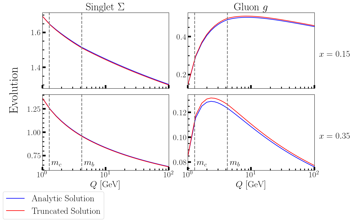
Figure 1: Comparison of the action of the Evolution Operators $\mathbf{E}^{\text{\footnotesize NLO}}$ of Eq. (II.2) (Analytic Solution) and $\overline{\mathbf{E}}^{\text{\footnotesize NLO}}$ of Eq. (33) (Truncated Solution) on the simple proton model described in Eqs. (34). The distributions in $x$-space are defined in Eq. (35). The left panels refer to the flavor-singlet quark distributions $\Sigma=2\,u_{V}+\,d_{V}+6\,q_{\text{\footnotesize sea}}$, while the right panels are dedicated to the gluon distributions $g$. The thresholds at charm and bottom quarks are shown.

III Theoretical uncertainties and Violation of the Evolution Equations

In order to study the violation induced by the approximated solution $\mathbf{E}^{\text{\footnotesize sol}}$, we introduce the Violation Operator:

$$\mathbf{V}^{\text{\footnotesize sol}}\left(N;a_{0},a_{S}(Q)\right)=\frac{\partial\mathbf{E}^{\text{\footnotesize sol}}\left(N;a_{0},a_{S}(Q)\right)}{\partial\log{Q^{2}}}-\left(a_{S}(Q)\mathbf{P}_{0}(N)+a_{S}^{2}(Q)\mathbf{P}_{1}(N)\right)\mathbf{E}^{\text{\footnotesize sol}}\left(N;a_{0},a_{S}(Q)\right).$$ (36)

Similarly to Eq. (35), we define the distributions associated to the violation as:

$$\Delta\mathbf{q}^{\text{\footnotesize sol}}_{S}(x,Q)=\int\frac{dN}{2\pi i}x^{-N}\,\mathbf{V}^{\text{\footnotesize sol}}\left(N;a_{0},a_{S}(Q)\right)\,\mathbf{q}_{S}(x,Q_{0})\quad\text{with: }\Delta\mathbf{q}_{S}=\begin{pmatrix}\Delta\Sigma\\ \Delta g\end{pmatrix}$$ (37)

The more the solution is accurate, the more the violation above is smaller. We can explicitly compute the violations induced by the Analytic Solution of Eq. (II.2) and the Truncated Solution of Eq. (33). They are, respectively:

$$\mathbf{V}^{\text{\footnotesize NLO}}\left(N;a_{0},a_{S}\right)=a_{S}^{2}\beta_{0}e^{h_{1}(a_{0},a_{S})\mathbf{R}_{0}(N)}\Bigg{(}\left[\mathbf{E}_{\text{\footnotesize int}}\left(N;a_{0},a_{S}\right),e^{-h_{1}(a_{0},a_{S})\mathbf{R}_{0}(N)}\left[\mathbf{R}_{1}(N),e^{h_{1}(a_{0},a_{S})\mathbf{R}_{0}(N)}\right]\right]$$

$$\quad-\frac{\sinh{\left(h_{1}(a_{0},a_{S})\Delta_{0}(N)\right)}}{\Delta_{0}(N)}\mathbf{E}_{\text{\footnotesize int}}\left(N;a_{0},a_{S}\right)e^{-h_{4}(\Delta_{0}(N),a_{0},a_{S})}\left[\left[\mathbf{R}_{0}(N),\mathbf{R}_{1}(N)\right],e^{h_{4}(\Delta_{0}(N),a_{0},a_{S})}\right]\Bigg{)}$$ (38a)

$$\overline{\mathbf{V}}^{\text{\footnotesize NLO}}\left(N;a_{0},a_{S}\right)=a_{S}^{3}\beta_{1}\mathbf{R}_{1}(N)e^{h_{1}(a_{0},a_{S})\mathbf{R}_{0}(N)}-a_{S}^{2}\beta_{0}\left(a_{S}\mathbf{U}_{1}(N)\,e^{h_{1}(a_{0},a_{S})\mathbf{R}_{0}(N)}-a_{0}\,e^{h_{1}(a_{0},a_{S})\mathbf{R}_{0}(N)}\mathbf{U}_{1}(N)\right)$$ (38b)

where the operator $\mathbf{E}_{\text{\footnotesize int}}=e^{-h_{1}\,\mathbf{R}_{0}}\mathbf{E}^{\text{\footnotesize NLO}}$ is the product of the last three factors in Eq. (II.2). From these expressions and from the fact that all the functions $h_{i}$ vanishes at the input scale, it follows that $\mathbf{V}^{\text{\footnotesize NLO}}$ is correctly zero in the limit $a_{S}\to a_{0}$, while $\overline{\mathbf{V}}^{\text{\footnotesize NLO}}$ tends to $a_{0}^{3}\beta_{1}\mathbf{R}_{1}$. This is clearly a N³LO violation, hence higher order with respect to the accuracy of the solution. However, it still is a matter of concern, as it spoils the assumption that the Evolution Operator is unity at the input scale.

Figure 2: Comparison of the action of the Violation Operators $\mathbf{V}^{\text{\footnotesize NLO}}$ of Eq. (38) (Analytic Solution) and $\overline{\mathbf{V}}^{\text{\footnotesize NLO}}$ of Eq. (36) (Truncated Solution) on the simple proton model described in Eqs. (34) for $1$ Gev $\geq Q\geq 5000$ GeV. Quark thresholds are indicated by the vertical dashed lines in the upper panel. The violation induced by the Analytic Solution of is systematically smaller than the violation introduced by the truncated solution, by several orders of magnitude at $Q\approx Q_{0}$ and for $x\gtrsim 0.1$. The contribution of the top quark is not considered.

IV Logarithmic Accuracy

The energy dependence of the analytic solutions obtained so far has been parametrized in terms of the strong coupling $a_{S}=\alpha_{S}/(4\pi)$, evaluated at the energy scale and at scale $Q$, where clearly, $a_{S}(Q)\leq a_{S}(Q_{0})$ on the support of Eq. (1). These two values are commonly obtained by integrating numerically the Renormalization Group (RG) evolution for the strong coupling:

$$\frac{d}{d\log{Q^{2}}}a_{S}(Q)=\beta\left(a_{S}(Q)\right),$$ (39)

where the beta function is truncated at the desired order in $a_{S}$. The coefficients of the expansions of $\beta(a_{S})$ are currently known up to $5$ loops [22] but usually only the orders required for the specific analysis are kept. For instance, the $h_{i}$ functions calculated in Eqs. (23) have been obtained truncating the expansion for the $\beta$ function at NLO and hence the solution of Eq. (39) has to be consistently considered at the same perturbative order.

Depending on the purpose of the analysis, it might be worth to solve analytically also the RG evolution for $a_{S}$. The boundary condition is usually chosen to be the most precise experimental measure available [23] for $\alpha_{S}$, taken at the mass $m_{Z}$ of the $Z$ boson. Couplings at different scales are then expressed in terms of $a_{Z}=a_{S}(m_{Z})$. Although an exact solution can only be obtained at LO, it is possible to obtain good approximations of the numeric integrations by using the following expansion:

$$a_{S}(Q)=\frac{a_{Z}}{1-\lambda}\left(1-a_{Z}\frac{\beta_{1}}{\beta_{0}}\frac{\log{(1-\lambda)}}{1-\lambda}-a_{Z}^{2}\frac{\beta_{1}^{2}}{\beta_{0}^{2}}\frac{1}{(1-\lambda)^{2}}\left(\log{(1-\lambda)}-\log^{2}{(1-\lambda)+\left(1-\frac{\beta_{0}\beta_{2}}{\beta_{1}}\right)\lambda}\right)+\dots\right)$$ (40)

where $\lambda=2a_{Z}\beta_{0}\log{(m_{Z}/Q)}$. At the input scale, where the logarithms size is the largest possible and the errors are maximized, the first two terms of this expansion produce a discrepancy about $2\%$ with the numerical solution at NLO, decreasing to about $1\%$ if the first three terms are compared with the NNLO numeric integration.

The approximations introduced to get to Eq. (40) can be iterated to express the coupling at the input scale $a_{0}$ in terms of the coupling $a_{S}(Q)$. This approach would effectively result in an expansion in (inverse) powers of the logarithms $L=\log{(Q/Q_{0})}$ and its accuracy would degrade as the energy $Q$ increases. Substituting it in Eqs. (23), we obtain the following expansions for the functions $h_{i}$:

$$h_{1}(a_{0},a_{S})=f_{1}(\lambda)+\frac{1}{L}f_{2}^{(1)}(\lambda)+\mathcal{O}\left(\frac{1}{L^{2}}\right);$$ (41a)

$$h_{2}(a_{0},a_{S})=\frac{1}{L}f_{2}^{(2)}(\lambda)+\mathcal{O}\left(\frac{1}{L^{2}}\right);$$ (41b)

$$h_{3}(\Delta,a_{0},a_{S})=\frac{1}{L}f_{3}(\Delta,\lambda)+\mathcal{O}\left(\frac{1}{L^{2}}\right);$$ (41c)

$$h_{4}(\Delta,a_{0},a_{S})=\frac{1}{L}f_{4}(\Delta,\lambda)+\mathcal{O}\left(\frac{1}{L^{2}}\right),$$ (41d)

where this time $\lambda=2a_{S}(Q)\beta_{0}L$ and the functions $f_{i}$ are:

$$f_{1}(\lambda)=-\log{(1-\lambda)};$$ (42a)

$$f_{2}^{(1)}(\lambda)=-\frac{1}{2\beta_{0}}\frac{\beta_{1}}{\beta_{0}}\frac{\lambda}{1-\lambda}\log{(1-\lambda)};$$ (42b)

$$f_{2}^{(2)}(\lambda)=\frac{1}{2\beta_{0}}\frac{\lambda^{2}}{1-\lambda};$$ (42c)

$$f_{3}(\Delta,\lambda)=-\frac{1}{4\beta_{0}}\lambda\left(\frac{2}{(1-\Delta^{2})}\frac{1}{1-\lambda}+\frac{1}{\Delta}\left(\frac{(1-\lambda)^{\Delta}}{1+\Delta}-\frac{(1-\lambda)^{-\Delta}}{1-\Delta}\right)\right);$$ (42d)

$$f_{4}(\Delta,\lambda)=-\frac{1}{4\beta_{0}}\frac{\lambda}{1-\lambda}\frac{1}{\Delta^{2}}\left(-\frac{2\left(1-(1-\Delta^{2})\lambda\right)}{1-\Delta^{2}}+\frac{(1-\lambda)^{\Delta}}{1+\Delta}+\frac{(1-\lambda)^{-\Delta}}{1-\Delta}\right).$$ (42e)

The expressions in Eq. (41) can be legitimately regarded as Next-Leading-Log (NLL) accurate. The determination of the next log-order, proportional to $L^{-2}$, would systematically require the use of the QCD beta function at NNLO. The functions $f_{i}$ are singular in $\lambda=1$, which sets the limit where the expansion in powers of logarithms stops to converge.

The application of this strategy to the solution of the DGLAP evolution leads to the NLL expression for the Evolution Operator determined in Eq. (18). In this regard, we can now express it in terms of the original splitting kernels $\mathbf{P}$ instead of the $\mathbf{R}$ operators introduced in Eq. (20). The only contribution that has to be re-arranged is the second matrix exponential in Eq. (18), as its exponent is related to the sum of $\mathbf{P}_{0}$ and $\mathbf{P}_{1}$. However, at NLL it can be equivalently written as:

$$\text{exp}\left(h_{2}(a_{0},a_{S})\mathbf{R}_{1}\right)=\text{exp}\left(\frac{1}{L}f_{2}^{(2)}(\lambda)\left(\frac{1}{\beta_{0}}\mathbf{P}_{1}-\frac{\beta_{1}}{\beta_{0}^{2}}\mathbf{P}_{0}\right)+\mathcal{O}\left(\frac{1}{L^{2}}\right)\right)=$$

$$\quad\text{exp}\left(-\frac{1}{L}\frac{\beta_{1}}{\beta_{0}^{2}}f_{2}^{(2)}(\lambda)\mathbf{P}_{0}\right)\text{exp}\left(\frac{1}{L}f_{2}^{(2)}(\lambda)\frac{1}{\beta_{0}}\mathbf{P}_{1}\right)\,\left(1+\mathcal{O}\left(\frac{1}{L^{2}}\right)\right)$$ (43)

where in the last step we have used the Zassenhaus formula of Eq. (3). The example above shows how easy is to compute the leading contributions at a given log-order, as the size of every term is uniquely and completely fixed. In conclusion, the NLL Evolution Operator reads as:

$$\mathbf{E}^{\text{\footnotesize NLL}}\left(N;Q_{0},Q\right)=\text{exp}\left(\left(\widetilde{f}_{1}(\lambda)+\frac{1}{L}\widetilde{f}_{2}^{\;(1)}(\lambda)\right)\mathbf{P}_{0}(N)\right)\text{exp}\left(\frac{1}{L}\widetilde{f}_{2}^{\;(2)}(\lambda)\mathbf{P}_{1}(N)\right)$$

$$\quad\times\text{exp}\left(\frac{1}{L}\widetilde{f}_{3}\left(\frac{\widetilde{\Delta}_{0}(N)}{\beta_{0}},\lambda\right)\left[\mathbf{P}_{0}(N),\mathbf{P}_{1}(N)\right]\right)\text{exp}\left(\frac{1}{L}\widetilde{f}_{4}\left(\frac{\widetilde{\Delta}_{0}(N)}{\beta_{0}},\lambda\right)\left[\mathbf{P}_{0}(N),\left[\mathbf{P}_{0}(N),\mathbf{P}_{1}(N)\right]\right]\right).$$ (44)

where $\widetilde{\Delta}_{0}$ is the difference of the eigenvalues of $\mathbf{P}_{0}$ and the $\widetilde{f}_{i}$ functions are:

$$\widetilde{f}_{1}(\lambda)=\frac{1}{\beta_{0}}f_{1}(\lambda);$$ (45a)

$$\widetilde{f}_{2}^{\;(1)}(\lambda)=\frac{1}{\beta_{0}}\left(f_{2}^{\;(1)}(\lambda)-b_{1}f_{2}^{\;(2)}(\lambda)\right);$$ (45b)

$$\widetilde{f}_{2}^{\;(2)}(\lambda)=\frac{1}{\beta_{0}}f_{2}^{\;(2)}(\lambda);$$ (45c)

$$\widetilde{f}_{3}(\Delta,\lambda)=\frac{1}{\beta_{0}^{2}}f_{3}(\Delta,\lambda);$$ (45d)

$$\widetilde{f}_{4}(\Delta,\lambda)=\frac{1}{\beta_{0}^{3}}f_{4}(\Delta,\lambda).$$ (45e)

Notice that the functions $\widetilde{f}_{1}$ and $\widetilde{f}_{2}$ precisely correspond to the NLL approximation of the integrals $\int_{Q_{0}}^{Q}d(\log{\mu^{2}})a_{S}(\mu)$ and $\int_{Q_{0}}^{Q}d(\log{\mu^{2}})a^{2}_{S}(\mu)$, respectively.

The solution presented in Eq. (IV) is remarkable for many aspects. First of all, while it is possible to give different interpretations of the label “NLO” and produce different analytic expressions as testified by Eqs. (II.2) and (33), the meaning of NLL is unambiguous and it specifically refers to a result in which all the relevant logarithms are exponentiated and organized in descending powers. Such expressions are often at the core of many observables and suited for a wide range of applications, from event-shape observables to transverse momentum dependent cross sections [24, 25, 26, 27, 28], where the relevant log-orders are usually obtained withing the framework of resummation. In particular, parton distributions are used as inputs in Transverse Momentum Dependent (TMD) densities, where it is common practice to take into account the log-ordering in terms of logarithms of transverse distance [29, 30, 31]. Although it is beyond the purpose of this paper to discuss about the correct implementation of the log counting within the TMD factorization and there is a dedicated recent literature on this subject [32, 33], the solution obtained in Eq. (IV) would be particularly suited for applications in the TMD case and for simultaneous extractions of collinear parton densities together with their TMD counterparts. More generally, studying the effects of the collinear functions in TMD observables is triggering the interest of the TMD community [32, 33, 34, 35] and most modern analyses are also devoted to this topic.

Notice that also the truncated solution of Eq. (33) can be expanded in powers of $L$, but such logarithms would not be exponentiated and the resulting approximation would not properly resum all the NLL contributions to the parton distributions. Therefore, Eq. (IV) is the only NLL accurate result for the singlet sector of the DGLAP evolution. Moreover, it is completely based on a analytic approach: every ingredient in $\mathbf{E}^{\text{\footnotesize NLL}}$ has been explicitly computed analytically. Finally, we stress once again that the expansion in powers of $1/L$ is extremely transparent and all the neglected terms are assigned with a well defined scaling. As a consequence, the Violation Operator of Eq. (36) associated to the NLL solution is certainly of order $1/L^{2}$, as well as the effect of the perturbative hysteresis [13].

Despite its appealing features, the solution in Eq. (IV) also has disadvantages. In particular, being an approximation of the (already approximated) NLO result of Eq. (18), it is less precise when compared with the exact numerical solution of the DGLAP evolution. Therefore, given the differential equation of Eq. (2), the choice of which solution to adopt among the three in Eqs. (II.2), (33) and  (IV) ultimately depends on the problem at hand. A comprehensive comparison for all the analytic solutions discussed in this work is shown in Fig. 3.

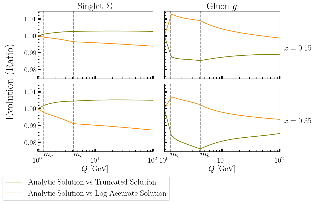
Figure 3: Comparison of the action of the Evolution Operators $\mathbf{E}^{\text{\footnotesize NLO}}$ of Eq. (II.2) (Analytic Solution), $\overline{\mathbf{E}}^{\text{\footnotesize NLO}}$ of Eq. (33) (Truncated Solution) and $\mathbf{E}^{\text{\footnotesize NLL}}$ (Log-Accurate Solution) on the simple proton model described in Eqs. (34). The lines refer to ratios of distributions in $x$-space defined in Eq. (35). Green lines compare the Analytic Solution and the Truncated Solution, while the orange lines compare the Analytic Solution and the Log-Accurate Solution. The left panels refer to the flavor-singlet quark distributions $\Sigma=2\,u_{V}+\,d_{V}+6\,q_{\text{\footnotesize sea}}$, while the right panels are dedicated to the gluon distributions $g$. The thresholds at charm and bottom quarks are shown.

V Conclusions

The DGLAP evolution is at the core of the research on strong interactions, as it is used to predict the energy dependence of the Parton Distribution Functions, which are key tools for studying hadronic processes. Providing accurate solutions is thus a necessary task for keeping up with the increasing precision of modern experiments. Together with the solutions obtained from a strict numeric integration of Eq. (1), analytic approaches are also worth to be investigated. Explicit analytic expressions not only offer a clearer point of view on the effect of the evolution, but they also provide a cleaner determination of the theoretical uncertainties. Such arguments are particularly relevant in the singlet sector, where a closed analytic form cannot be obtained and hence one has necessarily to rely on some approximation.

In this work, three different analytic solutions at NLO have been addressed and compared with each other. The proper mathematical formalism for treating the evolution in 2 dimensions has been introduced and it has been used to obtain a novel result, devised to be as close as possible to the exact numerical solution and, at the same time, to preserve the expected mathematical features (such as the exponentiation) of the result of Eq. (2). This Analytic Solution has been presented in Eq. (II.2) and shown to be systematically more precise than the popular Truncated Solution of Eq. (33) and widely used in phenomenological analyses based on analytic approaches. On the other hand, it has a more complicated structure involving four matrix exponentials and non-trivial functions. It is remarkable, though, that despite such complications it only requires to diagonalize three matrices, related to the splitting kernels up to NLO and their commutator. Finally, we have also presented in Eq. (IV) the Log-Accurate Solution at NLL. Being obtained as a further approximation, it is less accurate than the NLO solutions. However, it provides a cleaner estimate of the theoretical uncertainties. In fact, all the neglected terms, as well as the size of the violation of the original differential equation, scale as $1/L^{2}$. Ultimately, it is the purpose of the analysis in which the DGLAP evolution is employed to determine which is the best result to choose. If the goal is precision (and mathematical elegance) than the Analytic Solution of Eq. (II.2) might be the best option. If instead the Parton Distributions are supposed to be implemented in some resummation formalism, by extension including the TMD case, or whenever a better control on the size of the theoretical errors has been given priority, then the Log-Accurate Solution of Eq. (IV) could be the expression to adopt. Finally, if simplicity is the key word, as for fast code implementations, then the usual Truncated Solution of Eq. (33) is to be preferred.

In conclusion, a comprehensive overview of different analytic approaches to the Singlet DGLAP evolution has been presented and novel analytic results have been explicitly computed, considering associated advantages and disadvantages. This sets the ground for enriching the existing codes based on analytic solutions of DGLAP equations and thus for developing new and more refined tools in light of a promising phenomenology in the context of Parton Distributions and hadronic processes.

Appendix A Results for matrix representations in two dimensions

In this Section, we collect some useful results holding in $2$-dimensions. We introduce the following notation for the nested $n$-commutator of the matrix $\mathbf{A}$ with the matrix $\mathbf{B}$:

$$\left[\left(\mathbf{A}\right)^{n},\mathbf{B}\right]=\left[\mathbf{A},\left[\mathbf{A\big{[}\dots},\mathbf{B}\right],\dots\big{]}\right],$$ (46)

where the matrix $\mathbf{A}$ appears $n$ times. The main simplifications occurring in $2$ dimensions are consequences of the following Lemma:

Lemma 1.

Let $\mathbf{A}$ and $\mathbf{B}$ be $2$ dimensional diagonalizable matrices and let $K(\mathbf{A})=\text{Tr}(\mathbf{A})^{2}-4\text{Det}(\mathbf{A})$. If the commutator $\left[\mathbf{A},\mathbf{B}\right]$ is diagonalizable, then every $n$-commutator of $\mathbf{A}$ with $\mathbf{B}$ is proportional either to $\left[\mathbf{A},\mathbf{B}\right]$ or to $\left[\mathbf{A},\left[\mathbf{A},\mathbf{B}\right]\right]$, depending on the parity of the occurrencies of $\mathbf{A}$:

$$\left[\left(\mathbf{A}\right)^{2n+1},\mathbf{B}\right]=K(\mathbf{A})^{n}\left[\mathbf{A},\mathbf{B}\right],\quad n\geq 0$$ (47a)

$$\left[\left(\mathbf{A}\right)^{2n+2},\mathbf{B}\right]=K(\mathbf{A})^{n}\left[\mathbf{A},\left[\mathbf{A},\mathbf{B}\right]\right],\quad n\geq 0$$ (47b)

Proof.

First, we prove that every $(2n+1)$-commutator is similar to a diagonal matrix, while every $(2n+2)$-commutator is similar to a anti-diagonal matrix, for $n\geq 0$. Since the commutator $\left[\mathbf{A},\mathbf{B}\right]$ is diagonalizable, it exists a matrix $\mathbf{V}_{C}$ such that $\mathbf{D}_{1}=\mathbf{V}_{C}^{-1}\left[\mathbf{A},\mathbf{B}\right]\mathbf{V}_{C}$. The same similarity transformation applied to the $2$-commutator gives $\mathbf{V}_{C}^{-1}\left[\left(\mathbf{A}\right)^{2},\mathbf{B}\right]\mathbf{V}_{C}=\left[\mathbf{V}_{C}^{-1}\mathbf{A}\mathbf{V}_{C},\mathbf{D}_{1}\right]=\widetilde{\mathbf{D}}_{2}$, which is certainly antidiagonal in two dimensions. Analogously, the $3$-commutators maps to $\mathbf{V}_{C}^{-1}\left[\left(\mathbf{A}\right)^{3},\mathbf{B}\right]\mathbf{V}_{C}=\left[\mathbf{V}_{C}^{-1}\mathbf{A}\mathbf{V}_{C},\widetilde{\mathbf{D}}_{2}\right]=\mathbf{D}_{3}$, which is certainly diagonal in two dimensions. Proceeding by induction, it readily follows that for $n\geq 0$:

$$\mathbf{D}_{2n+1}=\mathbf{V}_{C}^{-1}\left[\left(\mathbf{A}\right)^{2n+1},\mathbf{B}\right]\mathbf{V}_{C}$$ (48a)

$$\widetilde{\mathbf{D}}_{2n+2}=\mathbf{V}_{C}^{-1}\left[\left(\mathbf{A}\right)^{2n+2},\mathbf{B}\right]\mathbf{V}_{C}$$ (48b)

where odd and even labels corresponds to diagonal and anti-diagonal matrices, respectively.

The second part of the proof is based on the observation that, in two dimensions, the matrix $\mathbf{A}^{\prime}=V_{C}^{-1}\mathbf{A}V_{C}$ has equal elements on its diagonal. It can be generically written as:

$$\mathbf{A}^{\prime}=\begin{pmatrix}a&&b\\ c&&a\end{pmatrix}.$$ (49)

Thus, if the commutator $\left[\mathbf{A},\mathbf{B}\right]$ has eigenvalues $\pm d_{1}$, the anti-diagonal matrix $\widetilde{\mathbf{D}}_{2}$ is given by:

$$\widetilde{\mathbf{D}}_{2}=\left[\mathbf{A}^{\prime},\mathbf{D}_{1}\right]=2d_{1}\begin{pmatrix}0&&-b\\ c&&0\end{pmatrix}.$$ (50)

Iterating this procedure and proceeding by induction, it follows that for $n\geq 0$:

$$\mathbf{D}_{2n+1}=(4bc)^{n}\mathbf{D}_{1}$$ (51a)

$$\widetilde{\mathbf{D}}_{2n+2}=(4bc)^{n}\widetilde{\mathbf{D}}_{2}$$ (51b)

Since $4bc=K(\mathbf{A}^{\prime})=K(\mathbf{A})$, this completes the proof. ∎

We can now easily obtain the following fundamental results for two dimensional matrix representations:

Lemma 2 (Hadamard’s Lemma).

Let $\mathbf{A}$ and $\mathbf{B}$ be $2\times 2$ matrices. Then, the Hadamard’s Lemma reads as:

$$e^{\mathbf{A}}\mathbf{B}e^{-\mathbf{A}}=\mathbf{B}+\frac{\sinh{\left(\Delta_{A}\right)}}{\Delta_{A}}\left[\mathbf{A},\mathbf{B}\right]+\frac{\cosh{\Delta_{A}}-1}{\Delta_{A}^{2}}\left[\mathbf{A},\left[\mathbf{A},\mathbf{B}\right]\right],$$ (52)

where $\Delta_{A}=\sqrt{K(\mathbf{A})}$ is the difference of the eigenvalues of $A$ and $K(\mathbf{A})$ is the invariant introduced in Lemma 1. As a corollary, it follows that:

$$e^{\mathbf{A}}e^{\mathbf{B}}=e^{\mathbf{B}+\frac{\sinh{\left(\Delta_{A}\right)}}{\Delta_{A}}\left[\mathbf{A},\mathbf{B}\right]+\frac{\cosh{\Delta_{A}}-1}{\Delta_{A}^{2}}\left[\mathbf{A},\left[\mathbf{A},\mathbf{B}\right]\right]}e^{\mathbf{A}},$$ (53)

Lemma 3.

[Zassenhaus formula] Let $\mathbf{A}$ and $\mathbf{B}$ be $2\times 2$ matrices. Then, the exponential of their sum is:

$$e^{t\left(\mathbf{A}+\mathbf{B}\right)}=e^{t\mathbf{A}}e^{t\mathbf{B}}\,\mathcal{T}\text{exp}\Bigg{(}\int_{0}^{t}ds\,\Big{\{}-\frac{\sinh{\left(s\Delta_{A}\right)}}{\Delta_{A}}\left(\left[\mathbf{A},\mathbf{B}\right]+\frac{\sinh{\left(s\Delta_{B}\right)}}{\Delta_{B}}\left[\mathbf{A},\left(\mathbf{B}\right)^{2}\right]-\frac{\cosh{\left(s\Delta_{B}\right)}-1}{\Delta_{B}^{2}}\left[\mathbf{A},(\mathbf{B})^{3}\right]\right)$$

$$\qquad+\frac{\cosh{\left(s\Delta_{A}\right)}-1}{\Delta_{A}^{2}}\left(\left[\left(\mathbf{A}\right)^{2},\mathbf{B}\right]+\frac{\sinh{\left(s\Delta_{B}\right)}}{\Delta_{B}}\left[\left(\mathbf{A}\right)^{2},\left(\mathbf{B}\right)^{2}\right]-\frac{\cosh{\left(s\Delta_{B}\right)}-1}{\Delta_{B}^{2}}\left[\left(\mathbf{A}\right)^{2},\left(\mathbf{B}\right)^{3}\right]\right)\Big{\}}\Bigg{)}$$ (54)

where $\mathcal{T}$ represents the Dyson time-ordering [19] and $\Delta_{A}$ and $\Delta_{B}$ are the differences of the eigenvalues of the matrices $\mathbf{A}$ and $\mathbf{B}$, respectively.

Proof.

The proof follows from the integral representation of the Zassenhaus formula [36] and from the iterated application of Lemma 1. ∎