On the self-similarity of unbounded viscous Marangoni flows

Abstract

The Marangoni flow induced by an insoluble surfactant on a fluid-fluid interface is a fundamental problem investigated extensively due to its implications in colloid science, biology, the environment, and industrial applications. Here, we study the limit of a deep liquid subphase with negligible inertia (low Reynolds number $Re\ll{1}$), where the two-dimensional problem has been shown to be described by the complex Burgers equation. We analyze the problem through a self-similar formulation, providing further insights into its structure and revealing its universal features. Six different similarity solutions are found. One of the solutions includes surfactant diffusion, whereas the other five, which are identified through a phase-plane formalism, hold only in the limit of negligible diffusion (high surface Péclet number $Pe_{s}\gg{1}$). Surfactant ‘pulses’, with a locally higher concentration that spreads outward, lead to two similarity solutions of the first kind with a similarity exponent $\beta=1/2$. On the other hand, distributions that are locally depleted and flow inwards lead to similarity of the second kind, with two different exponents that we obtain exactly using stability arguments. We distinguish between ‘dimple’ solutions, where the surfactant has a quadratic minimum and $\beta=2$, from ‘hole’ solutions, where the concentration profile is flatter than quadratic and $\beta=3/2$. Each of these two cases exhibits two similarity solutions, one prior to a critical time $t_{*}$ when the derivative of the concentration is singular, and another one valid after $t_{*}$. We obtain all six solutions in closed form, and discuss useful predictions that can be extracted from these results.

1 Introduction

When the interface between two fluids is laden with a non-uniform distribution of surfactant, the resulting imbalance of surface tension triggers a Marangoni flow (Scriven & Sternling, 1960; de0Gennes et0al., 2004). The underlying dynamics are nonlinear, since the surfactant distribution, which sets the surface-driven fluid flow, is itself redistributed by the resulting velocity field through advection. This two-way coupled problem has been the focus of numerous studies, as surface-active molecules are virtually unavoidable in realistic multiphase flow problems appearing both in natural and engineered systems (Manikantan & Squires, 2020). For example, ambient amounts of surfactant are known to critically alter flows relevant to the environment like the motion of bubbles and drops, through a mechanism first proposed by Frumkin & Levich (1947) that has since been studied extensively (Schechter & Farley, 1963; Wasserman & Slattery, 1969; Sadhal & Johnson, 1983; Griffith, 1962; Cuenot et0al., 1997; Wang et0al., 1999; Palaparthi et0al., 2006, to name a few). Likewise, the surface of the ocean is affected by surfactants, which alter the dynamics of waves ranging from small capillary ripples (Lucassen & Van Den0Tempel, 1972; Alpers & Hühnerfuss, 1989) to larger spilling and plunging breakers (Liu & Duncan, 2003; Erinin et0al., 2023). Marangoni flows also play an important role in biological fluid mechanics, both in physiological transport processes within the lung (Grotberg et0al., 1995) or the ocular globe (Zhong et0al., 2019), and in the motion of colonies of microorganisms that generate biosurfactants (Botte & Mansutti, 2005; Trinschek et0al., 2018). In industrially relevant applications, it is well-known that surface-active molecules influence the dip coating of plates and fibers (Park, 1991; Quéré, 1999), the drag reduction of superhydrophobic surfaces (Peaudecerf et0al., 2017; Song et0al., 2018; Temprano-Coleto et0al., 2023), or the stability of foams (Breward & Howell, 2002; Cantat et0al., 2013).

One the most fundamentally important examples of flows induced by surfactants is the so-called ‘Marangoni spreading’ (Matar & Craster, 2009), where a locally concentrated surfactant spreads unopposed on a clean interface until it reaches a uniform equilibrium concentration. Early quantitative studies examined surfactant spreading on thin films, due to their relevance in pulmonary flows (Ahmad & Hansen, 1972; Borgas & Grotberg, 1988; Gaver & Grotberg, 1990, 1992). The pioneering work of Jensen & Grotberg (1992) investigated the spreading of insoluble surfactant from the perspective of self-similarity, a powerful theoretical tool to identify universal, scale-free behavior in physical systems (Barenblatt, 1996). Several studies of Marangoni flows on thin films based on self-similarity have since followed. For example, Jensen & Grotberg (1993) described the spreading of a soluble surfactant, while Jensen (1994) re-examined the insoluble case, finding additional self-similar solutions for distributions that are not locally concentrated, but depleted of surfactant, which ‘fill’ under the action of Marangoni stresses. Self-similarity was also examined for a deep fluid subphase by Jensen (1995), considering the limit of dominant fluid inertia (i.e. at high Reynolds number).

In all the above studies, the problem is simplified by the existence of a confining lengthscale in the fluid subphase, either the thickness of the thin liquid film or the width of the momentum boundary layer. Thess et0al. (1995) considered the case of a deep fluid subphase at low Reynolds number, where the fluid flow is unconfined, and identified that the resulting problem is nonlocal, with the velocity field at any given position depending on the surfactant distribution on the whole interface. Theoretical work in this limit followed (Thess, 1996; Thess et0al., 1997), but analytical progress proved challenging due to the nonlocal nature of the problem. Recently, Crowdy (2021b) showed that this problem is equivalent to Burgers equation, effectively providing a local reformulation using complex variables. This key insight has allowed for the formulation of some exact solutions (Crowdy, 2021b; Bickel & Detcheverry, 2022), also facilitating the study of extensions of the problem (Crowdy, 2021a; Crowdy et0al., 2023).

Even after this simplification of low-Reynolds-number, deep-subphase Marangoni flow, exact solutions to the Burgers equation can be written explicitly only for a selected subset of initial conditions, limiting the generality of the resulting physical insights. In this paper, we analyze the problem from the perspective of self-similarity, which has provided key physical insights not only to Marangoni spreading, but to many other problems like boundary layer theory (Leal, 2007), liquid film spreading (Huppert, 1982; Brenner & Bertozzi, 1993), drop coalescence (Kaneelil et0al., 2022), and capillary pinching (Eggers, 1993; Brenner et0al., 1996; Day et0al., 1998). We show that self-similarity not only reveals new universal features about the problem that are independent of the specific boundary conditions, but also gives rise to a beautiful mathematical structure with six different similarity solutions and three different rational exponents, all of which can be obtained in closed form.

We present the general formulation of the problem in section 2. Section 3 analyzes the case of advection-dominated Marangoni flows, i.e. in the limit of infinite surface Péclet number $Pe_{s}^{-1}=0$. In particular, the different possible similarity solutions for this limit are identified through a combination of a phase-plane formalism (section 3.1) and stability analysis (section LABEL:sec:stability). In section LABEL:sec:spreading_sols, we consider the case of ‘spreading’, where locally concentrated surfactant induces an outward flow, and derive one solution without diffusion (section LABEL:sec:spreading_sols_no_diff) and one with diffusion (section 4.2). Section 5 analyzes locally depleted surfactant distributions, which induce a ‘filling’ flow inwards. Depending on the initial conditions of the problem, we distinguish that the filling dynamics converge to either ‘dimple’ (section 5.1) or ‘hole’ (section 5.2) solutions. For either case, we derive one similarity solution that holds prior to a reference time $t_{*}$ where the solution has a singularity, and another similarity solution valid after $t_{*}$. We discuss these results and draw conclusions in section 6.

2 Problem formulation

We consider the dynamics of an insoluble surfactant evolving on the free surface of a layer of incompressible, Newtonian fluid of density $\rho$ and dynamic viscosity $\mu$. Our focus is the limit of small Reynolds ($Re$) and capillary ($Ca$) numbers given by

$$Re=\dfrac{\rho{u_{c}}{l_{c}}}{\mu}\ll{1},\qquad\qquad Ca=\dfrac{\mu{u_{c}}}{\gamma_{0}}\ll{1},$$ (1)

where $\gamma_{0}$ is the surface tension of the clean (surfactant-free) interface, and $l_{c}$ and $u_{c}$ are the characteristic length and velocity scales of the problem, respectively. In this asymptotic limit, surface tension dominates over viscous stresses, keeping the interface flat. In addition, fluid inertia is negligible and the velocity field $\bm{u}(\bm{x},t)$, which depends on both time $t$ and position $\bm{x}$, is well described by the continuity and Stokes equations

$$\bm{\nabla}\bm{\cdot}\bm{u}=0,\qquad\qquad\bm{\nabla}\bm{\cdot}\mathsfbi{T}={\bf 0},$$ (2)

where $\mathsfbi{T}$ is the second-order stress tensor, $\mathsfbi{T}=-p\,\mathsfbi{I}+\mu\left[\bm{\nabla}\bm{u}+{\left(\bm{\nabla}\bm{u}\right)}^{\mathsf{T}}\right]$, $p$ the mechanical pressure, and $\mathsfbi{I}$ the identity tensor.

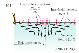
(a)

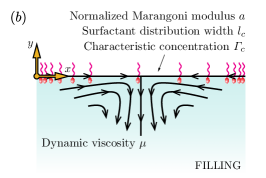
(b)

Figure 1: A non-homogeneous distribution of insoluble surfactant, with concentration $\Gamma(x,t)$, induces a velocity field $\bm{u}(\bm{x},t)$ within its fluid subphase through interfacial Marangoni stresses. The surfactant is itself advected by the resulting interfacial velocity $u_{s}(x,t)=\left.\bm{u}\bm{\cdot}\bm{e}_{x}\right|_{y=0}$, leading to a two-way coupled problem. $(a)$ For a localized pulse of surfactant, the Marangoni flow results in outward ‘spreading’. $(b)$ When the surfactant distribution is instead depleted at its center (a hole or a dimple), the result is an inward ‘filling’ flow. All the dimensional parameters of the model considered here are highlighted in panel $(b)$.

For sufficiently elongated surfactant distributions (e.g., a ‘strip’ of surfactant) and a sufficiently deep fluid subphase, the problem can be reduced to the unbounded, two-dimensional scenario displayed in figure 1. We use a coordinate system where $x$ spans the interface and $y$ points away from the fluid subphase, with $\bm{e}_{x}$ and $\bm{e}_{y}$ the unit vectors in the $x$ and $y$ directions. Velocity components are denoted $u$ and $v$, with $\bm{u}=u\bm{e}_{x}+v\bm{e}_{y}$. The domain is considered to be semi-infinite, defined in $x\in(-\infty,\infty)$ and $y\in(-\infty,0\,]$, and the time evolution of the surfactant concentration $\Gamma(x,t)$ is given by

$$\dfrac{\partial\Gamma}{\partial t}+\dfrac{\partial(u_{s}\Gamma)}{\partial x}=D_{s}\dfrac{\partial^{2}\Gamma}{\partial x^{2}},$$ (3)

where $D_{s}$ is the surface diffusivity of the surfactant and $u_{s}=\left.\bm{u}\bm{\cdot}\bm{e}_{x}\right|_{y=0}$ is the interfacial velocity. The boundary conditions at the interface

$$\left[\bm{e}_{y}\bm{\cdot}\mathsfbi{T}\bm{\cdot}\bm{e}_{x}\right]_{y=0} =a\dfrac{\partial\Gamma}{\partial x},$$ (4a)

$$v(y=0) =0,$$ (4b)

are the Marangoni condition (4a) linking viscous stresses to the gradient of surfactant, and the no-penetration kinematic condition (4b). Here, the parameter

$$a=\dfrac{\,\mathrm{d}\gamma}{\,\mathrm{d}\Gamma}$$ (5)

is a normalized Marangoni modulus, indicating the variation of surface tension $\gamma$ with respect to surfactant concentration. We take $D_{s}$ and $a$ to be constants, although they are in general dependent on $\Gamma$ through equations of state $D_{s}(\Gamma)$ and $\gamma(\Gamma)$, e.g., see Manikantan & Squires (2020).

The governing equations (2)-(3) and boundary conditions (4) are supplemented with an initial condition for the surfactant distribution

$$\Gamma(x,t=0)=\Gamma_{0}(x).$$ (6)

The profile $\Gamma_{0}(x)$ introduces the characteristic scale $\Gamma_{c}$, which we will take as the maximum concentration $\Gamma_{c}=\max_{x}{[\Gamma_{0}(x)]}$. Furthermore, the typical width of $\Gamma_{0}(x)$ also sets the lengthscale $l_{c}$ of the problem.

From these constants, dimensional analysis of the Marangoni boundary condition (4a) leads to a natural scale for the velocity magnitude

$$\left[\bm{e}_{y}\bm{\cdot}\mathsfbi{T}\bm{\cdot}\bm{e}_{x}\right]_{y=0}=\left.\mu\dfrac{\partial u}{\partial y}\right|_{y=0}=a\dfrac{\partial\Gamma}{\partial x}\implies u_{c}\approx\dfrac{a\Gamma_{c}}{\mu}.$$ (7)

For the assumptions of $Re\ll{1}$ and $Ca\ll{1}$ to hold, the characteristic concentration $\Gamma_{c}$ and width $l_{c}$ of the surfactant distribution must both be sufficiently small to ensure that

$$l_{c}\Gamma_{c}\ll\dfrac{\mu^{2}}{\rho{a}},\qquad\qquad\Gamma_{c}\ll\dfrac{\gamma_{0}}{a},$$ (8)

providing practical estimates to determine if, for a given set of physicochemical properties $\mu$, $\rho$, $a$, and $\gamma_{0}$, a known surfactant distribution will lead to Marangoni flow in the limit considered in this study.

The full problem, as defined by (2)-(4) and (6), is nonlinear and involves the two-dimensional vector field $\bm{u}$. Thess et0al. (1995) recognized that it was possible to obtain a one-dimensional formulation, using the Fourier transform of (2) to obtain $u_{s}$ as a function of $\Gamma$. Here, we show that the same simplification can be achieved through the boundary integral representation of Stokes flow. Indeed, the velocity field given by (2) at any position $\bm{x}$ along the interface (see Pozrikidis, 1992) can be expressed as

$$\bm{u}(\bm{x},t)=\dfrac{1}{2\pi}\left[\int_{\mathcal{I}}\bm{n}\bm{\cdot}\mathsfbi{K}(\bm{x}-\bm{x}^{\prime})\bm{\cdot}\bm{u}(\bm{x}^{\prime},t)\,\mathrm{d}{S_{\bm{x}^{\prime}}}-\,\,\mathchoice{{\vbox{\hbox{$\textstyle-$ }}\kern-7.83337pt}}{{\vbox{\hbox{$\scriptstyle-$ }}\kern-5.90005pt}}{{\vbox{\hbox{$\scriptscriptstyle-$ }}\kern-4.75003pt}}{{\vbox{\hbox{$\scriptscriptstyle-$ }}\kern-4.25003pt}}\!\int_{\mathcal{I}}\bm{n}\bm{\cdot}\mathsfbi{T}(\bm{x}^{\prime},t)\bm{\cdot}\mathsfbi{J}(\bm{x}-\bm{x}^{\prime})\,\mathrm{d}{S_{\bm{x}^{\prime}}}\right],$$ (9)

where the dash denotes the Cauchy principal value of the integral, $\mathcal{I}$ indicates integration along the interface, $\bm{n}$ is the unit outward normal vector, and the tensors in the integrands are defined as

$$\mathsfbi{J}(\bm{x}) =-\dfrac{1}{\mu}\left(\ln|\bm{x}|\,\mathsfbi{I}-\dfrac{\bm{x}\bm{x}}{|\bm{x}|^{2}}\right),$$ (10a)

$$\mathsfbi{K}(\bm{x}) =-4\,\dfrac{\bm{x}\bm{x}\bm{x}}{|\bm{x}|^{4}}.$$ (10b)

Since the interface remains flat, the outward normal vector simplifies as $\bm{n}=\bm{e}_{y}$, while $\bm{x}$ and $\bm{x}^{\prime}$ are co-linear and parallel to $\bm{e}_{x}$. Therefore, we have $\bm{n}\bm{\cdot}(\bm{x}-\bm{x}^{\prime})=0$ since the vectors are orthogonal, and

$$\bm{n}\bm{\cdot}\mathsfbi{K}(\bm{x}-\bm{x}^{\prime})=-\dfrac{1}{\pi}\,\bm{n}\bm{\cdot}\dfrac{(\bm{x}-\bm{x}^{\prime})(\bm{x}-\bm{x}^{\prime})(\bm{x}-\bm{x}^{\prime})}{|\bm{x}-\bm{x}^{\prime}|^{4}}=\mathsfbi{0},$$ (11)

eliminating the first integral (the ‘single-layer potential’) in equation (9). Taking $(\bm{x}-\bm{x}^{\prime})=(x-x^{\prime})\bm{e}_{x}$ and noting the integrals along the interface are simply along $x^{\prime}$, the interfacial velocity can then be expressed as

$$u_{s}(x,t)=\left.\bm{u}\bm{\cdot}\bm{e}_{x}\right|_{y=0}=\dfrac{1}{2\pi\mu}\,\,\mathchoice{{\vbox{\hbox{$\textstyle-$ }}\kern-7.83337pt}}{{\vbox{\hbox{$\scriptstyle-$ }}\kern-5.90005pt}}{{\vbox{\hbox{$\scriptscriptstyle-$ }}\kern-4.75003pt}}{{\vbox{\hbox{$\scriptscriptstyle-$ }}\kern-4.25003pt}}\!\int_{-\infty}^{\infty}\left[\bm{e}_{y}\bm{\cdot}\mathsfbi{T}(x^{\prime},t)\bm{\cdot}\bm{e}_{x}\right]_{y=0}\Bigl{(}\ln|x-x^{\prime}|-1\Bigr{)}\,\mathrm{d}{x^{\prime}},$$ (12)

which, upon substitution of the Marangoni boundary condition (4a) and integration by parts, becomes

$$u_{s}(x,t)=\dfrac{a}{2\pi\mu} \left\{\Bigl{[}\bigl{(}1+\ln|x-x^{\prime}|\bigr{)}\,\Gamma(x^{\prime},t)\Bigr{]}_{x^{\prime}\to-\infty}^{x^{\prime}\to\infty}+\,\,\mathchoice{{\vbox{\hbox{$\textstyle-$ }}\kern-7.83337pt}}{{\vbox{\hbox{$\scriptstyle-$ }}\kern-5.90005pt}}{{\vbox{\hbox{$\scriptscriptstyle-$ }}\kern-4.75003pt}}{{\vbox{\hbox{$\scriptscriptstyle-$ }}\kern-4.25003pt}}\!\int_{-\infty}^{\infty}\dfrac{\Gamma(x^{\prime},t)}{x-x^{\prime}}\,\mathrm{d}{x^{\prime}}\right\}.$$ (13)

We consider that the far-field values of $\Gamma$ are finite and equal, i.e., $\lim_{x\to\infty}\Gamma(x,t)=\lim_{x\to-\infty}\Gamma(x,t)<\infty$, and therefore the first term in the right-hand side of (13) vanishes. We note that it is not necessary for $\Gamma(x,t)$ to decay as $|x|\to\infty$, a finite far-field value of $\Gamma(x,t)$ is sufficient given that the integrals are understood in a principal value sense. The above leads to the closure relationship

$$u_{s}(x,t)=\dfrac{a}{2\pi\mu}\,\,\mathchoice{{\vbox{\hbox{$\textstyle-$ }}\kern-7.83337pt}}{{\vbox{\hbox{$\scriptstyle-$ }}\kern-5.90005pt}}{{\vbox{\hbox{$\scriptscriptstyle-$ }}\kern-4.75003pt}}{{\vbox{\hbox{$\scriptscriptstyle-$ }}\kern-4.25003pt}}\!\int_{-\infty}^{\infty}\dfrac{\Gamma(x^{\prime},t)}{x-x^{\prime}}\,\mathrm{d}{x^{\prime}}=\dfrac{a}{2\mu}\mathcal{H}[\Gamma],$$ (14)

first derived by Thess et0al. (1995), where the operator $\mathcal{H}\left[\,\,\,\right]$ denotes the Hilbert transform of a function (for details, see King, 2009a, b). This closure relationship results in a one-dimensional problem, only requiring the solution of (3) alongside condition (14). The resulting formulation is, however, nonlocal, as the interfacial velocity $u_{s}$ at any given point depends upon the distribution of $\Gamma$ along the whole real line.

We proceed to nondimensionalize equations (3), (14), and the initial condition (6) using the scales of the problem discussed above. To that end, we apply the rescalings

$$x\to l_{c}{x},\qquad t\to\left(\dfrac{2\mu{l_{c}}}{a\Gamma_{c}}\right)t,\qquad u\to\left(\dfrac{a\Gamma_{c}}{2\mu}\right)u,\qquad\Gamma\to\Gamma_{c}\Gamma,\qquad\Gamma_{0}\to\Gamma_{c}\Gamma_{0},$$ (15)

which leads to a dimensionless problem given by

$$\dfrac{\partial\Gamma}{\partial t}+\dfrac{\partial(\mathcal{H}\left[\Gamma\right]\Gamma)}{\partial x} =\dfrac{1}{Pe_{s}}\dfrac{\partial^{2}\Gamma}{\partial x^{2}},$$ (16a)

$$\Gamma(x,t=0) =\Gamma_{0}(x),$$ (16b)

and where the surface Péclet number is defined as

$$Pe_{s}\vcentcolon=\dfrac{a\Gamma_{c}l_{c}}{2\mu{D_{s}}}.$$ (17)

A major simplification of (16) was introduced recently by Crowdy (2021b) who, through a complex-variable formulation of two-dimensional Stokes flow, showed how a complex dependent variable $\psi=u_{s}-\mathrm{i}\Gamma=\mathcal{H}\left[\Gamma\right]-\mathrm{i}\Gamma$ satisfies

$$\dfrac{\partial\psi}{\partial t}+\psi\dfrac{\partial\psi}{\partial x} =\dfrac{1}{Pe_{s}}\dfrac{\partial^{2}\psi}{\partial x^{2}},$$ (18a)

$$\psi(x,t=0) =\psi_{0}(x)=\mathcal{H}\left[\Gamma_{0}(x)\right]-\mathrm{i}\Gamma_{0}(x),$$ (18b)

where $\psi(x+\mathrm{i}{y},t)$ must be an upper-analytic complex function. This reduction can be realized also by subtracting (16a) from its Hilbert transform, and then recognizing that $\mathcal{H}\left[\partial_{x}\Gamma\right]=\partial_{x}\mathcal{H}\left[\Gamma\right]$ and $\mathcal{H}\left[\Gamma\mathcal{H}\left[\Gamma\right]\right]=((\mathcal{H}\left[\Gamma\right])^{2}-\Gamma^{2})/2$, as shown by Bickel & Detcheverry (2022). In addition, the limit of negligible diffusion given by $Pe_{s}\gg{1}$ can be approximated at leading order by taking $Pe_{s}^{-1}=0$, which yields

$$\dfrac{\partial\psi}{\partial t}+\psi\dfrac{\partial\psi}{\partial x} =0,$$ (19a)

$$\psi(x,t=0) =\psi_{0}(x)=\mathcal{H}\left[\Gamma_{0}(x)\right]-\mathrm{i}\Gamma_{0}(x).$$ (19b)

The problems given by the Burgers equation (18a) and the inviscid Burgers equation (19a) (also known as the Hopf equation) are now local, and admit exact solutions via either the Cole-Hopf transformation for (18) or the method of characteristics for (19), as shown in Crowdy (2021b) and Bickel & Detcheverry (2022). While some of these solutions have been shown to exhibit self-similar behavior (Thess, 1996; Thess et0al., 1997; Bickel & Detcheverry, 2022), a systematic analysis of the problem from the perspective of self-similarity has not yet been performed, and is the goal of this paper.

2.1 Self-similar formulation

We adopt the following self-similarity ansatzes:

$$\psi(x,t) =A\,|t-t_{*}|^{\alpha}\,f(\eta),$$ (20a)

$$\eta =\mathrm{sgn}\left(t-t_{*}\right)\dfrac{x-x_{*}}{A\,|t-t_{*}|^{\beta}},$$ (20b)

with $A$ a positive real constant and $\eta$ the real similarity variable. We decompose the similarity function $f(\eta)$, which takes complex values, as $f=U-\mathrm{i}C$, with $U(\eta)$ and $C(\eta)$ real. The interfacial velocity and surfactant concentration can then be recovered as

$$u_{s}(x,t) =A\,|t-t_{*}|^{\alpha}\,U(\eta),$$ (21a)

$$\Gamma(x,t) =A\,|t-t_{*}|^{\alpha}\,C(\eta).$$ (21b)

The real constants $x_{*}$ and $t_{*}$ are a reference position and time, respectively. Including the factor $\mathrm{sgn}\left(t-t_{*}\right)$ in the definition (20b) is equivalent to choosing

$$\eta =\dfrac{x-x_{*}}{A(t-t_{*})^{\beta}}$$ (22a)

for solutions that evolve forward in time $$t>t_{*}$$, and to choosing

$$\eta =\dfrac{x_{*}-x}{A(t_{*}-t)^{\beta}}$$ (22b)

for solutions that evolve backward in time $t<t_{*}$. We adopt the more intuitive forward-time description when describing ‘spreading’ (as in figure 1a) solutions of (18) and (19). These solutions become self similar at long times $t\gg{1}$, so in that case we take $t_{*}=0$. However, ‘filling’ self-similar solutions representing inward flow (as in figure 1b) are often only valid sufficiently close to a reference time $t=t_{*}>0$ when the solution has a singularity, requiring either the backward-time (e.g. Eggers & Fontelos, 2008) or the forward-time (e.g. Zheng et0al., 2018) description to analyze their behavior immediately prior or subsequent to $t_{*}$, respectively.

Using the self-similarity ansatzes (20) in Burgers equation (18a) leads to

$$\alpha{f}-\beta\eta\dfrac{\,\mathrm{d}f}{\,\mathrm{d}\eta}+|t-t_{*}|^{\alpha-\beta+1}f\dfrac{\,\mathrm{d}f}{\,\mathrm{d}\eta}=\dfrac{\mathrm{sgn}\left(t-t_{*}\right)}{A^{2}Pe_{s}}|t-t_{*}|^{1-2\beta}\dfrac{\,\mathrm{d}^{2}f}{\,\mathrm{d}\eta^{2}}.$$ (23)

Solutions are self-similar when the above ODE is solely dependent on $\eta$, and not on $t$ or $x$ separately, which requires either one of the following two scenarios:

1. For the general case of a finite $Pe_{s}^{-1}>0$, the only possible choice of exponents is $\alpha=-1/2$, $\beta=1/2$. Taking $A=\sqrt{2/Pe_{s}}$ to eliminate parameters from the equation, and focusing on forward-time solutions with $\mathrm{sgn}\left(t-t_{*}\right)=1$, we obtain

   $$\dfrac{\,\mathrm{d}}{\,\mathrm{d}\eta}\left[\dfrac{\,\mathrm{d}f}{\,\mathrm{d}\eta}+\eta{f}-f^{2}\right]=0.$$ (24)

   Equation (24) has one spreading (as in figure 1a) self-similar solution of the first kind, which was identified by Bickel & Detcheverry (2022) and which we outline in Section 4.2.

2. In the advection-dominated limit given by $Pe_{s}^{-1}=0$, self-similarity only requires $\alpha=\beta-1$, while $\beta$ and $A$ remain free parameters. This leads to

   $$(f-\beta\eta)\dfrac{\,\mathrm{d}f}{\,\mathrm{d}\eta}=(1-\beta){f}.$$ (25)

   We obtain the same similarity equation (25) independently of the choice of the forward-time or backward-time definition of $\eta$, due to the invariance of the inviscid Burgers equation (19a) with respect to a reversal of time $t\to{-t}$ and space $x\to{-x}$. In this advection-dominated case, multiple solutions can potentially arise, depending on the specific value of $\beta$. Using a phase-plane formalism and stability analysis, in Section 3 we identify five possible similarity solutions of (25). We re-discover the spreading self-similar solution of the first kind first identified by Thess et0al. (1997), which we detail in Section LABEL:sec:spreading_sols_no_diff. We also find four possible ‘filling’ (as in figure 1b) solutions of the second kind with different power-law exponents $\beta$, which we describe in Section 5.

For either of the two similarity equations (24) and (25) above, solutions $f(\eta)$ must have a physically correct parity. The transformations

$$\eta\to-\eta,\,f\to{f},$$ (26a)

$$\eta\to-\eta,\,f\to{\bar{f}},$$ (26b)

with the overbar indicating complex conjugation, do not leave (24) and (25) unchanged, indicating that solutions with $U$ even and $C$ even, or solutions with $U$ even and $C$ odd, are not admissible by either of the two similarity ODEs. On the other hand, equations (24) and (25) are invariant under the transformations

$$\eta\to-\eta,\,f\to{-f},$$ (27a)

$$\eta\to-\eta,\,f\to{-\bar{f}},$$ (27b)

which highlights that solutions with $U$ odd and $C$ odd, and solutions with $U$ odd and $C$ even, are in principle valid. However, an odd function $C(\eta)$ would imply unphysical negative values of the concentration $\Gamma(x,t)$. Accordingly, we only consider similarity solutions with $U(\eta)$ odd and $C(\eta)$ even. Note that this parity requirement does not necessarily apply to the physical solutions $\Gamma(x,t)$ and $u_{s}(x,t)$ which, as we show in sections LABEL:sec:spreading_sols and 5, can be asymmetric and only attain symmetry (either locally around a singularity or globally on the whole real line) as they converge to a self-similar solution.

In addition, physically realistic solutions $f(\eta)$ must satisfy a specific far-field boundary condition. Namely, $f(\eta)$ must have a behavior such that the function $\psi(x,t)$ is independent of time in the far field $|x|\to\infty$. From the similarity ansatz (20a) and from the fact that $\alpha=\beta-1$, it is clear that such a far-field behavior requires

$$f(\eta)\sim k_{\pm}\,|t-t_{*}|^{1-\beta}\quad\text{as }|\eta|\to\infty,$$ (28)

for some complex constants $k_{\pm}$. Given the definition of $\eta$ in (20b), the only possibility to satisfy the above condition is

$$f(\eta)\sim k_{\pm}|\eta|^{\frac{\beta-1}{\beta}}\quad\text{as }|\eta|\to\infty.$$ (29)

We use the notation $k_{\pm}$ to emphasize that far-field constants differ between $k_{+}$ as $\eta\to\infty$ and $k_{-}$ as $\eta\to-\infty$ since, by symmetry, $k_{-}=-\bar{k}_{+}$. Equation (29) is sometimes referred to as a ‘quasi-stationary’ far-field condition. If the similarity solution $f(\eta)$ is globally valid in space, then the condition is equivalent to a far-field asymptotic behavior of $\psi$ that is constant in time as $|x|\to\infty$. If, on the other hand, $f(\eta)$ is only valid locally (as is often the case with similarity of the second kind), the condition implies that $f(\eta)$ must match with the ‘outer’ non-self-similar part of $\psi$, which evolves on a slower time scale.

3 Analysis of the advection-dominated case

In the advection-dominated case with $Pe_{s}^{-1}=0$, the complexity of the similarity ODE (25) can be reduced by noting that it is scale-invariant, since the transformations $f\to\lambda{f}$ and $\eta\to\lambda\eta$ (with $\lambda$ real and nonzero) leave the equation unchanged. The ratio $f/\eta\to\lambda{f}/(\lambda{\eta})=f/\eta$ also remains invariant under these rescalings, suggesting a change of dependent variable $g(\eta)=f(\eta)/\eta$ that turns equation (25) into

$$\dfrac{\,\mathrm{d}g}{\,\mathrm{d}\ln|\eta|}=\dfrac{g(1-g)}{(g-\beta)}{}.$$ (30)

Equation (30) is now a separable first-order ODE for the function $g=f/\eta$, so it can be integrated directly to obtain an implicit relationship

$$(\beta-1)\,\mathrm{Log}\left(1-g\right)-\beta\,\mathrm{Log}\left(g\right)=\ln|\eta|+k,$$ (31)

with $k$ a complex integration constant and where $\mathrm{Log}(\,\,)$ is the principal value of the natural logarithm. Equation (30) and its solution (31) only depend on $|\eta|$, seemingly implying that $-\mathrm{Im}\left[g\right]=C(\eta)/\eta$ and $\mathrm{Re}\left[g\right]=U(\eta)/\eta$ are both even and therefore $U(\eta)$ and $C(\eta)$ are odd functions, which is an unphysical parity as discussed in Section 2.1. However, (30) is also invariant under the transformation $g\to{\bar{g}}$, which means that if $g=(U/\eta)-i(C/\eta)$ is a solution to (30), then so is $\bar{g}=(U/\eta)+i(C/\eta)$. Consequently, a physical solution $f(\eta)$ must be realized from the combination of two solutions $g(\eta)$ and $\bar{g}(\eta)$, one valid for $\eta<0$ and the other one for $\eta>0$. We therefore write

$$(\beta-1)\,\mathrm{Log}\left(1-\dfrac{f}{\eta}\right)-\beta\,\mathrm{Log}\left(\dfrac{f}{\eta}\right)=\ln|\eta|+k_{\pm},$$ (32)

where we have again used the notation $k_{\pm}$ to emphasize that, for a given solution $f(\eta)$ given by (32), the integration constant $k_{+}$ in the interval $\eta>0$ can be different from the constant $k_{-}$ in $\eta<0$. In fact, introducing the transformation $\eta\to{-}\eta$ and $g\to\bar{g}$ in equation (31), we can find that $k_{-}=\bar{k}_{+}$.

The solution given by (32) is, however, an implicit relation, providing little insight for arbitrary real values of $\beta$. It is therefore not straightforward, at least from (32) alone, to determine the particular subset of physically realistic similarity solutions.

3.1 The phase plane

Since equation (30) is also autonomous, its solutions can be represented in a phase plane with state variables $\mathrm{Re}\left[g\right]=U/\eta$ and $-\mathrm{Im}\left[g\right]=C/\eta$, following Gratton & Minotti (1990). This formalism allows systematic identification of all possible similarity solutions of (25) as distinct trajectories in the phase plane. We construct the phase plane by first finding the fixed points of equation (30), seeding initial conditions closely around each of them, and then numerically integrating forward or backward in $\ln|\eta|$ depending on if the particular seed is along a stable or unstable direction. A detailed account of the integration procedure and the calculation of the fixed points is provided in Appendix A. We only consider exponents $\beta>0$, excluding also $\beta=1$ since it leads to a linear problem in $\eqref{eq:ode_g}$ with constant solutions for $f(\eta)$.

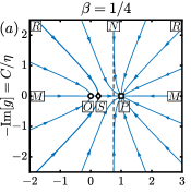
(a)

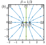
(b)

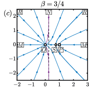
(c)

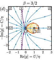
(d)

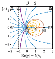
(e)

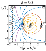
(f)

Figure 2: Phase portraits of equation (30), for six different values of $\beta>0$, $\beta\neq{1}$. Any given two trajectories that are symmetric with respect to the horizontal axis represent one possible similarity solution $f(\eta)=\eta\,{g(\eta)}$, with the origin of the trajectory denoting $\eta=0$ and the endpoint denoting $|\eta|\to\infty$. The three fixed points $O=(0,0)$ (stable node), $P=(1,0)$ (node), and $S=(\beta,0)$ (saddle) have horizontal and vertical eigendirections for all $\beta>0$. Points $M$, $N$, $R$ are the fixed points of the ODE satisfied by the reciprocals of the solution (see appendix A). Only green, purple, orange, and yellow trajectories represent similarity solutions that are physically relevant, as illustrated in table LABEL:tab:trajectories. Stability criteria (section LABEL:sec:stability) select the only five solutions that can be obtained in practice, which are highlighted with a wider streak. The dashed vertical line corresponds to $U/\eta=1-\beta$.

Phase portraits of the system are shown in figure 2, for a set of six representative values of $\beta$. The phase plane has a remarkably simple structure, being symmetric with respect to the horizontal axis $C/\eta=0$ due to the invariance of (30) to $g\to\bar{g}$. The plane always has two star nodes $O=(0,0)$ and $P=(1,0)$ at fixed positions along the horizontal axis, and one saddle point $S=(\beta,0)$ that lies between $O$ and $P$ for $0<\beta<1$ and to the right of $P$ for $\beta>1$. All three points $O$, $P$ and $S$ have horizontal and vertical eigendirections. These fixed points, as well as those of the ODE systems satisfied by the reciprocals $\eta/U$ and $\eta/C$ (which determine the behavior of trajectories as $U/\eta\to\pm\infty$ and/or $C/\eta\to\pm\infty$), are listed in table 3.1.

The beginning of each trajectory, either at infinity or at an unstable node, represents the origin $\eta=0$, while its end indicates the far field $|\eta|\to\infty$. The saddle $S$ represents a ‘front’ of the solution, where its derivative $f^{\prime}(\eta)$ exhibits a singularity and the concentration transitions between a region of $C(\eta)>0$ and a region where $C(\eta)=0$. As discussed above, any similarity solution $f(\eta)$ with a non-negative concentration $C(\eta)\geq{0}$ must be realized through the combination of two trajectories, one in the upper half plane $C(\eta)/\eta>0$ representing the solution for $\eta>0$, and its mirror image in the lower half plane $C(\eta)/\eta<0$, representing it for $\eta<0$. Such a combination also ensures that $f(\eta)$ that will have the required parity, i.e., $U(\eta)$ odd and $C(\eta)$ even. Furthermore, the leading-order asymptotic form of the solution around each of these points can be found via linearization (see Appendix A) and is also provided in table 3.1, listing all possible behaviors of $f(\eta)$ as $\eta\to 0$ and as $|\eta|\to\infty$ for different values of $\beta$. Since the similarity solution $f(\eta)$ is the result of ‘patching’ together two solutions $\eta\,g(|\eta|)$ and $\eta\,\bar{g}(|\eta|)$, the expansions around $\eta=0$ often involve terms like $\mathrm{sgn}\left(\eta\right)$ and $|\eta|$, which can only result in regular solutions for some specific values of $\beta$ as we show in section LABEL:sec:stability.

Fixed point	Type	Meaning	$U(\eta)\sim$	$C(\eta)\sim$
$\left(\dfrac{U}{\eta},\dfrac{C}{\eta}\right)$
$O$ $(0,0)$	SN	$|\eta|\to\infty$	$K\,\mathrm{sgn}\left(\eta\right)|\eta|^{\frac{\beta-1}{\beta}}$	0
			$K^{2}\cfrac{(\beta-1)}{\beta}\,\mathrm{sgn}\left(\eta\right)|\eta|^{\frac{\beta-2}{\beta}}$	$K|\eta|^{\frac{\beta-1}{\beta}}$
			$K\,\mathrm{sgn}\left(\eta\right)|\eta|^{\frac{\beta-1}{\beta}}$	$K^{\prime}|\eta|^{\frac{\beta-1}{\beta}}$
$P$ $(1,0)$	SN [$0<\beta<1$]	$|\eta|\to\infty$	$\eta+{K}\,\mathrm{sgn}\left(\eta\right)|\eta|^{\frac{\beta}{\beta-1}}$	0
	UN [$\beta>1$]	$\eta=0$	$\eta+\cfrac{K^{2}\beta}{(1-\beta)}\,\mathrm{sgn}\left(\eta\right)|\eta|^{\frac{\beta+1}{\beta-1}}$	$K|\eta|^{\frac{\beta}{\beta-1}}$
			$\eta+K\,\mathrm{sgn}\left(\eta\right)|\eta|^{\frac{\beta}{\beta-1}}$	$K^{\prime}|\eta|^{\frac{\beta}{\beta-1}}$
$S$ $(\beta,0)$	S	Front at $\eta=\eta_{f}$	$\beta\eta\pm\eta\ln^{\frac{1}{2}}\left(\left|\cfrac{\eta}{\eta_{f}}\right|^{2\beta(1-\beta)}\right)$	0
			$\beta\eta$	$|\eta|\ln^{\frac{1}{2}}\left(\left|\cfrac{\eta_{f}}{\eta}\right|^{2\beta(1-\beta)}\right)$
$M$ $(\pm\infty,0)$	S	$\eta=0$	$K\,\mathrm{sgn}\left(\eta\right)$	$0$
$N$ $(1-\beta,\pm\infty)$	S	$\eta=0$	$(1-\beta)\eta+\dfrac{\beta(1-\beta)(1-2\beta)}{3K^{2}}\eta^{3}$	$K-\dfrac{\beta(1-\beta)}{2K}\eta^{2}$
$R$ $(\pm\infty,\pm\infty)$	UN	$\eta=0$	$K\,\mathrm{sgn}\left(\eta\right)$	$K^{\prime}$

Table 1: Fixed points of the ODE system given by the real and imaginary parts of (30), for $\beta>0$ and $\beta\neq{1}$. SN denotes a stable node, UN an unstable node, and S a saddle. Points $M$, $N$ and $R$ are obtained as fixed points of ODE systems involving the reciprocals $\eta/U$ and $\eta/C$, as detailed in Appendix A. The entries for $U(\eta)$ and $C(\eta)$ denote every possible asymptotic expansion about each fixed point, where $K$ and $K^{\prime}$ are independent, real, nonzero constants of integration, and $\eta_{f}$ is the (real, nonzero) location of the front occurring at the saddle point $S$. When more than one entry for $U(\eta)$ and $C(\eta)$ is provided, the first two rows correspond to the eigendirections of the fixed point (i.e., the horizontal and vertical directions for $O$, $P$ and $S$), and the third (if provided) to generic curves.

While all possible similarity solutions with the correct parity can be placed in the plane, not all of them are necessarily relevant from a physical standpoint. The advantage of a phase plane formalism is that it provides a way to systematically classify all trajectories in terms of the fixed points that they connect, so that they can be identified as relevant or irrelevant.

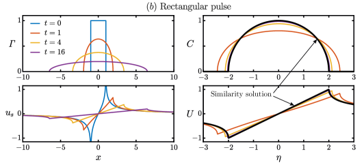
(b)

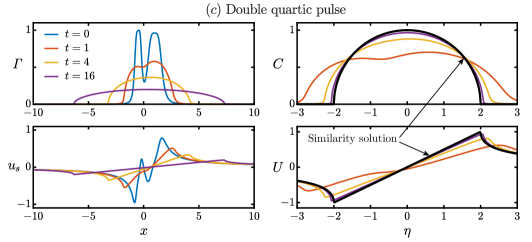
(c)

Figure 3: Spreading solutions with $Pe_{s}^{-1}=0$, for initial profiles of surfactant given by $(a)$ a Cauchy pulse, $(b)$ a rectangular pulse, and $(c)$ a double quartic pulse, with their functional forms given in Appendix E. For each example, left panels show the concentration $\Gamma(x,t)$ and interfacial velocity $u_{s}(x,t)$ obtained through the exact solution of (19), while right panels show the same data rescaled with the similarity variables given by (20) and (21). At nondimensional times $t\gg{1}$, all pulses converge towards the similarity solution (LABEL:eq:f_pulses_ReIm). For the double quartic pulse, the reference position in (20) is $x_{*}=1/2$; in all other examples $x_{*}=t_{*}=0$.

displays three distinct spreading pulses of surfactant (whose initial profiles $\Gamma_{0}(x)$ can be found in Appendix E) obtained solving the inviscid Burgers equation (19a) via the method of characteristics (Crowdy, 2021b). At large times $t\gg{1}$, the curves are shown to collapse onto the similarity solution (LABEL:eq:f_pulses), which is equivalent to the one originally identified by Thess (1996) through different methods. As pointed out by Bickel & Detcheverry (2022), a Cauchy pulse (figure LABEL:fig:spreading_no_diff_cauchy), which decays as $\Gamma\sim{x}^{-2}$ in the far field, requires very large times of order $t={O}(10^{3})$ to become visually indistinguishable from the similarity solution. However, figures 3b and 3c illustrate how pulses with a faster decay or compact support require much shorter times, $t={O}(10)$ to converge to (LABEL:eq:f_pulses).

It is worth noting that the initial profile $\Gamma_{0}(x)$ of the double quartic pulse of figure 3c is asymmetric, and therefore the center $x_{*}$ of the distribution at long times is nonzero. We show in Appendix C that the first moment of the surfactant distribution

$$M_{1}\vcentcolon=\int_{-\infty}^{\infty}x\Gamma(x,t)\,\mathrm{d}{x}=\int_{-\infty}^{\infty}x\Gamma_{0}(x)\,\mathrm{d}{x}$$ (65)

is a conserved invariant of the problem, provided the above integral exists. This leads to a straightforward definition of the reference position $x_{*}$ for pulses, namely

$$x_{*}=\dfrac{\int_{-\infty}^{\infty}x\Gamma_{0}(x)\,\mathrm{d}{x}}{\int_{-\infty}^{\infty}\Gamma_{0}(x)\,\mathrm{d}{x}}=\dfrac{M_{1}}{M_{0}}.$$ (66)

In the case of figure 3c, we have that $x_{*}=1/2$ (see Appendix E), as can be evidenced by the shifted pulse at long times in the top left panel.

4.2 General case with finite diffusion

For general values of $Pe_{s}^{-1}>0$, the similarity equation (23) requires values of $\alpha=-1/2$ and $\beta=1/2$. Incidentally, the additional requirement $\alpha+\beta=0$ from the integral constraint is also satisfied by these two values, illustrating that this more general case also displays self-similar solutions of the first kind. The governing ODE given by (24) can be integrated directly, leading to

$$\dfrac{\,\mathrm{d}f}{\,\mathrm{d}\eta}=k_{1}-\eta{f}+f^{2},$$ (67)

where the constant $k_{1}$ must be real since, at the origin, the solution $f(0)$ is imaginary and the derivative $f^{\prime}(0)$ is real. The far-field condition (29), which in this case with $\beta=1/2$ translates to $f\sim{k}_{+}\,\eta^{-1}$ as $\eta\to\infty$, can be introduced in (67) to obtain that $k_{1}=k_{+}$, meaning that the constant $k_{1}$ in (67) is simply the prefactor in the leading order far-field behavior of $f(\eta)$. This constant can be obtained realizing that, at the initial time $t\to{t}_{*}$, the solution must converge to a single Dirac distribution of surfactant with mass $M_{0}$ centered at $x_{*}$, and with an interfacial velocity that must be the Hilbert transform of that Dirac distribution. This can be stated mathematically as

$$A|t-t_{*}|^{-1/2}f(\eta)\sim\mathcal{H}\left[M_{0}\delta(x-x_{*})\right]-\mathrm{i}\,M_{0}\delta(x-x_{*})\quad\text{as }t\to{t}_{*}.$$ (68)

Using the linearity of the Hilbert transform, the fact that $\mathcal{H}\left[\delta(x)\right]=(\pi{x})^{-1}$ (King, 2009b) and the rescaling property $\delta(Kx)=\delta(x)/K$ of the Dirac distribution, we obtain

$$A|t-t_{*}|^{-1/2}f(\eta)\sim\dfrac{M_{0}}{A}|t-t_{*}|^{-1/2}\left[\dfrac{1}{\pi\eta}-\mathrm{i}\,\delta(\eta)\right]\quad\text{as }\eta\to\infty,$$ (69)

and, since we had chosen $A=\sqrt{2/Pe_{s}}$ in Section 2.1, this means that

$$f(\eta)\sim\dfrac{M_{0}Pe_{s}}{2\pi}\eta^{-1}\quad\text{as }\eta\to\infty.$$ (70)

Hence, the integration constant must be

$$k_{1}=k_{+}=\dfrac{M_{0}Pe_{s}}{2\pi}.$$ (71)

The ODE (67) can be further integrated by noting that it is a Riccati equation, which can be solved with the change of dependent variable

$$f=-\dfrac{1}{h}\dfrac{\,\mathrm{d}h}{\,\mathrm{d}\eta}=-\dfrac{\,\mathrm{d}}{\,\mathrm{d}\eta}\mathrm{Log}(h),$$ (72)

which leads to a linear equation

$$\dfrac{\,\mathrm{d}^{2}h}{\,\mathrm{d}\eta^{2}}+\eta\dfrac{\,\mathrm{d}h}{\,\mathrm{d}\eta}+k_{1}{h}=0.$$ (73)

Note the analogy between the Cole-Hopf transformation used to linearize Burgers equation directly (Bickel & Detcheverry, 2022) and the change of variable (72) to linearize the similarity ODE (67). The solution to equation (73) is

$$h(\eta)=k_{2}\,{}_{1}F_{1}\left(\dfrac{k_{1}}{2}\,;\dfrac{1}{2}\,;-\dfrac{\eta^{2}}{2}\right)+k_{3}\,\eta\,{}_{1}F_{1}\left(\dfrac{1}{2}+\dfrac{k_{1}}{2}\,;\dfrac{3}{2}\,;-\dfrac{\eta^{2}}{2}\right),$$ (74)

where ${}_{1}F_{1}\left(a\,;b\,;z\right)$ is Kummer’s confluent hypergeometric function (Olver et0al., 2010) and $k_{2}$, $k_{3}$ are complex integration constants. Since, as evidenced by the change of variables (72), the solution $f(\eta)$ is independent of any rescalings of $h(\eta)$ with a complex constant, we can set $k_{3}=1$ without any loss of generality. The remaining constant $k_{2}$ indicates the value of the concentration $C$ at the origin, since

$$f(0)=-\dfrac{1}{h(0)}\left.\dfrac{\,\mathrm{d}h}{\,\mathrm{d}\eta}\right|_{\eta=0}=-\dfrac{1}{k_{2}},$$ (75)

which highlights that $k_{2}$ must be imaginary with $\mathrm{Im}\left[k_{2}\right]<0$. The value of $k_{2}$ can be obtained imposing the integral constraint given by (LABEL:eq:integral_constraint_pulse), namely

$$\int_{-\infty}^{\infty}f\,\mathrm{d}{\eta}=-\int_{-\infty}^{\infty}\dfrac{\,\mathrm{d}}{\,\mathrm{d}\eta}\mathrm{Log}(h)\,\mathrm{d}{\eta}=-\mathrm{i}\,\dfrac{M_{0}Pe_{s}}{2},$$ (76)

which can be simplified as

$$\lim_{\eta\to\infty}\Bigl{[}\mathrm{Log}(h(\eta))-\mathrm{Log}(h(-\eta))\Bigr{]}=\mathrm{i}\,\dfrac{M_{0}Pe_{s}}{2}.$$ (77)

Since $k_{1}$ is real, $k_{2}$ is purely imaginary, $k_{3}=1$, and the hypergeometric functions in (74) are a function only of $\eta^{2}$, we can conclude that $h(-\eta)=-\bar{h}(\eta)$. Using this identity, and splitting $\mathrm{Log}(z)=\ln|z|+\mathrm{i}\mathrm{Arg}(z)$, we get

$$\lim_{\eta\to\infty}\mathrm{Arg}(h(\eta))=\dfrac{M_{0}Pe_{s}}{4}-\dfrac{\pi}{2}$$ (78)

which, after considering the far-field behavior of ${}_{1}F_{1}\left(a\,;b\,;z\right)$ (Olver et0al., 2010) and the fact that $k_{1}=M_{0}Pe_{s}/(2\pi)$, leads to

$$k_{2}=-\mathrm{i}\dfrac{\sqrt{2}}{2}\dfrac{\rmGamma\left(\dfrac{M_{0}Pe_{s}}{4\pi}\right)}{\rmGamma\left(\dfrac{1}{2}+\dfrac{M_{0}Pe_{s}}{4\pi}\right)},$$ (79)

where $\rmGamma\left(\,\,\right)$ is the gamma function and should not be confused with the surfactant concentration $\Gamma$, which is italicized throughout the paper. Undoing the change of variable (72), the final form of the similarity solution is

$$f(\eta)=\tfrac{6\,\rmGamma\left(\frac{1}{2}+\zeta\right){}_{1}F_{1}\left(\frac{1}{2}+\zeta\,;\frac{3}{2}\,;-\frac{\eta^{2}}{2}\right)+6\sqrt{2}\,\mathrm{i}\,\eta\,\rmGamma\left(1+\zeta\right){}_{1}F_{1}\left(1+\zeta\,;\frac{3}{2}\,;-\frac{\eta^{2}}{2}\right)-4\eta^{2}\,\rmGamma\left(\frac{3}{2}+\zeta\right){}_{1}F_{1}\left(\frac{3}{2}+\zeta\,;\frac{5}{2}\,;-\frac{\eta^{2}}{2}\right)}{3\sqrt{2}\,\mathrm{i}\,\rmGamma\left(\zeta\right){}_{1}F_{1}\left(\zeta\,;\frac{1}{2}\,;-\frac{\eta^{2}}{2}\right)-6\eta\,\rmGamma\left(\frac{1}{2}+\zeta\right){}_{1}F_{1}\left(\frac{1}{2}+\zeta\,;\frac{3}{2}\,;-\frac{\eta^{2}}{2}\right)},$$ (80a)

where we have defined

$$\zeta\vcentcolon=\dfrac{M_{0}Pe_{s}}{4\pi}.$$ (80b)

The solution given by (80) is equivalent to the fundamental solution derived by Bickel & Detcheverry (2022) using the Cole-Hopf transformation with a Dirac distribution as the initial condition. Figure 3.1

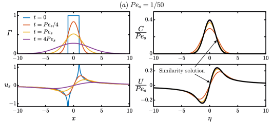
(a)

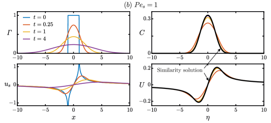
(b)

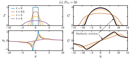
(c)

Figure 4: Spreading solutions for an initially rectangular pulse of surfactant, with a functional form given in Appendix E, for $(a)$ $Pe_{s}=1/50$, $(b)$ $Pe_{s}=1$, and $(c)$ $Pe_{s}=50$. For each example, left panels show the concentration $\Gamma(x,t)$ and interfacial velocity $u_{s}(x,t)$ obtained through the exact solution of (18), while right panels show the same data rescaled with the similarity variables given by (20) and (21). At nondimensional times $t\gg{1}$, all pulses converge towards the similarity solution given by (80). In all examples, $x_{*}=t_{*}=0$.

displays an initially rectangular pulse of surfactant spreading following Burgers equation (18a), for different values of the surface Péclet number. When advection is negligible and $Pe_{s}\ll{1}$, the solution quickly becomes Gaussian in shape, converging towards the fundamental solution of the (linear) diffusion equation. This occurs on times of order $t=O(Pe_{s})$, since at small $Pe_{s}$ the dominant balance in equation (18a) modifies the characteristic timescale, which we had assumed to be set by advection in Section 2. As $Pe_{s}$ increases and reaches an advection-dominated regime $Pe_{s}\gg{1}$, the solution changes shape, resembling the semicircular surfactant profile of the purely advective solution (LABEL:eq:f_pulses) of the previous subsection.

5 Filling solutions

In the case of filling solutions, sketched in figure 1b, there is no conserved mass of surfactant since the integral of $\Gamma_{0}(x)$ diverges as $\Gamma_{0}\to{1}$ in the far field. This leads to self-similar solutions of the second kind (Barenblatt, 1996), where the exponent $\beta$ cannot be determined from dimensional considerations, but is instead given by the stability criteria presented in section LABEL:sec:stability. Furthermore, the scaling constant $A$ is in this case dependent of the local properties of initial conditions, and can only be either computed numerically or calculated if a solution to (19) can be obtained explicitly. The four filling solutions identified in section 3 hold only locally, either before or after a reference time $t_{*}$ at which in the derivative of the solution is singular.

This singular behavior has only been observed (Thess et0al., 1997; Crowdy, 2021b; Bickel & Detcheverry, 2022) when the initial distribution of surfactant is zero $\Gamma_{0}(x)=0$ somewhere along the real line. Like in the well-studied case of real solutions of the inviscid Burgers equation (19a), the time $t_{*}$, position $x_{*}$, and velocity $u_{*}$ of the closure point (where the derivative of the solution in singular) can be calculated a priori from $\Gamma_{0}(x)$ using the method of characteristics, as detailed in appendix D. Similar arguments can be used to illustrate which initial conditions can be classified as ‘dimples’, leading to $\beta=2$, and which ones to ‘holes’, resulting in $\beta=3/2$. As shown in section LABEL:sec:stability, the key distinction between initial profiles $\Gamma_{0}(x)$ that lead to one or the other similarity solution is the second derivative of the solution at the singularity, which we can also calculate with the method of characteristics. To that end, we first define the (moving) position of the closure point as $x_{s}(t)\vcentcolon={x}_{*}-u_{*}(t_{*}-t)$. Then, we particularize the second derivative of the solution, given by equation (117), at $x_{s}(t)$ to obtain

$$\dfrac{\partial^{2}\psi}{\partial x^{2}}(x_{s}(t),t)=\dfrac{\psi_{0}^{\prime\prime}(x_{*}-t_{*}u_{*})}{\left(1+t\,\psi_{0}^{\prime}(x_{*}-t_{*}u_{*})\right)^{3}}.$$ (81)

In the case of real solutions, it can be shown that $\psi_{0}^{\prime\prime}(x_{*}-t_{*}\,u_{*})=0$ (see appendix D), and therefore $\partial_{xx}\psi=0$ for all times at the (moving) point of the shock. However, complex solutions can lead to either $\psi_{0}^{\prime\prime}(x_{*}-t_{*}u_{*})\neq{0}$, in which case we define the initial distribution $\Gamma_{0}(x)$ as a ‘dimple’, or to $\psi_{0}^{\prime\prime}(x_{*}-t_{*}u_{*})={0}$, in which case we define it as a ‘hole’. Each of these two cases lead to a different similarity solution and are therefore treated separately in the next two subsections.

5.1 Dimple solutions

The first dimple distribution we consider is $\Gamma_{0}(x)=x^{2}/(1+x^{2})$ (which we call the ‘Cauchy dimple’) since it has already been studied by Crowdy (2021b) and Bickel & Detcheverry (2022). It has a quadratic minimum $\Gamma_{0}(x)\sim{x}^{2}$ around $x=0$ and, since it is a symmetric distribution, it follows from the method of characteristics (see appendix D) that $u_{*}=x_{*}=0$ and $t_{*}=1$. The exact evolution of a Cauchy dimple is displayed in the left column of figure 5a,

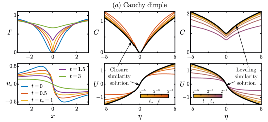
(a)

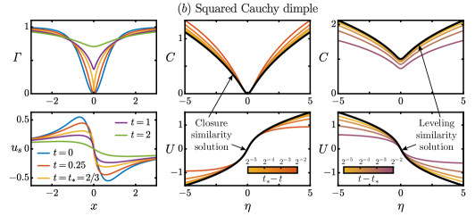
(b)

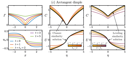
(c)

Figure 5: Filling solutions with $Pe_{s}^{-1}=0$, for initial ‘dimple’ distributions of surfactant given by $(a)$ a Cauchy dimple, $(b)$ a squared Cauchy dimple, and $(c)$ an arctangent dimple, with their functional forms given in appendix E. For each example, the left column shows the concentration $\Gamma(x,t)$ and interfacial velocity $u_{s}(x,t)$ obtained through the exact solution of (19). The middle and right columns show exact solutions rescaled in similarity variables (color curves), superimposed to the closure (89) and leveling (87) similarity solutions (black curves) valid prior and subsequent to the singularity, respectively. In all examples, $x_{*}=0$.

with the surfactant concentration reaching a cusp-like singularity at $t_{*}$ and $x_{*}$. The left column of figures 5b and 5c displays the evolution of other profiles $\Gamma_{0}(x)$ with different functional forms (detailed in appendix E), but always with a quadratic minimum to ensure that they display the same similarity behavior. Self-similarity appears locally, for positions and times close enough to $x_{*}$ and $t_{*}$, respectively. As discussed in section LABEL:sec:stability, the self-similar solution that appears prior to $t_{*}$ is dubbed the ‘closure’ solution, since here the concentration remains zero $\Gamma(x_{*},t)=0$ at all times. After the dimple ‘closes’ at $t_{*}$, a different ‘leveling’ solution appears, whereby the concentration starts leveling towards the final steady distribution $\Gamma(x,t)={1}$.

It is shown in section LABEL:sec:stability that the similarity exponent for dimple solutions is $\beta=2$, which can be substituted in the implicit similarity solution (32) to yield

$$\mathrm{Log}\left(1-\dfrac{f}{\eta}\right)-2\,\mathrm{Log}\left(\dfrac{f}{\eta}\right)-\ln|\eta|=k_{\pm}.$$ (82)

Like in section LABEL:sec:spreading_sols_no_diff, the logarithms can then be grouped accounting for a factor $2\pi\mathrm{i}$, and noting that $|\eta|=\mathrm{sgn}\left(\eta\right)\eta$ results in

$$\mathrm{Log}\left(\dfrac{\eta-f}{f^{2}}\right)=k_{\pm}\mathrm{sgn}\left(\eta\right)+2q\pi\mathrm{i},$$ (83)

with $q$ some integer. Exponentiation of both sides, and redefinition of the complex integration constant $e^{k_{\pm}+2q\pi\mathrm{i}}=e^{k_{\pm}}\to{k_{\pm}}$ leads to a quadratic equation

$$\mathrm{sgn}\left(\eta\right)k_{\pm}{f}^{2}+f-\eta=0.$$ (84)

Solutions to the quadratic equation (84) are valid both for (pre-singularity) closure solutions and for (post-singularity) leveling solutions. For both cases, we know that their expansions around $\eta=0$ are $f(\eta)\sim\eta-\mathrm{i}{K}\eta^{2}$ and $f(\eta)\sim-\mathrm{i}{K}-\eta$ from section 3, which both lead to imaginary constants $k_{\pm}$ when introduced in (84). Since $k_{-}=\bar{k}_{+}$, we have that $k_{-}=-k_{+}$ and we can consider a single constant $k=\mathrm{sgn}\left(\eta\right)k_{\pm}$. Solving (84),

$$f(\eta)=\dfrac{-1\pm\sqrt{1+4k\eta}}{2k}.$$ (85)

For the leveling solution, choosing the minus sign in (85) ensures that $C(0)>0$. This sign choice must be valid for all $\eta$ since a change from $-$ to $+$ requires the square root to be zero to maintain a continuous solution, while the radicand $1+4k\eta$ can never be zero with $k$ imaginary. We also fix $k=-\mathrm{i}$ so that $f(0)=-\mathrm{i}$ (or, equivalently, $C(0)=1$). The dimple leveling solution is then

$$f(\eta)=-\dfrac{\mathrm{i}}{2}\left[\sqrt{1-4\mathrm{i}\eta}+1\right],$$ (86)

which can alternatively be decomposed into its real and imaginary parts using the relation $\sqrt{z}=\sqrt{(|z|+\mathrm{Re}\left[z\right])/2}+\mathrm{i}\,\mathrm{sgn}\left(\mathrm{Im}\left[z\right]\right)\sqrt{(|z|-\mathrm{Re}\left[z\right])/2}$, leading to

$$C(\eta) =\dfrac{1}{2}\left\{\sqrt{\dfrac{1}{2}\left[\sqrt{1+16\eta^{2}}+1\right]}+1\right\},$$ (87a)

$$U(\eta) =-\dfrac{1}{2}\,\mathrm{sgn}\left(\eta\right)\sqrt{\dfrac{1}{2}\left[\sqrt{1+16\eta^{2}}-1\right]}.$$ (87b)

We note that (87) leads to $C(\eta)\sim(\sqrt{2}/2)\sqrt{|\eta|}$ and $U(\eta)\sim-\mathrm{sgn}\left(\eta\right)(\sqrt{2}/2)\sqrt{|\eta|}$ in the far field $|\eta|\to\infty$, compatible with (29).

For the closure solution, the choice in (85) must be the plus sign such that $f(0)=0$. In addition, we choose $k=\mathrm{i}$ such that the far-field behavior of the closure solution is equivalent to that of the leveling solution, leading to the same $C(\eta)\sim(\sqrt{2}/2)\sqrt{|\eta|}$ and to a velocity $U(\eta)\sim\mathrm{sgn}\left(\eta\right)(\sqrt{2}/2)\sqrt{|\eta|}$ with a flipped sign due to the reversal in the sign of $x$ between the definitions of the similarity variable (22a) and (22b) in each solution. The final form of the dimple closure solution is then

$$f(\eta)=-\dfrac{\mathrm{i}}{2}\left[\sqrt{1+4\mathrm{i}\eta}-1\right],$$ (88)

from which we obtain

$$C(\eta) =\dfrac{1}{2}\left\{\sqrt{\dfrac{1}{2}\left[\sqrt{1+16\eta^{2}}+1\right]}-1\right\},$$ (89a)

$$U(\eta) =\dfrac{1}{2}\,\mathrm{sgn}\left(\eta\right)\sqrt{\dfrac{1}{2}\left[\sqrt{1+16\eta^{2}}-1\right]}.$$ (89b)

The choice of (86) and (88) having an equivalent far-field behavior ensures that the multiplicative constant $A$ in the similarity formulation (20) is the same for both the closure and the leveling solutions. This fact simplifies calculations, since it then suffices to calculate $A$ for only one of the two solutions.

The middle column of figure 3.1 shows how the exact solutions converge to the closure self-similar profiles given by (88) before the singularity, for the three distinct initial profiles $\Gamma_{0}(x)$ considered. Likewise, the right-most column in figure 3.1 illustrates that exact solutions converge to the leveling solution (86) after the singularity. Since the similarity solutions are only valid locally, the agreement between the rescaled profiles is always improved as $t\to{t_{*}}$ or as $x\to{x_{*}}$.

5.2 Hole solutions

Contrary to dimples, hole similarity solutions (with $\beta=3/2$) had not yet been identified for the complex inviscid Burgers equation (19a). One of the simplest examples of a distribution of surfactant that satisfies this condition is a ‘rectangular hole’ with $\Gamma_{0}(x)=H(|x|-1)$, where $H(x)$ is the Heaviside step function, which we illustrate in figure 6a.

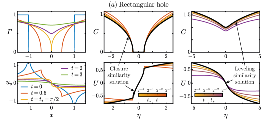
(a)

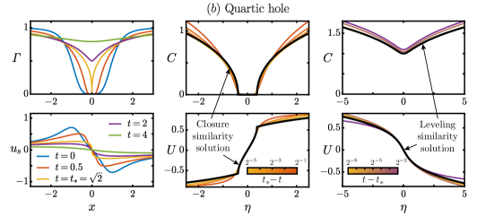
(b)

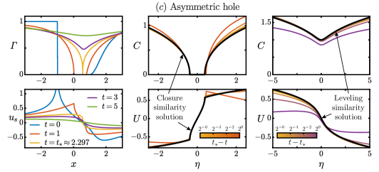
(c)

Figure 6: Filling solutions with $Pe_{s}^{-1}=0$, for initial ‘hole’ distributions of surfactant given by $(a)$ a rectangular hole, $(b)$ a quartic hole, and $(c)$ an asymmetric hole, with their functional forms given in appendix E. For each example, the left column shows the concentration $\Gamma(x,t)$ and interfacial velocity $u_{s}(x,t)$ obtained through the exact solution of (19). The middle and right columns show exact solutions rescaled in similarity variables (color curves), superimposed to the closure (98) and leveling (94) similarity solutions (black curves) valid prior and subsequent to the singularity, respectively. The asymmetric hole has $x_{*}\approx{0.562}$, otherwise $x_{*}=0$.

For this case, the initial surfactant profile is even and therefore its Hilbert transform $u_{s0}(x)=\mathcal{H}\left[\Gamma_{0}(x)\right]$ is odd, which implies (see appendix D) that the position of the singularity is $x_{*}=0$, its velocity $u_{*}=0$, and the closure time $t_{*}=\pi/2$. From this, one can easily verify that $\Gamma_{0}^{\prime\prime}(0)=u_{s0}^{\prime\prime}(0)=0$ and thus the condition for hole self-similar solutions $\psi_{0}^{\prime\prime}(x_{*}-u_{*}t_{*})=\psi_{0}^{\prime\prime}(0)=0$ is satisfied. Figure 6a depicts the exact evolution of the rectangular hole according to the inviscid Burgers equation (19a). Like for the case of dimples, the distribution first goes through a ‘closure’ phase where surfactant is advected inwards but the surfactant at the origin remains $\Gamma(0,t)=0$. However, it is easy to see in figure 6a that the self-similar dynamics before the closure time $t_{*}$ must be different from those of the dimple, since the solution always retains a finite interval around $x_{*}=0$ where the concentration remains zero. After the closure time $t_{*}=\pi/2$, the concentration at the origin starts ‘leveling’, with $\Gamma(0,t)>0$, until the profile reaches a homogeneous distribution $\Gamma(x,t)=1$ as $t\to\infty$.

In this case, the self-similar solutions can also be obtained in closed form by substituting $\beta=3/2$ in the implicit solution given by (32), which leads to

$$\mathrm{Log}\left(1-\dfrac{f}{\eta}\right)-3\,\mathrm{Log}\left(\dfrac{f}{\eta}\right)-\ln\left(\eta^{2}\right)=2k_{\pm}.$$ (90)

The integer prefactor allows to group the logarithms and obtain

$$\mathrm{Log}\left(\dfrac{\eta-f}{f^{3}}\right)=2k_{\pm}+2q\pi,$$ (91)

with $q$ an integer. Exponentiation, noting that $e^{2k+2q\pi}=e^{2k}$, and redefinition of the integration constants leads to a cubic equation, valid both for closure and leveling,

$$k_{\pm}f^{3}+f-\eta=0.$$ (92)

In the case of the leveling solution, $k_{\pm}$ must be real for $f(0)$ to be imaginary. For the closure solution, introducing the expansion $f(\eta)\sim\eta+K\eta^{3}$ in (92) also leads to real constants and thus, since $k_{-}=\bar{k}_{+}$, for either solution we can consider a single constant $k=k_{-}=k_{+}$, as in the case of spreading pulse solutions of section LABEL:sec:spreading_sols_no_diff.

We first solve (92) for the case of the (post-singularity) leveling solution. We again choose to fix $f(0)=-\mathrm{i}$, or equivalently $C(0)=1$, which results in $k=1$. The discriminant of the cubic (92) is then $-4-27\eta^{2}$, which is negative for any $\eta$. This implies that (92), for any given value of $\eta$, has one real and two complex conjugate solutions that can be obtained using standard methods for solving cubic equations (Cox, 2012). Choosing the complex solution with a negative imaginary part (such that $C(\eta)>0$) results in the hole leveling solution

$$f(\eta)=e^{-\frac{\pi\mathrm{i}}{3}}\sqrt[3]{\dfrac{1}{2}\left[\sqrt{\eta^{2}+\dfrac{4}{27}}-\eta\right]}+e^{-\frac{2\pi\mathrm{i}}{3}}\sqrt[3]{\dfrac{1}{2}\left[\sqrt{\eta^{2}+\dfrac{4}{27}}+\eta\right]}.$$ (93)

Furthermore, since the arguments of the two cubic roots in (93) are always real and positive, it is straightforward to decompose the expression into

$$C(\eta) = \,\,\dfrac{\sqrt{3}}{2} \left\{\sqrt[3]{\dfrac{1}{2}\left[\sqrt{\eta^{2}+\dfrac{4}{27}}-\eta\right]}+\sqrt[3]{\dfrac{1}{2}\left[\sqrt{\eta^{2}+\dfrac{4}{27}}+\eta\right]}\right\},$$ (94a)

$$U(\eta) = \dfrac{1}{2} \left\{\sqrt[3]{\dfrac{1}{2}\left[\sqrt{\eta^{2}+\dfrac{4}{27}}-\eta\right]}-\sqrt[3]{\dfrac{1}{2}\left[\sqrt{\eta^{2}+\dfrac{4}{27}}+\eta\right]}\right\},$$ (94b)

where the far-field behavior $|\eta|\to\infty$ is in this case given by $C(\eta)\sim(\sqrt{3}/2)\sqrt[3]{|\eta|}$ and $U(\eta)\sim-\,\mathrm{sgn}\left(\eta\right)(1/2)\sqrt[3]{|\eta|}$.

In the case of the closure solution, we choose the integration constant such that the far-field behavior of the closure solution is equivalent to that of the leveling solution which, as we show below, requires $k=-1$. As in the case of dimples, this choice of far field ensures that the scaling constant $A$ in the similarity formulation (20) is the same for both closure and leveling. The discriminant of (92) is then $4-27\eta^{2}$, which indicates that its three solutions are real for $|\eta|\leq\sqrt{4/27}=2\sqrt{3}/9$, whereas for $|\eta|\geq 2\sqrt{3}/9$ there is one real and two complex conjugate solutions. The only way to ensure a continuous solution with $C(\eta)>0$ is to define $f(\eta)$ piecewise, with one of the three solutions of the cubic valid for $\eta\leq 2\sqrt{3}/9$, and another one valid for $\eta\geq 2\sqrt{3}/9$. Such a solution is

$$f(\eta)=\begin{cases}e^{\frac{\pi\mathrm{i}}{3}}\left(\sqrt[3]{\phantom{-}\dfrac{1}{2}\left[\sqrt{\eta^{2}-\dfrac{4}{27}}+\eta\right]}-\sqrt[3]{\phantom{-}\dfrac{1}{2}\left[\sqrt{\eta^{2}-\dfrac{4}{27}}-\eta\right]}\,\,\right)&\text{if }\eta\leq\dfrac{2\sqrt{3}}{9},\\[20.0pt] e^{\frac{\pi\mathrm{i}}{3}}\left(\sqrt[3]{-\dfrac{1}{2}\left[\sqrt{\eta^{2}-\dfrac{4}{27}}-\eta\right]}-\sqrt[3]{-\dfrac{1}{2}\left[\sqrt{\eta^{2}-\dfrac{4}{27}}+\eta\right]}\,\,\right)&\text{if }\eta\geq\dfrac{2\sqrt{3}}{9},\end{cases}$$ (95)

which can be expressed more compactly realizing that, for any real number $\lambda>0$,

$$\sqrt{\left(\lambda-\eta\right)}\sqrt{-\left(\lambda+\eta\right)}=\begin{cases}\sqrt{\eta^{2}-\lambda}&\text{if }\eta\leq\lambda,\\[10.0pt] -\sqrt{\eta^{2}-\lambda}&\text{if }\eta\geq\lambda.\end{cases}$$ (96)

We then use this expression to obtain a hole closure solution that is not defined piecewise,

$$f(\eta)=e^{\frac{\pi\mathrm{i}}{3}}\left\{\quad\sqrt[3]{\frac{1}{2}\left[\sqrt{\left(\frac{2\sqrt{3}}{9}-\eta\right)}\sqrt{-\left(\frac{2\sqrt{3}}{9}+\eta\right)}+\eta\right]}\right.-\\ \left.-\sqrt[3]{\dfrac{1}{2}\left[\sqrt{\left(\dfrac{2\sqrt{3}}{9}-\eta\right)}\sqrt{-\left(\dfrac{2\sqrt{3}}{9}+\eta\right)}-\eta\right]}\quad\right\}.$$ (97)

For $|\eta|\geq 2\sqrt{3}/9$, the argument of the cubic roots in (97) is always real, leading to a straightforward decomposition into real and imaginary parts. However, in the case of $|\eta|\leq 2\sqrt{3}/9$, the real and imaginary parts of the solution can only be obtained through the trigonometric solution of the cubic (Cox, 2012). In summary, the final form of the similarity solutions $C(\eta)$ and $U(\eta)$ is

$$C(\eta) =\begin{cases}0&\text{for }|\eta|\leq\dfrac{2\sqrt{3}}{9},\\[15.0pt] \dfrac{\sqrt{3}}{2}\left(\sqrt[3]{\dfrac{1}{2}\left[|\eta|+\sqrt{\eta^{2}-\dfrac{4}{27}}\right]}-\sqrt[3]{\dfrac{1}{2}\left[|\eta|-\sqrt{\eta^{2}-\dfrac{4}{27}}\right]}\,\right)&\text{for }|\eta|\geq\dfrac{2\sqrt{3}}{9},\end{cases}$$ (98a)

$$U(\eta) =\begin{cases}\dfrac{2\sqrt{3}}{3}\,\sin\left[\dfrac{1}{3}\arcsin\left(\dfrac{3\sqrt{3}}{2}\,\eta\right)\right]&\text{for }|\eta|\leq\dfrac{2\sqrt{3}}{9},\\[15.0pt] \dfrac{1}{2}\,\mathrm{sgn}\left(\eta\right)\left(\sqrt[3]{\dfrac{1}{2}\left[|\eta|+\sqrt{\eta^{2}-\dfrac{4}{27}}\right]}+\sqrt[3]{\dfrac{1}{2}\left[|\eta|-\sqrt{\eta^{2}-\dfrac{4}{27}}\right]}\,\right)&\text{for }|\eta|\geq\dfrac{2\sqrt{3}}{9},\end{cases}$$ (98b)

where we can now confirm that its far field, which is given by $C(\eta)\sim(\sqrt{3}/2)\sqrt[3]{|\eta|}$ and $U(\eta)\sim\mathrm{sgn}\left(\eta\right)(1/2)\sqrt[3]{|\eta|}$, is equivalent to that of the leveling solution.

The center and right columns of figure 6a show that the exact solution, when appropriately rescaled using (20), converges to the closure solution (98) before $t_{*}$ and to the leveling solution (94) after $t_{*}$. Other initial surfactant profiles also lead to these similarity solutions, as long as the condition $\psi_{0}^{\prime\prime}(x_{*}-t_{*}u_{*})=0$ is met. It is worth noting that the initial surfactant distribution does not need to be zero at a finite interval to tend to a self-similar solution for a hole, as exemplified by the ‘quartic hole’ initial condition $\Gamma_{0}(x)=x^{4}/(1+x^{4})$, whose evolution is displayed in figure 6b. This initial profile also has even symmetry, leading to $x_{*}=0$, $u_{*}=0$, and $t_{*}=\sqrt{2}$ (see appendix D), but its initial concentration is zero only at the origin $x_{*}=0$. Regardless, since $\psi_{0}^{\prime\prime}(x_{*}-u_{*}t_{*})=\psi_{0}^{\prime\prime}(0)=0$, the self-similar dynamics also lead to the solutions given by the hole solutions (97) for $t<t_{*}$ (center column in figure 6b) and (93) for $t>t_{*}$ (right column). Even though the initial profile is zero at a single point, the self-similar dynamics dictate that the concentration profile ‘flattens’ as $t\to{t_{*}}$ to converge towards a solution that is zero at a finite interval.

The last example illustrated in figure 6c is an asymmetric initial condition. For this case, we have that $x_{*}\neq{0}$ and $u_{*}\neq{0}$, although their values can still be calculated from the method of characteristics, as detailed in appendix D. The self-similar dynamics are still governed by the solutions (97) and (93) although, since the point of the singularity moves with $u_{*}\neq{0}$, the self-similar variable must be corrected for a frame of reference moving with the closure point. This leads to a more general similarity ansatz

$$\psi(x,t) =u_{*}+A|t-t_{*}|^{\beta-1}f(\eta),$$ (99a)

$$\eta =\mathrm{sgn}\left(t-t_{*}\right)\dfrac{x-\left[x_{*}+u_{*}(t-t_{*})\right]}{A|t-t_{*}|^{\beta}}.$$ (99b)

Equation (99) accounts for the moving closure point, whose position is $x_{s}(t)=x_{*}+u_{*}(t-t_{*})$. Note that $x_{s}(t_{*})=x_{*}$, whereas $x_{s}(0)=x_{*}-u_{*}t_{*}$, which is the departure point of the moving closure point.

6 Conclusions

Quantitatively describing Marangoni flows induced by surfactant is a central problem in interfacial fluid dynamics, due to their prevalence in environmentally and industrially relevant multiphase flows. Motivated by recent theoretical progress, we have investigated the two-dimensional spreading problem for a deep, viscous fluid subphase in terms of its self-similarity. The analysis reveals a beautiful structure with six distinct similarity solutions and three different exponents $\beta$, which we list in table 3,

Name	$Pe_{s}^{-1}$	Kind	Validity	Exponent $\beta$	Similarity variable $\eta$	Solution $f(\eta)$
Pulse	0	First	$t\gg{1}$	1/2	$\dfrac{x-x_{*}}{\left(\dfrac{M_{0}}{\pi}\,t\right)^{1/2}}$	(LABEL:eq:f_pulses)
Pulse	$>0$	First	$t\gg{1}$	1/2	$\dfrac{x-x_{*}}{\left(\dfrac{2}{Pe_{s}}\,t\right)^{1/2}}$	(80)
Dimple closure	0	Second	$t\lesssim{t_{*}}$	2	$\dfrac{[x_{*}+u_{*}(t-t_{*})]-x}{A(t_{*}-t)^{2}}$	(88)
Dimple leveling	0	Second	$t\gtrsim{t_{*}}$	2	$\dfrac{x-[x_{*}+u_{*}(t-t_{*})]}{A(t-t_{*})^{2}}$	(86)
Hole closure	0	Second	$t\lesssim{t_{*}}$	3/2	$\dfrac{[x_{*}+u_{*}(t-t_{*})]-x}{A(t_{*}-t)^{3/2}}$	(97)
Hole leveling	0	Second	$t\gtrsim{t_{*}}$	3/2	$\dfrac{x-[x_{*}+u_{*}(t-t_{*})]}{A(t-t_{*})^{3/2}}$	(93)

Table 3: Summary of the six similarity solutions found in this study, indicating the equation number of each solution $f(\eta)$ obtained in closed form. Here, $M_{0}$ is the dimensionless surfactant mass as defined in (110), and $Pe_{s}$ is the Péclet number given by (17). In the case of pulses, the reference position $x_{*}$ is the center of mass of the surfactant distribution given by (66), and in the case of dimples and holes $x_{*}$ is the ‘closure position’ at which the solution has a weak singularity, which can be calculated a priori from the initial conditions as described in appendix D. The parameters $t_{*}$ and $u_{*}$ are the closure time and instantaneous velocity of the closure point, respectively, and can also be calculated a priori using appendix D. For solutions of the second kind, the constant $A$ depends on local properties of the initial condition $\Gamma_{0}(x)$.

all of which can be obtained in closed from.

In section LABEL:sec:spreading_sols, we derive one similarity solution without diffusion ($Pe_{s}^{-1}=0$) and another with diffusion ($Pe_{s}^{-1}>0$) for the case of pulses of surfactant, both of which are valid at long times $t\gg{1}$. These two solutions are equivalent to the ones previously identified by Thess (1996) and Bickel & Detcheverry (2022), respectively, through different methods. In addition to their derivation, we have also shown (appendix C) how to calculate the center of mass $x_{*}$ around which these solutions appear, something particularly useful when the initial surfactant distribution is asymmetric or the combination of several pulses. Since their similarity exponent is $\beta=1/2$, these pulse solutions are analogous to a diffusive process where the surfactant peak decreases as $\Gamma\propto{t}^{-1/2}$, and its front spreads as $x_{f}\propto{t}^{1/2}$. These two solutions can therefore be used to obtain effective surfactant diffusivities resulting from the Marangoni flow, as detailed by Bickel & Detcheverry (2022). We also note that the solutions $N\to{O}$ in the phase plane (figure 2) that have $1/2<\beta<1$ are also spreading and, in principle, physically admissible in terms of their stability (section LABEL:sec:stability). Therefore, we postulate that surfactant pulses that decay too slowly in the far field to have a well-defined mass $M_{0}$ might display this kind of self-similar solution.

Section 5 is concerned with surfactant distributions that are locally depleted and flow inwards, for which similarity only occurs for $Pe_{s}^{-1}=0$. We have provided the first derivation of two similarity solutions with $\beta=2$, whose behavior had only been inferred from numerical simulations by Thess et0al. (1997). We have also derived two new similarity solutions with $\beta=3/2$, an exponent that had not been identified previously. Through insights provided by stability analysis (section LABEL:sec:stability) and the complex method of characteristics, we have also provided a quantitative criterion to determine if a given initial surfactant profile will develop similarity with $\beta=2$, in which case we call such profile a ‘dimple’, or with $\beta=3/2$, in which case we call it a ‘hole’. Aside from providing valuable information about the spatial and temporal structure of the evolution of surfactant, these solutions also allow to calculate effective local properties of the flow. For example, from the similarity ansatz (20a), we can deduce that the concentration at the centerline $x_{*}$ of an interfacial strip that is depleted of surfactant is

$$\Gamma(x_{*},t)=\begin{cases}0&\text{if }0\leq{t}\leq{t}_{*},\\ A(t-t_{*})&\text{if }{t}\gtrsim{t}_{*},\end{cases}$$ (100a)

for dimples, while for holes

$$\Gamma(x_{*},t)=\begin{cases}0&\text{if }0\leq{t}\leq{t}_{*},\\ A(t-t_{*})^{1/2}&\text{if }{t}\gtrsim{t}_{*},\end{cases}$$ (101a)

where we note that $t_{*}$ can be obtained exactly if the initial surfactant profile is known, as detailed in appendix D.

Since local surfactant concentrations are challenging to measure experimentally, one can also derive expressions for the centerline interfacial shear, which reads

$$\dfrac{\partial u_{s}}{\partial x}(x_{*},t)=\begin{cases}\dfrac{1}{t_{*}-t}&\text{if }{t}\lesssim{t}_{*},\\[10.0pt] \dfrac{1}{t-t_{*}}&\text{if }{t}\gtrsim{t}_{*},\end{cases}$$ (102a)

for dimples, and

$$\dfrac{\partial u_{s}}{\partial x}(x_{*},t)=\begin{cases}\dfrac{1}{t_{*}-t}&\text{if }{t}\lesssim{t}_{*},\\[10.0pt] \dfrac{1}{2(t-t_{*})}&\text{if }{t}\gtrsim{t}_{*},\end{cases}$$ (103a)

for holes. These expressions for the interfacial shear are in principle obtainable by measuring the interfacial velocity field in experiments, and should be valid for times sufficiently near $t_{*}$, but not too close to the singularity for surface diffusion to locally regularize the interfacial velocity field. The expressions do not depend on any scaling constant $A$, and the only parameter involved, $t_{*}$, can be either calculated exactly if the detailed spatial profile of the initial concentration is known, or measured from experimental data.

The taxonomy of self-similar solutions derived here provides insights into the behavior of Marangoni flows in the physical regime of interest, independently of the specific initial conditions. Some natural questions arise from this analysis, like the robustness of these solutions to physical effects like a finite surface diffusion or small amounts of endogenous surfactant (as in Grotberg et0al., 1995). While a finite surface diffusion, no matter how small, would always regularize the singularities in the solution derivatives, preliminary simulations confirm that the similarity solutions without diffusion ($Pe_{s}^{-1}=0$) provide a reasonable approximation of the dynamics, which is improved as $Pe_{s}\to\infty$. A detailed account on the rate of convergence of solutions with diffusion to the similarity solutions with $Pe_{s}^{-1}=0$, which could perhaps be achieved perturbatively, is left for future work. Similarly, it is worth asking if a self-similarity approach would yield similar insights in an axisymmetric geometry, since this work deals exclusively with a planar, two-dimensional domain. Axisymmetric distributions have a more complicated nonlocal closure relationship (Bickel & Detcheverry, 2022) for which it appears that no local reformulations like Burgers equation exist, but the tools of self-similarity can be nevertheless applied for nonlocal problems (as in Lister & Kerr, 1989, for example).

Acknowledgements

F. T-C. acknowledges support from a Distinguished Postdoctoral Fellowship from the Andlinger Center for Energy and the Environment.

Declaration of interests

The authors report no conflict of interest.

Appendix A Construction of the phase plane

We first recast the autonomous ODE (30), which governs the behavior of the complex similarity solution $f(\eta)=\eta\,{g}(\eta)$ in the limit $Pe_{s}^{-1}=0$, as

$$\dfrac{\,\mathrm{d}g}{\,\mathrm{d}\ln|\eta|}=\dfrac{g(1-g)(\bar{g}-\beta)}{|g-\beta|^{2}},$$ (104)

with the overbar indicating complex conjugation. Since the right-hand side of the above ODE has a singularity at $g=\beta$, we reparametrize the equation (as in, for instance, Slim & Huppert, 2004) in terms of an auxiliary variable $\chi$, leading to

$$\dfrac{\,\mathrm{d}g}{\,\mathrm{d}\chi} =g(1-g)(\bar{g}-\beta),$$ (105a)

$$\dfrac{\,\mathrm{d}\ln|\eta|}{\,\mathrm{d}\chi} =|g-\beta|^{2}.$$ (105b)

Since, by virtue of equation (105b) above, we have that

$$\dfrac{\,\mathrm{d}\ln|\eta|}{\,\mathrm{d}\chi}\geq 0,$$ (106)

then integrating the system in terms of $\chi$ instead of $\ln|\eta|$ does not change the direction of trajectories in the phase space $(\mathrm{Re}\left[g\right],-\mathrm{Im}\left[g\right])$, unlike in other more complicated systems of equations such as the one considered in Slim & Huppert (2004). The three fixed points of equation (105a) are given by $g=0$, $g=1$ and $g=\beta$, and linearization around each of them (Strogatz, 2018) reveals their type, as well as the asymptotic form of the solution around each of them (points $O$, $P$ and $S$ in table 3.1).

We integrate (105) in $\chi$ numerically using the built-in MATLAB integrator ode15s. The initial condition of (105b) is chosen as $\left.(\ln|\eta|)\right|_{\chi=0}=-K$, with $K\gg{1}$ to represent a point close to the origin $\eta\approx{0}$. The initial values of $g$ are seeded close to the fixed points of the system such that $g(\chi=0)=g_{0}+{\Delta}e^{i\theta}$, with $\Delta\ll{1}$ and $\theta$ real constants, and where $g_{0}$ is the value of $g$ at each fixed point. We integrate (105a) forward in $\chi$ if $g(\chi=0)$ lies on an unstable direction around the fixed point, and backward in $\chi$ if $g(\chi=0)$ lies on a stable direction. Integration proceeds until $\ln|\eta|$ reaches a target value $\ln|\eta|=K\gg{1}$, which represents the far field $|\eta|\to\infty$. The resulting trajectories are shown in figure 2.

We also consider the behavior of trajectories in the phase plane as $|g|\to\infty$, which can be illustrated by studying the fixed points of the dynamical system given by the reciprocals $1/\mathrm{Re}\left[g\right]=\eta/U$ and $-1/\mathrm{Im}\left[g\right]=\eta/C$. Splitting the complex ODE (30) into its real and imaginary parts, and changing variables $\tilde{u}\vcentcolon={1}/\mathrm{Re}\left[g\right]$ and $\tilde{c}\vcentcolon=-1/\mathrm{Im}\left[g\right]$, we obtain the system of ODEs:

$$\dfrac{\,\mathrm{d}\tilde{u}}{\,\mathrm{d}\ln|\eta|} =\tilde{u}\,\dfrac{\left[\tilde{u}^{2}(1+(\beta-1)\tilde{u})-\tilde{c}^{2}(\tilde{u}-1)(1-\beta\tilde{u})\right]}{\tilde{u}^{2}+\tilde{c}^{2}(1-\beta\tilde{u})^{2}},$$ (107a)

$$\dfrac{\,\mathrm{d}\tilde{c}}{\,\mathrm{d}\ln|\eta|} =\tilde{c}\,\dfrac{\left[\tilde{u}^{2}+\tilde{c}^{2}(1-2\beta\tilde{u}+\beta\tilde{u}^{2})\right]}{\tilde{u}^{2}+\tilde{c}^{2}(1-\beta\tilde{u})^{2}}.$$ (107b)

The fixed points of the system given by (107) are $(\tilde{u},\tilde{c})=(0,0)$, which represents $(\mathrm{Re}\left[g\right],-\mathrm{Im}\left[g\right])\to(\pm\infty,\pm\infty)$, and $(\tilde{u},\tilde{c})=((1-\beta)^{-1},0)$, which represents $(\mathrm{Re}\left[g\right],-\mathrm{Im}\left[g\right])\to(1-\beta,\pm\infty)$. Linearization around these two points leads to the rows of table 3.1 corresponding to points $N$ and $R$.

Finally, the behavior of solutions for $\mathrm{Re}\left[g\right]\to\pm\infty$ and $-\mathrm{Im}\left[g\right]=0$ can only be determined by examining the dynamical system given by the reciprocal $1/\mathrm{Re}\left[g\right]=\eta/U$ and the imaginary part $-\mathrm{Im}\left[g\right]$. Changing variables $\tilde{u}\vcentcolon={1}/\mathrm{Re}\left[g\right]$ and $\hat{c}\vcentcolon=-\mathrm{Im}\left[g\right]$, we obtain a dynamical system given by

$$\dfrac{\,\mathrm{d}\tilde{u}}{\,\mathrm{d}\ln|\eta|} =\tilde{u}\,\dfrac{\left[\tilde{u}\hat{c}^{2}(1+(\beta-1)\tilde{u})-(\tilde{u}-1)(1-\beta\tilde{u})\right]}{(1-\beta\tilde{u})^{2}+\tilde{u}^{2}\hat{c}^{2}},$$ (108a)

$$\dfrac{\,\mathrm{d}\hat{c}}{\,\mathrm{d}\ln|\eta|} =\hat{c}\,\dfrac{\left[1-2\beta\tilde{u}+\beta\tilde{u}^{2}+\tilde{u}^{2}\hat{c}^{2}\right]}{(1-\beta\tilde{u})^{2}+\tilde{u}^{2}\hat{c}^{2}}.$$ (108b)

The only fixed point of (108) is $(\tilde{u},\hat{c})=(0,0)$, which represents $(\mathrm{Re}\left[g\right],-\mathrm{Im}\left[g\right])\to(\pm\infty,0)$. Linearization of (108) around this point results in the row of table 3.1 corresponding to point $M$.

Appendix B Interpretation of the phase plane

In order to interpret the phase plane in figure 2, it is useful to note two facts about the sign of solutions. First, from the self-similar ansatz (21b) and the fact that $\alpha=\beta-1$, we have at the origin $x=x_{*}$ that $\Gamma(x_{*},t)=A|t-t_{*}|^{\beta-1}C(0)$, illustrating that, if $C(0)>{0}$, values of $0<\beta<1$ will result in surfactant locally decreasing in time (i.e., spreading solutions), whereas exponents $\beta>1$ represent locally increasing surfactant (i.e. filling solutions). Consequently, solutions with $0<\beta<1$ must lead to a (locally) outward flow as in figure 1a, with $u_{s}$ positive for $x>x_{*}$ and $u_{s}$ negative for $x<x_{*}$ or, in other words, $(x-x_{*})u_{s}>0$. On the other hand, solutions with $\beta>1$ must lead to $(x-x_{*})u_{s}<0$ locally around the origin as in figure 1b.

Second, physical solutions require $\Gamma(x,t)\geq{0}$ and therefore also $C(\eta)\geq{0}$. Since each quadrant of the phase plane has a fixed sign of $C(\eta)/\eta$ and $U(\eta)/\eta$, it then follows that each quadrant must also have a fixed sign of $\eta$ and $U(\eta)$ individually. These sign restrictions lead to a unique meaning for each quadrant of the phase plane, as illustrated in figure 7.

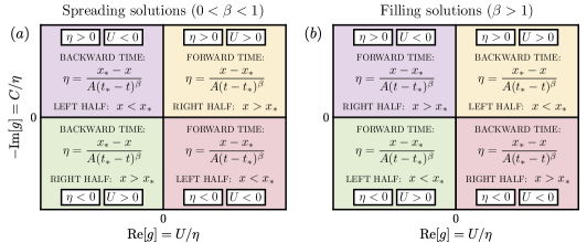
Figure 7: Physical interpretation of each quadrant of the phase plane in figure 2, for $(a)$ spreading solutions with an outward flow (as in figure 1a), and $(b)$ filling solutions with an inward flow (as in figure 1b). In order for the concentration $\Gamma(x,t)$ to be strictly non-negative, each quadrant must correspond to a specific definition of the similarity variable, either forward-time as in equation (22a) or backward-time as in equation (22b). In addition, each quadrant represents one half of the real line, either $x>x_{*}$ or $x<x_{*}$.

For a given value of $\beta$, each quadrant must represent either a forward-time (22a) or backward-time (22b) scaling, as well as necessarily belong to either the right half of the real line (i.e., $x>x_{*}$), or to the left half (i.e., $x<x_{*}$).

Appendix C Invariants of the problem

Direct integration of the surfactant conservation law given by equation (3) yields

$$\dfrac{\,\mathrm{d}}{\,\mathrm{d}t}\int_{-\infty}^{\infty}\Gamma\,\mathrm{d}{x}+\left.\left(u_{s}\Gamma\right)\right|_{-\infty}^{\infty}=\dfrac{1}{Pe_{s}}\left.\dfrac{\partial\Gamma}{\partial x}\right|_{-\infty}^{\infty}$$ (109)

and, since $u_{s}(x,t)$ necessarily decays and $\Gamma(x,t)$ can be at most constant in the far field, we then have that

$$\dfrac{\,\mathrm{d}}{\,\mathrm{d}t}\int_{-\infty}^{\infty}\Gamma\,\mathrm{d}{x}=0.$$ (110)

Equation (110) implies that the total mass $M_{0}$ of surfactant, as defined in (LABEL:eq:def_M0), is conserved in time. This holds as long as the integral given by (LABEL:eq:def_M0) exists, which is the case for initial pulses of surfactant with $\Gamma_{0}(x)$ decaying sufficiently quickly as $|x|\to\infty$.

The surfactant mass $M_{0}$ is, however, not the only invariant for this particular problem. Multiplying (3) by $x$ and applying the chain rule, we obtain

$$\dfrac{\partial\left(x\Gamma\right)}{\partial t}+\dfrac{\partial}{\partial x}\left(xu_{s}\Gamma\right)-u_{s}\Gamma=\dfrac{1}{Pe_{s}}\left[\dfrac{\partial}{\partial x}\left(x\dfrac{\partial\Gamma}{\partial x}\right)-\dfrac{\partial\Gamma}{\partial x}\right],$$ (111)

which, upon integration, yields

$$\dfrac{\,\mathrm{d}}{\,\mathrm{d}t}\int_{-\infty}^{\infty}x\Gamma\,\mathrm{d}{x}+\left.\left(xu_{s}\Gamma\right)\right|_{-\infty}^{\infty}-\int_{-\infty}^{\infty}u_{s}\Gamma\,\mathrm{d}{x}=\dfrac{1}{Pe_{s}}\left[\left.\left(x\dfrac{\partial\Gamma}{\partial x}\right)\right|_{-\infty}^{\infty}-\left.\Gamma\right|_{-\infty}^{\infty}\right].$$ (112)

Since, by assumption, the far-field concentration of surfactant can be at most constant and have the same values as $x\to\infty$ and as $x\to-\infty$, all the far-field flux terms in (112) vanish as long as the product $u_{s}\Gamma$ decays at least as $u_{s}\Gamma\sim{x}^{-1}$ as $|x|\to\infty$. Furthermore, since in this problem $u_{s}=\mathcal{H}\left[\Gamma\right]$, the integral term in (112) also vanishes due to the orthogonality condition of the Hilbert transform (King, 2009a), namely

$$\int_{-\infty}^{\infty}u_{s}\Gamma\,\mathrm{d}{x}=\int_{-\infty}^{\infty}\mathcal{H}\left[\Gamma\right]\Gamma\,\mathrm{d}{x}=0.$$ (113)

All the above implies that the first moment $M_{1}$ of the surfactant distribution, as defined in (65), is also conserved, satisfying

$$\dfrac{\,\mathrm{d}}{\,\mathrm{d}t}\int_{-\infty}^{\infty}x\Gamma\,\mathrm{d}{x}=0$$ (114)

as long as $x\Gamma_{0}(x)$ decays sufficiently quickly for the above integral to exist.

Appendix D Closure time of dimple/hole distributions

The solution of the inviscid Burgers problem (19) can be written implicitly using the method of characteristics (Crowdy, 2021b), yielding

$$\psi(x,t)=\psi_{0}(x-t\,\psi(x,t)).$$ (115)

Defining the characteristic variable $\xi(x,t)\vcentcolon=x-t\,\psi(x,t)$ and differentiating (115) yields

$$\dfrac{\partial\psi}{\partial x}(x,t)=\dfrac{\psi_{0}^{\prime}(\xi)}{1+t\,\psi_{0}^{\prime}(\xi)}.$$ (116)

Therefore, singularities in the solution derivatives occur when $1+t_{*}\,\psi_{0}^{\prime}(\xi_{*})=0$, for some characteristic $\xi_{*}=x_{*}-t_{*}\psi(x_{*},t_{*})$ crossing the singularity coordinate $x_{*}$ at time $t_{*}$. If the solution $\psi(x,t)$ is real, the characteristic is also real, leading to the classic result (see e.g. Olver, 2013) of a shock appearing at the earliest possible time $t_{*}=\min_{\xi}\left\{-1/\psi_{0}^{\prime}(\xi)\right\}$, from which it follows that $\psi_{0}^{\prime\prime}(\xi_{*})=0$. This highlights that any given (real) initial distribution $\psi_{0}(x)$ must have a negative slope $\psi_{0}^{\prime}(x)<0$ somewhere along the real line for a singularity to develop. Furthermore, since the inviscid Burgers problem (19) is invariant under translations $\psi\to\psi+\lambda$, $x\to{x}+\lambda{t}$, $\psi_{0}\to\psi_{0}+\lambda$ (with $\lambda$ real), one can always switch to a moving reference frame in which the point of the singularity remains static (choosing $\lambda=\psi(x_{*},t_{*})$), leading to $\xi_{*}=x_{*}$ for all times. In such a moving frame of reference, the second derivative of the solution

$$\dfrac{\partial^{2}\psi}{\partial x^{2}}(x,t)=\dfrac{\psi_{0}^{\prime\prime}(\xi)}{(1+t\,\psi_{0}^{\prime}(\xi))^{3}}$$ (117)

at the position of the singularity is $\partial_{xx}\psi_{0}(x_{*},t)=\psi_{0}^{\prime\prime}(x_{*})/(1+t\,\psi_{0}^{\prime}(x_{*}))^{3}=0$ since $x_{*}=\xi_{*}$ and $\psi_{0}^{\prime\prime}(\xi_{*})=0$. In other words, real solutions are locally linear for all times $t<t_{*}$ at the (moving) point of the singularity.

The case of complex solutions is more complicated since, in general, characteristics $\xi$ can be complex. The condition for a singularity to develop must now be satisfied for both the real and imaginary parts, that is,

$$1+t_{*}\mathrm{Re}\left[\psi_{0}^{\prime}(\xi_{*})\right]=0,\quad\mathrm{Im}\left[\psi_{0}^{\prime}(\xi_{*})\right]=0.$$ (118)

Previous studies (Thess, 1996; Thess et0al., 1997; Crowdy, 2021b; Bickel & Detcheverry, 2022) identified that singularities develop at points where surfactant not only reaches a minimum, but also reaches a value of zero $\Gamma(x_{*},t_{*})=0$. Building upon this observation, we limit our analysis to singularities where $\mathrm{Im}\left[\psi(x_{*},t_{*})\right]=0$, which in turn leads to a real characteristic $\xi_{*}$. In that case, we have that $\psi_{0}^{\prime}(\xi_{*})=u_{s0}^{\prime}(\xi_{*})-\mathrm{i}\Gamma_{0}^{\prime}(\xi_{*})$ and the conditions (118) for a singularity to occur are simplified, leading to

$$1+t_{*}\,u_{s0}^{\prime}(\xi_{*})=0,\quad\Gamma_{0}^{\prime}(\xi_{*})=0.$$ (119)

The closure time $t_{*}$ can then be calculated as follows:

1. If the surfactant distribution is sufficiently smooth and zero at a single point $\Gamma_{0}(x_{0})=0$, then such point $x_{0}$ must be a minimum, and so conditions (119) then lead to $x_{0}=\xi_{*}$ and a singularity time given by

   $$t_{*}=-\dfrac{1}{u_{s0}^{\prime}(\xi_{*})}\text{, with }\xi_{*}\text{ such that }\Gamma_{0}^{\prime}(\xi_{*})=\Gamma_{0}(\xi_{*})=0.$$ (120)

   Note that, while $\Gamma_{0}^{\prime}(\xi_{*})=0$, the second derivative could be either $\Gamma_{0}^{\prime\prime}(\xi_{*})>0$ (in the case of a quadratic minimum) or $\Gamma_{0}^{\prime\prime}(\xi_{*})=0$ (in flatter distributions like, for instance, one with a quartic minimum). For that reason, (120) applies for ‘dimples’, described in section 5.1, and also for some ‘holes’, such as the quartic hole described in section 5.2. In general, once $t_{*}$ and $\xi_{*}$ are calculated using (120), one can retrieve the velocity of the singularity $u_{*}=u_{s0}(\xi_{*})$ and then the actual position $x_{*}$ of the singularity using $x_{*}=\xi_{*}+t_{*}u_{*}$. In the particular case in which the surfactant distribution is symmetric about the minimum (as in figures 3.1 and 6b), the odd symmetry of the interfacial velocity imposes $u_{*}=0$ and thus the singularity point is static with $x_{*}=\xi_{*}$.

2. If the initial surfactant is zero on a finite interval, then $\Gamma_{0}^{\prime}(\xi)=\Gamma_{0}^{\prime\prime}(\xi)=0$ on any point of the interval as well. This is the case for some ‘holes’ such as the rectangular hole and the asymmetric hole from section 5.2. Such distributions lead to singularities at multiple points, since the solution develops a moving front that converges inwards as in figures 6a and 6c. However, the hole closure time $t_{*}$ will be determined by the last instant in which a singularity occurs, so it can in this case be calculated as

   $$t_{*}=\max_{\xi}\left\{-\dfrac{1}{u_{s0}^{\prime}(\xi)}\right\}\text{, and }\xi_{*}=\underset{\xi}{\arg\max}\left\{-\dfrac{1}{u_{s0}^{\prime}(\xi)}\right\},$$ (121)

   which also implies that $u_{s0}^{\prime\prime}(\xi_{*})=0$. Like in the previous case, the velocity and position of the singularity can in general be retrieved as $u_{*}=u_{s0}(\xi_{*})$ and $x_{*}=\xi_{*}+t_{*}u_{*}$, respectively, and for symmetric distributions (as in figure 6a) we have that $u_{*}=0$ and $x_{*}=\xi_{*}$.

Appendix E Dictionary of initial conditions

Table 4 compiles the functional form of profiles $\Gamma_{0}(x)=-\mathrm{Im}\left[\psi_{0}(x)\right]$ and their Hilbert transforms $u_{s0}(x)=\mathrm{Re}\left[\psi_{0}(x)\right]=\mathcal{H}\left[\Gamma_{0}(x)\right]$ used in Sections LABEL:sec:spreading_sols and 5. In addition, the upper-analytic complex function $\psi_{0}(z)$, with $z=x+\mathrm{i}{y}$, that reduces to $\psi_{0}(x)=u_{s0}(x)-\mathrm{i}\Gamma_{0}(x)$ on the real line ($y=0$) is also provided. This function is required to compute exact solutions to (19) via the method of characteristics since the implicit solution $\psi(x,t)=\psi_{0}(x-t\psi(x,t))$ involves evaluations of $\psi_{0}(z)$ at complex departure points.

Name	$\Gamma_{0}(x)$	$u_{s0}(x)=\mathcal{H}\left[\Gamma_{0}(x)\right]$	$\psi_{0}(z)$	$M_{0}$	$t_{*}$
Cauchy pulse	$\dfrac{1}{1+x^{2}}$	$\dfrac{x}{1+x^{2}}$	$\dfrac{1}{z+\mathrm{i}}$	$\pi$	N/A
Rectangular pulse	$H(1-|x|)$	$\dfrac{1}{\pi}\ln\left|\dfrac{x+1}{x-1}\right|$	$-\dfrac{1}{\pi}\,\mathrm{Log}\left(\dfrac{z-1}{z+1}\right)$	$2$	N/A
Half Cauchy pulse	$\dfrac{H(x)}{1+x^{2}}$	$\dfrac{\dfrac{x}{2}+\dfrac{\ln|x|}{\pi}}{1+x^{2}}$	$\dfrac{\dfrac{z}{2}-\mathrm{i}+\dfrac{\mathrm{Log}(z)}{\pi}}{1+z^{2}}$	$\dfrac{\pi}{2}$	N/A
Quartic pulse	$\dfrac{1}{1+x^{4}}$	$\dfrac{x(1+x^{2})}{\sqrt{2}\,(1+x^{4})}$	$\dfrac{z+\mathrm{i}\sqrt{2}}{\sqrt{2}\,(z^{2}+\mathrm{i}\sqrt{2}\,z-1)}$	$\dfrac{\sqrt{2}\,\pi}{2}$	N/A
Cauchy dimple	$1-\dfrac{1}{1+x^{2}}$	$-\dfrac{x}{1+x^{2}}$	$-\dfrac{\mathrm{i}z}{z+\mathrm{i}}$	$\infty$	1
Squared Cauchy dimple	$1-\dfrac{1}{(1+x^{2})^{2}}$	$-\dfrac{x(3+x^{2})}{2(1+x^{2})^{2}}$	$-\dfrac{\mathrm{i}z(2z+3\mathrm{i})}{2(z+\mathrm{i})^{2}}$	$\infty$	$\dfrac{2}{3}$
Arctangent dimple	$1-\dfrac{\arctan{x}}{x}$	$-\dfrac{\ln(1+x^{2})}{2x}$	$-\left[\mathrm{i}+\dfrac{\mathrm{Log}(1-\mathrm{i}{z})}{z}\right]$	$\infty$	2
Rectangular hole	$H(|x|-1)$	$\dfrac{1}{\pi}\ln\left|\dfrac{x-1}{x+1}\right|$	$-\dfrac{1}{\pi}\,\mathrm{Log}\left(\dfrac{1+z}{1-z}\right)$	$\infty$	$\dfrac{\pi}{2}$
Quartic hole	$1-\dfrac{1}{1+x^{4}}$	$-\dfrac{x(1+x^{2})}{\sqrt{2}\,(1+x^{4})}$	$\dfrac{z(1-\mathrm{i}\sqrt{2}{z})}{\sqrt{2}\,(z^{2}+\mathrm{i}\sqrt{2}\,z-1)}$	$\infty$	$\sqrt{2}$

Table 4: Table of Hilbert transforms used as initial conditions $\Gamma_{0}(x)$ and $u_{s0}(x)=\mathcal{H}\left[\Gamma_{0}(x)\right]$ throughout the article. The fourth column lists the upper-analytic complex function $\psi_{0}(z)$, with $z=x+\mathrm{i}y$, that results in $\psi_{0}(x)=u_{s0}(x)-\mathrm{i}\Gamma(x)$ on the real axis $y=0$. The fifth column denotes the mass of surfactant, as defined in equation (LABEL:eq:def_M0), for the case of pulses. The last column specifies the singularity time $t_{*}$ for the case of holes or dimples, as defined in (120) and (121). $H(x)$ denotes the Heaviside step function.

For spreading solutions, multiple pulses can be readily generated via linear combination of a number $N$ of shifted and rescaled solutions $\psi_{0,1}$, $\psi_{0,2}$, …, $\psi_{0,N}$, which we write as

$$\psi_{0}(x)=\sum_{n=1}^{N}a_{n}\,\psi_{0,n}\left(\dfrac{x-c_{n}}{b_{n}}\right)$$ (122)

The properties of the Hilbert transform (King, 2009a) lead to a simple expression for the total mass

$$M_{0}=\sum_{n=1}^{N}a_{n}b_{n}M_{0,n}$$ (123)

and first moment

$$M_{1}=\sum_{n=1}^{N}a_{n}b_{n}c_{n}M_{0,n},$$ (124)

where $M_{0,n}$ is the mass of the $n$-th pulse. For the double ($N=2$) quartic pulse in figure 3c, we choose $a_{1}=a_{2}=K$, $b_{1}=1/3$, $b_{2}=2/3$, and $c_{1}=-1/2$, $c_{2}=1$, with $K$ such that the maximum concentration of surfactant $\max[\Gamma_{0}(x)]$ is unity.

Dimple and hole profiles can be readily generated from a pulse $\Gamma_{0}^{P}(x)$ by defining $\Gamma_{0}^{H}(x)=1-\Gamma_{0}^{P}(x)$ for the dimple or hole. It follows from the linearity of the Hilbert transform and from the fact that $\mathcal{H}\left[1\right]=0$ (King, 2009b), that $u_{s0}^{H}(x)=\mathcal{H}\left[1-\Gamma_{0}^{P}(x)\right]=\mathcal{H}\left[1\right]-\mathcal{H}\left[\Gamma_{0}^{P}(x)\right]=-u_{s0}^{P}(x)$. These two transformations are equivalent to defining $\psi_{0}^{H}(z)=-\mathrm{i}-\psi_{0}^{P}(z)$ using the complex form of the profile. Complicated functional forms of $\psi_{0}(x)$ can be produced in a similar fashion. For instance, the asymmetric hole of figure 6c, which has an expression that is too long to include in table 4, can be built using superposition of simpler profiles. We start from the half Cauchy pulse of surfactant described in table 4, labeling its profile as $\psi_{0,A}(z)$. If we name the profile of the rectangular pulse of table 4 as $\psi_{0,B}(z)$, then an asymmetric pulse can be generated by superposition of profiles $\psi_{0,A}(z-1)+\psi_{0,B}(z)$, and the asymmetric hole is then simply $\psi_{0}(z)=-\mathrm{i}-\left[\psi_{0,A}(z-1)+\psi_{0,B}(z)\right]$.

References

- Ahmad & Hansen (1972) Ahmad, Jamil & Hansen, RobertS 1972 A simple quantitative treatment of the spreading of monolayers on thin liquid films. J. Colloid Interface Sci. 38(3), 601–604.
- Alpers & Hühnerfuss (1989) Alpers, Werner & Hühnerfuss, Heinrich 1989 The damping of ocean waves by surface films: A new look at an old problem. J. Geophys. Res. 94(C5), 6251–6265.
- Barenblatt (1996) Barenblatt, GI 1996 Scaling, self-similarity, and intermediate asymptotics. Cambridge University Press.
- Bickel & Detcheverry (2022) Bickel, Thomas & Detcheverry, François 2022 Exact solutions for viscous Marangoni spreading. Phys. Rev. E 106(4), 045107.
- Borgas & Grotberg (1988) Borgas, MichaelS & Grotberg, JamesB 1988 Monolayer flow on a thin film. J. Fluid Mech. 193, 151–170.
- Botte & Mansutti (2005) Botte, Vincenzo & Mansutti, Daniela 2005 Numerical modelling of the Marangoni effects induced by plankton-generated surfactants. J. Mar. Syst. 57(1), 55–69.
- Brenner & Bertozzi (1993) Brenner, M & Bertozzi, A 1993 Spreading of droplets on a solid surface. Phys. Rev. Lett. 71(4), 593–596.
- Brenner etal. (1996) Brenner, MichaelP, Lister, JohnR & Stone, HowardA 1996 Pinching threads, singularities and the number 0.0304. Phys. Fluids 8(11), 2827–2836.
- Breward & Howell (2002) Breward, C JW & Howell, PD 2002 The drainage of a foam lamella. J. Fluid Mech. 458, 379–406.
- Cantat etal. (2013) Cantat, Isabelle, Cohen-Addad, Sylvie, Elias, Florence, Graner, François, Höhler, Reinhard, Pitois, Olivier, Rouyer, Florence & Saint-Jalmes, Arnaud 2013 Foams: Structure and Dynamics. Oxford University Press.
- Cox (2012) Cox, DavidA 2012 Galois Theory. Wiley & Sons, Limited, John.
- Crowdy (2021a) Crowdy, DarrenG 2021a Exact solutions for the formation of stagnant caps of insoluble surfactant on a planar free surface. J. Eng. Math. 131(1), 10.
- Crowdy (2021b) Crowdy, DarrenG 2021b Viscous Marangoni flow driven by insoluble surfactant and the complex Burgers equation. SIAM J. Appl. Math. 81(6), 2526–2546.
- Crowdy etal. (2023) Crowdy, DarrenG, Curran, AnnaE & Papageorgiou, DemetriosT 2023 Fast reaction of soluble surfactant can remobilize a stagnant cap. J. Fluid Mech. 969, A8.
- Cuenot etal. (1997) Cuenot, B, Magnaudet, J & Spennato, B 1997 The effects of slightly soluble surfactants on the flow around a spherical bubble. J. Fluid Mech. 339, 25–53.
- Day etal. (1998) Day, RichardF, Hinch, EJohn & Lister, JohnR 1998 Self-Similar Capillary Pinchoff of an Inviscid Fluid. Phys. Rev. Lett. 80(4), 704–707.
- Eggers (1993) Eggers, J 1993 Universal pinching of 3D axisymmetric free-surface flow. Phys. Rev. Lett. 71(21), 3458–3460.
- Eggers (2000) Eggers, Jens 2000 Singularities in droplet pinching with vanishing viscosity. SIAM J. Appl. Math. 60(6), 1997–2008.
- Eggers & Fontelos (2008) Eggers, J & Fontelos, MA 2008 The role of self-similarity in singularities of partial differential equations. Nonlinearity 22(1), R1.
- Eggers & Fontelos (2015) Eggers, J & Fontelos, MA 2015 Singularities: Formation, structure and propagation. Cambridge University Press.
- Erinin etal. (2023) Erinin, MA, Liu, C, Liu, X, Mostert, W, Deike, L & Duncan, JH 2023 The effects of surfactants on plunging breakers. J. Fluid Mech. 972, R5.
- Frumkin & Levich (1947) Frumkin, AN & Levich, VG 1947 On surfactants and interfacial motion. Zh. Fiz. Khim. 21, 1183–1204.
- Gaver & Grotberg (1990) Gaver, DonaldP & Grotberg, JamesB 1990 The dynamics of a localized surfactant on a thin film. J. Fluid Mech. 213, 127–148.
- Gaver & Grotberg (1992) Gaver, DonaldP & Grotberg, JamesB 1992 Droplet spreading on a thin viscous film. J. Fluid Mech. 235, 399–414.
- deGennes etal. (2004) deGennes, Pierre-Gilles, Brochard-Wyart, Françoise & Quéré, David 2004 Capillarity and Wetting Phenomena. Springer New York.
- Giga & Kohn (1985) Giga, Yoshikazu & Kohn, RobertV 1985 Asymptotically self‐similar blow‐up of semilinear heat equations. Commun. Pure Appl. Math. 38(3), 297–319.
- Giga & Kohn (1987) Giga, Yoshikazu & Kohn, RobertV 1987 Characterizing blowup using similarity variables. Indiana Univ. Math. J. 36(1), 1–40.
- Gratton & Minotti (1990) Gratton, Julio & Minotti, Fernando 1990 Self-similar viscous gravity currents: phase-plane formalism. J. Fluid Mech. 210, 155–182.
- Griffith (1962) Griffith, RM 1962 The effect of surfactants on the terminal velocity of drops and bubbles. Chem. Eng. Sci. 17(12), 1057–1070.
- Grotberg etal. (1995) Grotberg, JB, Halpern, D & Jensen, OE 1995 Interaction of exogenous and endogenous surfactant: spreading-rate effects. J. Appl. Physiol. 78(2), 750–756.
- Huppert (1982) Huppert, HerbertE 1982 The propagation of two-dimensional and axisymmetric viscous gravity currents over a rigid horizontal surface. J. Fluid Mech. 121, 43–58.
- Jensen (1994) Jensen, OE 1994 Self‐similar, surfactant‐driven flows. Phys. Fluids 6(3), 1084–1094.
- Jensen (1995) Jensen, OE 1995 The spreading of insoluble surfactant at the free surface of a deep fluid layer. J. Fluid Mech. 293, 349–378.
- Jensen & Grotberg (1992) Jensen, OE & Grotberg, JB 1992 Insoluble surfactant spreading on a thin viscous film: shock evolution and film rupture. J. Fluid Mech. 240, 259–288.
- Jensen & Grotberg (1993) Jensen, OE & Grotberg, JB 1993 The spreading of heat or soluble surfactant along a thin liquid film. Physics of Fluids A: Fluid Dynamics 5(1), 58–68.
- Kaneelil etal. (2022) Kaneelil, PaulR, Pahlavan, AmirA, Xue, Nan & Stone, HowardA 2022 Three-Dimensional Self-Similarity of Coalescing Viscous Drops in the Thin-Film Regime. Phys. Rev. Lett. 129(14), 144501.
- King (2009a) King, FrederickW 2009a Hilbert transforms: Volume 1. Cambridge University Press.
- King (2009b) King, FrederickW 2009b Hilbert transforms: Volume 2. Cambridge University Press.
- Leal (2007) Leal, LG 2007 Advanced Transport Phenomena: Fluid Mechanics and Convective Transport Processes. Cambridge University Press.
- Lister & Kerr (1989) Lister, JohnR & Kerr, RossC 1989 The propagation of two-dimensional and axisymmetric viscous gravity currents at a fluid interface. J. Fluid Mech. 203, 215–249.
- Liu & Duncan (2003) Liu, Xinan & Duncan, JamesH 2003 The effects of surfactants on spilling breaking waves. Nature 421(6922), 520–523.
- Lucassen & Van DenTempel (1972) Lucassen, J & Van DenTempel, M 1972 Dynamic measurements of dilational properties of a liquid interface. Chem. Eng. Sci. 27(6), 1283–1291.
- Manikantan & Squires (2020) Manikantan, Harishankar & Squires, ToddM 2020 Surfactant dynamics: hidden variables controlling fluid flows. J. Fluid Mech. 892.
- Matar & Craster (2009) Matar, OK & Craster, RV 2009 Dynamics of surfactant-assisted spreading. Soft Matter 5(20), 3801–3809.
- Olver etal. (2010) Olver, F WJ, Ozier, DW, Boisvert, RF & Clark, CW, ed. 2010 NIST handbook of mathematical functions. Cambridge University Press.
- Olver (2013) Olver, PeterJ 2013 Introduction to Partial Differential Equations. Springer Science & Business Media.
- Palaparthi etal. (2006) Palaparthi, Ravichandra, Papageorgiou, DemetriosT & Maldarelli, Charles 2006 Theory and experiments on the stagnant cap regime in the motion of spherical surfactant-laden bubbles. J. Fluid Mech. 559, 1–44.
- Park (1991) Park, Chang-Won 1991 Effects of insoluble surfactants on dip coating. J. Colloid Interface Sci. 146(2), 382–394.
- Peaudecerf etal. (2017) Peaudecerf, FrançoisJ, Landel, JulienR, Goldstein, RaymondE & Luzzatto-Fegiz, Paolo 2017 Traces of surfactants can severely limit the drag reduction of superhydrophobic surfaces. Proc. Natl. Acad. Sci. U. S. A. 114(28), 7254–7259.
- Pozrikidis (1992) Pozrikidis, C 1992 Boundary integral and singularity methods for linearized viscous flow. Cambridge University Press.
- Quéré (1999) Quéré, David 1999 Fluid coating on a fiber. Annu. Rev. Fluid Mech. 31(1), 347–384.
- Sadhal & Johnson (1983) Sadhal, SS & Johnson, RobertE 1983 Stokes flow past bubbles and drops partially coated with thin films. Part 1. Stagnant cap of surfactant film – exact solution. J. Fluid Mech. 126, 237–250.
- Schechter & Farley (1963) Schechter, RS & Farley, RW 1963 Interfacial tension gradients and droplet behavior. Can. J. Chem. Eng. 41(3), 103–107.
- Scriven & Sternling (1960) Scriven, LE & Sternling, CV 1960 The Marangoni effects. Nature 187(4733), 186–188.
- Slim & Huppert (2004) Slim, AnjaC & Huppert, HerbertE 2004 Self-similar solutions of the axisymmetric shallow-water equations governing converging inviscid gravity currents. J. Fluid Mech. 506, 331–355.
- Song etal. (2018) Song, Dong, Song, Baowei, Hu, Haibao, Du, Xiaosong, Du, Peng, Choi, Chang-Hwan & Rothstein, JonathanP 2018 Effect of a surface tension gradient on the slip flow along a superhydrophobic air-water interface. Phys. Rev. Fluids 3(3), 033303.
- Strogatz (2018) Strogatz, StevenH 2018 Nonlinear dynamics and chaos: With applications to physics, biology, chemistry, and engineering. CRC Press.
- Temprano-Coleto etal. (2023) Temprano-Coleto, Fernando, Smith, ScottM, Peaudecerf, FrançoisJ, Landel, JulienR, Gibou, Frédéric & Luzzatto-Fegiz, Paolo 2023 A single parameter can predict surfactant impairment of superhydrophobic drag reduction. Proceedings of the National Academy of Sciences 120(3), e2211092120.
- Thess (1996) Thess, A 1996 Stokes flow at infinite Marangoni number: exact solutions for the spreading and collapse of a surfactant. Phys. Scr. 1996(T67), 96.
- Thess etal. (1995) Thess, A, Spirn, D & Jüttner, B 1995 Viscous flow at infinite Marangoni number. Phys. Rev. Lett. 75(25), 4614–4617.
- Thess etal. (1997) Thess, A, Spirn, D & Jüttner, B 1997 A two-dimensional model for slow convection at infinite Marangoni number. J. Fluid Mech. 331, 283–312.
- Trinschek etal. (2018) Trinschek, Sarah, John, Karin & Thiele, Uwe 2018 Modelling of surfactant-driven front instabilities in spreading bacterial colonies. Soft Matter 14(22), 4464–4476.
- Wang etal. (1999) Wang, Yanping, Papageorgiou, DemetriosT & Maldarelli, Charles 1999 Increased mobility of a surfactant-retarded bubble at high bulk concentrations. J. Fluid Mech. 390, 251–270.
- Wasserman & Slattery (1969) Wasserman, MelvinL & Slattery, JohnC 1969 Creeping flow past a fluid globule when a trace of surfactant is present. AIChE J. 15(4), 533–547.
- Zheng etal. (2018) Zheng, Zhong, Fontelos, MarcoA, Shin, Sangwoo & Stone, HowardA 2018 Universality in the nonlinear leveling of capillary films. Phys. Rev. Fluids 3(3), 032001.
- Zhong etal. (2019) Zhong, L, Ketelaar, CF, Braun, RJ, Begley, CG & King-Smith, PE 2019 Mathematical modelling of glob-driven tear film breakup. Math. Med. Biol. 36(1), 55–91.