FLLIC: Functionally Lossless Image Compression

Abstract

Recently, DNN models for lossless image coding have surpassed their traditional counterparts in compression performance, reducing the bit rate by about ten percent for natural color images. But even with these advances, mathematically lossless image compression (MLLIC) ratios for natural images still fall short of the bandwidth and cost-effectiveness requirements of most practical imaging and vision systems at present and beyond. To break the bottleneck of MLLIC in compression performance, we question the necessity of MLLIC, as almost all digital sensors inherently introduce acquisition noises, making mathematically lossless compression counterproductive. Therefore, in contrast to MLLIC, we propose a new paradigm of joint denoising and compression called functionally lossless image compression (FLLIC), which performs lossless compression of optimally denoised images (the optimality may be task-specific). Although not literally lossless with respect to the noisy input, FLLIC aims to achieve the best possible reconstruction of the latent noise-free original image. Extensive experiments show that FLLIC achieves state-of-the-art performance in joint denoising and compression of noisy images and does so at a lower computational cost.

I Introduction

Accompanying the exciting progress of modern machine learning with deep neural networks (DNNs), many researchers have published a family of end-to-end optimized DNN image compression methods in the past five years. Most of these methods are rate-distortion optimized for lossy compression  [1, 2, 3, 4, 5, 6, 7, 8, 9, 10, 11, 12, 13, 14, 15, 16, 17, 18, 19, 20, 21]. By design, they cannot perform lossless or near-lossless image compression even with an unlimited bit budget. More recently, a number of research teams embark on developing DNN lossless image compression methods, aiming at minimum code length [22, 23, 24, 25, 26, 27, 28, 29, 30, 31, 32]. These authors apply various deep neural networks, such as autoregressive models [33, 34], variational auto-encoder (VAE) models [35] and normaliizing flow models [36] to learn the unknown probability distribution of given image data, and entropy encode the pixel values by arithmetic coding driven by the learned probability models. These DNN models for lossless image coding have beaten the best of the traditional lossless image codecs in compression performance, reducing the lossless bit rate by about ten percent on natural color images.

The importance and utility of lossless image compression lie in a wide range of applications in computer vision and image communications, involving many technical fields, such as medicine, remote sensing, precision engineering and scientific research. Imaging in high spatial, spectral and temporal resolutions is instrumental to discoveries and innovations. As achievable resolutions of modern imaging technologies steadily increase, users are inundated by the resulting astronomical amount of image and video data. For example, pathology imaging scanners can easily produce 1GB or more data per specimen. For the sake of cost-effectiveness and system operability (e.g., real-time access via clouds to high-fidelity visual objects), acquired raw images and videos of high resolutions in multiple dimensions must be compressed.

Unlike in consumer applications (e.g., smartphones and social media), where users are mostly interested in the appearlingness of decompressed images and can be quite oblivious to small compression distortions at the signal level, high fidelity of decompressed images is of paramount importance to professional users in many technical fields. In the latter case, the current gold standard is mathematically lossless image compression (MLLIC). But even with the advances of recent DNN-based lossless image compression methods, mathematically lossless compression ratios for medical and remote sensing images are only around 2:1, short of the requirements of bandwidth and cost-effectiveness for most practical imaging and vision systems at present and in near future.

In order to break the bottleneck of MLLIC in compression performance, we question the necessity of MLLIC in the first place. In reality, almost all digital sensors, for the purpose of imaging or otherwise, inherently introduce acquisition noises. Therefore, mathematically lossless compression is a false proposition at the outset, as it is counterproductive to losslessly code the noisy image, why struggle to preserve all noises? In contrast to MLLIC (or literally lossless to be more precise), a more principled approach is lossless compression of optimally denoised images (the optimality may be task specific). We call this new paradigm of joint denoising and compression functionally lossless image compression (FLLIC). Although not literally lossless with respect to the noisy input, FLLIC aims to achieve the best possible reconstruction of the latent noise-free original image. Information theoretically speaking, denoising reduces the entropy of noisy images and hence increases the compressibility at the source.

We provide a visual comparison between the traditional frameworks for noisy image compression and the proposed functionally lossless compression method in Fig. 1. In the current practice, a noisy image is either directly losslessly compressed or first denoised and then losslessly compressed. These two approaches are both sub-optimal in terms of rate-distortion metric. Specifically, direct lossless compression not only preserves the noise but also wastes bits, being detrimental to the transmission and the subsequent machine vision tasks. The cascaded approach of denoising followed by lossless compression is complex and wasteful. In contrast, the proposed fucntionally lossless compression method achieves optimal joint denoising and compression performance, and at the same time it offers higher computational efficiency and lower latency.

Our contributions are summarized as follows:

• By exposing the limitations of current lossless image compression methods when dealing with noisy inputs, we introduce a new coding strategy of combining denoising and compression, called functionally lossless image compression (FLLIC).

• We propose and implement two different deep learning based solutions respectively for two scenarios: the latent clean image is available and unavailable in the training phase.

• We provide a preliminary theoretical analysis of the relationship between the source entropy of clean image and its noisy counterpart, to support estimating the source entropy of clean image from its noisy observation.

• We conduct extensive experiments to show that the proposed functionally lossless compression method achieves state-of-the-art performance in joint denoising and compression of noisy images, outperforming the cascaded solution of denoising and compression, while requiring lower computational costs.

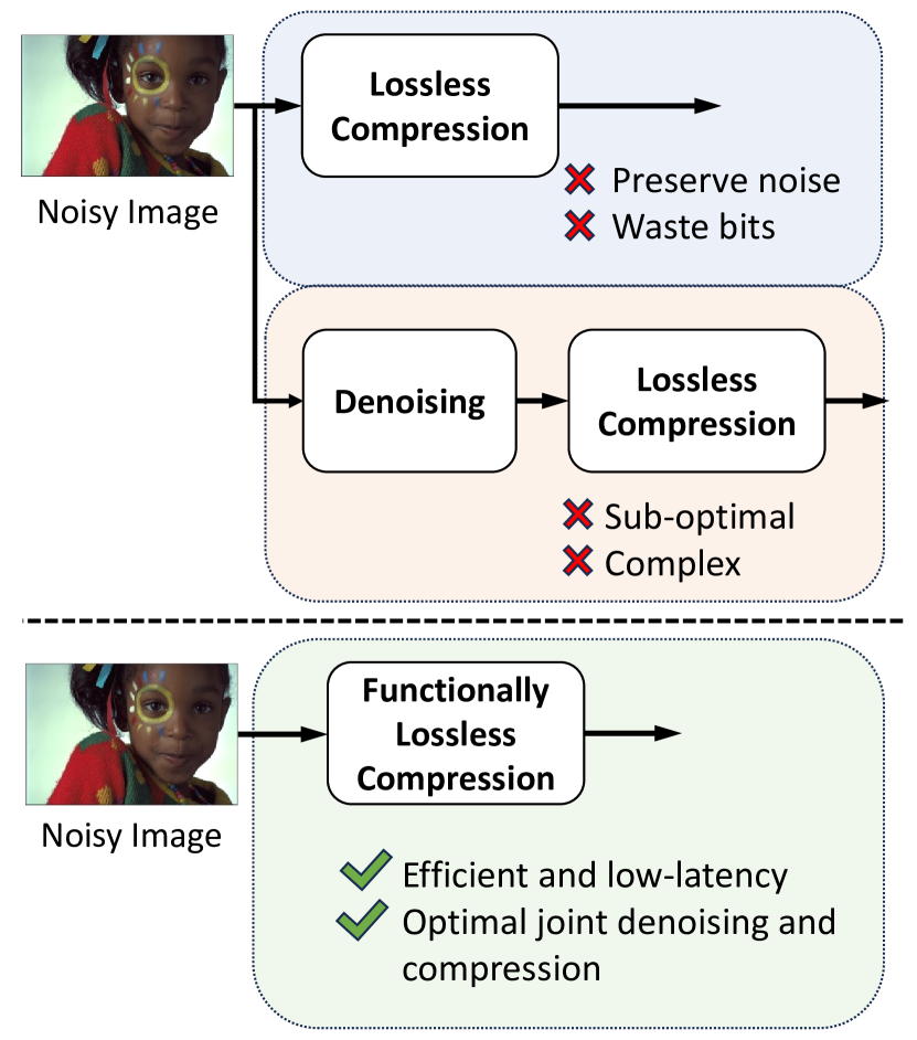
Figure 1: Comparison between the traditional frameworks for lossless compression of noisy images and the proposed functionally lossless compression method.

II Related Works

Image compression [8, 9, 37, 11, 12, 13, 14, 15, 16, 38, 17, 18, 20] and image denoising [39, 40, 41, 42, 43, 44, 45, 46] have been thoroughly studied by researchers in both camps of traditional image processing and modern deep learning. However, the joint image compression and denoising task has been little explored. Very few papers addressed this topic. Testolina et al. [47] investigated the integration of denoising convolutional layers in the decoder of a learning-based compression network. Ranjbar et al. [48] presented a learning-based image compression framework where image denoising and compression are performed jointly. The latent space of the image codec is organized in a scalable manner such that the clean image can be decoded from a subset of the latent space, while the noisy image is decoded from the full latent space at a higher rate. Cheng et al. [49] proposed to optimize the image compression algorithm to be noise-aware as joint denoising and compression. The key is to transform the original noisy images to noise-free bits by eliminating the undesired noise during compression, where the bits are later decompressed as clean images. Huang et al. [50] proposed an efficient end-to-end image compression network, named Noise-Adaptive ResNet VAE (NARV), aiming to handle both clean and noisy input images of different noise levels in a single noise-adaptive compression network without adding nontrivial processing time.

Although these works realized the significance of the joint image compression and denoising problem, they just combined image denoising with lossy compression task, with no regard to the lossless compression problem. To our best knowledge, we are the first to investigate the joint image denoising and lossless compression problem.

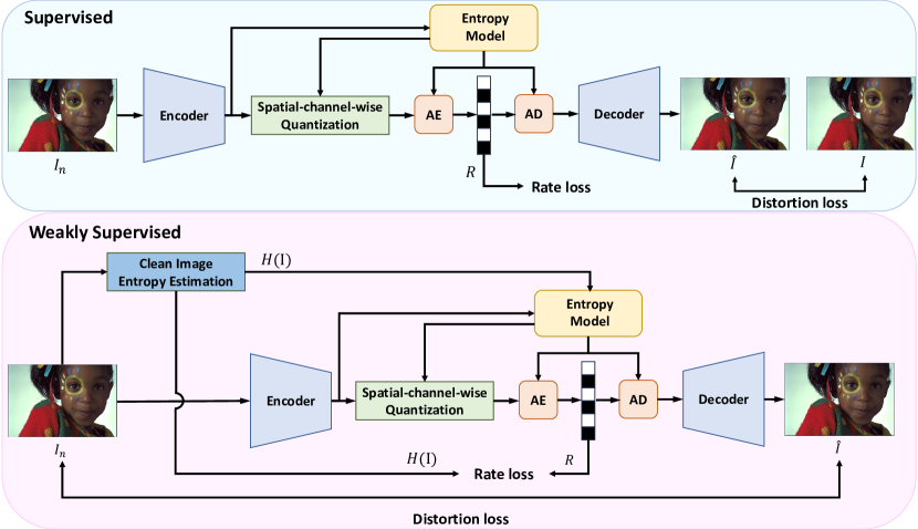
Figure 2: The overall frameworks of the proposed supervised and weakly supervised FLLIC.

III Research Problems and Methodology

III-A Problem formulation

The FLLIC problem can be formulated as follows. Let $I$ be the noise-free latent image, and $I_{n}$ be a noisy observation of $I$, $I_{n}=I+n$. The FLLIC task is to train a neural network to predict an estimate $\hat{I}$ of $I$ that minimizes the distortion, meanwhile minimizing the code length $R(\hat{I})$ of the estimated image $\hat{I}$. We consider two scenarios, the latent clean image $I$ is available and unavailable in the training phase, respectively.

Scenario 1: Supervised joint compression and denoising. If the original clean image $I$ is available in the training phase, the FLLIC will be a supervised learning task and the objective function can be formulated as

$$\centering\text{minimize}\quad||\hat{I}-I||+\lambda\cdot R(\hat{I}).$$ (1)

where $\lambda$ is the Lagrange multiplier. This formulation is very similar to the classical lossy image compression problem, except that the input is a noisy observation and the supervision is the latent noise-free counterpart.

Scenario 2: Weakly supervised joint compression and denoising. In reality, almost all digital sensors inherently introduce acquisition noises, so the strictly noise-free images are unavailable, making the latent clean image $I$ (supervision) absent in the training phase. In order to simplify the problem, we assume that the source entropy $H(I)$ of image $I$ can be obtained. We can use the source entropy $H(I)$ of image $I$ as a weak supervision to guided the network to reconstruct the latent clean image. In this weakly supervised scenario, the objection function can be reformulated as:

$$\centering\text{minimize}\quad||\hat{I}-I_{n}||+\lambda\cdot||R(\hat{I})-H(I)||.$$ (2)

In the objective function, by requiring $\hat{I}$ to be close to $I_{n}$ and $R(\hat{I})$ to approach $H(I)$ at the same time, we make image $\hat{I}$ to be jointly denoised and compressed.

III-B Theoretical analysis of clean entropy estimation

In terms of deep neural networks the FLLIC task is a weakly supervised learning problem. This is because we do not have the clean, uncompressed image $I$ when training the DNN FLLIC model; only the noisy counterpart $I_{n}$ is available in practice. However, the objective function $D(\hat{I})$ has the entropy term $H(I)$. Although it is easy to show $H(I)<H(I_{n})$, estimating $H(I)$ without knowing $I$ itself is a challenge that we need to overcome in this research. We have done some theoretical analysis of $H(I)$ and gained some preliminary understanding. Briefly stating, by modeling the clean image $I$ as a zero-mean Gaussian vector and assume the noisy image $I_{n}$ is obtained by adding a zero-mean Gaussian noise vector $N$ to $I$, the relationship between $H(I_{n})$ and $H(I)$ is given by:

$$H(I_{n})-H(I)=\sum_{i=1}^{n}{\frac{1}{2}log(1+\frac{\sigma_{N}^{2}}{\lambda_{i}})}$$ (3)

where $n$ is the image dimension, $\sigma_{N}^{2}$ is the variance of Gaussian noise and $\lambda_{i}$ is the $i$-th eigenvalue of the covariance matrix of the clean image $I$. The detailed theoretical derivation is as follows.

We model the clean image as a zero-mean Gaussian vector $X$ with covariance matrix $\Sigma_{X}$, and assume that the noisy image $Y$ is obtained by adding to $X$ a zero-mean Gaussian noise vector $N$ with covariance matrix $\Sigma_{N}$. Here $X$ and $N$ have the same dimension $n$ and are independent.

The differential entropies of $X$ and $Y$ are given respectively by

$$h(X)=\frac{1}{2}\text{log}((2\pi e)^{n}\text{det}(\Sigma_{X})),$$ (4)

$$h(Y)=\frac{1}{2}\text{log}((2\pi e)^{n}\text{det}(\Sigma_{X}+\Sigma_{N})).$$

Note that

$$h(Y)-h(X)=\frac{1}{2}\text{log}\frac{\text{det}(\Sigma_{X}+\Sigma_{N})}{det(\Sigma_{X})}>0,$$ (5)

i.e., the differential entropy of the noisy image is greater than that of its clean counterpart.

For simplicity, henceforth we assume $\Sigma_{N}=\sigma^{2}_{N}I$, i.e., the components of $N$ are mutually independent and have the same variance $\sigma^{2}_{N}$. Let $\lambda_{1}\geq\lambda_{2}\geq\cdot\cdot\cdot\geq\lambda_{n}$ be the eigenvalues of $\Sigma_{X}$. Then

$$h(Y)-h(X) =\frac{1}{2}\text{log}\frac{\text{det}(\Sigma_{X}+\sigma_{N}^{2}I)}{det(\Sigma_{X})}$$ (6)

$$=\sum_{i=1}^{n}\frac{1}{2}\text{log}(1+\frac{\sigma_{N}^{2}}{\lambda_{i}}).$$

If $\sigma_{N}^{2}$ is much smaller than $\lambda_{n}$, we have

$$\sum_{i=1}^{n}\frac{1}{2}\text{log}(1+\frac{\sigma_{N}^{2}}{\lambda_{i}})\approx\sum_{i=1}^{n}\frac{\sigma_{N}^{2}}{2\lambda_{i}}.$$ (7)

In practice, Fourier coefficients can be used as the substitute of eigenvalues.

Actually, it is more appropriate to model the clean image and its noisy counterpart respectively as $X^{\Delta}$ and $Y^{\Delta}$, which are obtained from $X$ and $Y$ by quantizing each component using a scalar quantizer of step size $\Delta$. It can be shown that when $\Delta$ is sufficiently small,

$$H(X^{\Delta})\approx h(X)-n\text{log}\Delta,$$ (8)

$$H(Y^{\Delta})\approx h(Y)-n\text{log}\Delta,$$

which implies

$$h(Y)-h(X)=H(Y^{\Delta})-H(X^{\Delta}).$$ (9)

III-C Practical estimation of clean image entropy

In pursue of practical solutions to the MLLIC problem, we explore and realize the potential of DNNs in learning $H(I)$ from $I_{n}$ (the noisy observation of $I$), $H(I_{n})$ (estimated by losslessly compressing $I_{n}$ with a DNN MLLIC model), and the probability model of the noise $N$ (if available).

Specifically, we design a deep neural network which takes $I_{n}$, $H(I_{n})$ and $\sigma_{N}$ (variance of the noise) as input to estimate the source entropy of the clean image $H(I)$. The network framework is shown in Fig. 3. It consists of two components, feature extraction module and regression module. For feature extraction module, an auto-encoder network is adopted as the backbone network to extract high-dimension nonlinear features $F(I_{n})$ from the noisy observations $I_{n}$. Next the extracted features $F(I_{n})$ is combined with $H(I_{n})$ and $\sigma_{N}$, and then fed into the regression module to predict the estimated $H(I)$. The regression module is built up with two fully-connected layers.

The auto-encoder used for feature extraction is a U-Net-like Encoder-Decoder network. The encoder part has an input convolution layer and five stages comprised of a max-pooling layer followed by two convolutional layers. The input layer has 32 convolution filters with size of 3$\times$3 and stride of 1. The first stage is size-invariant and the other four stages gradually reduce the feature map resolution by max-pooling to obtain a larger receptive field. The decoder is almost symmetrical to the encoder. Each stage consists of a bilinear upsampling layer followed by two convolution layers and a ReLU activation function. The input of each layer is the concatenated feature maps of the up-sampled output from its previous layer and its corresponding layer in the encoder.

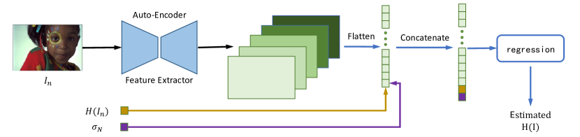
Figure 3: The overall architecture of the neural network for estimating the source entropy of clean image from its noisy observation.

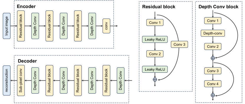
Figure 4: The detailed architectures of the encoder and decoder networks in FLLIC.

III-D Network design

The overall frameworks of the proposed supervised and weakly supervised FLLIC are illustrated in Fig. 2.

For the supervised FLLIC problem, given the noisy image $I_{n}$, we firstly encode the noisy image to the latent space for feature extraction. Then we obtain the content adaptive quantization intervals from the entropy model and apply the spatial-channel-wise quantization on the latent features. The quantized features are fed into entropy model for conditional probability estimation and for further arithmetic coding. In the decoder, the arithmetic decoded codes are fed into a decoder for noise-free image reconstruction. We minimize the distortion between the reconstructed image and the supervised clean image.

For the weakly supervised FLLIC problem, given the noisy image $I_{n}$, we estimate the entropy of clean image $\hat{H(I)}$ and use it to guide the entropy model to predict the spatial-channel-wise quantization intervals for the encoded latent features. Due to the lack of supervised clean image, we utilize the noisy image $I_{n}$ itself as the supervised image and minimize the distortion between the reconstructed image and the noisy image. We also hope that the rate of quantized latent features approaches the entropy of latent noise-free clean image.

To achieve better quantization performance, we adopt the learnable content-adaptive quantization technique, which is firstly introduced in [51, 52], to perform adaptive quantization for different contents. Specifically, for each input image, we learn different quantization steps for each position and channel. The spatial-channel-wise quantization steps are generated by the entropy model, dynamically changing to adapt different image contents and noise intensity. Such design helps us improve the final reconstruction and coding performance by content-adaptive bit allocation. Intuitively, positions with larger noise intensity will be allocated with larger quantization steps.

Following [52], we adopt residual convolution blocks and depth-wise convolution blocks to build the encoder and decoder network for low-latency requirement, instead of using Transformer as recent SOTA model [53, 54, 20]. Fig. 4 presents the detailed structures of the encoder and decoder networks. In the encoder network, it contains three residual blocks and three depth convolution blocks. Each residual block consists of two convolution layers and two Leaky ReLU layers with s skip-connected convolution layer. Each depth convolution block contains four convolution layers and one depth convolution layer with two cascaded skip connections. In the decoder network, it contains four depth convolution block and three residual blocks, almost the mirror of the encoder network.

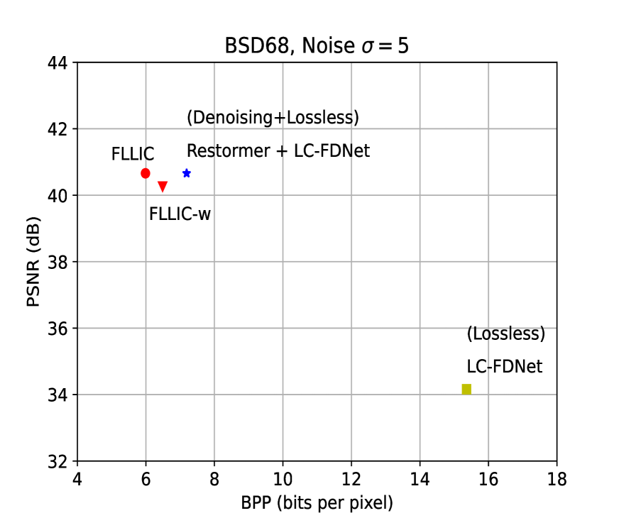
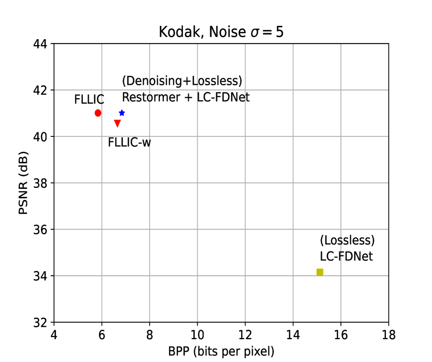
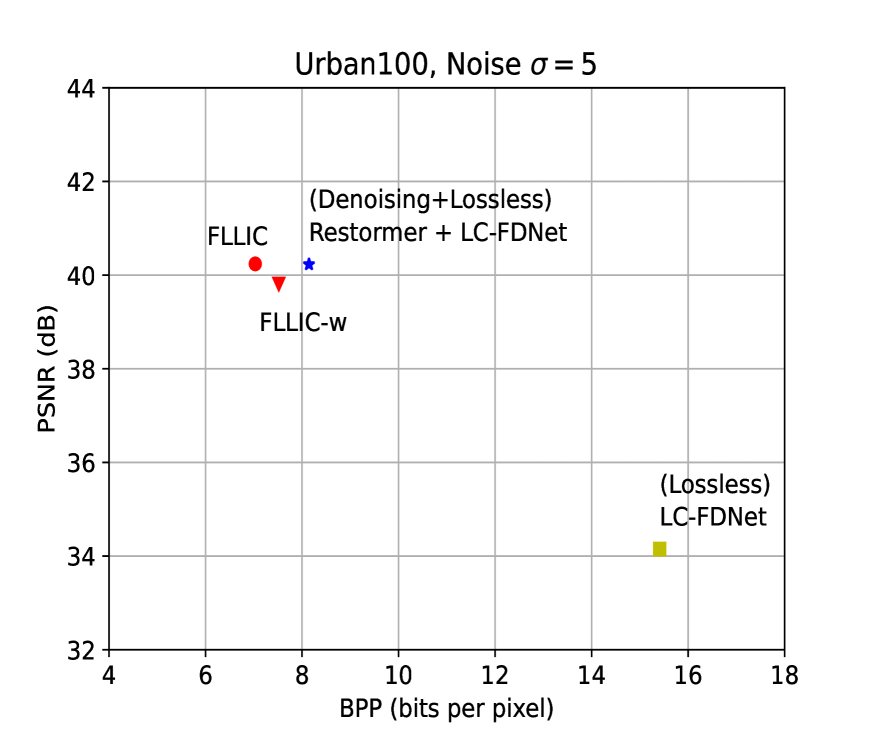
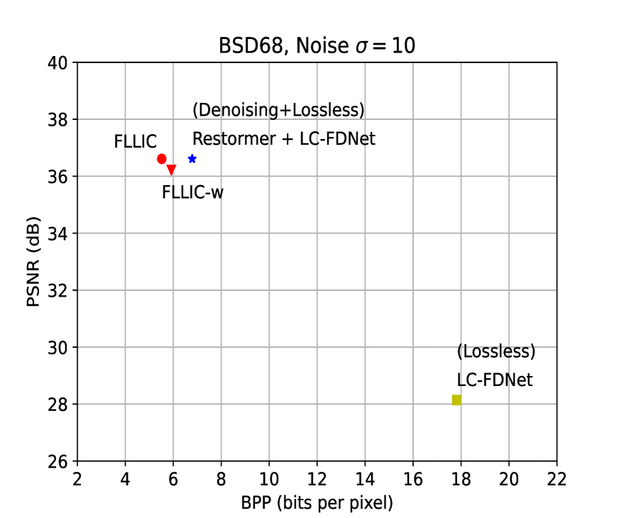
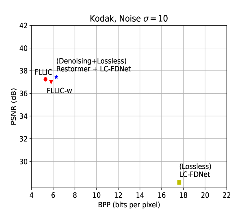
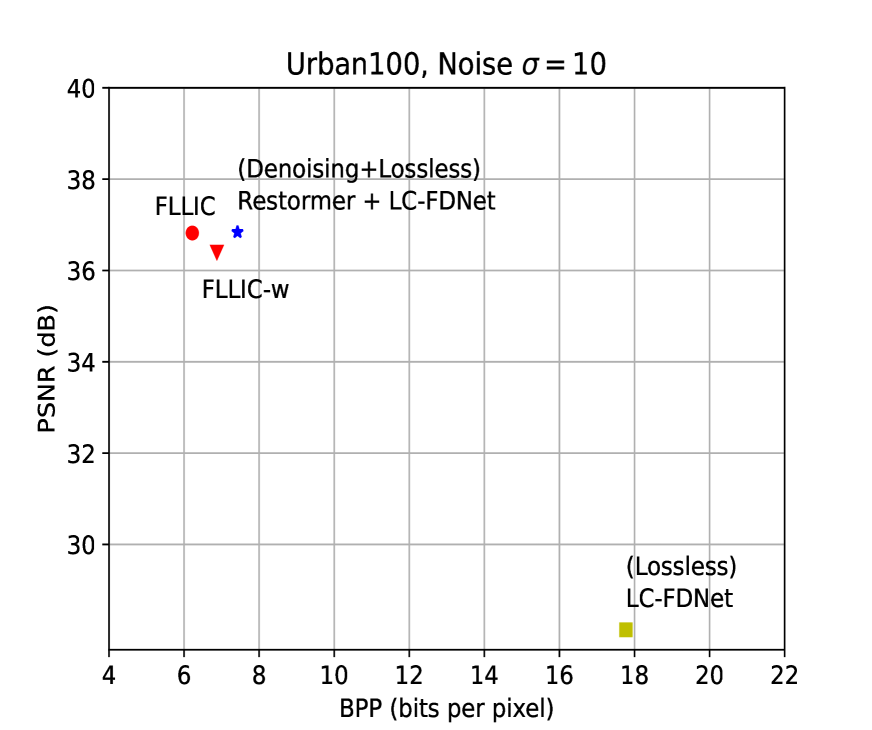
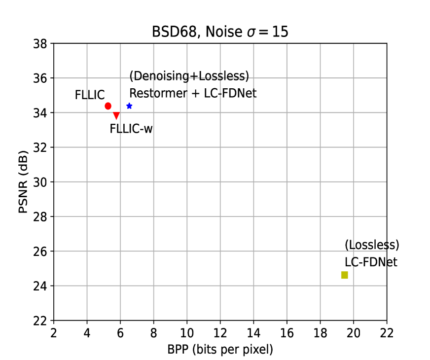
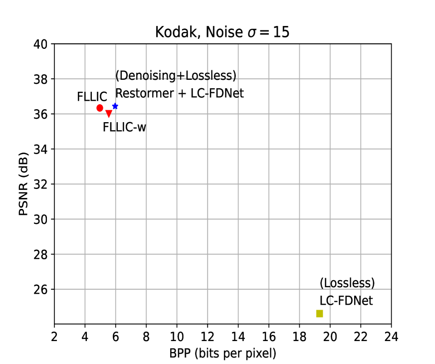
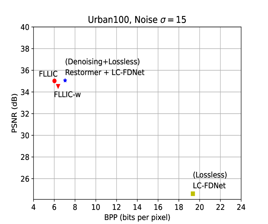
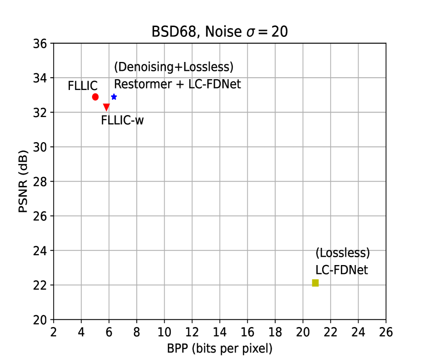
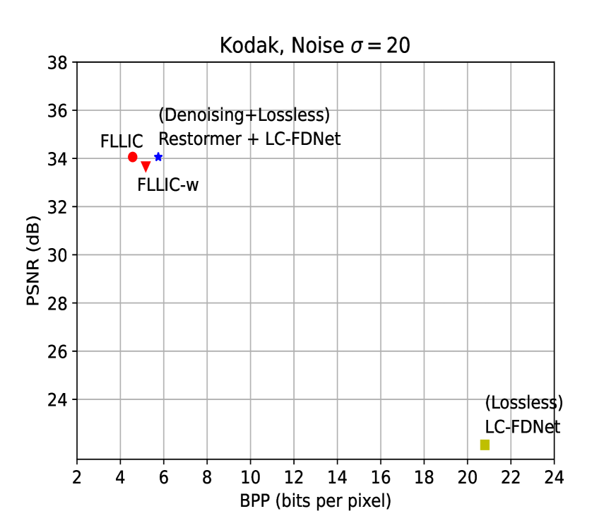
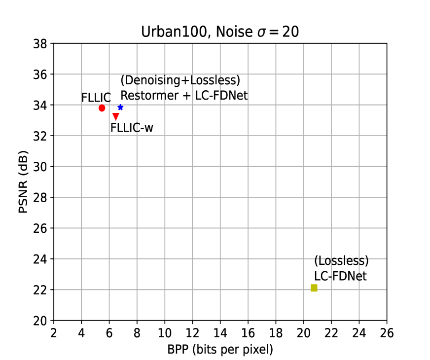
Figure 5: Quantitative results on the various combinations of different synthetic datasets (BSD600, Kodak24, Urban100) and different noise intensities ($\sigma$=5,10,15,20). ”FLLIC” represents the supervised FLLIC and ’FLLIC-w’ represents the weakly-supervised FLLIC.

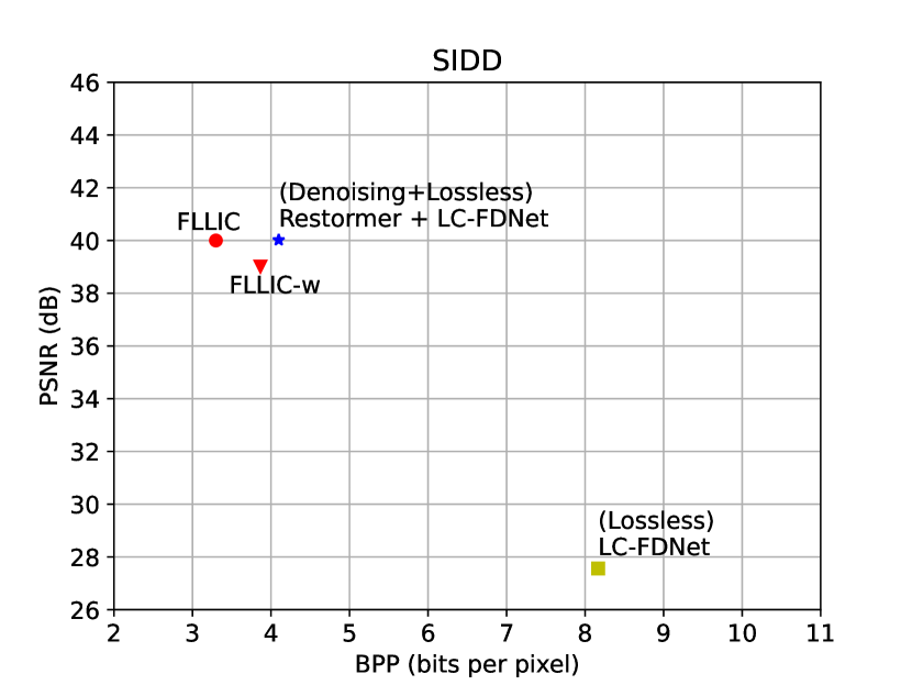
Figure 6: Quantitative results on the real world dataset SIDD. ”FLLIC” represents the supervised FLLIC and ’FLLIC-w’ represents the weakly-supervised FLLIC.

IV Experiments

In this section, we present the implementation details of the proposed FLLIC compression system. To systematically evaluate and analyze the performance of the FLLIC compression system, we conduct extensive experiments and compare our results with several stat-of-the-art methods on quantitative metric and inference complexity.

IV-A Experiment setup

In this part, we describe the experiment setup including the following four aspects: dataset preparation, training details, baselines and metrics.

Datasets. Following the previous work on lossless image compression [55], we train the proposed network with Flickr2k dataset [56], which contains 2,000 high-quality images. We evaluate the trained network on three synthetic benchmark datasets generated with additive white Gaussian noise (BSD68 [57], Urban100 [58] and Kodak24 [59]). Unlike the pure image denoising task which utilizes very large noise level, we include four relatively small noise levels: $\sigma=5,10,15,20$. We also evaluate the proposed FLLIC compression method on a real-world dataset SIDD [60], which contains  30,000 noisy images from 10 scenes under different lighting conditions using five representative smartphone cameras and the corresponding generated ’noise-free’ clean images.

Training details. During training, we randomly extract patches of size $256\times 256$. All training processes use the Adam [61] optimizer by setting $\beta_{1}=0.9$ and $\beta_{2}=0.999$, with a batch size of $128$. The learning rate starts from $1\times 10^{-4}$ and decays by a factor of 0.5 every $4\times 10^{4}$ iterations and finally ends with $1.25\times 10^{-5}$. We train our model with PyTorch on a NVIDIA RTX 4090 GPU. It takes about two days to converge. Before training the FLLIC network, we first train the clean entropy network in Fig. 3 by DIV2K [62] dataset. The training strategy is the same as above.

For the synthetic denoising dataset, we train a specific network for each noise level. In other words, we select a optimal Lagrange multiplier $\lambda$ for each noise level. The details of $\lambda$ selection are provided in the supplementary material.

Baselines. To show the superiority of the proposed FLLIC compression method over pure lossless image compression and the cascaded approach of denoising + lossless compression, we build two competing baselines with the state-of-the-art methods in denoising (Restormer [46]) and lossless image compression (LC-FDNet [55]), respectively.
Baseline 1. Pure lossless compression using LC-FDNet.
Baseline 2. Cascaded approach of Restormer + LC-FDNet.
Restormer [46] is the state-of-the-art image restortion network, which built upon the popular transformer architecture. It achieves the best results on various image restoration tasks, such as image deblurring, deraining and denoising. LC-FDNEt [55] is the state-of-the-art open-sourced lossless image compression method, which proceeds the encoding in a coarse-to-fine manner to separate and process low and high-frequency regions differently. To do a fair comparison and make the baselines more robust to the noisy/denoised images, we finetune the cascaded baseline using Flickr2K dataset. The open-accessed pre-trained weights of each method are adopted as the initialization of the finetuning.

Metrics. We use rate-distortion (BPP-PSNR) metric to measure the compression performance of the proposed FLLIC compression method. In the ideal lossless compression, as the reconstruction is equivalent to the original image, therefore there is no distortion term. However, in the FLLIC framework, the reconstructed image is compared to the latent noise-free image, so it is necessary to compare the distortion term.

IV-B Quantitative results

Fig. 5 provides the comparison of quantitative results on the synthetic benchmark datasets. It can be seen that our proposed FLLIC achieves the highest reconstruction quality (PSNR) and also the lowest bit rate (BPP). It shows that pure lossless image compression achieves the highest BPP and the lowest PSNR, which implies that directly applying lossless image compression on noisy image is inefficient. We can also find that the cascaded method of denoising and lossless compression is still inferior to the proposed FLLIC framework. Specifically, the supervised FLLIC achieves the competing psnr as the cascaded approach while being near 1 bpp smaller than the latter in terms of bit rate. The weakly supervised FLLIC is slightly inferior to the supervised FLLIC in terms of performance, but considering that this scheme is trained without supervised clean images, it is amazing to achieve such results. Fig. 6 shows the compression performance of competing methods on the real world dataset SIDD. We can see that the proposed FLLIC compression method achieves the bset rate-distortion performance in the real-world dataset, which suggests that the proposed FLLIC can be used in real scenarios.

IV-C Inference time

We measure the inference time required for encoding and decoding a $512\times 512$ image on a Nvidia RTX 4090 GPU. The detailed inference time of competing methods are listed in Table I. For the cascaded method, encoding an images needs two steps: denoising and lossless compression, which need about 400 ms per step by the state-of-the-art algorithms. However, the proposed FLLIC just needs about 60 ms by one pass, which is an order of magnitude lower than the Restormer and LC-FDNet. Considering that FLLIC achieves better rate-distortion performance than the cascade scheme, it is amazing that it is also substantially ahead in inference time.

TABLE I: Inference time (ms) of cascaded method of denoising + lossless compression and the proposed FLLIC method for encoding and decoding a $512\times 512$ image on a Nvidia RTX 4090 GPU.

	Cascaded
	Restormer	LC-FDNet	FLLIC
Encoding	465 ms	428 ms	65.8 ms
Decoding	-	462 ms	62.1 ms

IV-D Ablation studies

In this subsection, we test various ablations of our full architecture to evaluate the effects of each component of the proposed FLLIC compression system.

Firstly, we systematically assess the impact of content adaptive quantization. To delve deeper into this evaluation, we construct a purposeful ablation architecture, denoted as FLLIC-u, wherein uniform quantization is employed instead of content adaptive quantization. Subsequently, we meticulously analyze the influence of incorporating guidance from the clean image entropy. This involves the removal of the branch associated with clean image entropy from the weakly supervised FLLIC network, with subsequent reporting of the resultant compression performance. The architecture without the guidance of the clean image entropy is denoted as FLLIC-w0.

The results of the analyses on these two ablation architectures are depicted in Fig. 7. Firstly, it is evident that the elimination of the content adaptive quantization module leads to a notable decline in compression performance (PSNR decreases by approximately 0.8dB, and the rate increases by about 0.5bpp). Furthermore, a significant observation is the substantial positive impact of incorporating guidance from the clean image entropy on the compression performance of FLLIC. Removal of the clean image entropy guidance results in a noteworthy reduction in PSNR by around 1.5dB, and an increase in rate by approximately 0.5bpp. These changes are particularly significant in the realm of compression.

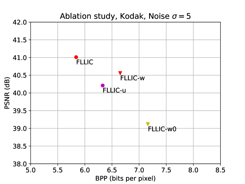
Figure 7: Ablation results on the Kodak dataset with Gaussian noise of $\sigma$=5. ”FLLIC” represents the supervised FLLIC and ’FLLIC-w’ represents the weakly-supervised FLLIC. ”FLLIC-u” represents the FLLIC compression method with uniform quantization. ’FLLIC-w0’ represents the weakly supervised FLLIC compression network without the guidance of clean image entropy.

IV-E Limitation

The main limitation of this work is its need to train a specific network for a given noise level. The current version hardly generalizes to various noise levels by a single network. A possible solution could be estimating noise level first and using the estimated noise level as known a prior for the encoding and decoding. We leave detailed study of this limitation to the further work.

V Conclusion

We introduce a new paradigm called functionally lossless image compression (FLLIC), which integrates the two tasks of denoising and compression. FLLIC engages in lossless/near-lossless compression of optimally denoised images, with optimality tailored to specific tasks. While not strictly adhering to the literal meaning of losslessness concerning the noisy input, FLLIC aspires to achieve the optimal reconstruction of the latent noise-free original image. Extensive empirical investigations underscore the state-of-the-art performance of FLLIC in the realm of joint denoising and compression for noisy images, concurrently exhibiting advantages in terms of computational efficiency and cost-effectiveness.

Xi Zhang received the B.Sc. degree in mathematics and physics basic science from University of Electronic Science and Technology of China, in 2015, and the Ph.D. degree in electronic engineering from Shanghai Jiao Tong University, China, in 2022. He was also a visiting Ph.D. student with the Department of Electrical and Computer Engineering, McMaster University, Hamilton, ON, Canada. He is currently a Postdoctoral Fellow with the Department of Electronic Engineering, Shanghai Jiao Tong University, China. His research interests include image and video processing, especially in image and video compression, enhancement, etc. He is also interested in other deep learning tasks such as domain generalization and visual reasoning.

Xiaolin Wu (Fellow, IEEE) received the B.Sc. degree in computer science from Wuhan University, China, in 1982, and the Ph.D. degree in computer science from the University of Calgary, Canada, in 1988. He started his academic career in 1988. He was a Faculty Member with Western University, Canada, and New York Polytechnic University (NYU-Poly), USA. He is currently with McMaster University, Canada, where he is a Distinguished Engineering Professor and holds an NSERC Senior Industrial Research Chair. His research interests include image processing, data compression, digital multimedia, low-level vision, and network-aware visual communication. He has authored or coauthored more than 300 research articles and holds four patents in these fields. He served on technical committees of many IEEE international conferences/workshops on image processing, multimedia, data compression, and information theory. He was a past Associated Editor of IEEE TRANSACTIONS ON MULTIMEDIA. He is also an Associated Editor of IEEE TRANSACTIONS ON IMAGE PROCESSING.

References

- [1] J. Ballé, V. Laparra, and E. P. Simoncelli, “End-to-end optimized image compression,” in 5th International Conference on Learning Representations, ICLR, 2017.
- [2] L. Theis, W. Shi, A. Cunningham, and F. Huszár, “Lossy image compression with compressive autoencoders,” in 5th International Conference on Learning Representations, ICLR, 2017.
- [3] E. Agustsson, F. Mentzer, M. Tschannen, L. Cavigelli, R. Timofte, L. Benini, and L. V. Gool, “Soft-to-hard vector quantization for end-to-end learning compressible representations,” in Advances in Neural Information Processing Systems 30, 2017, pp. 1141–1151.
- [4] J. Ballé, D. Minnen, S. Singh, S. J. Hwang, and N. Johnston, “Variational image compression with a scale hyperprior,” in 6th International Conference on Learning Representations, ICLR. OpenReview.net, 2018.
- [5] D. Minnen, J. Ballé, and G. Toderici, “Joint autoregressive and hierarchical priors for learned image compression,” in Advances in Neural Information Processing Systems 31, 2018, pp. 10 794–10 803.
- [6] F. Mentzer, E. Agustsson, M. Tschannen, R. Timofte, and L. V. Gool, “Conditional probability models for deep image compression,” in 2018 IEEE Conference on Computer Vision and Pattern Recognition, CVPR, 2018, pp. 4394–4402.
- [7] J. Lee, S. Cho, and S. Beack, “Context-adaptive entropy model for end-to-end optimized image compression,” in 7th International Conference on Learning Representations, ICLR, 2019.
- [8] Z. Cheng, H. Sun, M. Takeuchi, and J. Katto, “Learned image compression with discretized gaussian mixture likelihoods and attention modules,” in 2020 IEEE/CVF Conference on Computer Vision and Pattern Recognition, CVPR, 2020, pp. 7936–7945.
- [9] F. Mentzer, G. D. Toderici, M. Tschannen, and E. Agustsson, “High-fidelity generative image compression,” Advances in Neural Information Processing Systems, vol. 33, pp. 11 913–11 924, 2020.
- [10] X. Zhang and X. Wu, “Attention-guided image compression by deep reconstruction of compressive sensed saliency skeleton,” in Proceedings of the IEEE/CVF Conference on Computer Vision and Pattern Recognition, 2021, pp. 13 354–13 364.
- [11] D. He, Y. Zheng, B. Sun, Y. Wang, and H. Qin, “Checkerboard context model for efficient learned image compression,” in Proceedings of the IEEE/CVF Conference on Computer Vision and Pattern Recognition (CVPR), June 2021, pp. 14 771–14 780.
- [12] F. Yang, L. Herranz, Y. Cheng, and M. G. Mozerov, “Slimmable compressive autoencoders for practical neural image compression,” in Proceedings of the IEEE/CVF Conference on Computer Vision and Pattern Recognition (CVPR), June 2021, pp. 4998–5007.
- [13] J.-H. Kim, B. Heo, and J.-S. Lee, “Joint global and local hierarchical priors for learned image compression,” in Proceedings of the IEEE/CVF Conference on Computer Vision and Pattern Recognition, 2022, pp. 5992–6001.
- [14] D. He, Z. Yang, W. Peng, R. Ma, H. Qin, and Y. Wang, “Elic: Efficient learned image compression with unevenly grouped space-channel contextual adaptive coding,” in Proceedings of the IEEE/CVF Conference on Computer Vision and Pattern Recognition, 2022, pp. 5718–5727.
- [15] C. Gao, T. Xu, D. He, Y. Wang, and H. Qin, “Flexible neural image compression via code editing,” Advances in Neural Information Processing Systems, vol. 35, pp. 12 184–12 196, 2022.
- [16] T. Xu, Y. Wang, D. He, C. Gao, H. Gao, K. Liu, and H. Qin, “Multi-sample training for neural image compression,” arXiv preprint arXiv:2209.13834, 2022.
- [17] J. Lee, S. Jeong, and M. Kim, “Selective compression learning of latent representations for variable-rate image compression,” arXiv preprint arXiv:2211.04104, 2022.
- [18] C. Shin, H. Lee, H. Son, S. Lee, D. Lee, and S. Lee, “Expanded adaptive scaling normalization for end to end image compression,” in European Conference on Computer Vision. Springer, 2022, pp. 390–405.
- [19] X. Zhang and X. Wu, “Dual-layer image compression via adaptive downsampling and spatially varying upconversion,” arXiv preprint arXiv:2302.06096, 2023.
- [20] R. Zou, C. Song, and Z. Zhang, “The devil is in the details: Window-based attention for image compression,” in Proceedings of the IEEE/CVF conference on computer vision and pattern recognition, 2022, pp. 17 492–17 501.
- [21] X. Zhang and X. Wu, “Lvqac: Lattice vector quantization coupled with spatially adaptive companding for efficient learned image compression,” in Proceedings of the IEEE/CVF Conference on Computer Vision and Pattern Recognition, 2023, pp. 10 239–10 248.
- [22] F. Mentzer, E. Agustsson, M. Tschannen, R. Timofte, and L. V. Gool, “Practical full resolution learned lossless image compression,” in Proceedings of the IEEE/CVF conference on computer vision and pattern recognition, 2019, pp. 10 629–10 638.
- [23] F. Mentzer, L. V. Gool, and M. Tschannen, “Learning better lossless compression using lossy compression,” in Proceedings of the IEEE/CVF Conference on Computer Vision and Pattern Recognition, 2020, pp. 6638–6647.
- [24] X. Zhang and X. Wu, “Nonlinear prediction of multidimensional signals via deep regression with applications to image coding,” in ICASSP 2019-2019 IEEE International Conference on Acoustics, Speech and Signal Processing (ICASSP). IEEE, 2019, pp. 1602–1606.
- [25] F. Kingma, P. Abbeel, and J. Ho, “Bit-swap: Recursive bits-back coding for lossless compression with hierarchical latent variables,” in International Conference on Machine Learning. PMLR, 2019, pp. 3408–3417.
- [26] J. Townsend, T. Bird, J. Kunze, and D. Barber, “Hilloc: Lossless image compression with hierarchical latent variable models,” arXiv preprint arXiv:1912.09953, 2019.
- [27] E. Hoogeboom, J. Peters, R. Van Den Berg, and M. Welling, “Integer discrete flows and lossless compression,” Advances in Neural Information Processing Systems, vol. 32, 2019.
- [28] J. Ho, E. Lohn, and P. Abbeel, “Compression with flows via local bits-back coding,” Advances in Neural Information Processing Systems, vol. 32, 2019.
- [29] X. Zhang and X. Wu, “Ultra high fidelity deep image decompression with -constrained compression,” IEEE Transactions on Image Processing, vol. 30, pp. 963–975, 2020.
- [30] S. Zhang, N. Kang, T. Ryder, and Z. Li, “iflow: Numerically invertible flows for efficient lossless compression via a uniform coder,” Advances in Neural Information Processing Systems, vol. 34, pp. 5822–5833, 2021.
- [31] S. Zhang, C. Zhang, N. Kang, and Z. Li, “ivpf: Numerical invertible volume preserving flow for efficient lossless compression,” in Proceedings of the IEEE/CVF Conference on Computer Vision and Pattern Recognition, 2021, pp. 620–629.
- [32] N. Kang, S. Qiu, S. Zhang, Z. Li, and S.-T. Xia, “Pilc: Practical image lossless compression with an end-to-end gpu oriented neural framework,” in Proceedings of the IEEE/CVF Conference on Computer Vision and Pattern Recognition, 2022, pp. 3739–3748.
- [33] A. Van Den Oord, N. Kalchbrenner, and K. Kavukcuoglu, “Pixel recurrent neural networks,” in International conference on machine learning. PMLR, 2016, pp. 1747–1756.
- [34] T. Salimans, A. Karpathy, X. Chen, and D. P. Kingma, “Pixelcnn++: Improving the pixelcnn with discretized logistic mixture likelihood and other modifications,” arXiv preprint arXiv:1701.05517, 2017.
- [35] D. P. Kingma and M. Welling, “Auto-encoding variational bayes,” arXiv preprint arXiv:1312.6114, 2013.
- [36] I. Kobyzev, S. J. Prince, and M. A. Brubaker, “Normalizing flows: An introduction and review of current methods,” IEEE transactions on pattern analysis and machine intelligence, vol. 43, no. 11, pp. 3964–3979, 2020.
- [37] X. Zhang, X. Wu, X. Zhai, X. Ben, and C. Tu, “Davd-net: Deep audio-aided video decompression of talking heads,” in Proceedings of the IEEE/CVF Conference on Computer Vision and Pattern Recognition, 2020, pp. 12 335–12 344.
- [38] X. Zhang and X. Wu, “Multi-modality deep restoration of extremely compressed face videos,” IEEE Transactions on Pattern Analysis and Machine Intelligence, vol. 45, no. 2, pp. 2024–2037, 2022.
- [39] K. Zhang, W. Zuo, Y. Chen, D. Meng, and L. Zhang, “Beyond a gaussian denoiser: Residual learning of deep cnn for image denoising,” IEEE transactions on image processing, vol. 26, no. 7, pp. 3142–3155, 2017.
- [40] D. Ulyanov, A. Vedaldi, and V. Lempitsky, “Deep image prior,” in Proceedings of the IEEE conference on computer vision and pattern recognition, 2018, pp. 9446–9454.
- [41] T. Huang, S. Li, X. Jia, H. Lu, and J. Liu, “Neighbor2neighbor: Self-supervised denoising from single noisy images,” in Proceedings of the IEEE/CVF conference on computer vision and pattern recognition, 2021, pp. 14 781–14 790.
- [42] J. Liang, J. Cao, G. Sun, K. Zhang, L. Van Gool, and R. Timofte, “Swinir: Image restoration using swin transformer,” in Proceedings of the IEEE/CVF international conference on computer vision, 2021, pp. 1833–1844.
- [43] Y. Zhao, Z. Jiang, A. Men, and G. Ju, “Pyramid real image denoising network,” in 2019 IEEE Visual Communications and Image Processing (VCIP). IEEE, 2019, pp. 1–4.
- [44] S. Guo, Z. Yan, K. Zhang, W. Zuo, and L. Zhang, “Toward convolutional blind denoising of real photographs,” in Proceedings of the IEEE/CVF conference on computer vision and pattern recognition, 2019, pp. 1712–1722.
- [45] C. Ren, X. He, C. Wang, and Z. Zhao, “Adaptive consistency prior based deep network for image denoising,” in Proceedings of the IEEE/CVF conference on computer vision and pattern recognition, 2021, pp. 8596–8606.
- [46] S. W. Zamir, A. Arora, S. Khan, M. Hayat, F. S. Khan, and M.-H. Yang, “Restormer: Efficient transformer for high-resolution image restoration,” in Proceedings of the IEEE/CVF conference on computer vision and pattern recognition, 2022, pp. 5728–5739.
- [47] M. Testolina, E. Upenik, and T. Ebrahimi, “Towards image denoising in the latent space of learning-based compression,” in Applications of Digital Image Processing XLIV, vol. 11842. SPIE, 2021, pp. 412–422.
- [48] S. Ranjbar Alvar, M. Ulhaq, H. Choi, and I. V. Bajić, “Joint image compression and denoising via latent-space scalability,” Frontiers in Signal Processing, vol. 2, p. 932873, 2022.
- [49] K. L. Cheng, Y. Xie, and Q. Chen, “Optimizing image compression via joint learning with denoising,” in European Conference on Computer Vision. Springer, 2022, pp. 56–73.
- [50] Y. Huang, Z. Duan, and F. Zhu, “Narv: An efficient noise-adaptive resnet vae for joint image compression and denoising,” in 2023 IEEE International Conference on Multimedia and Expo Workshops (ICMEW). IEEE, 2023, pp. 188–193.
- [51] J. Li, B. Li, and Y. Lu, “Hybrid spatial-temporal entropy modelling for neural video compression,” in Proceedings of the 30th ACM International Conference on Multimedia, 2022, pp. 1503–1511.
- [52] G.-H. Wang, J. Li, B. Li, and Y. Lu, “Evc: Towards real-time neural image compression with mask decay,” arXiv preprint arXiv:2302.05071, 2023.
- [53] Y. Zhu, Y. Yang, and T. Cohen, “Transformer-based transform coding,” in International Conference on Learning Representations, 2022.
- [54] Y. Qian, M. Lin, X. Sun, Z. Tan, and R. Jin, “Entroformer: A transformer-based entropy model for learned image compression,” in International Conference on Learning Representations, 2022.
- [55] H. Rhee, Y. I. Jang, S. Kim, and N. I. Cho, “Lc-fdnet: Learned lossless image compression with frequency decomposition network,” in Proceedings of the IEEE/CVF Conference on Computer Vision and Pattern Recognition, 2022, pp. 6033–6042.
- [56] B. Lim, S. Son, H. Kim, S. Nah, and K. Mu Lee, “Enhanced deep residual networks for single image super-resolution,” in Proceedings of the IEEE conference on computer vision and pattern recognition workshops, 2017, pp. 136–144.
- [57] D. Martin, C. Fowlkes, D. Tal, and J. Malik, “A database of human segmented natural images and its application to evaluating segmentation algorithms and measuring ecological statistics,” in Proceedings Eighth IEEE International Conference on Computer Vision. ICCV 2001, vol. 2. IEEE, 2001, pp. 416–423.
- [58] J.-B. Huang, A. Singh, and N. Ahuja, “Single image super-resolution from transformed self-exemplars,” in Proceedings of the IEEE conference on computer vision and pattern recognition, 2015, pp. 5197–5206.
- [59] R. Franzen, “Kodak lossless true color image suite,” 1999, http://r0k.us/graphics/kodak/.
- [60] A. Abdelhamed, S. Lin, and M. S. Brown, “A high-quality denoising dataset for smartphone cameras,” in Proceedings of the IEEE conference on computer vision and pattern recognition, 2018, pp. 1692–1700.
- [61] D. P. Kingma and J. Ba, “Adam: A method for stochastic optimization,” arXiv preprint arXiv:1412.6980, 2014.
- [62] E. Agustsson and R. Timofte, “Ntire 2017 challenge on single image super-resolution: Dataset and study,” in The IEEE Conference on Computer Vision and Pattern Recognition (CVPR) Workshops, July 2017.