Revisiting the warm sub-Saturn TOI-1710b

The Transiting Exoplanet Survey Satellite (TESS) provides a continuous suite of new planet candidates that need confirmation and precise mass determination from ground-based observatories. This is the case for the G-type star TOI-1710, which is known to host a transiting sub-Saturn planet ($\mathrm{M_{p}}$ $=$ 28.3 $\pm$ 4.7 $\mathrm{M}_{\oplus}$) in a long-period orbit ($P$ = 24.28 d). Here we combine archival SOPHIE and new and archival HARPS-N radial velocity data with newly available TESS data to refine the planetary parameters of the system and derive a new mass measurement for the transiting planet, taking into account the impact of the stellar activity on the mass measurement. We report for TOI-1710 b a radius of $\mathrm{R_{p}}$ $=$ 5.15 $\pm$ 0.12 $\mathrm{R}_{\oplus}$, a mass of $\mathrm{M_{p}}$ $=$ 18.4 $\pm$ 4.5 $\mathrm{M}_{\oplus}$, and a mean bulk density of $\rho_{\rm p}$ $=$ 0.73 $\pm$ 0.18 $\mathrm{g\,cm^{-3}}$, which are consistent at 1.2$\sigma$, 1.5$\sigma$, and 0.7$\sigma$, respectively, with previous measurements. Although there is not a significant difference in the final mass measurement, we needed to add a Gaussian process component to successfully fit the radial velocity dataset. This work illustrates that adding more measurements does not necessarily imply a better mass determination in terms of precision, even though they contribute to increasing our full understanding of the system. Furthermore, TOI-1710 b joins an intriguing class of planets with radii in the range 4–8 $\mathrm{R}_{\oplus}$ that have no counterparts in the Solar System. A large gaseous envelope and a bright host star make TOI-1710 b a very suitable candidate for follow-up atmospheric characterization.

1 Introduction

The Transiting Exoplanet Survey Satellite (TESS; Ricker et al., 2015) is a NASA-sponsored space telescope launched on April 18, 2018. The original TESS mission was a two-year full-sky survey to search for transiting planets, but the mission obtained a first extension of observations covering from July 2020 to September 2022. TESS is currently in its second extended mission, which will last at least until September 2025. One of the TESS mission’s main goals is to look for 50 small planets with $\mathrm{R_{P}}$¡4 $\mathrm{R}_{\oplus}$ suitable for atmospheric characterization. However, during that search TESS has detected planets with a wide range of radii. In particular, TOI-216b (Dawson et al., 2021), TOI-421c (Carleo et al., 2020), TOI-674b (Murgas et al., 2021), LTT 9779b (Jenkins et al., 2020), and TOI-257b (Addison et al., 2021) are some examples of confirmed planets alerted by TESS that have sizes between Uranus (4 $\mathrm{R}_{\oplus}$) and Saturn (9.5 $\mathrm{R}_{\oplus}$); they are called sub-Saturns (as defined in Petigura et al., 2017).

Sub-Saturns are a very interesting group of exoplanets to study because they have no counterparts in our Solar System. Their large sizes can be explained by a heavy metal core with a significant H/He envelope (Lopez & Fortney, 2014). Since sub-Saturns are a lighter version of Jovian planets, they could potentially offer new benchmarks to study different envelope accretion scenarios for gas-giant planets. Runaway accretion, suggested as a possible mechanism for the formation of Jupiter-like planets (Pollack et al., 1996; Hubickyj et al., 2005), does not manage to explain these low-density planets; alternative processes have been proposed, such as accretion within a gas-depleted disk (Lee & Chiang, 2015).

As is shown in Petigura et al. (2017) and Nowak et al. (2020), systems holding sub-Saturn planets tend to present different characteristics and architectures, depending on whether they are single-planet or multi-planet systems. Lone sub-Saturns are often more massive and orbit their host stars on more eccentric orbits than those in multi-planetary systems. These differences suggest that the presence of another planet (or planets) might play an important role in the formation of sub-Saturns. Dynamical instabilities between planets could result in mergers or scattering to high-inclination orbits, establishing the observed architectures with high-mass planets in low-multiplicity systems (Petigura et al., 2016, 2017; Van Eylen et al., 2018).

TOI-1710 b (König et al., 2022) is a transiting sub-Saturn planet on a 24-day orbit around a bright (V = 9.5 mag, J = 8.3 mag) G5-type star. TOI-1710 (BD+76 227) is at a distance of 81 pc and is located near the Camelopardalis constellation. König et al. (2022) used SOPHIE and HARPS-N radial velocities (RVs) to derive for TOI-1710 b a radius of $\mathrm{R_{p}}$ $=$ 5.34 $\pm$ 0.11 $\mathrm{R}_{\oplus}$ and a mass of $\mathrm{M_{p}}$ $=$ 28.3 $\pm$ 4.7 $\mathrm{M}_{\oplus}$. They also explored the influence of the stellar activity of the host star on their dataset, and found no significant impact.

Here we combined the previously published RVs from König et al. (2022) with new HARPS-N observations to derive a refined mass measurement of TOI-1710 b considering the impact of the stellar activity of its host star. Furthermore, we included in our joint fit the new available TESS photometric data to refine its orbital period, and other system parameters.

This paper is organized as follows. In Section 2 we describe the observations used in this work. The stellar properties of TOI-1710 are reported in Section 3. In Section 4 we explain the methods used in the data analysis. The results and conclusions are discussed and presented in Section 5.

2 Observations

2.1 TESS photometry

Listed as TIC 445805961 in the TESS Input Catalog (TIC; Stassun et al., 2018) and then later classified as the TESS object of interest TOI-1710, this star was observed by TESS in 2 min cadence integrations in Sectors 19, 20, 26, 40, 53, 59, and 60. It is not scheduled to be observed again until Sector 73, according to TESS-point Web Tool.

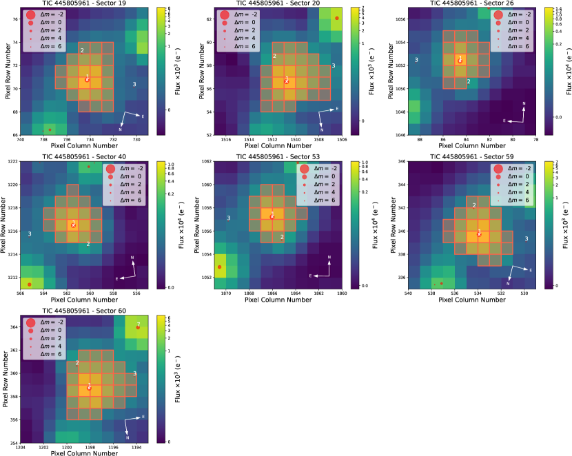
Figure 8: TESS target pixel file image of TOI-1710 (TIC 445805961) observed in Sectors 19, 20, 26, 40, 53, 59, and 60 (made with tpfplotter). The pixels highlighted in red show the aperture used by TESS to obtain the photometry. The electron counts are colour-coded. The positions and sizes of the red circles respectively represent the positions and TESS magnitudes of nearby stars. TOI-1710 is marked with a cross ($\times$) and labelled $\#$1.

The TESS raw data are reduced by the Science Processing Operations Center (SPOC; Jenkins et al., 2016) at the NASA Ames Research Center and are publicly available at the Mikulski Archive for Space Telescopes (MAST). The light curves were extracted using simple aperture photometry (SAP; Morris et al., 2020) and corrected from systematics using the Presearch Data Conditioning (PDC) pipeline (Smith et al., 2012; Stumpe et al., 2012, 2014). For this work we used the PDC-corrected SAP photometry, which is the TESS product also used by König et al. (2022). The TESS pixels considered to compute the SAP and PDC-corrected SAP for Sectors 19, 20, 26, 40, 53, 59, and 60 are shown in Figure 8. A single transit was detected in the Sector 19 PDC-SAP flux time series, and the correct period can be identified in a combined search of the available sectors.

On February 19, 2020, the star was announced under the TESS Object of Interest (TOI) number 1710 as a possible host for a transiting planet in the TOI catalogue (Guerrero et al., 2021). A signal with a period of $24.28$ days and a transit depth ($\Delta F$) of 3070.0 ppm, corresponding to a planet radius of about 5.4 $\mathrm{R}_{\oplus}$, was detected in the Quick Look Pipeline (QLP; Huang et al., 2020a, b ). All SPOC data validation (Twicken et al., 2018; Li et al., 2019) diagnostic test results for this signal are fully consistent with a transiting planet associated with the host star (within 0.7 $\pm$ 2.6$"$) and excluded all other TIC objects.

2.2 Ground-based photometry

We observed a full transit of TOI-1710.01 on the night of February 29, 2020, with the George Mason University Observatories 0.8 m telescope. We used the TESS Transit Finder to schedule our transit observation (Jensen, 2013). We utilized AstroImageJ (Collins et al., 2017) for data reduction, plate-solving, aperture photometry, light curve extraction, and detrending. Due to differences in quality and scattering between space- and ground-based measurements, we analysed the two datasets individually, focusing our photometric analyses on the TESS light curves, and we did not include these observations in the joint fit modelling in Sect. 4.3. However, ground-based observations are key to the independent confirmation and validation of TESS candidates.

2.3 High-resolution spectroscopy with SOPHIE

König et al. (2022) performed a ground-based follow-up campaign with the SOPHIE spectrograph. They obtained a total of 30 RV measurements acquired from September 14, 2020, to May 7, 2021. The details of these observations are explained in Sect. 2.2.2 of König et al. (2022).

2.4 High-resolution spectroscopy with HARPS-N

TOI-1710 was observed with the High Accuracy Radial velocity Planet Searcher for the Northern hemisphere (HARPS-N; Cosentino et al., 2012) mounted on the 3.6m Telescopio Nazionale Galileo (TNG) at the Roque de los Muchachos Observatory, La Palma. The star was monitored first from October 27, 2020, to April 5, 2021, and then from September 12, 2021, to April 4, 2022. We obtained a total of 54 high-resolution ($R\sim 115\,000$) spectra. The observations were carried out as part of observing programs CAT20B_41 and CAT21A_24 (PI: Pallé). The exposure times varied from 680 to 2400 seconds, depending on weather conditions and scheduling constraints, leading to a S/N per pixel of 33–106 at 5500 Å. The spectra were extracted using the offline version of the HARPS-N DRS pipeline (Cosentino et al., 2014), version 3.7. Doppler measurements (absolute RVs) and spectral activity indicators (cross-correlation function full width at half maximum, FWHM; cross-correlation function contrast, CTR; cross-correlation function bisector, BIS; and $R_{\rm HK}$) were measured using an online version of the DRS, the YABI tool, by cross-correlating the extracted spectra with a G2 mask (Baranne et al., 1996). We also used the serval code (Zechmeister et al., 2018) to measure relative RVs by template-matching, chromatic index (CRX), differential line width (dLW), and H$\alpha$, sodium Na D1 and Na D2 indexes. The uncertainties of the RVs measured with serval are in the range 0.8–2.6 $\mathrm{m\,s^{-1}}$, with a mean value of 1.4 $\mathrm{m\,s^{-1}}$. The uncertainties of absolute RVs measured with DRS are in the range 0.8–3.2 $\mathrm{m\,s^{-1}}$, with a mean value of 1.5 $\mathrm{m\,s^{-1}}$. Table 6 gives the time stamps of the spectra in BJD_TDB serval relative RVs along with their $1\sigma$ error bars, and spectral activity indicators measured with YABI and serval.

König et al. (2022) also performed a ground-based follow-up campaign with HARPS-N, and obtained 31 measurement acquired from October 3, 2020, to April 19, 2021. König et al. (2022) measurements from SOPHIE and HARPS-N are contemporaneous with our first observing campaign. Moreover, there are no significant differences between the two HARPS-N datasets: consistent exposure times, similar S/N per pixel, and measured RV uncertainties, and the same instrumental mode. For consistency, we reduced their HARPS-N spectra together with our HARPS-N observations, with the YABI tool and the HARPS-N DRS pipeline. The RV values (from the König et al. 2022 spectra) extracted using the DRS pipeline are exactly the same as those presented in König et al. (2022, Table C.2). We ran the serval pipeline over both datasets, considering them a single dataset of 85 HARPS-N RVs. The RVs extracted by serval are used in the analyses of this work.

2.5 High-resolution imaging with Gemini/‘Alopeke

Figure 1: Gemini/‘Alopeke high-resolution image of TOI-1710 take on February 9, 2021. TOI-1710 is a single star to contrast limits of 5.5 to 7 mag within 1.6 AU out to 97 AU (d = 81 pc). The inset shows a 1.2”$\times$1.2” reconstructed image of TOI-1710 at 832 nm band, centred on the star.

If an exoplanet host star has a spatially close companion, that companion (bound or line of sight) can create a false-positive transit signal if it is, for example, an eclipsing binary. Additionally, ‘third-light’ flux from the close companion star can lead to an underestimated planetary radius if not accounted for in the transit model (Ciardi et al., 2015) and cause non-detections of small planets residing within the same exoplanetary system (Lester et al., 2021). The discovery of close-in bound companion stars, which exist in nearly one-half of FGK-type stars (Matson et al., 2018), provides crucial information towards our understanding of exoplanetary formation, dynamics, and evolution (Howell et al., 2021). Thus, to search for close-in bound companions, unresolved in TESS or other ground-based follow-up observations, we obtained high-resolution imaging speckle observations of TOI-1710.

TOI-1710 was observed on February 9, 2021, using the ‘Alopeke speckle instrument on the Gemini North 8 m telescope. ‘Alopeke provides simultaneous speckle imaging in two bands (562 nm and 832 nm) with output data products including a reconstructed image with robust contrast limits on companion detections (e.g. Howell et al., 2016). Seven sets of 1000$\times$0.06 sec exposures were collected and subjected to Fourier analysis in our standard reduction pipeline (see Howell et al., 2011). Figure 1 shows our final contrast curves and the 832 nm reconstructed speckle image. We find that TOI-1710 is a single star with no companion brighter than 5.5–7 magnitudes below that of the target star from the diffraction limit (20 mas) out to 1.2”. At the distance of TOI-1710 (d = 81 pc) these angular limits correspond to spatial limits of 1.6 to 97 AU.

3 Stellar system analysis

Table 1: Stellar parameters of TOI-1710.

Parameter	Value	Reference
Name and identifiers
TIC	445805961	TESS
TOI	1710	TOI
BD	+76 227	BD
TYC	4525–1009–1	TYC
2MASS	J06170789+7612387	2MASS
Gaia DR2	1116613161053977472	Gaia
Coordinates and spectral type
$\alpha$ (J2000)	06${}^{\mathrm{h}}\,$17m 07${}^{\mathrm{s}}\!$.86	Gaia
$\delta$ (J2000)	$+$76º 12′ 38$"\!$.81	Gaia
Spectral type	G5 V	W03
Parallax and kinematics
$\pi$  [mas]	12.2823 $\pm$ 0.0266	Gaia
$d$  [pc]	81.42 $\pm$ 0.18	Gaia
$\mu_{\alpha}\cos{\delta}$  [mas year-1]	59.837 $\pm$ 0.037	Gaia
$\mu_{\delta}$  [mas year-1]	55.610 $\pm$ 0.044	Gaia
$V_{\rm r}$  [$\mathrm{km\,s^{-1}}$]	$-$39.40 $\pm$ 0.35	Gaia
	$-$38.8134 $\pm$ 0.0007	Sec. 2.4
Magnitudes
B [mag]	10.20 $\pm$ 0.03	TYC
V [mag]	9.54 $\pm$ 0.02	TYC
G [mag]	9.3598 $\pm$ 0.0002	Gaia
T [mag]	8.9134 $\pm$ 0.006	TESS
J [mag]	8.319 $\pm$ 0.019	2MASS
H [mag]	8.003 $\pm$ 0.034	2MASS
K [mag]	7.959 $\pm$ 0.026	2MASS
Stellar parameters
Mass  $M_{\star}$ [$M_{\odot}$]	0.99 $\pm$ 0.07	Sec. 3.3
	0.984${}^{+0.050}_{-0.059}$	K22
Radius  $R_{\star}$ [$R_{\odot}$]	0.95 $\pm$ 0.02	Sec. 3.3
	0.968${}^{+0.016}_{-0.014}$	K22
Luminosity  $L_{\star}$ [$L_{\odot}$]	0.895 $\pm$ 0.003	Gaia
Effective temperature  $T_{\rm eff}$ [K]	5730 $\pm$ 30	Sec. 3.3
	5665 $\pm$ 55	K22
Surface gravity  $\log$(g)	4.54 $\pm$ 0.09	Sec. 3.3
	4.46 $\pm$ 0.10	K22
Metallicity  $\rm[Fe/H]$	0.12 $\pm$ 0.06	Sec. 3.3
	0.10 $\pm$ 0.07	K22
Age  [Gyr]	2.8 $\pm$ 0.6	Sec. 3.2
	4.2${}^{+4.1}_{-2.7}$	K22
log(R${}^{{}^{\prime}}_{HK}$)	$-$4.786 $\pm$ 0.012	Sec. 3.2
	$-$4.78 $\pm$ 0.03	K22

TESS: Stassun et al. (2018, 2019), TOI: Guerrero et al. (2021), BD: Argelander (1903), TYC: Høg et al. (2000); Gaia: Gaia Collaboration et al. (2018); Gaia Collaboration (2020); 2MASS: Cutri et al. (2003); W03: Wright et al. (2003); K22: König et al. (2022).

3.1 Stellar companions

Given the fainter TOI-1710 companion labelled $\#$2 in Figure 8 and the large TESS pixel size of 21”, it is crucial to verify that no visually close-by targets are present. In Section 2.5 we ruled out this scenario within 1.2” around TOI-1710 (see Fig. 1). To go wider, we extended the exploration of close companions until 60” around the star position using the Gaia DR2 (Gaia Collaboration et al., 2018) database. The main astrometric parameters and properties of the five found objects, relative to TOI-1710, are included in Table 2.

Gaia DR2 1116613161052594560 at 7.2” with G_RP = 17.4 mag is the only target within one TESS pixel, but it is much fainter than TOI-1710 (G_RP = 8.9 mag). Stars with differences in Gaia G_RP-band larger than 8 mag are not detected in the TESS images (Figure 8). Only Gaia DR2 1116612783096856960, which has $\Delta$ G_RP = 4.2 mag, is detected. We identified this star as TIC 445805957, which is the southern star labelled $\#$2 in Figure 8. Since star $\#$2 has a parallax and proper motion similar to that of TOI-1710, we can assume that they are probably gravitationally bounded. This is in agreement with Mason et al. (2001) and Tian et al. (2020), who reported this pair of stars as a wide binary system.

Because the Gaia G_RP-band (630–1050 nm) and the TESS band (600–1000 nm) are very much alike, we could estimate the dilution factor for the TESS photometry (D${}_{\textit{TESS}}$) using its definition from Eq. 6 in Espinoza et al. (2019). We calculated a D${}_{\textit{TESS}}$ = 0.988 considering all the nearby stars, corresponding to 1.2% flux contamination. However, the PDC-corrected SAP light curve, which is the data used in the photometry and joint fit analyses (Sections 4.2 and 4.3), already takes into account the possible flux contamination by the nearby companion, which is by far the brightest close star. Excluding the flux from TIC 445805957 from the calculations, D${}_{\textit{TESS}}$ is 0.999 (i.e. consistent with little to no flux contamination).

Table 2: Relative properties to TOI-1710 of the nearby stars. TOI-1710 wide binary companion Gaia DR2 identifier is marked in bold.

Gaia	Separation	$\Delta$ Parallax	$\Delta$ Proper motion	$\Delta$ GRP
DR2	[ ” ]	[ mas ]	[ mas/year ]	[ mag ]
1116613161052594560	7.2 $\pm$ 0.1	12.0 $\pm$ 0.2	72.66 $\pm$ 0.14	8.545 $\pm$ 0.025
1116613225476795776	30.8 $\pm$ 0.1	12.30 $\pm$ 0.25	79.35 $\pm$ 0.14	9.153 $\pm$ 0.020
1116613195412077696	37.1 $\pm$ 0.1	10.9 $\pm$ 0.7	72.2 $\pm$ 0.5	10.292 $\pm$ 0.050
1116613225476796288	42.1 $\pm$ 0.1	12.1 $\pm$ 0.3	80.02 $\pm$ 0.17	9.592 $\pm$ 0.020
1116612783096856960	43.3 $\pm$ 0.1	0.0 $\pm$ 0.06	0.087 $\pm$ 0.003	4.2307 $\pm$ 0.0018

3.2 Stellar rotation

Based on the Noyes et al. (1984) and Mamajek & Hillenbrand (2008) activity-rotation relations and using (B-V) of 0.658 and the $\log\,R^{{}^{\prime}}_{HK}$ measured with YABI, we estimated a rotation period of TOI-1710 for 20.9 $\pm$ 4.2 days and 20.6 $\pm$ 3.2 days, respectively. Using the activity-age relation of Mamajek & Hillenbrand (2008), we also found the age of TOI-1710 to be in the range of 2.2–3.9 Gyr.

We searched for photometric time series from automated ground-based surveys to detect long-term photometric modulations associated with the stellar rotation. The Northern Sky Variability Survey (NSVS; Woźniak et al., 2004) is the only public survey in which the search was successful. The search parameters were the TOI-1710 coordinates from Table 1 and a radius of 1’ around it.

The query returned two objects labelled with different identifiers: ($i$) $\#$594837 (RA = 06:17:07.86, Dec = +76:12:38.23, and magnitude = 9.657 $\pm$ 0.011 mag with a scatter magnitude of 0.024 mag) and ($ii$) $\#$628193 (RA = 06:17:07.88, Dec = +76:12:38.41, and magnitude = 9.671 $\pm$ 0.011 mag with a scatter magnitude of 0.021 mag). Objects $\#$594837 and $\#$628193 are only separated from each other by 0.20” and they are 0.58” and 0.41” apart from TOI-1710, respectively. Their magnitudes are coincident within the scatter magnitudes and they are only 0.1 mag apart from TOI-1710 V-band magnitude. Since we already confirmed in Section 3.1 that there is no other star of similar magnitude within 60” around TOI-1710, we can safely assume that the NSVS observations of $\#$594837 and $\#$628193 correspond to the same object, TOI-1710.

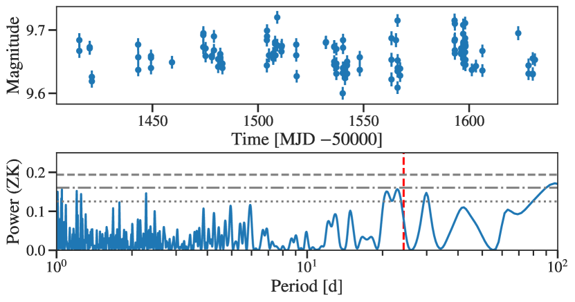
Figure 2: Dataset (top) and generalized Lomb-Scargle periodogram (bottom) of Northern Sky Variability Survey photometric data for TOI-1710. The vertical red dashed line marks the 24.28 d period. The 10%, 1%, and 0.1% FAP levels are indicated by horizontal grey dotted, dash-dotted, and dashed lines, respectively.

We searched for photometric periodicities in the total of 117 NSVS measurements using the generalized Lomb-Scargle (GLS) periodogram (Zechmeister & Kürster, 2009). In addition, we computed the theoretical false alarm probability (FAP), as described in Zechmeister & Kürster (2009). The photometry and its GLS periodogram are shown in Figure 2. A baseline of 216 days should be enough to detect any significant photometric modulation in the expected range for the stellar rotational period. The only relevant signal is a broad double peak in the range 20–24 d with a FAP close to the 1%, and consistent with the $P_{\rm rot}$ reported by König et al. (2022) of $\sim$22 d.

3.3 Stellar parameters

The analysis of the stellar spectrum was carried out by using the BACCHUS code (Masseron et al., 2016) relying on the MARCS model atmospheres (Gustafsson et al., 2008) and using the co-added HARPS-N spectra. In brief, an effective temperature of 5730 $\pm$ 10 K was derived by requiring no trend of the Fe I lines abundances against their respective excitation potential. The surface gravity was determined by requiring the ionization balance of the Fe I and Fe II lines. A microturbulence velocity value of 0.89 $\pm$ 0.05 $\mathrm{km\,s^{-1}}$ was also derived by requiring no trend of Fe line abundances against their equivalent widths. The output metallicity ($+0.12$ $\pm$ 0.06) is represented by the average abundance of the Fe I lines. An alternative analysis of the HARPS-N spectrum was done with the SPC pipeline (Buchhave et al., 2012). The results obtained with this pipeline are $T_{\rm eff}$ = 5720 $\pm$ 28, $\log g$ = 4.49 $\pm$ 0.04, and $\rm[M/H]$ = $+$0.06 $\pm$ 0.04. These results are consistent with the parameters derived with the BACCHUS pipeline. Nevertheless, the internal error in temperature that was derived for example by the BACCHUS code (10 K) or the SPC code (28 K) are unrealistically small as they do not include systematic errors. One of the main known sources of uncertainties are NLTE or 3D effects that are not considered in either of the 1D/LTE analyses of the HARPS-N spectrum. In order to try to better estimate its global error, the effective temperature was also derived with photometry. While the spectroscopic method we employed relies on individual line strengths of the observed stellar spectrum, the photometric method relies on the relative flux of the star and its observed colours. In that sense, one can consider that the spectroscopic and the photometric method provide fairly independent results, and thus better reflect the absolute uncertainty on temperature. Nevertheless, the photometric method also has its own uncertainties. To minimize the error, we chose the V-K colour index. This index has been demonstrated to be the most robust and most reliable temperature indicator because it offers a wider baseline of the spectral energy distribution and because it is less dependent on other parameters, such as metallicity and surface gravity (Bessell et al., 1998; Casagrande et al., 2010). Another known source of uncertainty of the photometric method resides in the absolute calibration that sets the zero-point of the $T_{\rm eff}$ scale; this calibration varies from one study to another. By using the V-K colour-temperature relation of González Hernández & Bonifacio (2009) and that of Casagrande et al. (2010) and assuming no reddening for such a close-by star, we obtained a temperature of 5669 $\pm$ 32 K and 5719 $\pm$ 25 K, respectively. While all photometric and spectroscopic temperatures are in good agreement, we chose to compute the error in temperature by taking half of the difference between the most extreme spectroscopic and photometric temperatures, which are the BACCHUS and the González Hernández & Bonifacio (2009) temperatures, leading to a total error of 30 K.

In a second step, we used the Bayesian tool PARAM (Rodrigues et al., 2014, 2017) to derive the stellar mass, radius, and age utilizing the spectroscopic parameters and the updated Gaia luminosity along with our spectroscopic temperature. However, these Bayesian tools underestimate the error budget as they do not take into account the systematic errors between one set of isochrones to another, due to the various underlying assumptions in the respective stellar evolutionary codes. In order to take into account those systematic errors, we combined the results of the two sets of isochrones provided by PARAM (i.e. MESA and Parsec) and added the difference between the two sets of results to the error budget provided by PARAM. We obtained a stellar radius and mass of $\rm 0.95\pm 0.02\,R_{\odot}$ and $\rm 0.99\pm 0.07\,M_{\odot}$, respectively. We note, however, that although using two sets of isochrones may mitigate underlying systematic errors, our formal error budget for radius and luminosity may still be underestimated, as demonstrated by Tayar et al. (2022). For solar-type stars such as TOI-1710, absolute errors may instead be up to 4%, 2%, 5%, and 20% respectively for radius, luminosity, mass, and age.

The derived age from the isochrones (3.2 $\pm$ 3.1 Gyr) do not provide constraining information as age is very degenerate for stars on the main sequence (see Fig. 3) . Therefore, we rely on the study of Mamajek & Hillenbrand (2008) for the choice of the age (2.8 $\pm$ 0.6 Gyr) derived from the empirical R${}^{{}^{\prime}}_{HK}$-age relation.

All stellar parameters adopted in our joint modelling of the system (presented in Section 4) are summarized in Table 1. In Table 1 are also displayed the values provided by König et al. (2022). The values are in good agreement, although we derive a slightly higher temperature. The method employed to derive the temperature in König et al. (2022) is very similar to ours, and the small discrepancy is likely due to the differences in the model atmosphere, radiative transfer codes, and the selection of Fe lines, as demonstrated in Jofré et al. (2014). While such a difference in temperature consistently leads to a slightly higher mass and smaller radius between the two studies, $M_{\star}$, $R_{\star}$, log(g), metallicity, age, and log(R${}^{{}^{\prime}}_{HK}$) are still in agreement within the error bars.

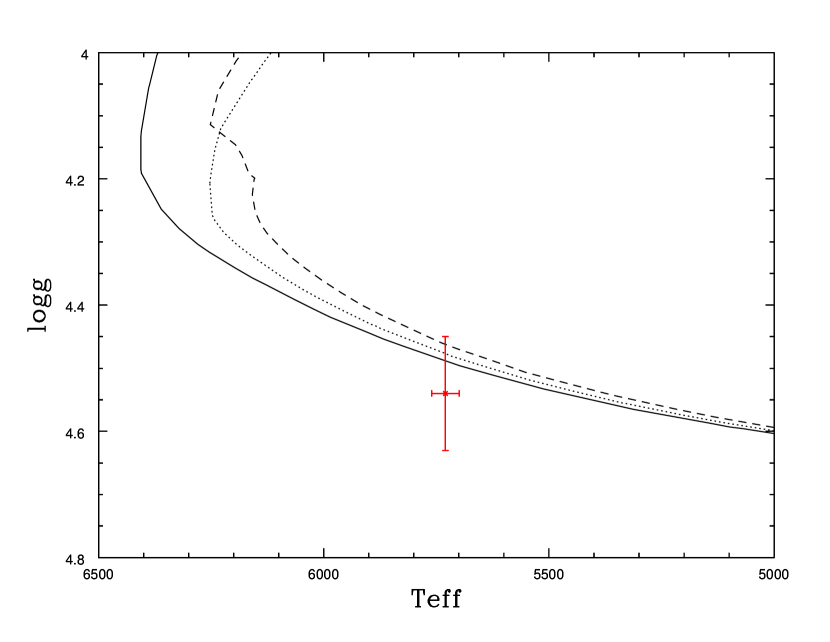
Figure 3: Location of the host star in the spectroscopic H-R diagram. The red point and error bars indicate the spectroscopic parameters of the host star, while the solid, short-dashed, and long-dashed lines show isochrones for 2.5, 3.0, and 4.0 Gyr, respectively.

4 Analysis

4.1 Frequency analysis and RV correlations

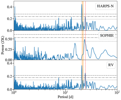
Figure 4: Generalized Lomb-Scargle periodograms of HARPS-N, SOPHIE, and combined RV measurements (from top to bottom). Vertical red dotted line indicates the period of TOI-1710 b at 24.28 d. Shaded orange region indicates the 3$\sigma$ region of the $P_{\rm rot}$ from the joint fit (see Sect. 4.3). The graph shows 10%, 1% and 0.1% FAP levels in grey dotted, dash-dotted, and dashed, respectively.

Our RV dataset involves a total of 115 measurements from HARPS-N (85) and SOPHIE (30) spectrographs with a time baseline of 217 days. We searched for TOI-1710 b and other signals in the HARPS-N, SOPHIE, and combined RV datasets computing their GLS periodograms, which are shown in Figure 4. The signal of the planet is well detected in the RV datasets with FAP $\lesssim$ 1 %. However, the biggest peak in the HARPS-N and the combined dataset periodograms is at $\sim$20 days, which is consistent with the rotation period of the star derived in Sect. 3.2 and by König et al. (2022). Thus, the RVs analysed in this work have two clear signals that have to be modelled: the transiting planet TOI-1710 b at 24.28 d, and the stellar rotation at 20–22 d. Due to the proximity of the two signals, they should be treated with caution when analysing the RVs.

We computed the GLS periodogram of the HARPS-N activity parameters measured with YABI and serval (see Figure 12). In general, all the activity periodograms present peaks in the region where the stellar rotation is expected (20–24 d). These peaks are significant (FAP ¡ 1 %) for CTR, FWHM, dLW, Na D1, and $R_{\rm HK}$. All the activity indicators except CRX and Na D2 also present significant peaks at $\sim P_{\rm rot}/2$. König et al. (2022) also presented the GLS periodograms for FWHM, H$\alpha$, and log(R‘_HK) with significant peaks close to the stellar rotation period. Moreover, the HARPS-N CTR, FWHM, dLW, and H$\alpha$ index have strong correlations with the HARPS-N RVs (see Fig. 13). Similar correlations are obtained when we split the HARPS-N dataset in two (before and after September 2021), indicating that the stellar correlation did not come (only) from the second epoch and that it is present over all the observations. The stellar rotation detected in the RV GLS periodogram and the correlation of the RVs with the FWHM, for example, are not negligible.

4.2 Photometric modelling

In a first step, previous to the RV and photometry simultaneous analysis, we studied the photometric data alone. Although TOI-1710 was observed in Sectors 19, 20, 26, 40, 53, 59, and 60, the TOI-1710 b expected transit in Sector 60 fell in the mid-sector observing gap. Thus, we did not consider Sector 60 in our analysis because it has no 1710 b transits, and to save computational time. We analysed the TESS data from Sectors 19, 20, 26, 40, 53, and 59 with the Python library juliet (Espinoza et al., 2019). Juliet performs the fitting procedure using other public packages for modelling of transit light curves (batman, Kreidberg, 2015) and GPs (celerite, Foreman-Mackey et al., 2017). Instead of using the Markov chain Monte Carlo (MCMC) technique, juliet uses a nested sampling algorithm (dynesty, Speagle, 2020; MultiNest, Feroz et al., 2009; Buchner et al., 2014) to explore the whole the parameter space. We considered the uninformative sample ($r_{1}$,$r_{2}$) parametrization introduced in Espinoza (2018) to explore the impact parameter of the orbit ($b$) and the planet-to-star radius ratio ($p$ $=$ ${R}_{\mathrm{p}}/{R}_{\star}$) values. In the fitting procedure we adopted a quadratic limb-darkening law with the ($q_{1}$,$q_{2}$) parametrization introduced by Kipping (2013). According to the flux contamination exploration in Sect. 3.1, we can safely fix the dilution factor to 1. We added a celerite GP exponential kernel to the transiting planet model to account for the extra correlated noise in the photometric data.

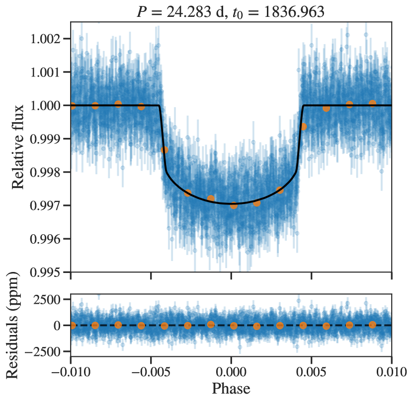
Figure 10: TOI-1710 TESS photometry (blue dots with error bars) phase-folded to the period $P$ and central time of transit $t_{0}$ (shown above each panel, $t_{0}$ units are BJD $-$ 2 457 000) derived from the juliet fit. The black line is the best transit model for TOI-1710 b. The orange points show the binned photometry for ease of visualization. The GP model was removed from the data.

The fitted parameters with their prior and posterior values, and the derived parameters are shown in Table 5. The TESS data along with the transiting and GP models are shown in Fig. 9. The TOI-1710 b phase-folded photometry from the juliet anaysis is shown in Fig. 10. The results from the photometric data analysis are consistent with the planetary characteristics from König et al. (2022).

Furthermore, we analysed the ground-based TOI-1710 b transit modelling the airmass-detrended light curve with ExoFASTv2 (Eastman et al., 2019) to validate the detection. The independent analysis confirmed the results derived from the TESS light curves, and we recovered a $8\sigma$ significance and on-time and on-target transit with consistent depth, duration, and timing with the TESS ephemerides. Ground-based photometry along with its transit fit is shown in Figure 11.

4.3 Joint fit modelling

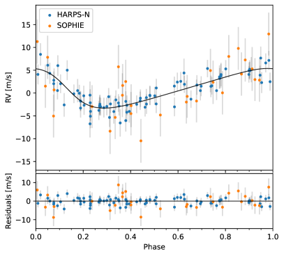
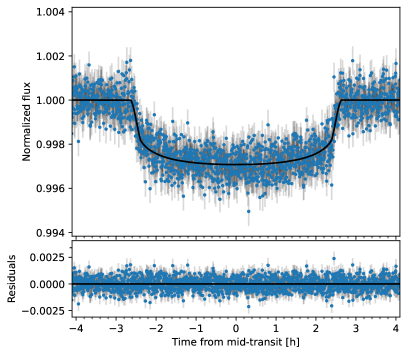
Figure 5: Phase-folded RV (top) and TESS (bottom) data for TOI-1710 b. Upper panel: HARPS-N (blue) and SOPHIE (orange) RV data with the overplotted fit from the 1pGP model. Lower panel: Combination of TESS transits from Sectors 19, 20, 26, 26, 40, 53, and 59. The black line is the inferred 1pGP model.

Table 3: Statistical criteria for the three tested models. Listed are the model names, BIC and AIC values, and number of free parameters. The best criteria model is marked in bold.

Model	BIC	AIC	$N_{\mathrm{free}}$
1p	$-$61120.8	$-$61370.8	38
1pGP	$-$61116.9	$-$61399.8	43
1pGP+FWHM	$-$61340.0	$-$61643.4	46

Table 4: TOI-1710 parameters from the transit and RV joint fit, obtained with the model 1pGP.

Parameter	Prior(a)	Value(b)
Model Parameters
Orbital period $P_{\mathrm{orb}}$ [days]	$\mathcal{U}[24.18,24.38]$	$24.283382\pm 0.000019$
Transit epoch $T_{0}$ [BJD - 2 450 000]	$\mathcal{U}[9025.00,9037.00]$	$9031.23007_{-0.00037}^{+0.00041}$
$\sqrt{e}\sin\omega_{\star}$	$\mathcal{U}(-1,1)$	$0.42\pm 0.13$
$\sqrt{e}\cos\omega_{\star}$	$\mathcal{U}(-1,1)$	$-0.01\pm 0.10$
Scaled planetary radius $R_{\mathrm{p}}/R_{\star}$	$\mathcal{U}[0,0.5]$	$0.048\pm 0.0004$
Impact parameter, $b$	$\mathcal{U}[0,1]$	$0.081_{-0.058}^{+0.093}$
Radial velocity semi-amplitude variation $K$ [m s-1]	$\mathcal{U}[0,50]$	$4.20\pm 1.0$
Derived parameters
Planet radius [$R_{\rm J}$]	$\cdots$	$0.460\pm 0.010$
Planet radius [$R_{\oplus}$]	$\cdots$	$5.15\pm 0.12$
Planet mass [$M_{\rm J}$]	$\cdots$	$0.058_{-0.014}^{+0.015}$
Planet mass [$M_{\oplus}$]	$\cdots$	$18.4_{-4.5}^{+4.8}$
Eccentricity $ecc$	$\cdots$	$0.185_{-0.091}^{+0.12}$
Scaled semi-major axis $a/R_{\star}$	$\cdots$	$30.6_{-3.9}^{+3.1}$
Semi-major axis $a$ [AU]	$\cdots$	$0.164\pm 0.004$
$\omega_{\rm P}$ (deg)	$\cdots$	91 $\pm$ 14
Orbital inclination $i$ (deg)	$\cdots$	$89.8\pm 0.3$
Transit duration $T_{14}$ [days]	$\cdots$	$0.263_{-0.024}^{+0.037}$
Transit duration $T_{23}$ [days]	$\cdots$	$0.238_{-0.021}^{+0.033}$
Equilibrium temperature(c) $T_{\rm eq}$ [K]	$\cdots$	$730_{-30}^{+36}$
Planet instellation ${S}$ [$\mathrm{S}_{\oplus}$]	$\cdots$	$33\pm 2$
Other system parameters
Jitter term $\sigma_{\rm HARPS-N}$ [m s-1]	$\mathcal{U}[0,60]$	$1.40_{-0.33}^{+0.35}$
Jitter term $\sigma_{\rm SOPHIE}$ [m s-1]	$\mathcal{U}[0,60]$	$4.4_{-1.2}^{+1.3}$
Stellar density $\rho_{\star}$ [$\rho_{\odot}$]	–	$0.65\pm 0.22$
Limb darkening $q_{1}$	$\mathcal{N}[0.226,0.090]$	$0.293\pm 0.062$
Limb darkening $q_{2}$	$\mathcal{N}[0.52,0.21]$	$0.34\pm 0.11$
Stellar activity GP model Parameters
$h_{\rm HARPS-N}$ [m s-1]	$\mathcal{U}[0,100]$	$6.5_{-1.1}^{+1.4}$
$h_{\rm SOPHIE}$ [m s-1]	$\mathcal{U}[0,100]$	$4.4_{-2.3}^{+2.4}$
$\lambda$ [days]	$\mathcal{U}[5,2000]$	$62_{-12}^{+15}$
$\omega$	$\mathcal{U}[0.01,1.50]$	$0.375_{-0.088}^{+0.110}$
$\theta$ (Prot) [days]	$\mathcal{U}[2,40]$	$21.51_{-0.24}^{+0.23}$

Note – ^(a) $\mathcal{U}[a,b]$ refers to uniform priors between $a$ and $b$; $\mathcal{N}[a,b]$ refers to Gaussian priors with median $a$ and standard deviation $b$.
^(b) Parameter estimates and corresponding uncertainties are defined as the median and the 16th and 84th percentiles of the posterior distributions.
^(c) Assuming zero Bond albedo.

We performed a joint fit using only TESS photometry and RV data using PyORBIT (Malavolta et al. 2016, 2018) in order to obtain the planetary system parameters. For the fit of transit light curves, this code makes use of the public package batman (Kreidberg, 2015) and allows Gaussian processes (GPs) to be included through the george package (Ambikasaran et al., 2014) in order to model the presence of correlated noise or systematic effects in the data. The parameter space is sampled by using the MCMC technique with the ensemble sampler emcee (Foreman-Mackey et al., 2013). The initial conditions are obtained with the global optimization code PyDE. We use the GP quasi-periodic kernel, as defined by Grunblatt et al. (2015), imposing a uniform prior on the rotational period $P_{\rm rot}$. To run the GPs, we used 10 000 steps, 184 walkers, a burn-in cut of 1 000, and a thinning factor of 100. The confidence intervals of the posterior distributions are computed considering the 34.135th percentile from the median.

Regarding the photometric TESS light curves, we modelled the time of first transit $T_{c}$, the orbital period $P$, the limb darkening (LD) with Kipping (2013) parametrization, the impact parameter $b$, and the scaled planetary radius $R_{P}/R_{\star}$. The eccentricity $ecc$ and argument of periastron $\omega$ were modelled with the parametrization from Eastman et al. 2013 ($\sqrt{e}\cos\omega$,$\sqrt{e}\sin\omega$). We used Gaussian priors both for the stellar mass and radius (as obtained in Sect. 3.3) and for the LD coefficients (calculated with PyLDTk; Parviainen & Aigrain 2015; Husser et al. 2013). The stellar density and the impact parameter $b$ were left free. In order to save computational time, we only used the TESS data around TOI-1710 b transits.

The RV data are modelled taking into account the offset between different instruments, and a jitter term for systematics and stellar noise. The joint fit was performed for three models: i) one planet without GP (1p); ii) one planet with GP (1pGP); iii) one planet with GP and FWHM included in the GP (1pGP+FWHM). This last model, where the GP is fed with the FWHM values, was tested because of the strong correlation between the FWHM and the HARPS-N RVs (Fig. 13). We computed the Bayesian criteria in order to evaluate their significance. In particular, we computed the Bayesian information criterion (BIC) and the Akaike information criterion (AIC); the 1pGP+FWHM model is strongly preferred over the other two models (see Table 3), indicating that the activity plays an important role in the data. This is also proved by the RV residuals, which are quite flat with no extra significant signals (FAP$\gg$10%), when adopting the GP in the model (see Fig 14). The priors, posteriors, and derived planetary parameters from the 1pGP+FWHM model are presented in Table 4. The phase-folded TESS photometry and RVs are shown in Fig. 5.

König et al. (2022) also detected the $P_{\rm rot}$ in their activity indicators GLS periodograms, but the stellar rotation was not strong in their RV periodogram. No correlation plots (e.g. Fig. 13) are shown. They tested three RV models with different GP kernels (one of which is the quasi-periodic kernel used in our analysis), and found values and uncertainties in good agreement with those obtained when no GP was included. However, they modelled the RV data with the juliet code (Espinoza et al., 2019), whose GPs can only be fed by the time stamps, as in our 1pGP model. The 1p and 1pGP models have no clear Bayesian criterion preference, but 1pGP+FWHM does (Table 3). Although the $P_{\rm rot}$ and the planet period peaks are clear in the GLS periodogram (Fig. 4), they are close. Thus, it is expected that, when modelling the two models simultaneously, the semi-amplitude is smaller than the one obtained when only the planet Keplerian is considered (as in König et al., 2022). The semi-amplitudes obtained in this work and by König et al. (2022) differ by 1.6$\sigma$. Moreover, although our analyses included 54 more RVs, the fitted semi-amplitude has the same uncertainties ($\pm$1.0 m s^-1) as that of König et al. (2022). This may be explained by the addition of the GP in the model, and in fact the semi-amplitude uncertainty obtained with our 1p model is 0.8 m s^-1.

By adding two more TESS transits in the joint fit analysis, we improved the photometric parameters. We reduced the $P$, $T_{0}$, and $R_{\rm p}/R_{\star}$ uncertainties from 4.3$\cdot$10^-5, 4.2$\cdot$10^-4, and 6$\cdot$10^-4 in König et al. (2022) to 1.9$\cdot$10^-5, 3.7$\cdot$10^-4, and 4$\cdot$10^-4, respectively. However, the uncertainty for $R_{\rm p}$ did not improve (this work: 0.12 $\mathrm{R}_{\oplus}$; König et al. (2022): 0.11 $\mathrm{R}_{\oplus}$), meaning that the main source of uncertainty comes from $R_{\star}$.

5 Discussion and conclusions

From our analyses, we derive for the transiting sub-Saturn planet TOI-1710 b a radius of $R_{\rm p}$ $=$ 5.15 $\pm$ 0.12 $\mathrm{R}_{\oplus}$, a mass of $M_{\rm p}$ $=$ 18.4 ${}^{+4.8}_{-4.5}$ $\mathrm{M}_{\oplus}$, and a mean bulk density of $\rho_{\rm p}$ $=$ 0.73 $\pm$ 0.18 $\mathrm{g\,cm^{-3}}$, adopting the stellar parameter values from Section 3.3. Our planetary parameters are consistent with those previously derived by König et al. (2022), and we confirmed the eccentric orbit of TOI-1710 b (ecc = 0.185${}_{-0.091}^{+0.12}$). The mass uncertainties are very similar between the two works, but our mean mass measurement value presents a precision at the 4$\sigma$ level, and it is $\sim$1.5$\sigma$ away from that of König et al. (2022, $M_{\rm p}$ $=$ 28.3 $\pm$ 4.7 $\mathrm{M}_{\oplus}$). Although this difference is not significant, we needed to add a GP component accounting for the stellar rotation to successfully fit the RV dataset from this work (see Table 3 and Fig. 14).

After subtracting the 1pGP+FWHM model, the GLS periodograms of the HARPS-N, SOPHIE, and combined RVs are well below the 10 % FAP (see Fig. 14). König et al. (2022) reported an extra peak at 30 d with FAP $\simeq$ 2.2 % after modelling the TOI-1710 b signal. However, here with more RV measurements and after accounting for the stellar rotation, we do not find evidence of any extra signal in the TOI-1710 planetary system.

5.1 Potential atmospheric characterization of TOI-1710 b

TOI-1710 b is a gaseous planet with a scale height ($H$) of $\sim$390 km. As it is expected to posses a significant envelope, we evaluated its suitability for atmospheric characterization via the transmission spectroscopy metric (TSM) proposed by Kempton et al. (2018). TSM takes into account the planet radius, mass, equilibrium temperature, stellar radius, and J magnitude. The formula also includes a scale factor to account for 10 hours of observing time with the James Webb Space Telescope (JWST; Gardner et al., 2006) Near Infrared Imager and Slitless Spectrograph (NIRISS) instrument. According to Table 1 from Kempton et al. (2018), the scale factor for sub-Saturn planets is 1.15. The computed TSM for TOI-1710 b is $\sim$150, which is greater than the threshold TSM of 90 for planets ranging 1.5–10 $\mathrm{R}_{\oplus}$ to be selected as high-quality targets for its atmospheric characterization.

There are only a few sub-Saturn planets around bright stars (J $\leq$ 9) with higher TSM: GJ 436b (J = 6.9 mag, TSM = 481; Butler et al., 2004), HAT-P-11b (J = 7.6 mag, TSM = 202; Bakos et al., 2010), GJ 3470b (J = 8.8 mag, TSM = 270; Bonfils et al., 2012), HD 89345b (J = 8.1 mag, TSM = 114; Van Eylen et al., 2018), WASP-166b (J = 8.4 mag, TSM = 233; Hellier et al., 2019), HD 219666b (J = 8.6 mag, TSM = 142; Esposito et al., 2019), LTT 9779b (J = 8.4 mag, TSM = 185; Jenkins et al., 2020), and TOI-421c (J = 8.5 mag, TSM = 161; Carleo et al., 2020). Among the many species that are expected in TOI-1710 b’s atmosphere, one of the most interesting and accessible would be the He i triplet, which has proved to be a powerful tool for studying extended planetary atmospheres, tracking mass-loss and winds in the upper atmospheres, and even detecting cometary-like atmospheric tails (Nortmann et al., 2018). He i has already been detected in similar sub-Saturns, such as GJ 3470 b (Palle et al., 2020; Ninan et al., 2020), HAT-P-11 b (Allart et al., 2018), and HAT-P-26 b (Vissapragada et al., 2022). We used the rotational period of the star to calculate the expected X-ray and extreme UV emission, using the relations in Wright et al. (2011) and Sanz-Forcada et al. (2011). We estimate an X-ray luminosity of $\log L_{\rm X}$ $=$ 28.07 and a calculated $F_{\rm XUV}$ $\sim$1 W m^-2 irradiance in the 5–504 $\AA$ spectral range at the planet b orbit, similar to the flux received by HD 209458 b, where the He i triplet was positively detected by Alonso-Floriano et al. (2019). This is further supported by the high estimated transmission spectroscopy S/N calculated by König et al. (2022), placing TOI-1710 b as the fourth-best candidate within the sub-Saturn population. It is thus clear that TOI-1710 b is a very appealing target for the atmospheric studies, and strong atmospheric features (e.g. the Na i doublet and K i line at 7701 $\AA$ in the visible or the He i triplet and molecules in the near-infrared) are expected in TOI-1710 b, if they are not veiled by clouds or hazes.

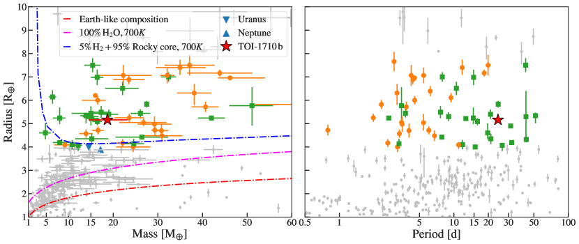
Figure 6: Mass-radius (left) and period-radius (right) diagrams for all known planets with $M_{\rm p}$ $\in$ [1,60] M_⊕ and $R_{\rm p}$ $\in$ [1,10] R_⊕ determined with a precision better than 30% (grey points). The coloured dashed lines are the theoretical mass-radius models from Zeng et al. (2019). Sub-Saturns located in multi-planet systems are marked with green squares, and sub-Saturns located in single-planet systems are orange circles. TOI-1710 b is marked with a red star.

Figure 7: Mass-density (top), mass-eccentricity (middle), and mass-metalicity (bottom) diagrams for the sub-Saturn planets from Fig. 6. Sub-Saturns located in multi-planet systems are marked with green squares and sub-Saturns located in single-planet systems are orange circles. TOI-1710 b is marked with a red star.

5.2 TOI-1710 b within the sample of sub-Saturns

Figure 6 compares TOI-1710 b with known exoplanets, with masses and radii measured with a precision better than 30%, from the NASA Exoplanet Archive along with theoretical composition models of Zeng et al. (2019). The displayed models regard planets with Earth-like composition cores (32.5% Fe + 67.5% MgSiO₂), 100% H₂O composition, and 95% Earth-like rocky core surrounded by 5% H₂ gaseous envelopes. The models are truncated at a reference pressure of 1 mbar and consider an isothermal atmosphere, for which we chose an equilibrium temperature closest to that of TOI-1710 b. Its position in the mass-radius diagram (Fig. 6, left panel), well above the lighter planetary model available (Earth-like composition core with 5% H₂ gaseous envelope), and its bulk mean density ($\rho_{\rm p}$ $=$ 0.75 $\pm$ 0.18 $\mathrm{g\,cm^{-3}}$) suggest that TOI-1710 b may hold a large H–He envelope that could be suitable for spectroscopical exploration, due to the brightness of its host star.

In Figure 6 (and in Figure 7 as well), we marked all other known sub-Saturns detected in multi-planet systems as green squares, while sub-Saturns in single-planet systems (e.g. TOI-1710 b) are shown as orange circles. Figure 6, left panel, shows that lone sub-Saturns tend to be more massive, which is a trend already reported in previous studies (e.g. Petigura et al., 2017, Van Eylen et al., 2018, and Nowak et al., 2020). However, in the intermediate region at 20–30 $\mathrm{M}_{\oplus}$, where TOI-1710 b is located, the two populations are mixed, and there is not a clear boundary line between them. Its closer lone sub-Saturn companion in the mass-radius diagram is TOI-674 b (Murgas et al., 2021), which has an orbital period of less than 2 days ($P$ = 1.97 d).

The right panel in Fig. 6 displays the period-radius diagram, where the TOI-1710 b position seems to be an outlier of the single-planet sub-Saturn population. From this figure we can clearly see that sub-Saturns in multi-planet systems tend to orbit host stars with longer orbital periods than those in single-planet systems. This is unlikely to be an observational or instrumental bias because the lighter planets are the ones farther from their stars. However, because single sub-Saturns have short periods, their possible companions may be in outer orbits. Thus, the hypothetical companions are less likely to transit and should be massive enough to be detectable via radial velocity or astrometry methods. TOI-1710 b has a period of 24 d, and is well within the parameter space of the multi-planet systems; it is the sub-Saturn planet in a single-planet system with the longest period in the diagram. However, there are other sub-Saturn planets with longer periods than TOI-1710 b whose properties have not been determined with precision, for example Kepler-413A b (Kostov et al., 2014) with $P$ = 66 d, and $M_{\rm p}$ $=$ 67 $\pm$ 21 $\mathrm{M}_{\oplus}$. From both panels of Fig. 6, we conclude that single sub-Saturns are more massive and have shorter periods than accompanied sub-Saturns, which are lighter and have longer periods.

Petigura et al. (2017) and Nowak et al. (2020) also explored the possible relations between metallicity, density, and eccentricity of sub-Saturns with planetary mass. In Figure 7 we reproduced these diagrams; TOI-1710 b is indicated with a red star. Other sub-Saturns are marked following the criteria in Fig. 6. Those works found a marginal correlation (Spearman correlation coefficient $r$ = 0.57) between the stellar metallicity and the mass of the sub-Saturns, where massive planets orbit metal-rich stars. A slighly enriched metallicity of $\rm[Fe/H]$ = 0.12 $\pm$ 0.06 dex places TOI-1710 at the centre of the metallicity distribution (see Fig. 7, bottom panel). According to the mass-metallicity correlation, the planet mass should also be in the centre of the planetary masses, which TOI-1710 b is. TOI-1710 b is displayed in central positions in all the panels of Fig. 7, and in the mass-radius diagram (Fig. 6, left panel). Thus, although we have not found evidence of extra planetary signals, further follow-up of the TOI-1710 system will allow us to keep refining the characteristics of the transiting planet, and confirm if TOI-1710 b is alone orbiting its host star or if it is the inner planet of a multi-planet system.

Appendix A Additional light curve figures and tables

Table 5: Prior and posterior distributions from the juliet photometric fit. Prior labels $\mathcal{U}$, $\mathcal{N}$, $\mathcal{F}$, and $\mathcal{J}$ represent uniform, normal, fixed, and Jeffrey’s distribution, respectively.

Parameter	Prior	Posterior
$P$ [d]	$\mathcal{N}(24.28,0.01)$	24.283385 (18)
$t_{0}$ (a)	$\mathcal{N}(1836.96,0.01)$	1836.96299 (48)
ecc (deg)	$\mathcal{F}(0)$	–
$\omega$ (deg)	$\mathcal{F}(90)$	–
$r_{1}$	$\mathcal{U}(0,1)$	0.409${}^{+0.059}_{-0.052}$
$r_{2}$	$\mathcal{U}(0,1)$	0.04990$\pm$0.00037
$\rho_{\star}$ [kg m-3]	$\mathcal{N}(1620,100)$	1617${}^{+36}_{-64}$
$\mu_{\textit{TESS}}$ (ppm)	$\mathcal{N}(0.0,0.1)$	135$\pm$6
$\sigma_{\textit{TESS}}$ (ppm)	$\mathcal{J}(10^{-6},10^{6})$	225$\pm$20
$q_{1,\textit{TESS}}$	$\mathcal{U}(0,1)$	0.23${}^{+0.10}_{-0.07}$
$q_{2,\textit{TESS}}$	$\mathcal{U}(0,1)$	0.52${}^{+0.21}_{-0.17}$
GPσ (ppm)	$\mathcal{J}(10^{-6},10^{6})$	224$\pm$16
GPρ [d]	$\mathcal{J}(10^{-3},10^{3})$	0.93${}^{+0.08}_{-0.07}$

Figure 9: TOI-1710 2 min cadence light curve from TESS Sectors 19, 20, 26, 40, 53, and 59 (blue points with error bars) along with the transit plus GP model (black line) from juliet. Upward-pointing red triangles mark the TOI-1710 b transits.

Figure 11: Light curve from the George Mason University Observatory’s 0.8 m telescope along with the best-fit transit model (red line). The blue points show the original photometric data with a cadence of 20 s; the black points show 30 min binned photometry.

Appendix B Additional radial velocity figures and tables

Table 6: Radial velocities and spectral activity indicators measured from TNG/HARPS-N spectra with serval and DRS. Time stamps from König et al. (2022) spectra are marked in bold. Time series of spectra continue into Table 8.

BJDTBD	RV serval		BIS		CCF_FWHM	CCF_CTR	$\mathrm{\log{R^{`}_{HK}}}$		CRX		dlW
$-$2457000	[$\mathrm{m\,s^{-1}}$]		[$\mathrm{m\,s^{-1}}$]		[$\mathrm{km\,s^{-1}}$]	(%)	—		($\mathrm{m\,s^{-1}\,Np^{-1}}$)		[$\mathrm{m^{2}\,s^{-2}}$]
Val.	Val.	$\sigma$	Val.	$\sigma$	Val.	Val.	Val.	$\sigma$	Val.	$\sigma$	Val.	$\sigma$
2125.664739	10.7	1.84	-12.99	2.559	7.277	48.411	-4.7656	0.0105	4.747	14.819	15.794	3.639
2126.618253	5.06	1.67	-11.391	2.08	7.266	48.511	-4.7681	0.0084	2.654	13.866	7.393	2.634
2127.719329	2.24	1.28	-10.508	1.711	7.267	48.597	-4.7574	0.0122	6.085	10.514	-8.641	2.77
2130.73596	-5.98	2.54	-22.531	4.878	7.26	48.304	-4.8279	0.0149	5.319	20.869	18.585	6.192
2133.711696	-7.68	1.35	-15.256	2.305	7.254	48.632	-4.7963	0.0088	8.868	10.824	-11.958	3.119
2134.756264	-8.96	1.86	-18.148	2.451	7.257	48.622	-4.7663	0.0117	3.603	15.075	-10.429	3.526
2149.682376	5.25	1.5	-11.46	2.096	7.24	48.723	-4.785	0.0071	-7.997	12.821	-4.596	2.747
2150.688883	9.76	1.2	-11.969	1.788	7.244	48.698	-4.7903	0.0061	-16.119	9.969	-0.516	1.78
2151.723635	10.56	1.58	-11.029	2.38	7.246	48.671	-4.7727	0.0097	0.421	12.7	1.356	3.282
2156.742015	-6.31	1.12	-19.71	1.724	7.266	48.596	-4.7887	0.0073	-7.344	9.163	-5.44	2.048
2158.686506	-5.64	1.54	-12.062	2.384	7.221	48.765	-4.7668	0.0326	-7.901	12.921	-12.779	3.158
2160.659656	-7.27	1.24	-17.6	1.771	7.226	48.806	-4.7938	0.0056	9.02	10.47	-13.702	2.157
2172.605447	9.48	1.65	-11.241	2.006	7.267	48.546	-4.794	0.0054	1.762	13.263	0.551	3.3
2188.596847	3.8	1.3	-14.871	1.96	7.272	48.48	-4.7884	0.0151	10.722	10.837	11.812	2.93
2189.64318	-2.69	1.02	-12.606	1.601	7.273	48.569	-4.7596	0.0173	5.66	8.758	0.28	1.761
2190.610672	-1.96	1.41	-15.521	1.949	7.262	48.616	-4.7659	0.0222	3.008	12.432	-5.422	2.553
2191.782237	1.06	1.07	-17.256	1.394	7.264	48.64	-4.771	0.0185	6.011	8.591	-11.408	1.747
2204.493933	-7.09	1.35	-20.915	2.192	7.229	48.741	-4.7981	0.0049	5.84	11.869	-2.912	2.467
2204.673882	-5.85	1.12	-20.256	1.545	7.223	48.788	-4.7929	0.0047	9.047	9.829	-11.423	1.735
2205.499679	-1.43	1.02	-14.768	1.408	7.224	48.78	-4.7944	0.0066	13.736	8.672	-8.102	2.041
2205.685433	-2.5	1.17	-10.185	1.919	7.226	48.75	-4.7814	0.0096	6.871	9.888	-8.062	2.571
2206.4971	-0.27	1.08	-19.432	1.585	7.223	48.743	-4.8021	0.0079	-9.944	9.4	-4.913	2.244
2206.679276	-4.27	2.53	-8.329	4.476	7.236	48.531	-4.8129	0.0078	-29.964	20.502	3.099	4.807
2212.534392	1.0	1.29	-16.177	2.127	7.271	48.518	-4.824	0.0309	-11.427	10.351	3.176	3.029
2215.622998	15.87	1.01	-20.647	1.54	7.273	48.514	-4.7824	0.0079	-3.803	8.19	6.178	2.435
2248.433766	-1.07	1.01	-27.121	1.326	7.217	48.844	-4.82	0.0142	-14.392	8.621	-18.587	1.964
2248.444309	-0.28	1.06	-23.395	1.285	7.219	48.846	-4.8332	0.0133	4.076	9.451	-19.282	1.514
2265.415755	2.88	1.93	-1.549	2.569	7.231	48.685	-4.826	0.0123	21.158	15.537	-1.462	3.367
2265.42869	2.53	1.63	-21.879	2.93	7.229	48.657	-4.8417	0.033	6.113	13.459	-2.513	3.663
2265.560543	2.91	2.07	-6.222	3.436	7.234	48.634	-4.8317	0.0337	-1.784	16.663	-1.651	4.335
2265.57402	3.21	2.01	-7.527	3.0	7.236	48.693	-4.8179	0.0259	-5.787	15.995	-3.218	4.034
2268.426272	-0.98	0.77	-16.31	1.206	7.227	48.803	-4.8096	0.0119	-10.589	6.668	-12.481	1.832
2268.438999	-0.13	0.83	-14.652	1.18	7.231	48.795	-4.8162	0.0118	-11.144	7.11	-13.971	1.68
2268.505815	0.17	1.14	-12.733	1.455	7.227	48.799	-4.8228	0.0172	2.831	9.839	-14.944	1.93
2268.519837	-0.18	1.06	-14.503	1.857	7.232	48.759	-4.8353	0.0102	0.231	8.992	-9.382	2.118
2275.338169	4.42	0.93	-9.129	1.361	7.282	48.475	-4.8152	0.0121	-16.989	7.845	42.678	2.134
2276.48642	-1.04	1.25	-11.031	1.735	7.269	48.524	-4.7992	0.0107	-23.013	10.447	5.285	2.225
2277.409061	-0.89	1.15	-11.649	1.486	7.265	48.585	-4.8085	0.0118	-26.776	9.186	-2.286	2.006
2278.43132	-3.63	1.33	-14.517	1.629	7.268	48.589	-4.7943	0.0117	-19.579	11.132	-3.436	1.95
2287.3862	0.35	1.44	-18.127	2.659	7.248	48.629	-4.8129	0.0103	-6.68	11.78	-5.117	3.686
2289.40115	-3.2	1.31	-16.69	1.773	7.255	48.632	-4.8181	0.0101	-15.986	10.631	-11.952	2.457
2290.341493	1.41	1.08	-20.809	1.347	7.259	48.672	-4.8113	0.0132	-13.846	8.778	19.952	1.925
2294.435475	11.65	1.34	-19.321	1.759	7.282	48.512	-4.7985	0.0179	-21.659	10.892	3.553	2.2
2297.388529	4.62	1.11	-12.736	1.367	7.277	48.519	-4.7866	0.0161	-21.198	8.954	6.262	2.071
2298.383859	7.51	1.46	-13.666	1.986	7.272	48.512	-4.847	0.0223	-29.481	11.714	5.659	2.732
2299.452091	1.09	1.98	-16.992	3.415	7.275	48.391	-4.8706	0.0307	-11.599	16.296	17.651	4.4
2303.371341	-0.39	1.37	-16.247	2.125	7.261	48.583	-4.8367	0.0441	-6.505	10.725	-7.953	3.33
2304.382026	-7.29	1.8	-25.52	2.417	7.266	48.606	-4.815	0.0165	-16.113	14.563	-6.493	3.38
2307.349721	-2.59	1.15	-18.116	1.685	7.256	48.595	-4.8167	0.0182	-8.408	9.098	24.798	2.865
2309.358376	-0.15	1.3	-16.503	1.663	7.219	48.808	-4.8179	0.0091	2.781	10.239	-12.948	2.071
2309.371202	-4.7	1.29	-14.803	1.615	7.221	48.788	-4.8248	0.0104	-3.381	10.303	-16.168	2.449
2310.348335	2.24	2.7	-17.647	4.171	7.218	48.549	-4.8028	0.01	-21.734	20.574	38.414	5.807
2310.388924	-0.26	1.01	-18.428	1.663	7.226	48.777	-4.8568	0.0167	-18.036	7.356	-11.074	2.285
2322.354105	-4.91	2.04	-6.607	2.953	7.252	48.389	-4.8559	0.0308	10.087	17.174	44.35	3.227
2323.352913	-1.43	1.26	-20.516	1.744	7.258	48.563	-4.7567	0.0136	2.532	10.796	27.362	2.544
2324.363167	-1.08	1.52	-14.854	2.11	7.247	48.657	-4.7616	0.0102	7.458	12.643	-20.307	3.142
2469.724254	-9.49	1.48	-27.555	2.283	7.219	48.807	-4.7641	0.0077	21.531	12.308	-17.313	2.829
2469.735454	-11.03	1.32	-16.553	2.147	7.22	48.824	-4.8477	0.0423	-3.082	11.466	-19.027	3.0
2469.745825	-9.52	1.4	-17.314	2.067	7.221	48.815	-4.8086	0.0134	26.204	11.819	-14.525	2.95
2470.700788	-5.58	2.52	-24.563	3.877	7.22	48.715	-4.808	0.0151	15.515	20.619	-17.841	4.693
2470.722284	-7.18	2.48	-12.336	4.005	7.224	48.735	-4.7924	0.0085	-22.477	20.357	-18.624	5.05
2470.741717	-10.08	2.04	-14.927	3.423	7.213	48.738	-4.7746	0.0102	-17.234	16.714	-9.654	3.832
2471.706179	-4.7	1.49	-24.021	2.049	7.215	48.854	-4.7648	0.0101	-1.31	12.23	-21.572	2.816
2471.71689	-4.41	1.34	-19.861	2.018	7.218	48.829	-4.7567	0.0072	5.007	11.085	-17.867	2.701
2548.691205	-2.68	1.2	-20.396	2.187	7.201	48.946	-4.7777	0.0104	8.304	10.706	-32.646	2.794
2548.715527	-2.12	1.05	-23.792	1.561	7.209	48.93	-4.7743	0.0061	-14.167	9.375	-28.177	2.083
2549.68441	-2.72	1.39	-19.188	1.844	7.21	48.891	-4.7593	0.0109	6.16	12.284	-23.636	2.341
2549.694997	-2.85	1.28	-17.059	1.745	7.209	48.896	-4.7545	0.0065	12.199	11.302	-20.913	2.058
2571.606297	-10.24	1.31	-21.194	1.797	7.205	48.898	-4.7508	0.0055	8.551	12.454	-25.188	2.151
2571.617012	-8.73	1.46	-20.827	1.819	7.202	48.9	-4.7545	0.0081	9.234	13.847	-25.299	2.076

Table 7: Continuation of radial velocities and spectral activity indicators from Table 6.

BJDTBD	DRS RV		$\mathrm{H\alpha}$		$\mathrm{NaD_{1}}$		$\mathrm{NaD_{2}}$		SNR
$-$2457000	[$\mathrm{m\,s^{-1}}$]		—		—		—		(@550nm)
Val.	Val.	$\sigma$	Val.	$\sigma$	Val.	$\sigma$	Val.	$\sigma$	Val.
2125.664739	-38807.06	1.79	0.4358	0.0014	0.3151	0.0017	0.4121	0.0021	50.4
2126.618253	-38813.01	1.46	0.4375	0.0012	0.3169	0.0015	0.4211	0.0018	61.3
2127.719329	-38815.83	1.2	0.4381	0.001	0.3201	0.0012	0.4195	0.0015	71.9
2130.73596	-38826.8	3.42	0.4356	0.0026	0.3195	0.0032	0.4395	0.0039	30.2
2133.711696	-38826.62	1.62	0.4303	0.0012	0.3105	0.0016	0.4196	0.002	54.8
2134.756264	-38828.23	1.72	0.4326	0.0013	0.3084	0.0017	0.4236	0.0021	52.3
2149.682376	-38812.1	1.48	0.4368	0.0014	0.3134	0.0015	0.429	0.0019	61.7
2150.688883	-38804.86	1.26	0.4361	0.0011	0.3172	0.0013	0.4168	0.0016	71.4
2151.723635	-38808.6	1.68	0.4358	0.0012	0.3072	0.0016	0.4167	0.002	54.7
2156.742015	-38823.64	1.21	0.4337	0.001	0.3135	0.0012	0.4215	0.0015	71.8
2158.686506	-38823.02	1.68	0.429	0.0014	0.3199	0.0016	0.4174	0.002	55.3
2160.659656	-38825.07	1.25	0.4284	0.0011	0.3132	0.0012	0.4202	0.0016	71.8
2172.605447	-38807.53	1.4	0.4345	0.0011	0.3162	0.0014	0.4183	0.0017	62.4
2188.596847	-38814.75	1.38	0.4329	0.0012	0.3177	0.0014	0.4216	0.0018	63.9
2189.64318	-38821.64	1.12	0.4312	0.0011	0.3129	0.0012	0.4161	0.0015	76.8
2190.610672	-38820.25	1.37	0.4303	0.0013	0.3171	0.0015	0.415	0.0018	63.8
2191.782237	-38819.01	0.98	0.4332	0.0007	0.3182	0.001	0.4151	0.0012	87.7
2204.493933	-38824.26	1.55	0.4318	0.0015	0.3187	0.0016	0.4142	0.002	59.3
2204.673882	-38821.82	1.09	0.4338	0.0011	0.3107	0.0012	0.4277	0.0014	80.9
2205.499679	-38817.96	0.99	0.4315	0.0009	0.3181	0.001	0.4193	0.0013	88.0
2205.685433	-38819.52	1.35	0.433	0.0012	0.3167	0.0014	0.4157	0.0017	66.7
2206.4971	-38818.84	1.12	0.4339	0.0011	0.3187	0.0012	0.4172	0.0015	79.2
2206.679276	-38823.34	3.16	0.4351	0.0022	0.3229	0.0029	0.4216	0.0035	33.0
2212.534392	-38817.57	1.49	0.4333	0.0011	0.3178	0.0015	0.4185	0.0018	58.8
2215.622998	-38804.38	1.08	0.4338	0.0008	0.3178	0.0011	0.4176	0.0013	78.7
2248.433766	-38817.36	0.94	0.4353	0.0009	0.3119	0.001	0.4201	0.0012	93.9
2248.444309	-38817.29	0.91	0.4365	0.001	0.3103	0.001	0.4197	0.0012	96.6
2265.415755	-38812.63	1.81	0.4353	0.0014	0.3143	0.0017	0.419	0.0022	51.8
2265.42869	-38812.7	2.06	0.4364	0.0016	0.315	0.0019	0.4193	0.0024	46.7
2265.560543	-38814.58	2.42	0.4368	0.0016	0.3094	0.0022	0.4159	0.0027	40.6
2265.57402	-38812.17	2.11	0.435	0.0014	0.3144	0.0019	0.4202	0.0024	45.3
2268.426272	-38816.12	0.85	0.4335	0.0008	0.3069	0.0009	0.4173	0.0011	103.8
2268.438999	-38816.24	0.83	0.4351	0.0008	0.3076	0.0009	0.4187	0.0011	106.2
2268.505815	-38816.0	1.03	0.4345	0.0009	0.3132	0.001	0.4181	0.0013	87.5
2268.519837	-38815.97	1.31	0.4337	0.0011	0.314	0.0013	0.4197	0.0016	70.1
2275.338169	-38812.94	0.95	0.4331	0.0009	0.3135	0.001	0.4218	0.0013	90.9
2276.48642	-38820.71	1.22	0.4378	0.0012	0.3111	0.0013	0.42	0.0016	73.3
2277.409061	-38820.58	1.04	0.4397	0.001	0.3129	0.0011	0.4224	0.0014	83.7
2278.43132	-38822.2	1.14	0.4363	0.0011	0.3144	0.0012	0.4228	0.0015	77.4
2287.3862	-38816.83	1.86	0.4379	0.0015	0.3131	0.0018	0.4257	0.0023	49.6
2289.40115	-38820.9	1.24	0.4403	0.001	0.3121	0.0013	0.4202	0.0016	70.6
2290.341493	-38816.6	0.94	0.4396	0.0008	0.3131	0.001	0.4215	0.0012	91.0
2294.435475	-38806.25	1.23	0.4341	0.0011	0.3132	0.0012	0.42	0.0016	72.5
2297.388529	-38813.86	0.96	0.4364	0.0009	0.3136	0.001	0.4224	0.0012	90.9
2298.383859	-38810.32	1.39	0.4384	0.0012	0.3126	0.0014	0.4199	0.0018	65.1
2299.452091	-38816.21	2.39	0.437	0.0018	0.311	0.0022	0.4233	0.0028	41.2
2303.371341	-38819.51	1.49	0.4382	0.001	0.3153	0.0014	0.4228	0.0018	59.3
2304.382026	-38824.48	1.69	0.4379	0.0013	0.3115	0.0016	0.4191	0.0021	54.1
2307.349721	-38821.72	1.18	0.433	0.0009	0.3125	0.0011	0.4312	0.0014	73.5
2309.358376	-38817.17	1.17	0.4319	0.0008	0.3092	0.0011	0.4224	0.0014	75.4
2309.371202	-38820.39	1.14	0.433	0.0008	0.3082	0.0011	0.4223	0.0014	78.3
2310.348335	-38814.24	2.94	0.4361	0.0017	0.3121	0.0025	0.4206	0.0031	34.2
2310.388924	-38815.96	1.17	0.4368	0.0007	0.3121	0.0011	0.4248	0.0014	73.3
2322.354105	-38822.48	2.07	0.4274	0.0016	0.3151	0.002	0.4295	0.0025	45.8
2323.352913	-38818.13	1.22	0.432	0.0011	0.3104	0.0013	0.4193	0.0016	72.2
2324.363167	-38821.12	1.48	0.431	0.0012	0.308	0.0015	0.4138	0.0018	61.0
2469.724254	-38826.37	1.61	0.4368	0.0014	0.3161	0.0016	0.4203	0.002	57.9
2469.735454	-38827.19	1.51	0.4364	0.0014	0.313	0.0015	0.4183	0.0019	61.0
2469.745825	-38825.9	1.46	0.4328	0.0014	0.317	0.0015	0.4153	0.0019	63.0
2470.700788	-38823.39	2.73	0.4331	0.002	0.3171	0.0025	0.4179	0.0031	37.1
2470.722284	-38821.79	2.82	0.434	0.0021	0.316	0.0026	0.4202	0.0032	36.1
2470.741717	-38826.41	2.41	0.4352	0.0018	0.3164	0.0023	0.4137	0.0028	41.0
2471.706179	-38822.72	1.44	0.4295	0.0011	0.3179	0.0014	0.4189	0.0017	63.4
2471.71689	-38821.18	1.42	0.4323	0.0012	0.3188	0.0014	0.4177	0.0017	64.6
2548.691205	-38819.07	1.54	0.4306	0.0013	0.3183	0.0015	0.4301	0.0018	62.6
2548.715527	-38818.63	1.1	0.4282	0.0009	0.3166	0.0011	0.4326	0.0013	84.5
2549.68441	-38819.35	1.3	0.429	0.0011	0.3174	0.0012	0.4241	0.0015	72.9
2549.694997	-38821.02	1.23	0.4304	0.001	0.3183	0.0012	0.4217	0.0015	76.9
2571.606297	-38825.54	1.27	0.4273	0.0012	0.3173	0.0012	0.4239	0.0016	75.2
2571.617012	-38825.13	1.28	0.4276	0.0012	0.3176	0.0013	0.4259	0.0016	74.5

Table 8: More radial velocities and spectral activity indicators measured from TNG/HARPS-N spectra with serval and DRS, continuation from Table 6.

BJDTBD	RV serval		BIS		CCF_FWHM	CCF_CTR	$\mathrm{\log{R^{`}_{HK}}}$		CRX		dlW
$-$2457000	[$\mathrm{m\,s^{-1}}$]		[$\mathrm{m\,s^{-1}}$]		[$\mathrm{km\,s^{-1}}$]	(%)	—		($\mathrm{m\,s^{-1}\,Np^{-1}}$)		[$\mathrm{m^{2}\,s^{-2}}$]
Val.	Val.	$\sigma$	Val.	$\sigma$	Val.	Val.	Val.	$\sigma$	Val.	$\sigma$	Val.	$\sigma$
2572.618783	-9.92	1.1	-16.587	1.654	7.203	48.926	-4.7687	0.0063	0.712	10.598	-26.164	2.053
2573.609105	-8.63	1.05	-16.946	1.609	7.205	48.935	-4.7727	0.0073	-2.969	10.216	-30.159	2.145
2573.620272	-10.03	1.42	-19.354	1.91	7.196	48.96	-4.7861	0.0167	-4.553	13.573	-35.489	2.397
2574.616426	-9.14	1.21	-24.856	1.892	7.206	48.922	-4.7958	0.009	2.954	11.396	-32.579	2.343
2574.626909	-5.63	1.22	-20.424	1.761	7.203	48.981	-4.7911	0.0057	6.312	11.505	-36.546	2.263
2593.541588	-12.46	1.45	-21.182	2.575	7.195	48.881	-4.7512	0.0078	23.799	13.114	-28.16	3.367
2594.558159	-13.36	2.09	-25.055	3.025	7.201	48.767	-4.7486	0.0054	12.099	18.98	-16.529	3.449
2608.642185	-2.63	2.25	-16.671	4.002	7.202	48.897	-4.7303	0.0093	10.776	20.233	-28.475	4.352
2609.541599	-6.15	1.3	-12.365	2.229	7.189	48.99	-4.7497	0.0215	8.681	11.756	-36.94	2.724
2609.60981	-2.56	1.92	-14.308	2.344	7.203	48.998	-4.7685	0.0109	5.883	17.278	-34.373	3.209
2610.443516	-4.76	1.31	-16.717	1.539	7.202	49.008	-4.8084	0.0151	32.462	12.065	-34.381	1.831
2610.564053	-9.59	1.17	-16.357	1.646	7.202	49.018	-4.8002	0.0084	29.505	10.587	-36.771	2.288
2664.36496	-8.65	1.36	-15.026	1.651	7.209	48.987	-4.8028	0.021	15.094	12.691	-31.371	2.305
2676.357574	-13.89	1.5	-21.413	2.078	7.191	49.086	-4.7978	0.0091	11.69	14.028	-45.617	2.586
2677.355196	-13.72	1.74	-19.361	3.014	7.195	49.0	-4.8078	0.0122	-13.236	16.024	-5.524	3.676

Table 9: Continuation of radial velocities and spectral activity indicators from Table 8.

BJDTBD	DRS RV		$\mathrm{H\alpha}$		$\mathrm{NaD_{1}}$		$\mathrm{NaD_{2}}$		SNR
$-$2457000	[$\mathrm{m\,s^{-1}}$]		—		—		—		(@550nm)
Val.	Val.	$\sigma$	Val.	$\sigma$	Val.	$\sigma$	Val.	$\sigma$	Val.
2572.618783	-38827.33	1.17	0.4286	0.0011	0.3194	0.0012	0.424	0.0015	81.0
2573.609105	-38826.06	1.13	0.4317	0.0011	0.3146	0.0011	0.4231	0.0014	83.2
2573.620272	-38826.21	1.35	0.4295	0.0013	0.3154	0.0014	0.4259	0.0017	71.2
2574.616426	-38827.24	1.33	0.4349	0.0011	0.3223	0.0012	0.426	0.0015	75.0
2574.626909	-38824.05	1.24	0.4309	0.001	0.319	0.0011	0.4264	0.0014	79.8
2593.541588	-38829.8	1.82	0.426	0.0016	0.3166	0.0017	0.4228	0.0022	55.2
2594.558159	-38831.89	2.13	0.4286	0.0018	0.3154	0.002	0.4269	0.0025	48.1
2608.642185	-38823.24	2.82	0.4302	0.0022	0.3101	0.0025	0.4237	0.0032	38.9
2609.541599	-38821.59	1.57	0.4266	0.0012	0.3101	0.0014	0.4285	0.0018	61.8
2609.60981	-38818.43	1.65	0.4257	0.0012	0.3115	0.0015	0.4355	0.0019	59.2
2610.443516	-38822.51	1.09	0.429	0.0009	0.3127	0.001	0.4246	0.0013	86.9
2610.564053	-38826.56	1.16	0.4263	0.001	0.3145	0.0011	0.4255	0.0014	82.0
2664.36496	-38826.09	1.16	0.4215	0.001	0.3137	0.0011	0.4346	0.0014	81.0
2676.357574	-38830.48	1.46	0.4189	0.0014	0.3138	0.0015	0.4225	0.0019	65.9
2677.355196	-38829.55	2.12	0.4224	0.0018	0.3151	0.002	0.4357	0.0025	48.6

Figure 12: GLS periodograms for the activity indicators computed from the HARPS-N spectra (from top to bottom): cross-correlation function bisector (BIS), cross-correlation function contrast (CTR), cross-correlation function full width at half maximum (FWHM), chromatic index (CRX), differential line width (dLW), and the H$\alpha$, Na D1, Na D2, and R_HK indexes. The 10%, 1%, and 0.1% FAP levels are indicated by the grey dotted, dash-dotted, and dashed lines, respectively. The vertical red dotted line indicates the period of TOI-1710 b at 24.28 d as a reference. The shaded orange region indicates the 3$\sigma$ region of the $P_{\rm rot}$ from the joint fit.

Figure 13: Correlation between HARPS-N RVs and the HARPS-N activity indicators (orange points with error bars). In each case a linear regression was performed (overplotted blue line) and the Pearson correlation $r$ was computed, which is indicated.

Figure 14: Generalized Lomb-Scargle periodograms of HARPS-N, SOPHIE, and combined RV residuals (from top to bottom) after subtracting the 1pl model (left), 1pGP model (centre), and 1pGP+FWHM model (right). The vertical red dotted line indicates the period of TOI-1710 b at 24.28 d. The shaded orange region indicates the 3$\sigma$ region of the $P_{\rm rot}$ from the joint fit (see Sect. 4.3). The 10%, 1%, and 0.1% FAP levels are indicated by the grey dotted, dash-dotted, and dashed lines, respectively.