Self-mirror Large Volume Scenario with de Sitter

Abstract

The large volume scenario has been an important issue for flux compactifications with T-dual non-geometric fluxes. As one solution to this issue, to naturally embed duality in string compactification, we investigate in self-mirror Calabi-Yau flux compactification with large volume scenario visited. In particular, at the large volume limit, the non-perturbative terms contribute a special dominant uplift term in the order of $\mathcal{O}\left(\frac{1}{\mathcal{V}^{2}}\right)$, while the $\alpha^{\prime}$-corrections are trivialized due to the self-mirror Calabi-Yau construction. These in total contribute to effective scalar potential in the same order as from F-term $\frac{DW.DW}{\mathcal{V}^{2}}$, and essentially give rise to de Sitter vacua allowed by swampland conjectures.

I Introduction

Calabi-Yau compactifications have been explored intensively in string model building. In which, large volume scenario plays an important role as it allows to study string model building with higher order $\alpha^{\prime}$ corrections suppressed at the large volume limit [1, 2]. In particular, it has been shown that in Type IIB flux compactifications with Calabi-Yau manifolds of more complex structure than Kähler moduli, i.e., $h^{1,2}>h^{1,1}$, the leading perturbative and non-perturbative corrections are suppressed at large volume limit. The volume of the Calabi-Yau manifold is exponentially large, leading to a range of string scales from the Planck mass to the TeV scale, realising for the first time the large extra dimensions scenario in string theory. However, the current phenomenology study has been mostly explored for Calabi-Yaus with small hodge number $h^{1,1}$, i.e., with small number of Kähler moduli. For large number of Kähler moduli, it has been a challenge topic because of the complexity of Calabi-Yau volume in Kähler moduli space. In our study, we intend to investigate flux compactifications with large number of Kähler moduli and large volume scenario revisited with duality.

This is essentially motivated from string compactification with generalized fluxes including T-dual non-geometric fluxes. By turning on both geometric and T-dual non-geometric fluxes, special perspectives are observed in string phenomenology and cosmology, such as in [3, 4, 5, 6, 7, 8, 9, 10, 11, 12, 13]. String compactification with duality and double field theory were also studied in [14, 15], with axion monodromy inflation and de Sitter vacua constructed when T-dual non-geometric fluxes introduced in flux compactification. However, the large volume scenario with T-dual non-geometric fluxes become puzzling, as these T-dual fluxes are supposed to arise from a T-dual/mirror dual framework. In the moduli space sense, this is supposed to be in a mirror dual moduli space described by the complex structure instead of the Kähler moduli. One would say while the standard Kähler moduli space is in the large volume scenario, the T-dual framework appear to be in the small volume regime . Therefore, the large volume scenario which incorporates the T-dual/mirror framework deserves further investigations. The aim of this letter is exactly to give one solution to this problem.

To study flux compactification with duality, self-mirror Calabi-Yau manifolds become good candidates as they naturally allows T-dual fluxes embedding in the same Calabi-Yau compactification. As self-mirror Calabi-Yau manifold is mirror dual to themselves, to reach the large volume and large complex structure limits in one Calabi-Yau compactification will not involve another mirror Calabi-Yau manifold but itself in flux compactification. In other words, self-mirror compactification allows us to study the large volume and large complex structure scenario in one specific Calabi-Yau compactification. And this is one approach to study flux compactification with duality in the special self-mirror large volume scenario.

In particular, self-mirror Schoen Calabi-Yau threefold with $h^{1,2}=h^{1,1}=19$ has been investigated for modular superpotential in heterotic string theory and F-theory over $dP\times P^{1}$ [17, 18] as a good candidate for self-mirror compactification. The Schoen threefold is constructed with fiber products of rational elliptic surfaces with section [19, 20], and its quotient with ${\mathbb{Z}}_{3}\times{\mathbb{Z}}_{3}$ fundamental group were utilized in constructing heterotic standard model [21, 22, 23, 24, 25, 26]. Other interesting self-mirror Calabi-Yau manifolds with smaller hodge numbers are also constructed with fundamental groups, such as in [27, 20, 28]. In [29], small volume regime with infinite distance limit from self-mirror Schoen threefold is studied with Emergent Strings. In type II string theory, self-mirror K3 surface also shows interesting properties with worldsheet construction of T-dual non-geometric backgrounds [30].

In the following work, we will in particular analyse self-mirror large volume scenario which naturally allows flux compactification with T-duality manifested. Employing the formalism and notations in the related work [31], all analysis are carried out in Type IIB string compactification. The main new observation here is the presence of de Sitter vacua from self-mirror non-perturbative contribution to the effective scalar potential, instead of anti-de Sitter vacua in the standard large volume scenario.

II Self-mirror Calabi-Yau Geometry

Firstly, let us introduce the geometry of self-mirror Calabi-Yau of Schoen type in detail, and then study the large volume scenario with self-mirror property. As complete intersections, Schoen Calabi-Yau threefold can be constructed as fiber products of two del Pezzo surfaces fibered over $\mathbb{P}^{1}$. In which, the del Pezzo surfaces $dP_{9}$ can be defined as blow-up of $\mathbb{P}^{2}$ at $9$ points where all $9$ points are distinct with no Kodaira fibers collide [20, 19, 21, 25, 24, 23, 32, 22, 33, 34, 35]. As a complete intersection with the ambient variety $\mathbb{P}^{2}\times\mathbb{P}^{1}\times\mathbb{P}^{2}$ and coordinates $x_{i},t_{j},y_{k}$, with

$$\Big{(}[x_{0}:x_{1}:x_{2}],~{}[t_{0}:t_{1}],~{}[y_{0}:y_{1}:y_{2}]\Big{)}\in\mathbb{P}^{2}\times\mathbb{P}^{1}\times\mathbb{P}^{2},$$ (1)

the defining equation of Schoen Calabi-Yau threefold can be written with the zero-set in two equations

$$\tilde{P}(x,t,y)=t_{0}\tilde{P}_{1}\big{(}x_{0},x_{1},x_{2}\big{)}+t_{1}\tilde{P}_{2}\big{(}x_{0},x_{1},x_{2}\big{)}=0\,,$$

$$\tilde{R}(x,t,y)=t_{1}\tilde{R}_{1}\big{(}y_{0},y_{1},y_{2}\big{)}+t_{0}\tilde{R}_{2}\big{(}y_{0},y_{1},y_{2}\big{)}=0\,,$$ (2)

with multi-degrees $(3,1,0)$ and $(0,1,3)$ respectively. The first Chern class of line bundles on Schoen Calabi-Yau threefold $X$ form a lattice of dimension $h^{1,1}\big{(}\tilde{X}\big{)}=19$ resulting in $19$ Kähler moduli. In which, the ambient space can be dealt with toric methods is with $h^{1,1}\big{(}\mathbb{P}^{2}\times\mathbb{P}^{1}\times\mathbb{P}^{2}\big{)}=3$ providing $3$ number of ambient divisors while the rest $16$ divisors come from the non-ambient space that are not toric and cause difficulty to derive the triple intersection numbers for the total volume of Schoen Calabi-Yau manifold. Alternatively, recall that the Schoen construction can be written as

$$CY^{(19,19)}={\tiny\left[\begin{array}[]{c|cc}P^{2}&3&0\\ P^{1}&1&1\\ P^{2}&0&3\end{array}\right]}=dP\times_{P^{1}_{y}}dP,$$ (6)

which can also be constructed from $T^{2}\times K3={\tiny\left[\begin{array}[]{c|cc}P^{2}&3&0\\ P^{1}&0&2\\ P^{2}&0&3\end{array}\right]}$ via Voisin-Borcea involution[17]. The Hodge diamond of Schoen Calabi-Yau threefold $\tilde{X}$ with equal number of Kähler and complex structure moduli reads

$$h^{p,q}\big{(}\tilde{X}\big{)}=~{}\vbox{\lx@xy@svg{\hbox{\raise 0.0pt\hbox{\kern 5.25pt\hbox{\ignorespaces\ignorespaces\ignorespaces\hbox{\vtop{\kern 0.0pt\offinterlineskip\halign{\entry@#!@&&\entry@@#!@\cr&&&\\&&&\\&&&\\&&&\crcr}}}\ignorespaces{\hbox{\kern-5.25pt\raise 0.0pt\hbox{\hbox{\kern 0.0pt\raise 0.0pt\hbox{\hbox{\kern 3.0pt\raise 0.0pt\hbox{$\textstyle{1}$}}}}}}}{\hbox{\kern 19.98338pt\raise 25.23338pt\hbox{\hbox{\kern 0.0pt\raise 0.0pt\hbox{\hbox{\kern 3.0pt\raise 0.0pt\hbox{$\textstyle{0}$}}}}}}}{\hbox{\kern 45.86676pt\raise 51.11676pt\hbox{\hbox{\kern 0.0pt\raise 0.0pt\hbox{\hbox{\kern 3.0pt\raise 0.0pt\hbox{$\textstyle{0}$}}}}}}}{\hbox{\kern 71.10014pt\raise 76.35014pt\hbox{\hbox{\kern 0.0pt\raise 0.0pt\hbox{\hbox{\kern 3.0pt\raise 0.0pt\hbox{$\textstyle{1}$}}}}}}}{\hbox{\kern 20.63338pt\raise-25.88338pt\hbox{\hbox{\kern 0.0pt\raise 0.0pt\hbox{\hbox{\kern 3.0pt\raise 0.0pt\hbox{$\textstyle{0}$}}}}}}}{\hbox{\kern 43.61674pt\raise-0.65pt\hbox{\hbox{\kern 0.0pt\raise 0.0pt\hbox{\hbox{\kern 3.0pt\raise 0.0pt\hbox{$\textstyle{19}$}}}}}}}{\hbox{\kern 69.50012pt\raise 25.23338pt\hbox{\hbox{\kern 0.0pt\raise 0.0pt\hbox{\hbox{\kern 3.0pt\raise 0.0pt\hbox{$\textstyle{19}$}}}}}}}{\hbox{\kern 96.98352pt\raise 50.46677pt\hbox{\hbox{\kern 0.0pt\raise 0.0pt\hbox{\hbox{\kern 3.0pt\raise 0.0pt\hbox{$\textstyle{0}$}}}}}}}{\hbox{\kern 46.51675pt\raise-51.76675pt\hbox{\hbox{\kern 0.0pt\raise 0.0pt\hbox{\hbox{\kern 3.0pt\raise 0.0pt\hbox{$\textstyle{0}$}}}}}}}{\hbox{\kern 69.50012pt\raise-26.53337pt\hbox{\hbox{\kern 0.0pt\raise 0.0pt\hbox{\hbox{\kern 3.0pt\raise 0.0pt\hbox{$\textstyle{19}$}}}}}}}{\hbox{\kern 95.3835pt\raise-0.65pt\hbox{\hbox{\kern 0.0pt\raise 0.0pt\hbox{\hbox{\kern 3.0pt\raise 0.0pt\hbox{$\textstyle{19}$}}}}}}}{\hbox{\kern 122.8669pt\raise 24.58339pt\hbox{\hbox{\kern 0.0pt\raise 0.0pt\hbox{\hbox{\kern 3.0pt\raise 0.0pt\hbox{$\textstyle{0}$}}}}}}}{\hbox{\kern 72.40013pt\raise-77.65013pt\hbox{\hbox{\kern 0.0pt\raise 0.0pt\hbox{\hbox{\kern 3.0pt\raise 0.0pt\hbox{$\textstyle{1}$}}}}}}}{\hbox{\kern 97.63351pt\raise-52.41675pt\hbox{\hbox{\kern 0.0pt\raise 0.0pt\hbox{\hbox{\kern 3.0pt\raise 0.0pt\hbox{$\textstyle{0}$}}}}}}}{\hbox{\kern 123.51689pt\raise-26.53337pt\hbox{\hbox{\kern 0.0pt\raise 0.0pt\hbox{\hbox{\kern 3.0pt\raise 0.0pt\hbox{$\textstyle{0}$}}}}}}}{\hbox{\kern 148.75027pt\raise-1.29999pt\hbox{\hbox{\kern 0.0pt\raise 0.0pt\hbox{\hbox{\kern 3.0pt\raise 0.0pt\hbox{$\textstyle{1}$}}}}}}}\ignorespaces}}}}\ignorespaces}. \textstyle{1} \textstyle{0} \textstyle{0} \textstyle{1} \textstyle{0} \textstyle{19} \textstyle{19} \textstyle{0} \textstyle{0} \textstyle{19} \textstyle{19} \textstyle{0} \textstyle{1} \textstyle{0} \textstyle{0} \textstyle{1} \textstyle{1} \textstyle{0} \textstyle{0} \textstyle{1} \textstyle{0} \textstyle{19} \textstyle{19} \textstyle{0} \textstyle{0} \textstyle{19} \textstyle{19} \textstyle{0} \textstyle{1} \textstyle{0} \textstyle{0} \textstyle{1}$$ (7)

Under a $\mathbb{Z}_{3}\times\mathbb{Z}_{3}$-quotient action, the self-mirror Schoen Calabi-Yau threefold $\tilde{X}$ can be reduced into a quotient Schoen Calabi-Yau threefold $X$ involving only the toric space with $h^{1,1}\big{(}\mathbb{P}^{2}\times\mathbb{P}^{1}\times\mathbb{P}^{2}\big{)}=3$ [21]. Namely, $3$ number of ambient divisors enter into the total volume of the quotient Schoen Calabi-Yau geometry whose Hodge diamond then reduces to

$$h^{p,q}\big{(}X\big{)}=h^{p,q}\big{(}\tilde{X}\Big{/}\big{(}\mathbb{Z}_{3}\times\mathbb{Z}_{3}\big{)}\big{)}=\vbox{\lx@xy@svg{\hbox{\raise 0.0pt\hbox{\kern 5.25pt\hbox{\ignorespaces\ignorespaces\ignorespaces\hbox{\vtop{\kern 0.0pt\offinterlineskip\halign{\entry@#!@&&\entry@@#!@\cr&&&\\&&&\\&&&\\&&&\crcr}}}\ignorespaces{\hbox{\kern-5.25pt\raise 0.0pt\hbox{\hbox{\kern 0.0pt\raise 0.0pt\hbox{\hbox{\kern 3.0pt\raise 0.0pt\hbox{$\textstyle{1}$}}}}}}}{\hbox{\kern 19.33339pt\raise 24.58339pt\hbox{\hbox{\kern 0.0pt\raise 0.0pt\hbox{\hbox{\kern 3.0pt\raise 0.0pt\hbox{$\textstyle{0}$}}}}}}}{\hbox{\kern 43.91678pt\raise 49.16678pt\hbox{\hbox{\kern 0.0pt\raise 0.0pt\hbox{\hbox{\kern 3.0pt\raise 0.0pt\hbox{$\textstyle{0}$}}}}}}}{\hbox{\kern 68.50017pt\raise 73.75017pt\hbox{\hbox{\kern 0.0pt\raise 0.0pt\hbox{\hbox{\kern 3.0pt\raise 0.0pt\hbox{$\textstyle{1}$}}}}}}}{\hbox{\kern 19.33339pt\raise-24.58339pt\hbox{\hbox{\kern 0.0pt\raise 0.0pt\hbox{\hbox{\kern 3.0pt\raise 0.0pt\hbox{$\textstyle{0}$}}}}}}}{\hbox{\kern 43.91678pt\raise 0.0pt\hbox{\hbox{\kern 0.0pt\raise 0.0pt\hbox{\hbox{\kern 3.0pt\raise 0.0pt\hbox{$\textstyle{3}$}}}}}}}{\hbox{\kern 68.50017pt\raise 24.58339pt\hbox{\hbox{\kern 0.0pt\raise 0.0pt\hbox{\hbox{\kern 3.0pt\raise 0.0pt\hbox{$\textstyle{3}$}}}}}}}{\hbox{\kern 93.08356pt\raise 49.16678pt\hbox{\hbox{\kern 0.0pt\raise 0.0pt\hbox{\hbox{\kern 3.0pt\raise 0.0pt\hbox{$\textstyle{0}$}}}}}}}{\hbox{\kern 43.91678pt\raise-49.16678pt\hbox{\hbox{\kern 0.0pt\raise 0.0pt\hbox{\hbox{\kern 3.0pt\raise 0.0pt\hbox{$\textstyle{0}$}}}}}}}{\hbox{\kern 68.50017pt\raise-24.58339pt\hbox{\hbox{\kern 0.0pt\raise 0.0pt\hbox{\hbox{\kern 3.0pt\raise 0.0pt\hbox{$\textstyle{3}$}}}}}}}{\hbox{\kern 93.08356pt\raise 0.0pt\hbox{\hbox{\kern 0.0pt\raise 0.0pt\hbox{\hbox{\kern 3.0pt\raise 0.0pt\hbox{$\textstyle{3}$}}}}}}}{\hbox{\kern 117.66695pt\raise 24.58339pt\hbox{\hbox{\kern 0.0pt\raise 0.0pt\hbox{\hbox{\kern 3.0pt\raise 0.0pt\hbox{$\textstyle{0}$}}}}}}}{\hbox{\kern 68.50017pt\raise-73.75017pt\hbox{\hbox{\kern 0.0pt\raise 0.0pt\hbox{\hbox{\kern 3.0pt\raise 0.0pt\hbox{$\textstyle{1}$}}}}}}}{\hbox{\kern 93.08356pt\raise-49.16678pt\hbox{\hbox{\kern 0.0pt\raise 0.0pt\hbox{\hbox{\kern 3.0pt\raise 0.0pt\hbox{$\textstyle{0}$}}}}}}}{\hbox{\kern 117.66695pt\raise-24.58339pt\hbox{\hbox{\kern 0.0pt\raise 0.0pt\hbox{\hbox{\kern 3.0pt\raise 0.0pt\hbox{$\textstyle{0}$}}}}}}}{\hbox{\kern 142.25034pt\raise 0.0pt\hbox{\hbox{\kern 0.0pt\raise 0.0pt\hbox{\hbox{\kern 3.0pt\raise 0.0pt\hbox{$\textstyle{1}$}}}}}}}\ignorespaces}}}}\ignorespaces}\,. \textstyle{1} \textstyle{0} \textstyle{0} \textstyle{1} \textstyle{0} \textstyle{3} \textstyle{3} \textstyle{0} \textstyle{0} \textstyle{3} \textstyle{3} \textstyle{0} \textstyle{1} \textstyle{0} \textstyle{0} \textstyle{1} \textstyle{1} \textstyle{0} \textstyle{0} \textstyle{1} \textstyle{0} \textstyle{3} \textstyle{3} \textstyle{0} \textstyle{0} \textstyle{3} \textstyle{3} \textstyle{0} \textstyle{1} \textstyle{0} \textstyle{0} \textstyle{1}$$ (8)

III Large Volume Scenario

The total volume of quotient Schoen Calabi-Yau threefold involving the ambient space can be represented by

$${\cal V} = {1\over 6}\kappa_{ijk}~{}t^{i}t^{j}t^{k}$$ (9)

$$= {3\over 2}\,t_{0}^{(1)}t_{0}^{(1)}t_{0}^{(2)}+{3\over 2}\,t_{0}^{(1)}t_{0}^{(2)}t_{0}^{(2)}+9\,t^{(0)}t_{0}^{(1)}t_{0}^{(2)},$$

where $t_{0}^{(1)},t_{0}^{(2)}$ correspond to the fiber two-cycle volume, and $t^{0}$ is the base two-cycle volume. The corresponding four-cycle moduli $\tau_{i}$ can be derived accordingly with

$$\tau_{1}=\partial_{t_{0}^{(1)}}{\cal V}={3\over 2}\,(t_{0}^{(2)})^{2}+{3\over 2}\,t_{0}^{(1)}t_{0}^{(2)}+9\,t^{(0)}t_{0}^{(2)},$$

$$\tau_{2}=\partial_{t_{0}^{(2)}}{\cal V}={3\over 2}\,(t_{0}^{(1)})^{2}+{3\over 2}\,t_{0}^{(1)}t_{0}^{(2)}+9\,t^{(0)}t_{0}^{(1)},$$

$$\tau_{s}=\partial_{t^{(0)}}{\cal V}=9\,t_{0}^{(1)}t_{0}^{(2)}.$$ (10)

As follows,

$$t_{0}^{(1)}=\frac{\sqrt{\tau_{0}}\sqrt{6\tau_{2}-\tau_{0}}}{3\sqrt{6\tau_{1}-\tau_{0}}},$$

$$t_{0}^{(2)}=\frac{\sqrt{\tau_{0}}\sqrt{6\tau_{1}-\tau_{0}}}{\sqrt{54\tau_{2}-9\tau_{0}}},$$

$$t^{(0)}=\frac{-4\tau_{0}(\tau_{1}+\tau_{2})+12\tau_{1}\tau_{2}+\tau_{0}^{2}}{6\sqrt{\tau_{0}}\sqrt{6\tau_{1}-\tau_{0}}\sqrt{6\tau_{2}-\tau_{0}}},$$ (11)

and the total volume can be expressed with the kähler moduli, such that

$${\cal V}={1\over 18}\sqrt{\tau_{0}(\tau_{0}-6\tau_{1})(\tau_{0}-6\tau_{2})}.$$ (12)

The total volume of quotient Schoen Calabi-Yau threefold is able to reach a large volume limit with divisor $\tau_{0}\to\infty$ while $\tau_{1}$, $\tau_{2}$ being finite. According to one single ambient fiber divisor $\tau_{1}$ or $\tau_{2}$, a bounded behavior shows for the volume of quotient Schoen Calabi-Yau manifold. However, with both $\tau_{1}$ and $\tau_{2}$ goes to exponentially large, the total volume is also able to reach the large volume limit with finite value of base divisor $\tau_{0}$. And a symmetric shape of the volume appears because of the double elliptic construction. Being able to reach the large volume limit properly, quotient Schoen threefold allows us to study the effective scalar potential in self-mirror large volume scenario.

In the standard large volume scenario, the $\alpha^{\prime}$-correction to the effective scalar potential of type IIB string theory corresponds to the imaginary contribution $i\gamma\bigl{(}X^{0}\bigr{)}^{2}$ with $\gamma=\frac{\zeta(3)~{}\chi(\hat{X})}{(2\pi)^{3}}$ [1, 2]. While for self-mirror Calabi-Yau $X$, the imaginary contribution becomes trivial with vinishing Euler characteristic $\chi(\hat{X})=0$. Therefore, the $\alpha^{\prime}$-correction vanish trivially. For self-mirror Calabi-Yaus, since the Euler characteristic $\chi(\hat{X})=0$, the prepotential from self-mirror compactification reduces to

$$F={1\over 6}\kappa_{ijk}X^{i}X^{j}X^{k}/X^{0}+\frac{1}{2}a_{ij}X^{i}X^{j}+b_{i}X^{i}+F_{\rm inst.},$$ (13)

with $a_{ij}=\frac{1}{2}\int_{\hat{X}}\iota_{*}(c_{1}(J_{j}))\wedge J_{i}~{}\textit{mode}~{}\mathbb{Z}$, and $b_{j}=\frac{1}{4!}\int_{\hat{X}}c_{2}(\hat{X})\wedge J_{j}$ with $c_{2}(\hat{X})$ as the second Chern. The Kähler potential can be represented in terms of the prepotential by

$${\mathcal{K}}=-\ln[X^{i}\bar{F}_{i}(\bar{X})+\bar{X}^{i}F_{i}(X)]\,.$$ (14)

The Kähler deformations can be purely captured by prepotential perturbatively from the terms with constant coefficients $a_{ij},b_{j}$. The instantons and/or gaugino condensation contributes non-perturbatively to the superpotential as well [36]. These contributions get incorporated into the effective scalar potential as in the $\mathcal{N}=1$ supergravity F-term scalar potential, resulting from the flux induced superpotential and Kähler potential,

$$V=e^{\mathcal{K}}\left[G^{i\bar{j}}D_{i}W{D}_{\jmath}\bar{W}-3|W|^{2}\right],$$ (15)

where $i,j$ running over all moduli, and $D_{i}W=\partial_{i}W+(\partial_{i}K)W,~{}D_{i}\bar{W}=\partial_{i}\bar{W}+(\partial_{i}K)\bar{W}$. The no-scale scalar potential reduces to

$$V_{no-scale}=e^{\mathcal{K}}~{}G^{a\bar{b}}D_{a}W{D}_{b}\bar{W},$$ (16)

in which $a$ and $b$ depend on the dilaton and complex-structure moduli under the no-scale constraints. The minimum of the $V_{no-scale}$ can be solved by

$$D_{a}W\equiv\partial_{a}W+(\partial_{a}{\mathcal{K}})W=0,$$ (17)

while the complex structure and the dilaton moduli are stabilized by the introduced background fluxes. The value of $W$ at the vacuum can be denoted as $W_{0}$.

IV Self-mirror Effective Scalar Potential

The flux induced superpotential, i.e., the Gukov-Vafa-Witten (GVW) superpotential of $\mathcal{N}=1$ supergravity theory results in [37]

$$W=\int_{X}G_{3}\wedge\Omega,$$ (18)

where $\Omega$ denotes the holomorphic $\left(3,0\right)$ form, $G_{3}=\mathfrak{F}_{3}-iSH_{3}$ contains the contribution of both the RR and NS three-form while the chiral axio-dilaton $S$ represents

$$S=e^{-\phi}-iC_{0}.$$ (19)

Here the superpotential depends not only on the dilaton, but also the complex structure moduli measuring the size of these 3-cycles.

The Kähler potential $\mathcal{K}$ contains the contributions from all the three moduli: axion-dilaton, complex structure, and the Kähler moduli $\mathcal{K}=\mathcal{K}_{T}+\mathcal{K}_{U}+\mathcal{K}_{S}$ taking the form of

$$\mathcal{K}=-2\ln\left[\mathcal{V}\right]-\ln\left[-i\int_{M}\Omega\wedge\bar{\Omega}\right]-\ln\left(S+\bar{S}\right),$$ (20)

in which $\cal V$ denotes the total volume of the Calabi-Yau manifold in the units $l_{s}=2\pi\sqrt{\alpha^{\prime}}$. The Kähler potential $\mathcal{K}_{T_{i}}$ of no-scale type are constraint with $G^{i\bar{\jmath}}\mathcal{K}_{i}\mathcal{K}_{\bar{\jmath}}=3$ in which the Kähler metric is denoted by $G_{i\bar{\jmath}}\equiv\mathcal{K}_{i\bar{\jmath}}=\partial^{2}\mathcal{K}/\partial_{i}\partial_{\bar{\jmath}}$ and $G^{i\bar{\jmath}}=G^{-1}_{i\bar{\jmath}}$. With the dilaton and complex structure moduli integrated out, the Kähler potential for self mirror compactification with trivial Euler characteristic, reduces to

$${\mathcal{K}}={\mathcal{K}}_{cs}-2\ln\mathcal{V}.$$ (21)

Note that here the term corresponding to the $\alpha^{\prime}$-correction in high order of Kähler potential $\frac{\xi}{2g_{s}^{3/2}}$ is factored with $\xi=-\frac{\zeta\left(3\right)\chi\left(X\right)}{2(2\pi)^{3}}$ that trivially vanishes for self-mirror Calabi-Yau manifolds with $\chi=0$. And thus this term does not appear in self-mirror effective potential.

The superpotential contributes to the scalar potential non-perturbatively with D3-brane instantons and/or gaugino condensation when wrapped D7-branes introduced [36], such that

$$W=\int_{M}G_{3}\wedge\Omega+\sum_{i}A_{i}e^{-a_{i}T_{i}},$$ (22)

where $A_{i}$ represents the one-loop determinant depending on the complex structure moduli, and $a_{i}=\frac{2\pi}{K}$ with $K=1$ for D3-instanton case, $K\in\mathbb{Z}_{+}$ for general cases. And the complexified Kähler moduli are denoted by $T_{i}\equiv\tau_{i}+ib_{i}$. Set $\tau_{1},\tau_{2},\tau_{0}$ correspond to the divisors $D_{1}$, $D_{2}$ and $D_{0}$ which can be embeded into a Calabi-Yau 4-fold with elliptic torus fibration over a base threefold, the non-perturbative contributions are manifested in the superpotential as

$$W=W_{0}+A_{0}e^{-a_{0}T_{0}}+A_{1}e^{-a_{1}T_{1}}+A_{2}e^{-a_{2}T_{2}},$$ (23)

in which the dilaton and complex structure moduli dependences are integrated out to $W_{0}$. Consider the Kähler potential (21) with trivial $\xi$ term (and thus trivial $\alpha^{\prime}$ correction) reduces to

$$\mathcal{K}=\mathcal{K}_{0}=-2\ln{\cal V},$$ (24)

the non-perturbative terms from kähler moduli contribute to the effective scalar potential (15) as

$$V ={1\over\mathcal{V}^{2}}\left[G^{i\bar{j}}\left(a_{i}A_{i}a_{j}\bar{A}_{j}e^{-\left(a_{i}T_{i}+a_{j}\bar{T}_{j}\right)}\right.\right.$$ (25)

$$\left.\left.-(a_{i}A_{i}e^{-a_{i}T_{i}}\bar{W}\partial_{{j}}\mathcal{K}+a_{j}\bar{A}_{j}e^{-a_{j}\bar{T}_{j}}W\partial_{i}\mathcal{K})\right)\right].$$

To obtain the non-perturbative terms, we first compute the inverse of Kähler metric that will be necessary as

$$G^{i\bar{j}}=\begin{pmatrix}\tau_{1}^{2}-\frac{\tau_{1}\tau_{0}}{3}+\frac{\tau_{0}^{2}}{18}&{\tau_{0}^{2}\over 36}&\qquad{\tau_{0}^{2}\over 6}\\ \newline \\ {\tau_{0}^{2}\over 36}&\tau_{2}^{2}-\frac{\tau_{2}\tau_{0}}{3}+\frac{\tau_{0}^{2}}{18}&\qquad{\tau_{0}^{2}\over 6}\\ \newline \\ {\tau_{0}^{2}\over 6}&{\tau_{0}^{2}\over 6}&\qquad\tau_{0}^{2}\end{pmatrix}$$ (26)

and it can be verified that $G^{i\bar{j}}\partial_{i}{\cal K}~{}\partial_{\bar{j}}{\cal K}=3$, with no-scale structure (16) preserved.

Large Volume Limit I

In the large volume limit I with fiber Kähler moduli $\tau_{1},\tau_{2}$ both to be exponentially large and the base divisor $\tau_{0}$ with a finite value, we have the non-perturbative contribution as

$$W=W_{0}+A_{0}e^{-a_{0}T_{0}}.$$ (27)

The involved inverse of Kähler metric element can be read off from (26) with $G^{00}=\tau_{0}^{2}$. Note that the axionic field $b_{i}$ can be stabilized, we have $\partial_{{T_{i}}}\mathcal{K}=\partial_{{\tau_{i}}}\mathcal{K}:=\partial_{{i}}\mathcal{K}$, while $b_{i}$ considered as constant coefficients. Then the non-perturbative scalar potential results in

$$V = \frac{W_{0}^{2}(\tau_{0}\tau_{1}\tau_{2})^{2}}{81\mathcal{V}^{6}}-\frac{2W_{0}^{2}\tau_{0}^{3}\tau_{1}\tau_{2}(\tau_{1}+\tau_{2})}{243\mathcal{V}^{6}}$$ (28)

$$+\frac{2A_{0}W_{0}e^{-a_{0}\tau_{0}}(\tau_{0}\tau_{1}\tau_{2})^{2}\cos(a_{0}b_{0})(1+a_{0}\tau_{0})}{81\mathcal{V}^{6}}.$$

Consider that the total volume of quotient Schoen Calabi-Yau manifolds in the large volume limit behaves as

$${\cal V} = {1\over 18}\sqrt{\tau_{0}^{3}-6\tau_{0}^{2}(\tau_{1}+\tau_{2})+36\tau_{0}\tau_{1}\tau_{2}}$$ (29)

$$\sim {1\over 3}\sqrt{\tau_{0}\tau_{1}\tau_{2}},~{}~{}\text{with}~{}\tau_{0}\tau_{1}\tau_{2}\sim(3\mathcal{V})^{2},$$

the non-perturbative effective scalar potential becomes

$$V=\frac{W_{0}^{2}}{\mathcal{V}^{2}}-\frac{4W_{0}^{2}\tau_{0}^{3/2}}{9\mathcal{V}^{3}}+\frac{2A_{0}W_{0}e^{-a_{0}\tau_{0}}\cos(a_{0}b_{0})(1+a_{0}\tau_{0})}{\mathcal{V}^{2}}.$$ (30)

Regard $V=V(\mathcal{V},\tau_{0})$, the minimum shall be solved at

$$\frac{\partial V}{\partial\mathcal{V}}=\frac{\partial V}{\partial\tau_{0}}=0,$$ (31)

in which $\frac{\partial V}{\partial\tau_{0}}=0$ can be solved at

$$\mathcal{V} = -\frac{e^{a_{0}\tau_{0}}W_{0}}{3a_{0}^{2}A_{0}\cos(a_{0}b_{0})\sqrt{\tau_{0}}},~{}\text{with}$$ (32)

$$\frac{\partial V}{\partial\mathcal{V}}=0 \Rightarrow e^{a_{0}\tau_{0}}W_{0}+2A_{0}(1+a_{0}\tau_{0}(1+a_{0}\tau_{0}))\cos(a_{0}b_{0})=0$$

in which $a_{0}\tau_{0}\gg 1$ shall be required to suppress the higher order instanton corrections. Therefore, (32) can be solved with

$$\tau_{0}=-\frac{2}{a_{0}}ProductLog\left[-\frac{1}{2}\sqrt{-\frac{W_{0}}{2A_{0}\cos(a_{0}b_{0})}}\right]>0,$$ (33)

while $a_{0}>0,A_{0}>0,b_{0}>0$, and $ProductLog[z]$ denotes the principal solution for $w$ in $z=we^{w}$. Obviously, the large volume limit is approached while $a_{0}b_{0}\to\pi/2,3\pi/2$. The scalar potential under the decompactification limit $a_{0}\tau_{0}\sim\ln\mathcal{V}$ reduces to

$$V=\frac{W_{0}^{2}}{\mathcal{V}^{2}}-\frac{4W_{0}^{2}\tau_{0}^{3/2}}{9\mathcal{V}^{3}}+\frac{2A_{0}W_{0}\cos(a_{0}b_{0})(1+\ln\mathcal{V})}{\mathcal{V}^{3}},$$ (34)

in the order of $\mathcal{O}(\frac{1}{\mathcal{V}^{n}})$. In the large volume limit, the leading term $W_{0}^{2}\over\mathcal{V}^{2}$ takes the dominant value which is obviously positive in the order of $\mathcal{O}(\frac{1}{\mathcal{V}^{2}})$, and the subleading terms suppressed at the order of $\mathcal{O}(\frac{1}{\mathcal{V}^{3}})$ and $\mathcal{O}(\frac{\ln\mathcal{V}}{\mathcal{V}^{3}})$ respectively. Therefore, in total, the non-perturbative scalar potential takes a positive value while the complex structures and axio-dilatons at the vacuum integrated out to $W_{0}$. Intriguingly, the non-perturbative leading term contributes to the effective scalar potential in the same order as from F-term $\frac{DW.DW}{\mathcal{V}^{2}}$ in $\mathcal{O}(\frac{1}{\mathcal{V}^{2}})$ and essentially give rise to de Sitter vacua. As illustrated in Figure 1 according to (28), the effective scalar potential approaches the positive uplift at large volume limit, and the resulting de Sitter minimum is again illustrated in Figure 2.

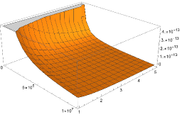
Figure 1: Self-mirror scalar potential $V$ according to $\tau_{0}$ and $\tau_{1}$ with numerical constant value of $W_{0}=1,A_{0}=1,a_{0}=2\pi,b_{0}=1/4,\tau_{1}=10^{7}$. The scalar potential approaches positive value from above at the large volume limit, and therefore de Sitter vacuum approached.

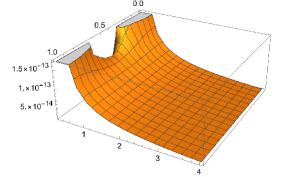
Figure 2: Self-mirror scalar potential at the large volume limit according to $\tau_{0}$ and axionic field $b_{0}=[0,1]$. Here the value $W_{0}=1,A_{0}=1,a_{0}=2\pi,\tau_{1}=10^{7},\tau_{2}=10^{7}$ are used. The positive uplift term at $a_{0}\tau_{0}\sim\ln\mathcal{V}$ provides de Sitter vacuum around the saddle point region.

Large Volume Limit II

In the large volume limit $\mathcal{V}\to\infty$ with $\tau_{0}\to\infty$ exponentially, the non-perturbative superpotential terms approach

$$W=W_{0}+A_{1}e^{-a_{1}T_{1}}+A_{2}e^{-a_{2}T_{2}}.$$ (35)

The effective scalar potential (25), with inverse of Kähler metric element $G^{i\bar{j}}$ ($i,j=1,2$) from (26), become

$$V =\frac{W_{0}^{2}\tau_{0}^{6}}{17496~{}\mathcal{V}^{6}}-\frac{W_{0}^{2}(\tau_{1}+\tau_{2})\tau_{0}^{5}}{2187~{}\mathcal{V}^{6}}$$

$$-\frac{\left(a_{1}A_{1}e^{-a_{1}\tau_{1}}\cos(a_{1}b_{1})+a_{2}A_{2}e^{-a_{2}\tau_{2}}\cos(a_{2}b_{2})\right)W_{0}\tau_{0}^{7}}{104976~{}\mathcal{V}^{6}}$$

$$+\frac{\left(a_{1}^{2}A_{1}^{2}e^{-2a_{1}\tau_{1}}+a_{2}^{2}A_{2}^{2}e^{-2a_{2}\tau_{2}}\right)\tau_{0}^{8}}{1889568~{}\mathcal{V}^{6}}$$

$$+\frac{\left(a_{1}A_{1}a_{2}A_{2}e^{-a_{1}\tau_{1}-a_{2}\tau_{2}}\cos(a_{1}b_{1}-a_{2}b_{2})\right)\tau_{0}^{8}}{1889568~{}\mathcal{V}^{6}}.$$

The total volume of quotient Schoen Calabi-Yau (12) in the large volume limit approaches

$$\mathcal{V}={1\over 18}\sqrt{\tau_{0}(\tau_{0}-6\tau_{1})(\tau_{0}-6\tau_{2})}$$

$$~{}\sim{1\over 18}~{}\tau_{0}^{{3\over 2}},~{}~{}\text{with}~{}\tau_{0}\sim(18\mathcal{V})^{2\over 3},$$ (37)

and therefore the effective scalar potential reduces to

$$V =\frac{36W_{0}^{2}}{\mathcal{V}^{2}}-\frac{8(\frac{2}{3})^{1/3}W_{0}^{2}(\tau_{1}+\tau_{2})}{\mathcal{V}^{8/3}}$$

$$-\frac{2^{2/3}3^{4/3}\left(a_{1}A_{1}e^{-a_{1}\tau_{1}}\cos(a_{1}b_{1})+a_{2}A_{2}e^{-a_{2}\tau_{2}}\cos(a_{2}b_{2})\right)W_{0}}{\mathcal{V}^{4/3}}$$

$$+\frac{2^{1/3}3^{2/3}\left(a_{1}^{2}A_{1}^{2}e^{-2a_{1}\tau_{1}}+a_{2}^{2}A_{2}^{2}e^{-2a_{2}\tau_{2}}\right)}{\mathcal{V}^{2/3}}$$

$$+\frac{2^{1/3}3^{2/3}\left(a_{1}A_{1}a_{2}A_{2}e^{-a_{1}\tau_{1}-a_{2}\tau_{2}}\cos(a_{1}b_{1}-a_{2}b_{2})\right)}{\mathcal{V}^{2/3}}.$$

By taking the decompactification limit for fiber divisor

$$a_{1}\tau_{1}=\ln\mathcal{V},~{}a_{2}\tau_{2}=\ln\mathcal{V},$$ (39)

the effective scalar potential then reduces to

$$V =\frac{36W_{0}^{2}}{\mathcal{V}^{2}}-\frac{8(\frac{2}{3})^{1/3}W_{0}^{2}(\tau_{1}+\tau_{2})}{\mathcal{V}^{8/3}}$$

$$-\frac{2^{2/3}3^{4/3}\left(a_{1}A_{1}\cos(a_{1}b_{1})+a_{2}A_{2}\cos(a_{2}b_{2})\right)W_{0}}{\mathcal{V}^{7/3}}$$

$$+\frac{2^{1/3}3^{2/3}\left(a_{1}^{2}A_{1}^{2}+a_{2}^{2}A_{2}^{2}+a_{1}A_{1}a_{2}A_{2}\cos(a_{1}b_{1}-a_{2}b_{2})\right)}{\mathcal{V}^{8/3}}.$$

In the large volume limit, the leading term $36W_{0}^{2}\over\mathcal{V}^{2}$ takes the dominant value which is obviously positive in the order of $\mathcal{O}(\frac{1}{\mathcal{V}^{2}})$, while the subleading terms suppressed at the order of $\mathcal{O}(\frac{1}{\mathcal{V}^{7/3}})$ and $\mathcal{O}(\frac{1}{\mathcal{V}^{8/3}})$ respectively. Therefore, in total, the non-perturbative scalar potential contributes a positive value, while $W_{0}$ represents the value of the superpotential integrated out from the complex structures and axio-dilatons. Again regard the scalar potential (IV) as $V=V(\mathcal{V},\tau_{1},\tau_{2})$, the possible minimum shall be solved at

$$\frac{\partial V}{\partial\mathcal{V}}=\frac{\partial V}{\partial\tau_{1}}=\frac{\partial V}{\partial\tau_{2}}=0.$$ (41)

From the symmetric construction of volume form with $\tau_{1}$ and $\tau_{2}$, one can solve $\mathcal{V}$ with the value of $\mathcal{V}^{2/3}$ results in

$$\frac{2^{1/3}3^{2/3}W_{0}(a_{1}^{2}A_{1}x\cos(a_{1}b_{1})-a_{2}^{2}A_{2}y\cos(a_{2}b_{2}))}{2a_{1}^{3}A_{1}^{2}x^{2}-2a_{2}^{3}A_{2}^{2}y^{2}+(a_{1}-a_{2})a_{1}A_{1}a_{2}A_{2}xy\cos(a_{1}b_{1}-a_{2}b_{2})},$$ (42)

where $x:=e^{-a_{1}\tau_{1}},~{}y:=e^{-a_{2}\tau_{2}}$. Conveniently, by further taking the decompactification limit $a_{1}A_{1}=W_{0},\,a_{2}A_{2}=W_{0}$, the scalar potential results in the structure

$$V =\frac{36W_{0}^{2}}{\mathcal{V}^{2}}-\frac{\kappa(\tau_{1}+\tau_{2})}{\mathcal{V}^{8/3}}$$

$$-\frac{\lambda(e^{-a_{1}\tau_{1}}\cos(a_{1}b_{1})+e^{-a_{2}\tau_{2}}\cos(a_{2}b_{2}))}{\mathcal{V}^{4/3}}$$

$$+\frac{\mu(e^{-2a_{1}\tau_{1}}+e^{-2a_{2}\tau_{2}}+e^{-a_{1}\tau_{1}-a_{2}\tau_{2}}\cos(a_{1}b_{1}-a_{2}b_{2})}{\mathcal{V}^{2/3}},$$

while $\kappa=8(\frac{2}{3})^{1/3}W_{0}^{2}$, $\lambda=2^{2/3}3^{4/3}W_{0}^{2}$, $\mu=2^{1/3}3^{2/3}W_{0}^{2}$. The value of $\tau_{1},\tau_{2}$ may be further solved with the relation of $y$ and $x$,

$$y=-\frac{\kappa+2\mu a_{1}x^{2}\mathcal{V}^{2}-\lambda a_{1}\cos(a_{1}b_{1})x\mathcal{V}^{4/3}}{\mu a_{1}\cos(a_{1}b_{1}-a_{2}b_{2})x\mathcal{V}^{2}},$$ (44)

as illustrated in Figure 3, where the uplift term takes the dominant effect and essentially gives rise to de Sitter vacua with swampland conjectures criteria satisfied [31].

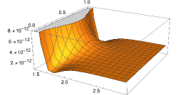
Figure 3: Self-mirror scalar potential of quotient Schoen Calabi-Yau, at the large volume limit $\tau_{0}\to\infty$, $a_{1}\tau_{1},a_{2}\tau_{2}\sim\ln\mathcal{V}$, as function $\tau_{2}$ and axionic field $b_{2}=[0,1]$ according to (IV). Here the value $W_{0}=1,A_{1}=1,A_{2}=1,a_{1}=2\pi,a_{2}=2\pi,\tau_{0}=10^{5},\tau_{1}=2,b_{1}=1/2$ are used. The positive uplift term gives rise to de Sitter vacuum along the $\tau_{1},\tau_{2}$ directions around the saddle point region as illustrated.

V Conclusion

The self-mirror large volume scenario from quotient Schoen Calabi-Yau compactification gave rise to a special uplift term to the effective scalar potential from non-perturbative contribution. This uplift term is intriguingly positive in order $\mathcal{O}(\frac{1}{\mathcal{V}^{2}})$ and essentially lead to de Sitter vacua. In precise, these non-perturbative leading terms $W_{0}^{2}\over\mathcal{V}^{2}$ and $36W_{0}^{2}\over\mathcal{V}^{2}$ became the dominant contribution from large volume scenario, while the contributions from complex structures and axio-dilaton are flux stabilized and integrated out to $W_{0}$ at the vacuum. In particular, the special uplift term is in the same order as from F-term $\frac{DW.DW}{\mathcal{V}^{2}}$ and KKLT mechanism in $\mathcal{O}(\frac{1}{\mathcal{V}^{2}})$. Considering that the special uplift term arises from self-mirror large volume scenario, we propose a new mechanism to obtain de Sitter vacuum.

Acknowledgements: We would in particular like to thank Ralph Blumenhagen, Fernando Quevedo, Jie Zhou for many helpful comments, and thank Michele Cicoli, Wolfgang Lerche, Andre Lukas, Dieter Lüst, Pramod Shukla for helpful discussions. We would also like to thank Xin Gao, Chuying Wang, Xin Wang, Shing Tung Yau and Piljin Yi for helpful discussions on related topics. RS is supported by KIAS New Generation Research Grant PG080701, PG080704, and acknowledge Ludwig Maximilian University of Munich, Max Planck Institute of Physics for their hospitality, and LMU-China Academic Network for their support when this research was initialized.

References

- Balasubramanian et al. [2005] V. Balasubramanian, P. Berglund, J. P. Conlon, and F. Quevedo, Systematics of moduli stabilisation in Calabi-Yau flux compactifications, JHEP 03, 007, arXiv:hep-th/0502058 .
- Conlon et al. [2005] J. P. Conlon, F. Quevedo, and K. Suruliz, Large-volume flux compactifications: Moduli spectrum and D3/D7 soft supersymmetry breaking, JHEP 08, 007, arXiv:hep-th/0505076 .
- Hull [2005] C. M. Hull, A Geometry for non-geometric string backgrounds, JHEP 10, 065, arXiv:hep-th/0406102 .
- Hull and Reid-Edwards [2009] C. M. Hull and R. A. Reid-Edwards, Flux compactifications of string theory on twisted tori, Fortsch. Phys. 57, 862 (2009), arXiv:hep-th/0503114 .
- Shelton et al. [2005] J. Shelton, W. Taylor, and B. Wecht, Nongeometric flux compactifications, JHEP 10, 085, arXiv:hep-th/0508133 .
- Reid-Edwards [2008] R. A. Reid-Edwards, Geometric and non-geometric compactifications of IIB supergravity, JHEP 12, 043, arXiv:hep-th/0610263 .
- Shelton et al. [2007] J. Shelton, W. Taylor, and B. Wecht, Generalized Flux Vacua, JHEP 02, 095, arXiv:hep-th/0607015 .
- Ihl et al. [2007] M. Ihl, D. Robbins, and T. Wrase, Toroidal orientifolds in IIA with general NS-NS fluxes, JHEP 08, 043, arXiv:0705.3410 [hep-th] .
- Marchesano and Schulgin [2007] F. Marchesano and W. Schulgin, Non-geometric fluxes as supergravity backgrounds, Phys. Rev. D 76, 041901 (2007), arXiv:0704.3272 [hep-th] .
- Aldazabal et al. [2006] G. Aldazabal, P. G. Camara, A. Font, and L. E. Ibanez, More dual fluxes and moduli fixing, JHEP 05, 070, arXiv:hep-th/0602089 .
- Grana et al. [2007] M. Grana, J. Louis, and D. Waldram, SU(3) SU(3) compactification and mirror duals of magnetic fluxes, JHEP 04, 101, arXiv:hep-th/0612237 .
- Grana et al. [2009] M. Grana, R. Minasian, M. Petrini, and D. Waldram, T-duality, Generalized Geometry and Non-Geometric Backgrounds, JHEP 04, 075, arXiv:0807.4527 [hep-th] .
- García-Etxebarria et al. [2017] I. n. García-Etxebarria, D. Lust, S. Massai, and C. Mayrhofer, Ubiquity of non-geometry in heterotic compactifications, JHEP 03, 046, arXiv:1611.10291 [hep-th] .
- Blumenhagen et al. [2015] R. Blumenhagen, A. Font, and E. Plauschinn, Relating double field theory to the scalar potential of N = 2 gauged supergravity, JHEP 12, 122, arXiv:1507.08059 [hep-th] .
- Blumenhagen et al. [2016] R. Blumenhagen, C. Damian, A. Font, D. Herschmann, and R. Sun, The Flux-Scaling Scenario: De Sitter Uplift and Axion Inflation, Fortsch. Phys. 64, 536 (2016), arXiv:1510.01522 [hep-th] .
- Note [1] Here we thank Liam Macalister for raising up this problem of non-geometric large volume scenario.
- Curio and Lust [1997] G. Curio and D. Lust, A Class of N=1 dual string pairs and its modular superpotential, Int. J. Mod. Phys. A 12, 5847 (1997), arXiv:hep-th/9703007 .
- Curio and Lust [1998] G. Curio and D. Lust, New N=1 supersymmetric three-dimensional superstring vacua from U manifolds, Phys. Lett. B 428, 95 (1998), arXiv:hep-th/9802193 .
- Schoen [1988] C. Schoen, On fiber products of rational elliptic surfaces with section, Math. Z. 197, 177 (1988).
- Braun et al. [2008] V. Braun, T. Brelidze, M. R. Douglas, and B. A. Ovrut, Calabi-Yau Metrics for Quotients and Complete Intersections, JHEP 05, 080, arXiv:0712.3563 [hep-th] .
- Braun et al. [2004] V. Braun, B. A. Ovrut, T. Pantev, and R. Reinbacher, Elliptic Calabi-Yau threefolds with Z(3) x Z(3) Wilson lines, JHEP 12, 062, arXiv:hep-th/0410055 .
- Braun et al. [2006a] V. Braun, Y.-H. He, B. A. Ovrut, and T. Pantev, Vector bundle extensions, sheaf cohomology, and the heterotic standard model, Adv. Theor. Math. Phys. 10, 525 (2006a), arXiv:hep-th/0505041 .
- Braun et al. [2005] V. Braun, Y.-H. He, B. A. Ovrut, and T. Pantev, A Heterotic standard model, Phys. Lett. B 618, 252 (2005), arXiv:hep-th/0501070 .
- Braun et al. [2006b] V. Braun, Y.-H. He, B. A. Ovrut, and T. Pantev, The Exact MSSM spectrum from string theory, JHEP 05, 043, arXiv:hep-th/0512177 .
- Donagi et al. [2001] R. Donagi, B. A. Ovrut, T. Pantev, and D. Waldram, Standard model bundles on nonsimply connected Calabi-Yau threefolds, JHEP 08, 053, arXiv:hep-th/0008008 .
- Ovrut [2018] B. A. Ovrut, Vacuum Constraints for Realistic Strongly Coupled Heterotic M-Theories, Symmetry 10, 723 (2018), arXiv:1811.08892 [hep-th] .
- Candelas and Davies [2010] P. Candelas and R. Davies, New Calabi-Yau Manifolds with Small Hodge Numbers, Fortsch. Phys. 58, 383 (2010), arXiv:0809.4681 [hep-th] .
- Braun et al. [2010] V. Braun, P. Candelas, and R. Davies, A Three-Generation Calabi-Yau Manifold with Small Hodge Numbers, Fortsch. Phys. 58, 467 (2010), arXiv:0910.5464 [hep-th] .
- Lee et al. [2022] S.-J. Lee, W. Lerche, and T. Weigand, Emergent strings from infinite distance limits, JHEP 02, 190, arXiv:1910.01135 [hep-th] .
- Hull et al. [2017] C. Hull, D. Israel, and A. Sarti, Non-geometric Calabi-Yau Backgrounds and K3 automorphisms, JHEP 11, 084, arXiv:1710.00853 [hep-th] .
- Sun [2024] R. Sun, Large Volume Scenario from Schoen Manifold with de Sitter under Swampland Conjecture, (2024), arXiv:2402.04089 [hep-th] .
- Ovrut et al. [2003] B. A. Ovrut, T. Pantev, and R. Reinbacher, Torus fibered Calabi-Yau threefolds with nontrivial fundamental group, JHEP 05, 040, arXiv:hep-th/0212221 .
- Braun et al. [2007a] V. Braun, M. Kreuzer, B. A. Ovrut, and E. Scheidegger, Worldsheet instantons and torsion curves, part A: Direct computation, JHEP 10, 022, arXiv:hep-th/0703182 .
- Braun et al. [2007b] V. Braun, M. Kreuzer, B. A. Ovrut, and E. Scheidegger, Worldsheet Instantons and Torsion Curves, Part B: Mirror Symmetry, JHEP 10, 023, arXiv:0704.0449 [hep-th] .
- Braun et al. [2007c] V. Braun, M. Kreuzer, B. A. Ovrut, and E. Scheidegger, Worldsheet instantons, torsion curves, and non-perturbative superpotentials, Phys. Lett. B 649, 334 (2007c), arXiv:hep-th/0703134 .
- Witten [1996] E. Witten, Nonperturbative superpotentials in string theory, Nucl. Phys. B 474, 343 (1996), arXiv:hep-th/9604030 .
- Gukov et al. [2000] S. Gukov, C. Vafa, and E. Witten, CFT’s from Calabi-Yau four folds, Nucl. Phys. B 584, 69 (2000), [Erratum: Nucl.Phys.B 608, 477–478 (2001)], arXiv:hep-th/9906070 .