Scalarized Hybrid Neutron Stars in Scalar Tensor Gravity

Abstract

Hybrid neutron stars, the compact objects consisting hadronic matter and strange quark matter, can be considered as the probes for the scalar tensor gravity. In this work, we explore the scalarization of hybrid neutron stars in the scalar tensor gravity. For the hadronic phase, we apply a piecewise polytropic equation of state constrained by the observational data of GW170817 and the data of six low-mass X-ray binaries with thermonuclear burst or the symmetry energy of the nuclear interaction. In addition, to describe the strange quark matter inside the hybrid neutron star, different MIT bag models are employed. We study the effects of the value of bag constant, the mass of s quark, the perturbative quantum chromodynamics correction parameter, and the density jump at the surface of quark-hadronic phase transition on the scalarization of hybrid neutron stars. Our results confirm that the scalarization is more sensitive to the value of bag constant, the mass of s quark, and the density jump compared to the perturbative quantum chromodynamics correction parameter.

I INTRODUCTION

In hybrid neutron stars (HNSs), the remnants of massive stars, the nucleons get decomposed into quarks and therefore form deconfined strange quark matter. Quantum chromodynamics (QCD) explains such phase transition from baryonic to deconfined quark matter at ultra-high densities Alford . The strange quark matter in these stars is surrounded by hadronic matter. With slow conversion speed at the interface, a new class of dynamically stable HNSs can be exist arXiv:2106.10380 . Weakening the deconfinement phase transition leads to axions stabilizes massive HNSs against gravitational collapse arXiv:2206.01631 . HNSs can experience two phase transitions from hadronic matter to low- and high-density quark matter phases arXiv:2301.10940 . The stars with sufficient amount of strange quark matter in the core can convert into the strange quark stars arXiv:2305.01246 . No core singularity in the formations of the HNS can be found arXiv:2307.11809 .

Astrophysical observations are in agreement with the results for the HNSs within the MIT bag model arXiv:2107.08971 , QCD motivated chiral approach arXiv:1411.2856 , vector bag model arXiv:2303.06387 , self-consistent Nambu-Jona-Lasinio model arXiv:1403.7492 ; arXiv:1511.08561 ; arXiv:1703.01431 ; arXiv:1804.10785 ; arXiv:2004.07909 ; arXiv:2104.01519 , and Field Correlator Method arXiv:1909.08661 . In Dyson-Schwinger quark model, HNS mass and radius are affected by the quark-gluon vertex and gluon propagator arXiv:1503.02795 . Considering Nambu-Jona-Lasinio model for HNSs, the vector-isovector terms lead to larger quark cores and smaller deconfinement density arXiv:1610.06435 . Astrophysical data verify the high values of the bag parameter in MIT bag model for HNSs arXiv:2210.09077 . Bag pressure in MIT bag model has important influence in the emergence of the special points in mass radius relation of HNSs arXiv:2303.04653 . HNSs can be self-bound rather than gravitationally bound arXiv:2104.01519 . The strength of the vector interaction affects the equation of state (EoS) of HNS matter and vector strength results in the stiffness of the EoS arXiv:2112.09595 ; arXiv:2305.01662 . The matter in the intermediate density range is expected to be soft, while it is stiff in higher density range arXiv:2303.06387 . The quark-hadron density jump and the EoS determine the crust-breaking frequency and maximum fiducial ellipticity of HNSs arXiv:2210.14048 .

Contribution of HNS quark core is more related to the radius compared to the star mass which is affected by the EoS of the quark matter arXiv:2004.07909 . Exothermic phase transition in cold neutron stars can lead to HNSs with masses smaller than a parent neutron star arXiv:2012.04212 . The mass and tidal deformability constraints from the observational data are in agreement with large strangeness content and large quark cores for HNSs in binary systems arXiv:2105.06239 . Radii of HNSs can constrain the symmetry energy arXiv:2202.11463 . Besides, the maximum masses of HNSs constrain the EoS of symmetric nuclear and quark matter arXiv:2202.11463 . The dark matter in HNSs alters the energy density discontinuity and results in the decrease of the star minimum mass arXiv:2212.12615 . Besides, it affects the star mass radius relation as well as the core radius of the star arXiv:2212.12615 ; fuzzy . Hybrid equations of state describing the quark matter inner core and the nuclear outer core can lead to star with mass of $M=0.77^{+0.20}_{-0.17}M_{\bigodot}$ and radius of $R=10.4^{+0.86}_{-0.78}km$ unlike the nuclear models arXiv:2302.02989 . Lower transition energy density, smaller energy density discontinuity, and higher sound speed of quark matter lead to supermassive HNSs arXiv:2308.06993 .

In relativistic stars, the tachyonic instability as a result of the scalar field and curvature nonminimal coupling results in the spontaneous scalarization. X-Ray and gravitational-wave observations of neutron stars can constrain the massive scalar tensor theories arXiv:2109.13453 . Applying Bayesian analysis, the spontaneous scalarization parameters have been constrained using the neutron star mass and radius measurements arXiv:2204.02138 . Employing the parameters in accordance with the observational data, the scalarization results in significant deviations from the general relativistic universal relations of neutron stars arXiv:1812.00347 . The scalar field in neutron stars affects the pulse profile’s overall shape leading to strong deviations from the General Relativity (GR) one arXiv:1808.04391 . Mutual interplay between magnetic and scalar fields has influence on the magnetic and the scalarisation properties of neutron stars arXiv:2005.12758 . Spontaneous scalarisation alters the neutron star magnetic deformation and emitted quadrupolar gravitational waves arXiv:2010.14833 .

Scalar field in neutron stars is suppressed due to the self-interaction in scalar tensor theory arXiv:1805.07818 . Topological neutron stars in tensor-multi-scalar theories of gravity are characterized by topological charge arXiv:1911.06908 . In scalar tensor theories, a quasi-universal relation between the scalar charge and stellar binding energy has been presented arXiv:2105.01614 . Scalar-gauge coupling in Einstein gravity induces spontaneous scalarization in charged stars arXiv:2105.14661 . The scalar field couplings to Ricci scalar and Gauss-Bonnet invariant affect the domain of existence and the amount of scalar charge in scalarized neutron stars arXiv:2111.03644 .

The neutron star maximum compactness in GR is larger than the one in scalar tensor gravity arXiv:1806.00568 . In mixed configurations of tensor-multi-scalar solitons and relativistic neutron stars, the stability region extends over larger central energy densities and central values of the scalar field arXiv:1909.00473 . In tensor-multi-scalar theories of gravity, a family of scalarized branches specified by the number of the scalar field nodes appears and separates from the general relativistic solution at the points with new unstable modes arXiv:2004.03956 . Nonscalarized stars can convert to scalarized ones through the core collapse arXiv:2103.11999 . Neutron stars in degenerate higher-order scalar tensor theories have masses and radii larger than the ones in GR arXiv:2207.13624 . In this work, we investigate the properties of scalarized HNSs. In section II, the EoSs which describe the HNSs are presented. Section III is related to scalar tensor theory. The structure of scalarized HNSs is explained in section IV. Section V is devoted to conclusion.

II Hybrid Neutron Star Equation of State

In this paper, we utilize a model for HNS similar the one described in Ref. Pereira et al. (2021) . The HNS includes a quark core and a hadronic layer. In this model, we suppose that a sharp phase transition surface without a mixed phase divides two parts and the density can be discontinuous at the phase splitting surface Pereira et al.2020 . For the hadronic phase, we employ the dense neutron star matter EoS in the form of a piecewise polytropic expansion constrained by the observational data related to GW170817 as well as the data of six low-mass X-ray binaries with thermonuclear burst or the symmetry energy of the nuclear interaction Jiang et al.2019 . In order to describe the quark core, we apply different MIT bag models including massless quark approximation Banerjee21 , massive strange quark matter considering the QCD coupling constant Farhi ; Zdunik ; 0901.1268 , and interacting strange quark matter specified by effective bag constant and perturbative QCD corrections term Farhi . These models for the quark phase will be described in the following. We take the density jump at the quark-hadronic phase transition surface as a free parameter. This jump is described by the parameter $\eta$ defined as

$$\eta\equiv\frac{\epsilon_{q}}{\epsilon_{h}}-1,$$ (1)

with the density at the top of the quark phase, $\epsilon_{q}$, and the density at the bottom of the hadronic phase, $\epsilon_{h}$. We can calculate $\epsilon_{q}$ or $\epsilon_{h}$ and the pressure at the phase transition surface using $p_{q}=p_{h}$ at the phase transition surface.

In the massless quark approximation, a system containing $u$, $d$, and $s$ quarks that are noninteracting and massless is considered. Applying this approximation in MIT bag model, the quark pressure $P$ takes the following form

$$P=\frac{1}{3}(\epsilon-4B),$$ (2)

in which $\epsilon$ denotes the energy density of the quark matter distribution and $B$ presents the bag constant that acts as the inward pressure appropriate to confine quarks inside the bag. Fig. 1 shows the EoS of HNS in the massless quark approximation with different values of the bag constant $B$ and the density jump $\eta$. We have assumed $\rho_{0}=1.66\times 10^{14}g/cm^{3}$. The pressure takes higher values as the density jump increases, especially at lower densities. The pressure decreases as the bag constant increases from $B=70MeV/fm^{3}$ to $B=75MeV/fm^{3}$.

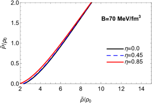
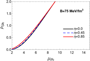
Figure 1: EoS of HNS in the massless quark approximation considering different values of the bag constant, $B$, and the density jump, $\eta$.

The second MIT bag model that we employ in this work is the massive strange quark matter considering the QCD coupling constant. In this model, the quark matter is composed of the massless $u$ and $d$ quarks, electrons $e$, and massive $s$ quarks Farhi . The EoS of quark matter in this system depends on the bag constant, $B$, the QCD coupling constant, $\alpha_{c}$, the mass of the strange quark, $m_{s}$, and the renormalization point, $\rho_{N}$. We select the values $\rho_{N}=313MeV$ similar to Ref. Farhi and $\alpha_{c}=0.2$ following Ref. 0901.1268 . In Fig. 2, we have presented the EoS of HNS considering the massive strange quark matter with the QCD coupling constant. With lower values of the bag constant and the strange quark mass, the effect of the density jump on the EoS is more significant. Besides, the EoS is softer considering higher values of the bag constant and the strange quark mass.

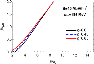
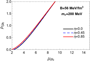
Figure 2: EoS of HNS considering the massive strange quark matter with the QCD coupling constant. Different values of the bag constant, $B$, the mass of the strange quark, $m_{s}$, and the density jump, $\eta$, have been applied.

In the third model, the interacting strange quark matter characterized by the effective bag constant and the perturbative QCD corrections term is explored. For this model, a mixture of quarks, $u$, $d$, $s$, and electrons $e$, with the transformation due to weak interaction between quarks and leptons is considered Farhi . The grand canonical potential per unit volume is given by

$$\Omega=\sum_{i=u,d,s,e}\Omega_{i}^{0}+\frac{3(1-a_{4})}{4\pi^{2}}\mu^{4}+B_{eff}.$$ (3)

In the above equation, the grand canonical potential for $u$, $d$, $s$ quarks and electrons as the ideal relativistic Fermi gases is presented by $\Omega_{i}^{0}$. Besides, the average quark chemical potential is denoted by $\mu=(\mu_{u}+\mu_{d}+\mu_{s})/3$. We present the contributions from the QCD vacuum using $B_{eff}$ and the perturbative QCD contribution from one-gluon exchange for gluon interaction by $a_{4}$. The number density of particles in strange quark matter is written as

$$n_{i}=-\frac{\partial\Omega}{\partial\mu_{i}},$$ (4)

in which $\mu_{i}(i=u,d,s,e)$ is the chemical potential of particles. The weak interactions determine the conditions for the quark matter at the equilibrium state,

$$\mu_{d}=\mu_{u}+\mu_{e},$$ (5)

$$\mu_{d}=\mu_{s}.$$ (6)

The charge neutrality condition is also given by

$$\frac{2}{3}n_{u}=\frac{1}{3}[n_{d}+n_{s}]+n_{e}.$$ (7)

The pressure of quark matter is then as follows

$$P=-\Omega,$$ (8)

and the energy density is given by

$$\varepsilon=\Omega+\sum_{i=u,d,s,e}\mu_{i}n_{i}.$$ (9)

Fig. 3 shows the EoS of HNS in the third model with different values of $B_{eff}$ and $a_{4}$. We have fixed the strange quark mass $m_{s}=100\ MeV$ and the density jump $\eta=0$. The pressure decreases by increasing the effective bag constant. The influence of the effective bag constant is more significant at higher densities. In this paper, we investigate the scalarized HNSs which described by the above EoSs.

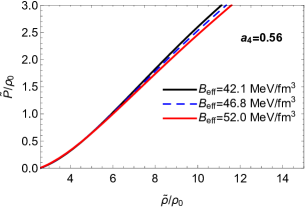
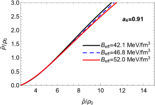
Figure 3: EoS of HNS in the third model considering different values of $B_{eff}$ and $a_{4}$ with fixed values of the strange quark mass $m_{s}=100\ MeV$ and the density jump $\eta=0$.

III Scalar Tensor gravity

Scalar tensor theories in Einstein frame can be defined by the following action

$$S[g_{\mu\nu},\phi,\Psi_{m}]=\frac{1}{16\pi}\int d^{4}x\sqrt{-g}(R-2\nabla_{\mu}\phi\nabla^{\mu}\phi)+S_{m}[\Psi_{m},a(\phi)^{2}g_{\mu\nu}].$$ (10)

In the above equation, $g=det(g_{\mu\nu})$, $R$ is Ricci scalar, $\phi$ shows the scalar field, $\Psi_{m}$ denotes the matter field, and $a(\phi)$ is the coupling function satisfying the relation $\tilde{g}_{\mu\nu}=a(\phi)g_{\mu\nu}$ between $g_{\mu\nu}$ in Einstein frame and $\tilde{g_{\mu\nu}}$ in Jordan frame. Here, we assume the form of the coupling function as $a(\phi)=e^{\frac{1}{2}\beta(\phi-\phi_{0})^{2}}$ with the coupling constant $\beta$ and $\phi_{0}=0$. To describe a spherical symmetric static HNS in the scalar tensor theory in Einstein frame, we apply the following form of the spacetime line element

$$ds^{2}=-N(r)^{2}dt^{2}+A(r)^{2}dr^{2}+r^{2}(d\theta^{2}+\sin^{2}\theta d\phi^{2}),$$ (11)

with the metric functions $N(r)$ and $A(r)=[1-2m(r)/r]^{-1/2}$ and the mass profile $m(r)$. Therefore, the field equations result in the following differential equations [28],

$$\frac{dm}{dr}=4\pi r^{2}a^{4}\tilde{\epsilon}+\frac{r}{2}(r-2m)\Big{(}\frac{d\phi}{dr}\Big{)}^{2},$$ (12)

$$\frac{d\ln N}{dr}=\frac{4\pi r^{2}a^{4}\tilde{p}}{r-2m}+\frac{r}{2}\Big{(}\frac{d\phi}{dr}\Big{)}^{2}+\frac{m}{r(r-2m)},$$ (13)

$$\frac{d^{2}\phi}{dr^{2}}=\frac{4\pi ra^{4}}{r-2m}\!\left[\alpha(\tilde{\epsilon}-3\tilde{p})+r(\tilde{\epsilon}-\tilde{p})\frac{d\phi}{dr}\right]\!-\frac{2(r-m)}{r(r-2m)}\frac{d\phi}{dr},$$ (14)

$$\frac{d\tilde{p}}{dr}=-(\tilde{\epsilon}+\tilde{p})\left[\frac{4\pi r^{2}a^{4}\tilde{p}}{r-2m}\!+\!\frac{r}{2}\Big{(}\frac{d\phi}{dr}\Big{)}^{2}\!\!+\!\frac{m}{r(r-2m)}\!+\!\alpha\frac{d\phi}{dr}\right],$$ (15)

$$\frac{dm_{b}}{dr}=\frac{4\pi r^{2}a^{3}\tilde{\rho}}{\sqrt{1-\frac{2m}{r}}}.$$ (16)

Here, $\tilde{\epsilon}$ is the energy density, $\tilde{p}$ shows the pressure, and $m_{b}$ denotes the baryonic mass. The boundary conditions which used for solving these equations are

$$m(0)=m_{b}(0)=0,\quad\lim_{r\to\infty}N(r)=1,\quad\phi(0)=\phi_{c},\quad\lim_{r\to\infty}\phi(r)=0,$$

$$\frac{d\phi}{dr}(0)=0,\qquad\tilde{p}(0)=p_{c},\qquad\tilde{p}(R_{s})=0.$$ (17)

Here, the star radius is presented by $R_{s}$ and $c$ shows the center of star. Considering an appropriate boundary conditions at $r=0$ as well as a guess $\phi(0)=\phi_{c}$ at the center, the iteration on $\phi_{c}$ is done getting the condition 26 ; 28 ,

$$\phi_{s}+\frac{2\psi_{s}}{\sqrt{\dot{\nu}_{s}^{2}+4\psi_{s}^{2}}}\textrm{arctanh}\left[\frac{\sqrt{\dot{\nu}_{s}^{2}+4\psi_{s}^{2}}}{\dot{\nu}_{s}+2/R_{s}}\right]=0,$$ (18)

in which s indicates the quantities on the surface of the star as well as $\psi_{s}=(d\phi/dr)_{s}$ and $\dot{\nu}_{s}=2(d\ln N/dr)|_{s}=R_{s}\psi_{s}^{2}+2m_{s}/[R_{s}(R_{s}-2m_{s})]$. The ADM mass, $M_{ADM}$, and the scalar charge, $\omega$, are also calculated as follows [26,28],

$$M_{ADM} =\frac{R_{s}^{2}\dot{\nu}_{s}}{2}\left(1-\frac{2m_{s}}{R_{s}}\right)^{\frac{1}{2}}\exp\left[\frac{-\dot{\nu}_{s}}{\sqrt{\dot{\nu}_{s}^{2}+4\psi_{s}^{2}}}\textrm{arctanh}\left(\frac{\sqrt{\dot{\nu}_{s}^{2}+4\psi_{s}^{2}}}{\dot{\nu}_{s}+2/R_{s}}\right)\right],$$ (19)

$$\omega =-2M_{ADM}\psi_{s}/\dot{\nu}_{s}.$$ (20)

Here, we report the values of the HNS ADM mass. In the following, we study the HNS in the scalar tensor gravity.

IV RESULTS and DISCUSSION

IV.1 Mass of scalarized hybrid neutron star

We have presented the mass of HNS applying different EoS models in Figs. 4-6. Figs. 4 and 5 confirm that with the higher values of the density jump, the star mass grows. This effect becomes more important by increasing $\eta=0.45$ to $\eta=0.85$. Fig. 6 verifies that the star mass reduces as $B_{eff}$ increases. In all cases, the deviation of scalarized star mass from the GR one is more clear with smaller values of $\beta$. The range of star mass at which the HNS is scalarized becomes larger by decreasing the coupling constant. Applying three models for the HNS EoS, the most massive stars are the scalarized ones. With lower values of $\beta$, the maximum star mass grows. The central densities corresponding to most massive scalarized stars decrease as the density jump increases. Our results show that considering the higher values of the bag constant leads to the scalarization of the HNSs with larger central densities (see Figs. 4 and 5). It is obvious from Fig. 6 that the most massive stars in the third model are the scalarized ones with lower values of $B_{eff}$ and $\beta$. Besides, the central density related to the maximum mass of scalarized stars in the third model increases by $B_{eff}$.

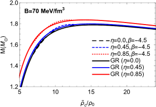
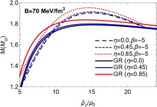
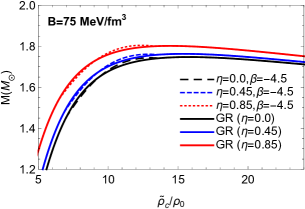
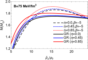
Figure 4: HNS mass in the first model for the HNS EoS applying the scalar tensor gravity and GR. Different values of the bag constant, $B$, the density jump, $\eta$, and the coupling constant, $\beta$, have been considered.

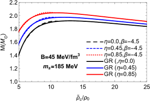
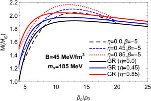
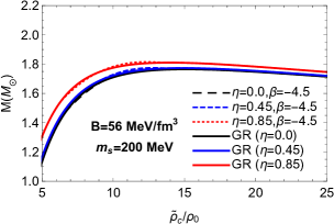
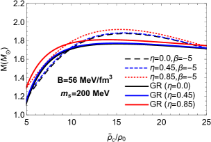
Figure 5: Same as Fig. 4 but for the second model of the HNS EoS. We have applied different values of the bag constant, $B$, the mass of the strange quark, $m_{s}$, and the density jump, $\eta$.

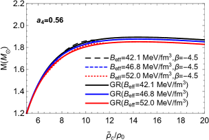
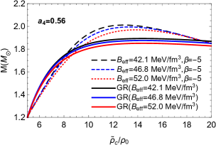
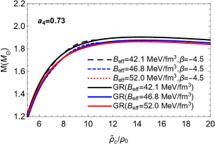
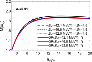
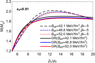
Figure 6: Same as Fig. 4 but for the third model of the HNS EoS. Different values of $B_{eff}$ and $a_{4}$ with fixed values of the strange quark mass, $m_{s}=100\ MeV$, and the density jump, $\eta=0$, have been considered.

In Tables 1-3, the maximum mass of HNS considering different models for the HNS EoS employing the scalar tensor gravity and GR is presented. These tables confirm that the maximum mass of scalarized stars with $\beta=-4.5$ is almost equal to the GR one. Besides, for both scalarized stars and the stars in GR, the maximum mass decreases by increasing the coupling constant. Table 2 shows that in the second model, the maximum mass decreases by increasing the bag constant and the mass of the strange quark. In addition, it is obvious from Table 3 that the maximum mass of HNS is not significantly affected by the model parameter $a_{4}$.

		$B=70MeV/fm^{3}$			$B=75MeV/fm^{3}$
$\beta$	$\eta=0$	$\eta=0.45$	$\eta=0.85$	$\eta=0$	$\eta=0.45$	$\eta=0.85$
$-4.5$	1.79	1.80	1.84	1.75	1.76	1.80
$-5$	1.90	1.91	1.95	1.86	1.87	1.91
$GR$	1.79	1.80	1.84	1.75	1.76	1.80

Table 1: Maximum mass (in solar mass unit) of HNS in the first model for the HNS EoS with different values of the bag constant, $B$, the density jump, $\eta$, and the coupling constant, $\beta$.

		$B=45MeV/fm^{3}$			$B=56MeV/fm^{3}$
		$m_{s}=185MeV$			$m_{s}=200MeV$
$\beta$	$\eta=0$	$\eta=0.45$	$\eta=0.85$	$\eta=0$	$\eta=0.45$	$\eta=0.85$
$-4.5$	1.92	1.98	2.05	1.76	1.77	1.82
$-5$	2.04	2.10	2.17	1.88	1.88	1.92
$GR$	1.92	1.98	2.04	1.76	1.77	1.81

Table 2: Same as Table 1 but for the second model of the HNS EoS.

			$a_{4}=0.56$			$a_{4}=0.73$			$a_{4}=0.91$
	$B_{eff}(\frac{MeV}{fm^{3}})$	$42.1$	$46.8$	$52.0$	$42.1$	$46.8$	$52.0$	$42.1$	$46.8$	$52.0$
$\beta$
$-4.5$		1.89	1.88	1.85	1.90	1.88	1.86	1.90	1.87	1.86
$-5$		2.01	1.99	1.97	2.02	1.99	1.98	2.02	1.99	1.98
$GR$		1.89	1.88	1.85	1.90	1.88	1.86	1.90	1.87	1.86

Table 3: Same as Table 1 but for the third model of the HNS EoS.

IV.2 Central scalar field in hybrid neutron star

Figs. 7-9 demonstrate the central scalar field in HNS employing different models for the HNS EoS. The coupling constant affects the spontaneous scalarization with higher values of the central scalar field considering the lower values of the coupling constant. The range of the central density at which the central scalar field is nonzero becomes larger applying the smaller values of $\beta$. Figs. 7 and 8 verify that the central density at which $\phi_{c}$ becomes nonzero (first critical density) decreases as the density jump in HNS grows. The central density at which the spontaneous scalarization terminates, i.e. $\phi_{c}=0$, (second critical density) is also smaller when the density jump is larger. Fig. 9 shows that the effective bag constant alters the spontaneous scalarization. Our calculations indicate that the second critical density grows by increasing the effective bag constant, while the first one is not almost affected by the effective bag constant. The increase of the second critical density by $B_{eff}$ is more important when the coupling constant is smaller. In the third model of the HNS EoS, with higher values of the effective bag constant, the range of the scalarization increases. In all cases, the reduction of the coupling constant leads to the decrement in the first critical density and increment in the second one.

Tables 4-6 give the first critical density of the spontaneous scalarization for different models of the HNS EoS. Table 4 confirms that in the first model of the HNS EoS, the first critical density grows as the bag constant increases. This is also true for the second critical density, with higher values of the second critical density by increasing the bag constant (see Fig. 7). It is clear from Table 5 that in the second model of the HNS EoS, the first critical density grows as the bag constant and the mass of the strange quark increase. This enhancement also takes place for the second critical density (see Fig. 8). Our results show that the effects of the bag constant and the mass of the strange quark on the spontaneous scalarization are more remarkable when the density jump in HNS is larger. Table 6 approves that the influence of the effective bag constant as well as the model parameter $a_{4}$ on the first critical density is nearly negligible. Fig. 10 presents the critical value of the coupling constant, $\beta_{cr}$, at which the spontaneous scalarization takes place. It is obvious that this critical value is nearly the same in different models of the HNS EoS, i.e. the value $\beta_{cr}\simeq-4.35$.

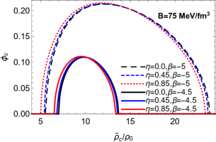
Figure 7: Central scalar field, $\phi_{c}$, versus the central density, $\rho_{c}$, applying first model of the HNS EoS with different values of the bag constant, $B$, the density jump, $\eta$, and the coupling constant, $\beta$.

$\beta$	$\eta$	$B=70MeV/fm^{3}$	$B=75MeV/fm^{3}$
	$0$	6.7	7.1
$-4.5$	$0.45$	6.6	6.9
	$0.85$	6.3	6.6
	$0$	5.4	5.6
$-5$	$0.45$	5.3	5.5
	$0.85$	5	5.1

Table 4: First critical density (in unit of $\rho_{0}$) of the spontaneous scalarization in the first model of the HNS EoS.

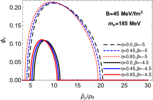
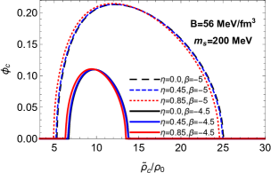
Figure 8: Same as Fig. 7 but for the second model of the HNS EoS considering different values of the bag constant, $B$, the mass of the strange quark, $m_{s}$, and the density jump, $\eta$.

$\beta$	$\eta$	$B=45MeV/fm^{3}$	$B=56MeV/fm^{3}$
		$m_{s}=185MeV$	$m_{s}=200MeV$
	$0$	6.4	6.8
$-4.5$	$0.45$	5.4	6.7
	$0.85$	5	6.4
	$0$	4.7	5.4
$-5$	$0.45$	4.3	5.3
	$0.85$	3.9	5

Table 5: Same as Table 4 but for the second model of the HNS EoS.

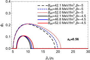
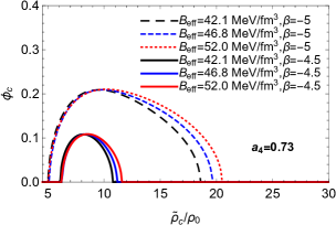
Figure 9: Same as Fig. 7 but for the third model of the HNS EoS applying different values of $B_{eff}$ and $a_{4}$ with fixed values of the strange quark mass, $m_{s}=100\ MeV$, and the density jump, $\eta=0$.

$\beta$	$B_{eff}(MeV/fm^{3})$	$a_{4}=0.56$	$a_{4}=0.73$	$a_{4}=0.91$
	$42.1$	6.2	6.2	6.2
$-4.5$	$46.8$	6.3	6.3	6.3
	$52.0$	6.3	6.3	6.3
	$42.1$	5.1	5.1	5.1
$-0.5$	$46.8$	5.1	5.2	5.2
	$52.0$	5.2	5.1	5.1

Table 6: Same as Table 4 but for the third model of the HNS EoS.

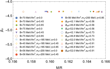
Figure 10: Critical value of the coupling constant, $\beta_{cr}$, versus the star compactness, $M/R$, in different models of the HNS EoS considered in this paper.

IV.3 Hybrid neutron star scalar charge

In Figs. 11-13, we have plotted the scalar charge of HNS in different models of the HNS EoS. Scalar charge of scalarized HNS increases by decreasing the coupling constant. With higher values of the density jump, the scalar charge is larger. Considering the stars with larger $\eta$, the less values of the compactness are needed for appearance of the scalar charge (Figs. 11 and 12). Fig. 12 confirms that in the second model of the HNS EoS, the scalar charge reduces when the bag constant and the mass of the strange quark become larger. Besides, applying the lower values of the bag constant and the mass of the strange quark, the influences of the density jump on the scalar charge are more significant. Fig. 13 confirms that with the lower values of the coupling constant, the effective bag constant alters the scalar charge more significantly.

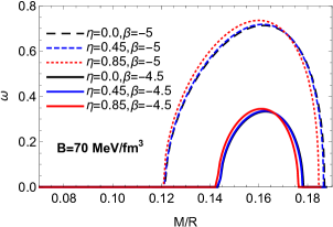
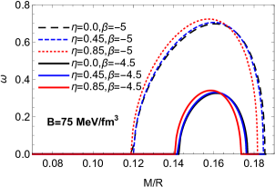
Figure 11: Scalar charge of HNS, $\omega$, versus the star compactness, $M/R$, in the first model of the HNS EoS with different values of the bag constant, $B$, the density jump, $\eta$, and the coupling constant, $\beta$.

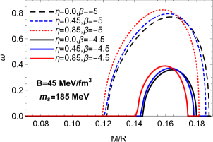
Figure 12: Same as Fig. 11 but in the second model of the HNS EoS with different values of the bag constant, $B$, the mass of the strange quark, $m_{s}$, and the density jump, $\eta$.

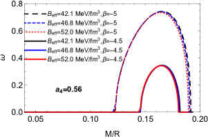
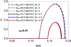
Figure 13: Same as Fig. 11 but in the third model of the HNS EoS applying different values of $B_{eff}$ and $a_{4}$ with fixed values of the strange quark mass, $m_{s}=100\ MeV$, and the density jump, $\eta=0$.

V SUMMARY AND CONCLUDING REMARKS

In the present work, we have studied the hybrid neutron stars (HNSs) in the scalar tensor gravity. For this aim, a piecewise polytropic EoS constrained by the observational data and different MIT bag models have been employed to describe the hadronic phase and the strange quark matter, respectively. Our calculations approve that the density jump in the HNS affects the central density of most massive scalarized stars. The effective bag constant alters the mass of scalarized stars as well as the central density corresponding to the maximum mass. In addition, the density jump in HNS leads to the reduction of the first and the second critical densities of the spontaneous scalarization. However, the second critical density increases as the effective bag constant grows. The range of the HNS scalarization becomes larger by increasing the effective bag constant. Besides, the scalar charge of HNS grows as the density jump increases.

- (1) M. G. Alford, S. Han, and K. Schwenzer, J. Phys. G, Nucl. Part. Phys. 46, 114001 (2019).
- (2) G. Lugones, M. Mariani, and I. F. Ranea-Sandoval, J. Cosmol. Astropart. Phys. 03, 028 (2023).
- (3) B. S. Lopes, R. L. S. Farias, V. Dexheimer, A. Bandyopadhyay, and R. O. Ramos, Phys. Rev. D 106, L121301 (2022).
- (4) J. J. Li, A. Sedrakian, and M. Alford, Astrophys. J. 944, 206 (2023).
- (5) H. Liu, Y. -H. Yang, Y. Han, and P. -C. Chu, Phys. Rev. D 108, 034004 (2023).
- (6) P. Bhar, S. Pradhan, A. Malik, and P. K. Sahoo, Eur. Phys. J. C 83, 646 (2023).
- (7) D. Sen, N. Alam, and G. Chaudhuri, J. Phys. G, Nucl. Part. Phys. 48, 105201 (2021).
- (8) S. Benic, D. Blaschke, D. E. Alvarez-Castillo, T. Fischer, and S. Typel, Astron. Astrophys. 577, A40 (2015).
- (9) A. Kumar, V. B. Thapa, and M. Sinha, Phys. Rev. D 107, 063024 (2023).
- (10) N. Yasutake, R. Lastowiecki, S. Benic, D. Blaschke, T. Maruyama, and T. Tatsumi, Phys. Rev. C 89, 065803 (2014).
- (11) D. L. Whittenbury, H. H. Matevosyan, and A. W. Thomas, Phys. Rev. C 93, 035807 (2016).
- (12) C. -M. Li, J. -L. Zhang, T. Zhao, Y. -P. Zhao, and H. -S. Zong, Phys. Rev. D 95, 056018 (2017).
- (13) C. -M. Li, J. -L. Zhang, Y. Yan, Y. -F. Huang, H. -S. Zong, Phys. Rev. D 97, 103013 (2018).
- (14) L. L. Lopes and D. P. Menezes, Nucl. Phys. A 1009, 122171 (2021).
- (15) L. -Q. Su, C. Shi, Y. -F. Huang, Y. Yan, C. -M. Li, and H. Zong, Phys. Rev. D 103, 094037 (2021).
- (16) M. Mariani, M. G. Orsaria, I. F. Ranea-Sandoval, and G. Lugones, Mon. Not. R. Astron. Soc. 489, 4261 (2019).
- (17) H. Chen, J. -B. Wei, M. Baldo, G. F. Burgio, and H. -J. Schulze, Phys. Rev. D 91, 105002 (2015).
- (18) R. C. Pereira, P. Costa, and C. Providencia, Phys. Rev. D 94, 094001 (2016).
- (19) S. Shirke, S. Ghosh, and D. Chatterjee, Astrophys. J. 944, 7 (2023).
- (20) S. Pal, S. Podder, D. Sen, and G. Chaudhuri, Phys. Rev. D 107, 063019 (2023).
- (21) A. Pfaff, H. Hansen, and F. Gulminelli, Phys. Rev. C 105, 035802 (2022).
- (22) H. Liu, X. -M. Zhang, and P. -C. Chu, Phys. Rev. D 107, 094032 (2023).
- (23) J. P. Pereira, M. Bejger, P. Haensel, and J. L. Zdunik, Astrophys. J. 950, 185 (2023).
- (24) R. Mallick, S. Singh, and R. Nandi, Mon. Not. R. Astron. Soc. 503, 4829 (2021).
- (25) M. Ferreira, R. C. Pereira, and C. Providencia, Phys. Rev. D 103, 123020 (2021).
- (26) H. Liu, J. Xu, and P. -C. Chu, Phys. Rev. D 105, 043015 (2022).
- (27) C. H. Lenzi, M. Dutra, O. Lourenco, L. L. Lopes, and D. P. Menezes, Eur. Phys. J. C 83, 266 (2023).
- (28) Z. Rezaei, Mon. Not. R. Astron. Soc. 524, 2015 (2023).
- (29) L. Brodie and A. Haber, Phys. Rev. C 108, 025806 (2023).
- (30) H. Sun and D. Wen, Phys. Rev. C 108, 025801 (2023).
- (31) Z. Hu, Y. Gao, R. Xu, and L. Shao, Phys. Rev. D 104, 104014 (2021).
- (32) S. Tuna, K. I. Unluturk, and F. M. Ramazanoglu, Phys. Rev. D 105, 124070 (2022).
- (33) D. Popchev, K. V. Staykov, D. D. Doneva, and S. S. Yazadjiev, Eur. Phys. J. C 79, 178 (2019).
- (34) H. O. Silva and N. Yunes, Phys. Rev. D 99, 044034 (2019).
- (35) J. Soldateschi, N. Bucciantini, and L. D. Zanna, Astron. Astrophys. 640, A44 (2020).
- (36) J. Soldateschi, N. Bucciantini, and L. D. Zanna, Astron. Astrophys. 645, A39 (2021).
- (37) K. V. Staykov, D. Popchev, D. D. Doneva, and S. S. Yazadjiev, Eur. Phys. J. C 78, 586 (2018).
- (38) D. D. Doneva and S. S. Yazadjiev, Phys. Rev. D 101, 064072 (2020).
- (39) K. Yagi and M. Stepniczka, Phys. Rev. D 104, 044017 (2021).
- (40) M. Minamitsuji and S. Tsujikawa, Phys. Lett. B 820, 136509 (2021).
- (41) G. Ventagli, G. Antoniou, A. Lehebel, and T. P. Sotiriou, Phys. Rev. D 104, 124078 (2021).
- (42) H. Sotani and K. D. Kokkotas, Phys. Rev. D 97, 124034 (2018).
- (43) D. D. Doneva and S. S. Yazadjiev, Phys. Rev. D 101, 024009 (2020).
- (44) D. D. Doneva and S. S. Yazadjiev, Phys. Rev. D 101, 104010 (2020).
- (45) H. -J. Kuan, D. D. Doneva, and S. S. Yazadjiev, Phys. Rev. Lett. 127, 161103 (2021).
- (46) H. Boumaza and D. Langlois, Phys. Rev. D 106, 084053 (2022).
- (47) J. P. Pereira et al., Astrophys. J. 910, 145 (2021).
- (48) J. P. Pereira, M. Bejger, N. Andersson, F. Gittins, Astrophys. J. 895, 28 (2020).
- (49) J. -L. Jiang et al., Astrophys. J. 885, 39 (2019).
- (50) A. Banerjee, T. Tangphati, and P. Channuie, Astrophys. J. 909, 14 (2021).
- (51) E. Farhi and R. L. Jaffe, Phys. Rev. D 30, 2379 (1984).
- (52) J. L. Zdunik, Astron. Astrophys. 359, 311 (2000).
- (53) P. Haensel, J. L. Zdunik, M. Bejger, J. M. Lattimer, Astron. Astrophys. 502, 605 (2009).
- (54) T. Damour and G. Esposito-Farese, Phys. Rev. Lett. 70, 2220 (1993).
- (55) R. F. P. Mendes and N. Ortiz, Phys. Rev. D 93, 124035 (2016).