Interleaving One-Class and Weakly-Supervised Models with Adaptive Thresholding for Unsupervised Video Anomaly Detection

Abstract

Without human annotations, a typical Unsupervised Video Anomaly Detection (UVAD) method needs to train two models that generate pseudo labels for each other. In previous work, the two models are closely entangled with each other, and it is not known how to upgrade their method without modifying their training framework significantly. Second, previous work usually adopts fixed thresholding to obtain pseudo labels, however the user-specified threshold is not reliable which inevitably introduces errors into the training process. To alleviate these two problems, we propose a novel interleaved framework that alternately trains a One-Class Classification (OCC) model and a Weakly-Supervised (WS) model for UVAD. The OCC or WS models in our method can be easily replaced with other OCC or WS models, which facilitates our method to upgrade with the most recent developments in both fields. For handling the fixed thresholding problem, we break through the conventional cognitive boundary and propose a weighted OCC model that can be trained on both normal and abnormal data. We also propose an adaptive mechanism for automatically finding the optimal threshold for the WS model in a loose to strict manner. Experiments demonstrate that the proposed UVAD method outperforms previous approaches.

1 Introduction

Video Anomaly Detection (VAD) is a task that identifies abnormal events in a video, where the abnormal event could be a fire alarm, a flaw in an industrial product, or a traffic accident, etc. Most previous VAD methods can be classified into two categories: One-Class Classification (OCC) methods [22, 21, 13, 59, 5, 17, 28, 29, 31, 37, 53, 39, 52, 42, 30, 35, 45, 11, 3, 44, 23, 34, 4, 27, 46, 58] and Weakly-Supervised (WS) approaches [38, 2, 7, 57, 43, 49, 25, 56, 33, 8, 20, 60, 50]. OCC methods are trained only on normal data to establish the normal distribution. Any data that deviates from the normal distribution is deemed as abnormal at test time [22, 21, 13, 59]. In comparison, WS approaches require video-level labels that indicate a video is normal (no abnormal event occurs in the video) or abnormal (there is at least one abnormal event).

As opposed to the abundant works in the field of supervised approaches (including OCC and WS approaches), there is much less effort made for devising purely unsupervised VAD methods [55]. Many previous works [16, 13] refer to OCC models as unsupervised approaches, but strictly they are not as the training data that they rely on are manually labeled as normal. In this paper, we attempt to tackle the purely Unsupervised VAD (UVAD) task not requiring any human annotated label, which not only saves human labor but also makes it possible to leverage the tremendous surveillance videos captured by CCTV cameras every day.

UVAD is extremely challenging due to the absence of supervisory signals, and there is rare work on tackling this challenge despite its potential applications. As far as we know, the work of [55] is the first UVAD method. It trains two VAD models, including an OCC model and a binary classification model, to generate pseudo labels for training each other. However, the method suffers from two problems. First, at the very beginning of their design, the two models are closely entangled together in a cooperative learning framework. Specifically, the OCC model, which is an AutoEncoder (AE) that reconstructs video features, is of low ability to recognize abnormal events, which greatly limits the performance of this UVAD method. It is not easy to upgrade the AE model to other OCC models, otherwise one may need to change the binary classifier model too as it shares the same data organization scheme with the AE model. Second, the method adopts fixed thresholding mechanisms to annotate events into pseudo labels, but the thresholds are specified by the user manually, which are not accurate and may inject errors into the training process.

In this paper, we propose a novel framework that interleaves an OCC method and a WS method with adaptive thresholding for UVAD. As there is only a weak connection between the OCC and WS model, we argue that any OCC or WS models are suitable for our well-designed interleaved framework. This property makes our method able to instantly leverage the latest development in the two mainstream VAD fields. More importantly, in our framework, we extend the current OCC models that must be trained on normal data to a weighted OCC paradigm that can be trained on both normal and abnormal data, totally avoiding the necessity of thresholding for the OCC model. On the other hand, we propose an adaptive thresholding mechanism in a loose to strict manner, which finds the most appropriate threshold for the WS model automatically. Armed with the state-of-the-art OCC and WS models, and also solving the error-prone fixed thresholding problem, we achieve a very effective UVAD method that is even competitive with the supervised counterparts.

In summary, the main contributions of this work include:

• We propose a novel interleaved UVAD framework that alternately runs OCC and WS VAD models, which does not rely on fixed thresholding for generating binary labels.

• We proposed a weighted OCC model to train on both normal and abnormal data, avoiding the thresholding to specify the normal data for the OCC model training.

• For the WS model, we propose an inner-outer-loop UVAD framework within which we progressively tighten the threshold of the WS model and find the most appropriate threshold during this process.

• Experiments show that our UVAD method outperforms the previous UVAD method and also the variants of our method with fixed thresholds. Our UVAD framework can degenerate into a supervised OCC or WS method. The degenerated models are highly competitive among existing OCC and WS approaches.

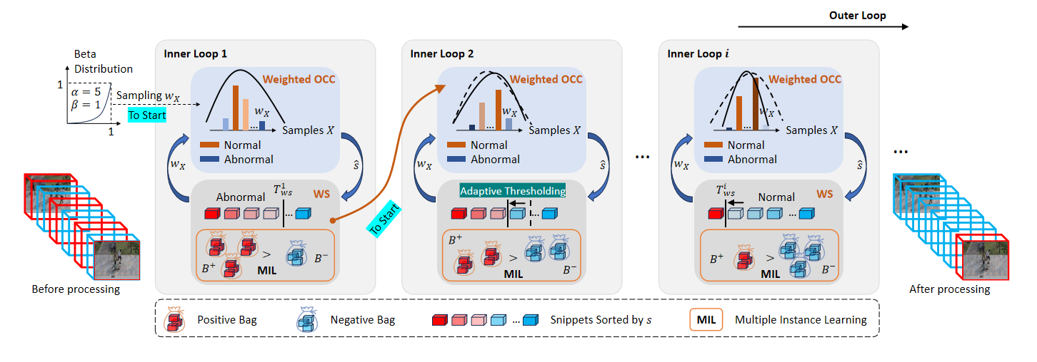
Figure 1: Pipeline of our proposed interleaved framework. The basic building block is an “inner loop” in which we alternately run a weighted OCC model and a WS model. The weighted OCC model is trained on both normal and abnormal samples by leveraging the importance weight $w_{X}$ assigned to each training sample. The WS model is trained in the multiple instance learning (MIL) framework on positive/negative bags $B^{+}$/$B^{-}$ composed of abnormal/normal snippets. Labels of snippets are obtained by thresholding the sorted snippets according to their anomaly scores $\hat{s}$, with threshold $T_{ws}$. The OCC model provides the WS model with $\hat{s}$, and the WS model provides the OCC model with $w_{X}$. To adaptively adjust $T_{ws}$, our method contains many inner loops. After one inner loop converges, we use a loose to strict method to update the threshold $T_{ws}$, and use the new threshold in the next inner loop. To start the first inner loop, we randomly sample $w_{X}$ to train the OCC model. All the other inner loops are started by using the last WS model in the previous inner loop to supply $w_{X}$. Before processing, most of the events are wrongly classified, while after processing we obtain accurate VAD results.

2 Related Work

One-Class Classification VAD (OCC). OCC-based VAD approaches only have access to normal data and try to model normal data to identify behaviors that are significantly different from normal behaviors as anomalies. Early works use hand-crafted features to help detect anomalies [4, 27, 46, 58]. With the rapid development of deep learning, recent methods turn to normal representations extracted by using a deep neural network [42, 30, 35, 45]. Some methods recognize normal patterns by using the reconstruction/prediction model to reconstruct the representations [22, 21, 13, 59, 5, 17, 28, 29, 31, 37, 53, 39, 52]. These models may lead to well-reconstructed anomalies, thereby limiting the performance of the OCC-based methods. Therefore, other OCC-based methods turn to identify normal representations by using proxy tasks [11, 3, 44, 23, 34]. What’s more, recently, Hirschorn and Avidan [16] propose to build a multivariate Gaussian distribution for normal data and detect instances deviating from this distribution as anomalies. However, the above methods treat all samples equally, ignoring the potential differences in importance between normal samples.

Weakly-Supervised VAD (WS). In weakly-supervised VAD, video-level annotations are available in the training stage. Sultani et al [38] first propose to use the video-level labels and solve WS VAD based on multi-instance learning (MIL) framework [2, 7]. Since then, many works [57, 43, 49, 25, 56, 33] have viewed the WS VAD task as a MIL problem. Tian et al. [40] develop to extend MIL to Top-$k$ MIL method by training with a robust temporal feature magnitude (RTFM) loss function. The methods mentioned above directly train in the supervision of video-level labels and the coarse-grained supervision limits the accuracy of WS models. Recently, two-stage self-training methods [8, 20, 60, 50] adopt a two-stage pipeline to use more fine-grained labels to supervise the networks more strictly. The WS model in our framework shares a similar idea with [8] and is tailored to use finer-grained snippet-level labels.

Unsupervised VAD (UVAD). Unsupervised VAD requires identifying anomalies from data containing both normal and abnormal samples without any annotation. This is a challenging new task that is almost unexplored in the literature. Although significant progress has been made in OCC and WS VAD, directly applying them independently to address UVAD does not yield good results. Zaheer et al. [55] firstly raise this task and propose to solve UVAD by generative cooperative learning (GCL). According to  [55], an important attribute of the training set is that normal events are more frequent than abnormal events. Utilizing the attribute, our proposed method modifies both the OCC and WS VAD models and combines the modified two models together to learn from unmarked training data.

Adaptive Thresholding in Deep Learning. Semi/un-supervised learning approaches [12, 6] trained on massive unlabeled data usually identify the classes of unlabeled data by thresholding the model’s confidence [51, 32]. Samples determined by the model to have a probability of belonging to a particular category above the corresponding threshold can be labeled as such and added to subsequent training. Sohn et al. [36] propose to use a fixed strict threshold to determine the high-quality pseudo labels. Guo and Li [14] further propose to obtain adaptive thresholds for each class from a pre-defined threshold. Recently, Wang et al. [47] develop a self-adaptive manner to adjust the threshold of each class. The above methods usually assume there is a small amount of label data, while we employ an adaptive thresholding to divide abnormal and normal data without any annotation prior.

3 Our Method

As shown in Figure 1, the core of our method is a pair of OCC and WS VAD models trained alternately while providing pseudo labels for each other (the inner loop). The two models are connected only by the pseudo labels. Any model that can provide such labels in that format can be used in our method. Another point is that, previously, the pseudo labels are 0 and 1 binary labels which are obtained by a thresholding method with fixed thresholds. The main contribution of this paper is to avoid the thresholding needed conventionally or compute the threshold automatically.

3.1 Interleave OCC and WS Training UVAD

Denote by $\mathcal{V}=\{V_{1},V_{2},\cdots,V_{i},\cdots\}$ a set of videos without normal or abnormal labels. We would like to train an OCC model and a WS model on these videos. For the OCC model, we extract a set of objects $\mathcal{X}=\{X_{1},X_{2},\cdots,X_{i},\cdots\}$ from the training videos, where $X_{i}$ can be a video snippet [55], a spatiotemporal cube cropped out of a video [22], or a sequence of poses of a person [16], etc. Each object $X_{i}$ is the basic building block processed by the OCC model. Note that the size of the set $\mathcal{V}$ and $\mathcal{X}$ are different, and the size of $\mathcal{X}$ is much larger than that of $\mathcal{V}$. For the WS model, we split training videos into snippets, obtaining a set of snippets $\mathcal{S}=\{S_{1},S_{2},\cdots,S_{i},\cdots\}$. Each snippet $S_{i}$ is the basic element processed by the WS model.

Conventionally, to train the OCC model, we need to prepare a set of pseudo labels

$$l_{\mathcal{X}}=\{l_{X_{1}},l_{X_{2}},\cdots,l_{X_{i}},\cdots\}$$ (1)

for the corresponding objects in $\mathcal{X}$, where $l_{X_{i}}\in\{0,1\}$ is the label of $X_{i}$ which is abnormal if $l_{X_{i}}$ is 1 and normal otherwise. Similarly, to train the WS model, we need to prepare a set of pseudo labels

$$l_{\mathcal{S}}=\{l_{S_{1}},l_{S_{2}},\cdots,l_{S_{i}},\cdots,\}$$ (2)

with $l_{S_{i}}\in\{0,1\}$ being the label of snippet $S_{i}$.

OCC Model and Pseudo Labels $l_{\mathcal{S}}$. Before, OCC models are deeded as only trained on normal data. This is the source yielding the problem that when we integrate OCC into a UVAD framework we need to identify the normal data in the training dataset. In this paper, we break through this cognitive boundary by extending the conventional OCC paradigm to a weighted one that can be trained on both normal and abnormal data.

Formally, we define $f_{occ}$ as the OCC model and minimize the following weighted negative log-likelihood across all the data:

$$\mathcal{L}_{occ}=-w_{X}log(p_{Z}(f_{occ}(X))),$$ (3)

where $X\in\mathcal{X}$ is sampled from the whole training dataset rather than the normal part, $Z=f_{occ}(X)$ is the feature extracted from $X$ by the model, $p_{Z}$ is the established distribution of the normal data, and $w_{X}\in[0,1]$ is the weight of the object $X$ indicating the normality degree of the object. With this new formulation, all the training data are taken into consideration when training the OCC model, avoiding the thresholding that distinguishes normal data from abnormal data. Objects with larger $w_{X}$ are better captured by the learned distribution of the OCC model, while others are not. The weighted OCC model adjusts itself to match with the importance of each training object $X$. In practice, we compute $w_{X}$ by:

$$w_{X}=1-\hat{x},$$ (4)

where $\hat{x}$ is the anomaly score of object $X$ computed by the WS model which ranges $[0,1]$.

Assuming the above weighted OCC model is trained, and let $x_{i}=p_{Z}(f_{occ}(X_{i}))$ be the anomaly score of the object $X_{i}$ computed by the OCC model. We can compute the anomaly score $\hat{s}_{i}$ of a video snippet $S_{i}$ by averaging all the anomaly scores of objects occurring in the snippet. Then, the pseudo labels for the WS model provided by OCC can be determined by the following thresholding:

$$l_{S_{i}}=\begin{cases}1,\quad{\rm if}\quad{\rm Rank}(\hat{s}_{i})<T_{ws},\\ 0,\quad{\rm otherwise},\end{cases}$$ (5)

where ${\rm Rank(\cdot)}$ sorts the snippets by their anomaly scores in descending order and returns the index of $S_{i}$ among all the snippets, and $T_{ws}$ is the threshold.

WS Model and Pseudo Labels $w_{X}$ (not $l_{\mathcal{X}}$). With snippet-level pseudo annotations $L_{\mathcal{S}}$ (obtained in Eq. 5), we randomly select $C=16$ abnormal snippets to compose a positive bag $B^{+}=\{S_{i}^{+}\}_{i=1}^{C}$ , and randomly select $C$ normal snippets to compose a negative bag $B^{-}=\{S_{j}^{-}\}_{j=1}^{C}$. Note that previous approaches [38, 40] usually treat snippets of the same video as a bag based on video-level labels. Differently, thanks to the snippet-level labels provided by the OCC model, we can compose positive and negative bags more flexibly. By multiple instance learning, we then train a WS model to ensure the maximum anomaly score in positive bags exceeds that in negative bags:

$$\begin{split}\mathcal{L}_{ws}=\operatorname{max}(0,m-f_{ws}(B^{+})+f_{ws}(B^{-}))+\\ \mathcal{L}_{BCE}(B^{+})+\mathcal{L}_{BCE}(B^{-}),\end{split}$$ (6)

where $f_{ws}$ is the WS model, $m$ is the margin, and $f_{ws}(B)$ (where $B$ can be $B^{+}$ or $B^{-}$) returns the maximum anomaly score of snippets in a bag  [38], or the average of the Top-$k$ maximum magnitudes of features  [40]. Finally,

$$\small\mathcal{L}_{BCE}(B)=-Y\operatorname{log}(f_{ws}(B))+(1-Y)\operatorname{log}(1-f_{ws}(B)),$$ (7)

where $Y$ is the label of the bag $B$.

With the trained WS model, we compute anomaly score $\hat{x}_{i}$ of object $X_{i}$ by simply setting $\hat{x}_{i}$ as the anomaly score of the corresponding snippet containing the object $X_{i}$. Our proposed weighted OCC model does not require binary labels $l_{\mathcal{X}}$ in Eq. 1 any more. Instead, the WS model provides weight $w_{X_{i}}=1-\hat{x}_{i}$ to the weighted OCC model.

Discussion. As seen, the OCC and WS models in our method are weakly connected by pseudo labels. This design allows any OCC or WS model that can provide such labels to be used in our model. We argue that this is an important property of a UVAD method, since the modern OCC and WS methods are quickly developed and it is a natural idea to leverage the developments in the two fields. With our design, we have the flexibility to substitute the OCC/WS model in our framework with other advanced OCC/WS models.

Besides the above flexibility, we also propose the novel weighted OCC paradigm, which is a more comprehensive form eliminating the need to specify the normal data for training.

3.2 Adaptive Thresholding

We have solved the thresholding problem for the OCC model, but we still need to perform thresholding for the WS model defined in Eq.5 as the WS model needs the binary labels to assist the construction of positive and negative bags. However, it is rarely accurate to manually specify the threshold $T_{ws}$. In light of this, we propose a method to find an adaptive threshold in a loose to strict manner.

Our key idea is to first indicate a relatively loose threshold at the very beginning. In this case, more snippets than the actual number are mislabeled as abnormal. Then, we gradually decrease the threshold to make more strict decisions about the abnormal snippets. We believe the actual number of abnormal snippets must exist inbetween the largest and smallest thresholds, and try to find the threshold that approaches the real ratio of abnormal data the most during this threshold annealing process.

To this end, after the alternate training of OCC and WS models converges (which we call an inner loop), we re-run the inner loop again and again, forming our inner-outer-loop UVAD framework (see Figure 1). For the first inner loop, we set $T^{1}_{ws}=R\%\times N$, where for example, $R=30$, and $N$ is the total number of snippets in the training dataset. This setting is very loose, as generally the ratio of abnormal data in a dataset is much less than 30%. In our experiments, we set different $R$ (e.g. from 15% to 35%) and find that it does not influence our final results much, demonstrating the robustness of our method. In any latter inner loop, we use all the trained OCC models in the previous inner loops to determine the threshold. Recall that after each alternate training between OCC and WS models, we obtain a unique OCC model. We use this model to compute snippet anomaly scores, sort the snippets, and use $A_{j}$ to denote the set of the first $R\%$ abnormal snippets identified by the $j^{th}$ unique OCC model. The ranking threshold $T^{i}_{ws}$ used in the $i^{th}$ inner loop is computed as:

$$T^{i}_{ws}={\rm Num}(A_{1}\cap A_{2}\cap\cdots\cap A_{M_{i-1}}),\forall i>1,$$ (8)

where $M_{i-1}$ is the total number of OCC models trained in the loop from 1 to $i-1$, and ${\rm Num}(\cdot)$ counts the number of elements in the intersection set. The size of the intersection set becomes more and more smaller, making the threshold more and more strict. The remaining snippets in the set are of higher confidence being abnormal as more and more voters view them as abnormal.

To elucidate the effect of the above adaptive thresholding method, we visualize how an originally very weak WS model is gradually improved as more inner loops execute in Figure 2. In the figure, we show a video with an abnormal event in the middle. In the first inner loop (with $T_{ws}=1643$), the WS model wrongly identifies the abnormal event to be normal (see curves on the left). After executing more and more inner loops, $T_{ws}$ becomes smaller and smaller (finally reduced to 834 after 5 inner loops), and the WS model begins to identify the anomaly event progressively. Accordingly, the WS model can provide more accurate $w_{X}$ (on the right) for training the OCC model.

Figure 2: As outer loop goes, $T_{ws}$ becomes smaller and smaller, while the WS model is improved gradually. Figures on the left: anomaly score curves of video frames. Right: the corresponding weights supplying for weighted OCC model.

3.3 Alternate Training with Inner-Outer Loops

Weighted OCC training relies on pseudo labels generated by the WS model, and conversely, WS training requires pseudo labels derived from the OCC. This egg and chicken problem needs to be solved at the very beginning in each inner loop. Our solution is to pre-train the OCC model using pseudo labels from some place other than the inner loop.

Starting the Inner Loop. For the first inner loop, we randomly sample the weight $w_{X}\sim{\rm Beta}(\alpha,\beta)$, i.e. sampling $w_{X}$ from the Beta distribution where $\alpha=5$ and $\beta=1$. The sampled weights are mostly around 1, and a small portion of them is close to 0, in line with the usual assumption that the training data contains more normal data and less abnormal data. For other inner loops, its OCC model is pre-trained by $w_{X}$ generated by the final WS model in the last inner loop (see the red arrow in Figure 1). We train the OCC and WS models in a new inner loop from scratch, not inheriting parameters from the last loop.

Inner Loop Convergence Analysis. We analyze the convergence of the inner loop empirically, which is validated by the experiment in Figure 5 . At the very beginning, we randomly initialize the weight $w_{X}$ to train our OCC model. Although the random initialization is not precise, the OCC model can still learn normal patterns from the training data, as we assume there is much more normal data than abnormal data in the training dataset. The OCC model then produces relatively reliable pseudo labels for training the WS model. Very confidently, the WS model can provide better weights to the OCC model than the random initialization, with which we train better OCC model and better WS model alternately, until convergence.

Outer Loop Stopping Criteria. At the very beginning, $T_{ws}$ is larger than the real number of abnormal snippets, then it progressively approaches the real number as the outer loop runs, and finally becomes smaller than the real number due to the set intersection operation. We need to stop the outer loop when $T_{ws}$ approaches the real number the most. We experimentally find that $T_{ws}$ drops very fast at the first a few inner loops, then the rate of change of $T_{ws}$ becomes small which indicates the all the OCCs achieve a consensus about the abnormal snippets and the number of intersection among $\{A_{i}|i=1,\ldots,M_{i-1}\}$ is probably the real number. Based on this consideration, once the quantity of ranking threshold change between two consecutive inner loops is less than $Q\%$ of its first changing quantity, the whole training process is stopped in our method. Please see the high correlation between the change of $T_{ws}$ and the accuracy of the WS model in Figure 3.

3.4 Anomaly Scoring

Since our method is composed of OCC and WS models, we provide both anomaly scores of the two models, when comparing our method with previous OCC and WS models.

4 Experiments

4.1 Datasets and Evaluation Metrics

ShanghaiTech. The ShanghaiTech dataset [21] contains 437 videos and was originally created as a benchmark for OCC with only normal videos available in the training set. Zhong et al. [60] reorganized the dataset to enable the training of WS systems. The new split of the training set contains 63 abnormal videos and 175 normal videos, while there are 44 anomalous and 155 normal videos in the new testing split. In our unsupervised setting, we follow the split for WS approaches but do not provide video-level annotations in the training stage.

UBnormal. The UBnormal dataset [1] is a synthetic supervised open-set benchmark, which contains 268 training videos, 64 validation videos and 211 test videos. Both normal and abnormal videos are mixed in these three kinds of subsets. The dataset is very challenging because of disjoint sets of anomaly types in the training and testing set. We follow its original organization but train our proposed UVAD without any annotations.

Evaluation Metrics. Following prior VAD arts [15, 24, 38, 60], we use the frame-level area under the ROC curve (AUC) to measure the accuracy of VAD for both datasets.

4.2 OCC and WS models Employed

As stated, our method is a flexible UVAD framework that can use different kinds of OCC and WS models. We test using three OCC models, including a simple AutoEncoder (AE) model used in  [55], the Jigsaw method proposed in [44], and STG-NF [16].

(1) AE. GCL [55] propose to use an AutoEncoder that reconstructs the features extracted from videos as their OCC model. The architecture of the AE is FC[2048,1024,512,256,512,1024,2048].

(2) Jigsaw. The OCC model Jigsaw [44] addresses VAD by solving a pretext task: spatio-temporal jigsaw puzzles. It divides the spatio-temporal space of a video into smaller cubes, then shuffles the positions of the cubes, and finally tries to restore the original positions of the cubes.

(3) STG-NF. STG-NF [16] extracts pose sequences of persons, and extends the Glow [19] to build the multivariate Gaussian distribution of normal person action sequences.

For the WS model, we test the method proposed in Sultani et al. [38] and RTFM [40].

(1) Sultani et al. [38]. Sultani et al. [38] propose the first MIL VAD model that maximizes the separability between any a positive bag containing snippets of an abnormal video and a negative bag with snippets of a normal video.

(2) RTFM. RTFM [40] extends Sultani et al. [38] to compare the Top-$k$ largest magnitude snippets between positive and negative bags.

Supervision	Method	Features	STech AUC %	UB AUC %
One-Class Classification	MemAE  [13]	-	71.20	-
	Frame Prediction  [21]	-	73.40	-
	Markovitz et al.  [26]	-	76.10	52.00
	HF2-VAD  [22]	-	76.20	-
	CT-D2GAN  [9]	-	77.70	-
	CAC  [48]	-	79.30	-
	SSMTL  [10]	-	82.40	-
	Georgescu et al.  [11]	-	82.70	59.30
	SSMTL++  [3]	-	83.80	62.10
	Jigsaw  [44]	-	84.30	56.40
	STG-NF  [16]	-	85.90	71.80
	Our${}_{OCC}^{*}$ (STG-NF)	I3D	86.37	72.81
Weakly Supervised	GCN [60]	C3D	76.44	-
	GCN [60]	TSN	84.44	-
	Zhang et al. [57]	C3D	82.50	-
	Sultani et al.  [38]	I3D	84.53	54.12
	AR-Net  [43]	I3D	85.38	-
	CLAWS  [54]	C3D	89.67	-
	MIST  [8]	I3D	94.83	-
	Li et al.  [20]	I3D	96.08	-
	RTFM  [40]	C3D	91.51	62.30
	RTFM  [40]	I3D	96.10	66.83
	S3R  [49]	I3D	97.48	-
	Our${}_{WS}^{*}$ (RTFM)	I3D	96.33	67.42
Unsupervised	AEAllData	I3D	60.51	-
	STG-NFAllData  [16]	-	80.29	70.48
	GCL [55]	I3D	76.14	-
	OurOCC	C3D	81.50	71.67
	OurWS		85.43	59.05
	OurOCC	I3D	82.57	74.76
	OurWS		88.18	63.10

Table 1: Comparison with previous approaches. For OCC, we use STG-NF [16]. For WS, we use RTFM [40]. We test using C3D [41] and I3D [18] to extract features. Our_OCC gives the AUC of the OCC model. Our_WS gives the AUC of the WS model. * means our method degenerated to supervised OCC or WS method.

OCC Model	OurOCC	Our${}_{WS}(RTFM)$	GCLClassifier
AE	70.99	78.90	76.14
Jigsaw [44]	81.23	85.35	-
STG-NF [16]	82.57	88.18	-

Table 2: Ablation study on using different OCC models in our method, always with RTFM as the WS model. Our method with an AE-based OCC model is the most appropriate one to fairly compare with GCL [55] which uses the AE-based OCC too.

4.3 Implementation Details

We implement our method in PyTorch. Both the OCC and WS models are optimized by Adam optimizer with $\beta_{1}=0.9$, $\beta_{2}=0.999$, and a weight decay of 0.0005. The batch size of the OCC model (STG-NF) is 256, and the batch size of the WS model (RTFM) is 32. The learning rate is $5e-4$ and $1e-3$ for the OCC (STG-NF) and WS (RTFM) models respectively. For the WS(RTFM) model, the margin $m$ is set to 100 followed [40]. By default, we alternate training the OCC and WS models for one epoch each. The implementation details for other types of OCC (e.g., AE, Jigsaw) and WS models (Sultani et al. [38]) can be found in the supplemental material.

Besides, our method has two hyperparameters shared by all types of OCC or WS models. One is $R\%$ which determines the initial loose threshold of $T_{ws}$. By default, we set it to 15% for the ShanghaiTech dataset which contains a small ratio of abnormal data. In contrast, the UBnormal dataset contains relatively more abnormal data and we set $R\%$ to $30\%$. The other parameter is $Q\%$ used to stop the outer loop. For both datasets, we set $Q\%$ to 10%.

WS Model	OurOCC (STG-NF)	OurWS
Sultani et al.  [38]	81.92	77.41
RTFM [16]	82.57	88.18

Table 3: Ablation study on using different WS models in our method, always with STG-NF as the OCC model.

Weighted OCC	Adaptive Thresholding	RTFM AUC %	STG-NF AUC %
✗	✗	82.06	80.52
✓	✗	83.48	81.78
✗	✓	85.86	81.94
✓	✓	88.18	82.57

Table 4: Comparison with fixed thresholding. The first row degenerates to the fixed-thresholding version of our method. The following two rows use fixed-threshold for the OCC or WS model separately. The last row shows our method without fixed thresholding.

4.4 Comparison with Previous Approaches

Table 1 shows the comparison between our and previous approaches. Since the unsupervised methods are rare, besides GCL [55], we compare with AE_AllData which means training the AE model on the whole training dataset containing both normal and abnormal data. We also compare with STG-NF_AllData. For our method, we adopt STG-NF [16] as our OCC model, and RTFM [40] as the WS model.

First, Our_OCC (I3D) outperforms STG-NF_AllData. This validates the benefit of using our method to distinguish the normal from abnormal data in the training dataset. On ShanghaiTech, our method improves STG-NF from 80.29% to 82.57%. In contrast, the improvement is from 70.48% to 74.76% on UBnormal. The improvement on UBnormal is larger as there is more abnormal data in UBnormal which causes STG-NF_AllData to perform worse.

Second, please compare our method with GCL. Our_WS achieves an AUC of 88.18%, while that of GCL is 76.14% (this score is reported by the classifier of GCL, thus we use our WS model for the comparison). This significant improvement is partly due to the reason that we use a stronger OCC model, i.e., STG-NF, than GCL. If using the same OCC model, our method outperforms GCL by 2.76%, as shown in Table 2.

Our UVAD method can degenerate into a supervised method. For example, we can train our method on the normal data only (using the GT labels provided by the datasets), obtaining Our${}_{OCC}^{*}$. Our degenerated OCC model outperforms all the existing supervised OCC approaches. This validates the effectiveness of the proposed weighted OCC with weighted importance, as even among the normal data there is data that is more normal than other data.

We also degenerate our method into a WS method by making our WS model know video-level labels. All the snippets of normal videos are treated as normal, while snippets of abnormal videos are processed by our adaptive thresholding approach. As seen, Our${}_{WS}^{*}$ (RTFM) outperforms the baseline RTFM [40] (re-implemented by us). On UBnormal, our method achieves the best results among all the existing WS methods.

4.5 Ablation Study and Discussions

Using Different OCC or WS Models. In Table 2, we conduct experiments of using different types of OCC models in our method. We test AE [55], Jigsaw [44], and STG-NF [16], while always using RTFM [40] as the WS model. As can be seen, the effectiveness of our method is essentially affected by the OCC model. A similar trend is shown in Table 3 where the same OCC model is used but with different WS models. Overall, a better OCC or WS model yields better results. The flexibility of incorporating different types of OCC or WS models is a major advantage of our method compared to previous approaches (e.g. GCL [54]).

Figure 3: Left: results of ShanghaiTech. Right: UBnormal. Top: $T_{ws}$ in each inner loop, which drops as more inner loops execute. Bottom: AUC after each inner loop, which increases at first and then decreases. Stars in the top figures show stopping positions by the criteria where our method just right achieves its best results.

Comparison with Fixed Thresholding. In Table 4, the first row shows results of using fixed thresholding for both OCC and WS models. The second and third rows use fixed thresholding for one of the OCC and WS models. The fourth row shows our method without fixed thresholding. As seen, our method outperforms all the other variants.

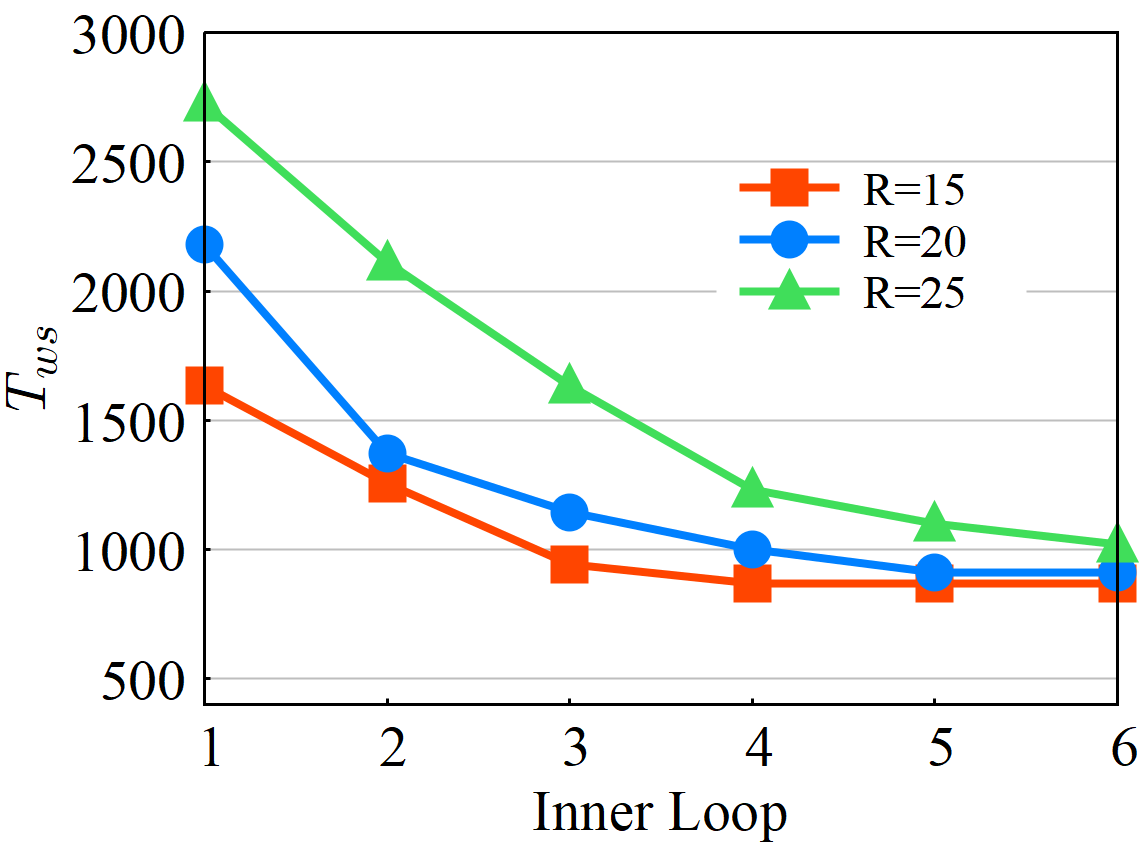
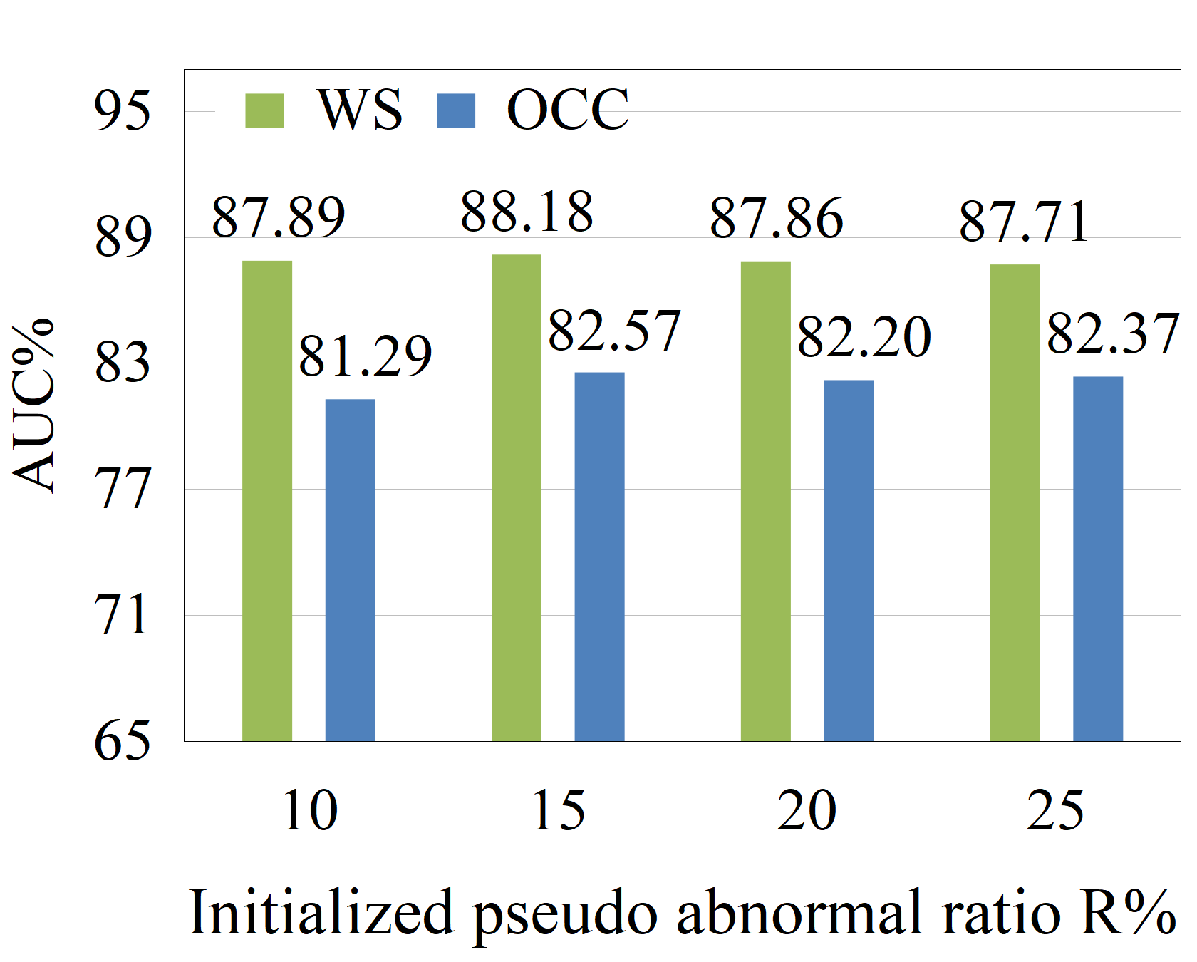
Figure 4: Top: different $R$% converge to similar $T_{ws}$ after 6 inner loops (ShanghaiTech). Bottom left: different $R$% yield similar AUC on ShanghaiTech. Bottom right: different $R$% yield similar AUC on UBnormal.

Effectiveness of the Stopping Criteria. In Figure 3, we show that with the current stopping criteria, our method can stop when it achieves the best AUC (i.e., the best VAD accuracy). Please see that as more inner loops execute, $T_{ws}$ drops and AUC increases. $T_{ws}$ drops very fast at the very beginning, and then the drop rate becomes slower. Simultaneously, AUC first increases and then decreases. We stop our method when the change rate of $T_{ws}$ is about 10% of its original change rate, which finds the best stopping positions as indicated by the stars in the top figures.

Robustness to $R$%. Our method is robust to the initial ratio $R$% of abnormal data specified by the user, as demonstrated in Figure 4. On the top, we show that the threshold $T_{ws}$ converges to similar numbers after 6 inner loops when using different $R$%. At the bottom, we show that different $R$% yield similar AUC on both training datasets. The experiments demonstrate that our method is not influenced much by this parameter for each dataset. However, for different datasets, we need to set different $R$% that roughly match with the anomaly ratio in the datasets.

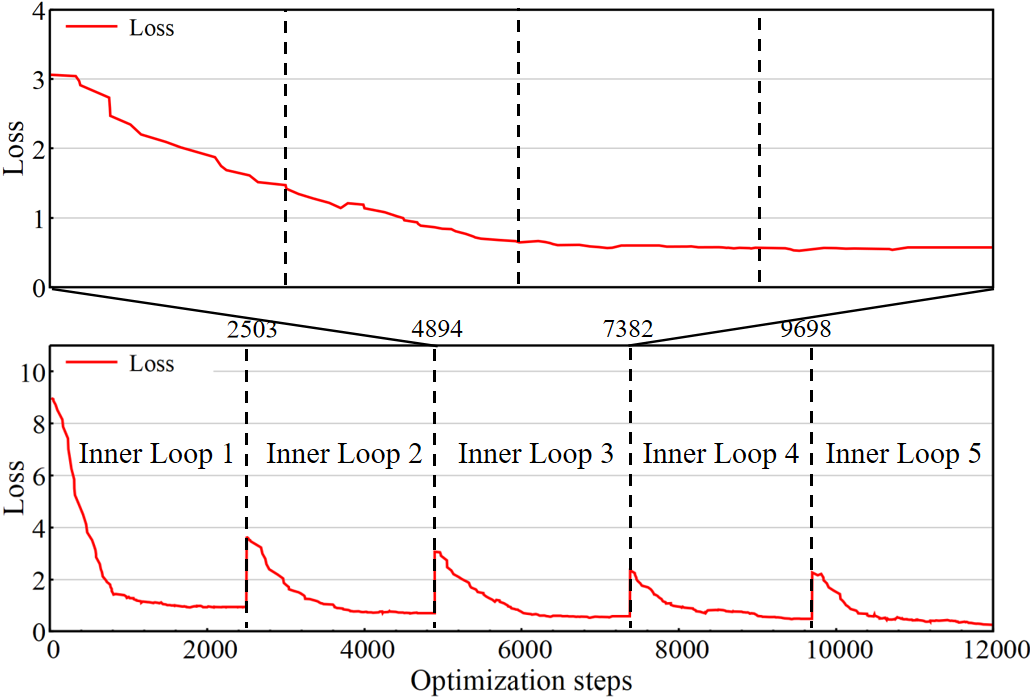
Figure 5: Bottom: training loss curve of the OCC model during the whole training process which decreases steadily with lower and lower peak magnitude as more inner loops execute. Top: zoomed-in training loss curve in the third inner loop.

Training Loss Curve. In Figure 5, we show the training loss curve of the OCC (STG-NF) model in our framework. As seen, the loss drops smoothly in each inner loop. Since we re-train the OCC model from scratch in each loop, the loss suddenly increases at the beginning of the next inner loop, but the peak magnitude of the loss is lower than that of the previous inner loop. Please check the zoomed-in curve showing the loss curve of the OCC model in the third inner loop. The alternate training does not hinder the decline of the loss. The training loss curve of the WS model is put into the supplemental material.

Training Time. Although we need to train the OCC and WS models alternately many times in multiple inner loops, our method is fast in training. That is because, we just train the OCC (or WS) model for one epoch, and then go to optimize the WS (or OCC) model for another epoch. This forms a single training step. Our inner loop converges very fast, containing just a few training steps. As shown in Table 5, there are only 17 training steps during the whole training, yielding a total of 34=2(OCC and WS)$\times$1(epoch)$\times$17(all training steps) epochs. It costs us around 2.5 hours to train our method on ShanghaiTech. We have also trained the OCC or WS model for 2 or 3 epochs in each training step, but obtain worse results while spending more time.

Qualitative Results. To further prove the effectiveness of our framework, we visualize the anomaly scores on ShanghaiTech in Figure 6. As performed in Figure 6(a) and Figure 6(c), the WS and OCC models in our framework reach a consensus and are able to identify the anomalous area in abnormal videos. Figure 6(b) and Figure 6(d) shows the results of both models on a normal video. More results can be found in the supplemental material.

5 Conclusion

In this paper, we propose to interleave the One-Classification and Weakly-Supervised models with adaptive thresholding to tackle unsupervised video anomaly detection without any human annotations. In our framework, we alternately train an OCC model and a WS model, where both can easily be replaced with other OCC or WS models respectively. In the process of uniting two models together, we abandon the conventional fixed thresholding method. We propose to extend the OCC model to the weighted OCC model that can be trained on both normal and abnormal data. Furthermore, our framework employs adaptive thresholding, mitigating the impact of unreliable user-specific thresholds, for the WS model. Extensive experiments demonstrate the effectiveness of our method. Remarkably, our method can be upgraded with the most recent development in OCC and WS VAD fields.

Model	Epoch Each Step	Training Steps	Training Epochs	Training Time	STG-NF AUC %	RTFM AUC %
Our UVAD	1	17	2$\times$1$\times$17	2h28m	82.57	88.18
	2	12	2$\times$2$\times$12	2h42m	82.53	87.95
	3	11	2$\times$3$\times$11	3h31m	82.27	86.36
STG-NF [16]	-	-	8	10m	85.90	-
RTFM [40]	-	-	50	2h32m	-	96.10

Table 5: On ShanghaiTech, originally, STG-NF [16] trains for 8 epochs, and RTFM [40] for 50 epochs. In our method, “a training step” first trains OCC and then WS. By default, the two models are trained for just one epoch in each training step, and there are 17 training steps across all the inner loops, yielding a total of $34=2\times 1\times 17$ epochs of training. We test training the OCC or WS model for 2 or 3 epochs in each training step, yielding worse results while costing more time.

(a) WS 12_0173

(b) WS 06_022

(c) OCC 12_0173

(d) OCC 06_022

Figure 6: Qualitative results on ShanghaiTech ($12\_0173,06\_022$). Red square area: the interval where anomalies occur in the video. Blue curve: the computed anomaly scores of each video frame.

References

- Acsintoae et al. [2022] Andra Acsintoae, Andrei Florescu, Mariana-Iuliana Georgescu, Tudor Mare, Paul Sumedrea, Radu Tudor Ionescu, Fahad Shahbaz Khan, and Mubarak Shah. Ubnormal: New benchmark for supervised open-set video anomaly detection. In Proceedings of the IEEE/CVF Conference on Computer Vision and Pattern Recognition (CVPR), 2022.
- Andrews et al. [2002] Stuart Andrews, Ioannis Tsochantaridis, and Thomas Hofmann. Support vector machines for multiple-instance learning. Advances in neural information processing systems, 15, 2002.
- Barbalau et al. [2023] Antonio Barbalau, Radu Tudor Ionescu, Mariana-Iuliana Georgescu, Jacob Dueholm, Bharathkumar Ramachandra, Kamal Nasrollahi, Fahad Shahbaz Khan, Thomas B Moeslund, and Mubarak Shah. Ssmtl++: Revisiting self-supervised multi-task learning for video anomaly detection. Computer Vision and Image Understanding, 229:103656, 2023.
- Basharat et al. [2008] Arslan Basharat, Alexei Gritai, and Mubarak Shah. Learning object motion patterns for anomaly detection and improved object detection. In 2008 IEEE conference on computer vision and pattern recognition, pages 1–8. IEEE, 2008.
- Burlina et al. [2019] Philippe Burlina, Neil Joshi, I Wang, et al. Where’s wally now? deep generative and discriminative embeddings for novelty detection. In Proceedings of the IEEE/CVF conference on computer vision and pattern recognition, pages 11507–11516, 2019.
- Dai et al. [2017] Zihang Dai, Zhilin Yang, Fan Yang, William W Cohen, and Russ R Salakhutdinov. Good semi-supervised learning that requires a bad gan. Advances in neural information processing systems, 30, 2017.
- Dietterich et al. [1997] Thomas G Dietterich, Richard H Lathrop, and Tomás Lozano-Pérez. Solving the multiple instance problem with axis-parallel rectangles. Artificial intelligence, 89(1-2):31–71, 1997.
- Feng et al. [2021a] Jia-Chang Feng, Fa-Ting Hong, and Wei-Shi Zheng. Mist: Multiple instance self-training framework for video anomaly detection. In Proceedings of the IEEE/CVF conference on computer vision and pattern recognition, pages 14009–14018, 2021a.
- Feng et al. [2021b] Xinyang Feng, Dongjin Song, Yuncong Chen, Zhengzhang Chen, Jingchao Ni, and Haifeng Chen. Convolutional transformer based dual discriminator generative adversarial networks for video anomaly detection. In Proceedings of the 29th ACM International Conference on Multimedia, pages 5546–5554, 2021b.
- Georgescu et al. [2021a] Mariana-Iuliana Georgescu, Antonio Barbalau, Radu Tudor Ionescu, Fahad Shahbaz Khan, Marius Popescu, and Mubarak Shah. Anomaly detection in video via self-supervised and multi-task learning. In Proceedings of the IEEE/CVF conference on computer vision and pattern recognition, pages 12742–12752, 2021a.
- Georgescu et al. [2021b] Mariana Iuliana Georgescu, Radu Tudor Ionescu, Fahad Shahbaz Khan, Marius Popescu, and Mubarak Shah. A background-agnostic framework with adversarial training for abnormal event detection in video. IEEE transactions on pattern analysis and machine intelligence, 44(9):4505–4523, 2021b.
- Gong et al. [2016] Chen Gong, Dacheng Tao, Stephen J Maybank, Wei Liu, Guoliang Kang, and Jie Yang. Multi-modal curriculum learning for semi-supervised image classification. IEEE Transactions on Image Processing, 25(7):3249–3260, 2016.
- Gong et al. [2019] Dong Gong, Lingqiao Liu, Vuong Le, Budhaditya Saha, Moussa Reda Mansour, Svetha Venkatesh, and Anton van den Hengel. Memorizing normality to detect anomaly: Memory-augmented deep autoencoder for unsupervised anomaly detection. In Proceedings of the IEEE/CVF International Conference on Computer Vision, pages 1705–1714, 2019.
- Guo and Li [2022] Lan-Zhe Guo and Yu-Feng Li. Class-imbalanced semi-supervised learning with adaptive thresholding. In International Conference on Machine Learning, pages 8082–8094. PMLR, 2022.
- Hasan et al. [2016] Mahmudul Hasan, Jonghyun Choi, Jan Neumann, Amit K Roy-Chowdhury, and Larry S Davis. Learning temporal regularity in video sequences. In Proceedings of the IEEE conference on computer vision and pattern recognition, pages 733–742, 2016.
- Hirschorn and Avidan [2023] Or Hirschorn and Shai Avidan. Normalizing flows for human pose anomaly detection. In Proceedings of the IEEE/CVF International Conference on Computer Vision, pages 13545–13554, 2023.
- Ionescu et al. [2019] Radu Tudor Ionescu, Fahad Shahbaz Khan, Mariana-Iuliana Georgescu, and Ling Shao. Object-centric auto-encoders and dummy anomalies for abnormal event detection in video. In Proceedings of the IEEE/CVF Conference on Computer Vision and Pattern Recognition, pages 7842–7851, 2019.
- Kay et al. [2017] Will Kay, Joao Carreira, Karen Simonyan, Brian Zhang, Chloe Hillier, Sudheendra Vijayanarasimhan, Fabio Viola, Tim Green, Trevor Back, Paul Natsev, et al. The kinetics human action video dataset. arXiv preprint arXiv:1705.06950, 2017.
- Kingma and Dhariwal [2018] Durk P Kingma and Prafulla Dhariwal. Glow: Generative flow with invertible 1x1 convolutions. Advances in neural information processing systems, 31, 2018.
- Li et al. [2022] Shuo Li, Fang Liu, and Licheng Jiao. Self-training multi-sequence learning with transformer for weakly supervised video anomaly detection. In Proceedings of the AAAI Conference on Artificial Intelligence, pages 1395–1403, 2022.
- Liu et al. [2018] Wen Liu, Weixin Luo, Dongze Lian, and Shenghua Gao. Future frame prediction for anomaly detection–a new baseline. In Proceedings of the IEEE conference on computer vision and pattern recognition, pages 6536–6545, 2018.
- Liu et al. [2021] Zhian Liu, Yongwei Nie, Chengjiang Long, Qing Zhang, and Guiqing Li. A hybrid video anomaly detection framework via memory-augmented flow reconstruction and flow-guided frame prediction. In Proceedings of the IEEE/CVF international conference on computer vision, pages 13588–13597, 2021.
- Lorre et al. [2020] Guillaume Lorre, Jaonary Rabarisoa, Astrid Orcesi, Samia Ainouz, and Stephane Canu. Temporal contrastive pretraining for video action recognition. In Proceedings of the IEEE/CVF winter conference on applications of computer vision, pages 662–670, 2020.
- Lu et al. [2013] Cewu Lu, Jianping Shi, and Jiaya Jia. Abnormal event detection at 150 fps in matlab. In Proceedings of the IEEE international conference on computer vision, pages 2720–2727, 2013.
- Lv et al. [2023] Hui Lv, Zhongqi Yue, Qianru Sun, Bin Luo, Zhen Cui, and Hanwang Zhang. Unbiased multiple instance learning for weakly supervised video anomaly detection. In Proceedings of the IEEE/CVF Conference on Computer Vision and Pattern Recognition (CVPR), pages 8022–8031, 2023.
- Markovitz et al. [2020] Amir Markovitz, Gilad Sharir, Itamar Friedman, Lihi Zelnik-Manor, and Shai Avidan. Graph embedded pose clustering for anomaly detection. In Proceedings of the IEEE/CVF Conference on Computer Vision and Pattern Recognition, pages 10539–10547, 2020.
- Medioni et al. [2001] Gérard Medioni, Isaac Cohen, François Brémond, Somboon Hongeng, and Ramakant Nevatia. Event detection and analysis from video streams. IEEE Transactions on pattern analysis and machine intelligence, 23(8):873–889, 2001.
- Morais et al. [2019] Romero Morais, Vuong Le, Truyen Tran, Budhaditya Saha, Moussa Mansour, and Svetha Venkatesh. Learning regularity in skeleton trajectories for anomaly detection in videos. In Proceedings of the IEEE/CVF conference on computer vision and pattern recognition, pages 11996–12004, 2019.
- Nguyen and Meunier [2019] Trong-Nguyen Nguyen and Jean Meunier. Anomaly detection in video sequence with appearance-motion correspondence. In Proceedings of the IEEE/CVF international conference on computer vision, pages 1273–1283, 2019.
- Pang et al. [2020] Guansong Pang, Cheng Yan, Chunhua Shen, Anton van den Hengel, and Xiao Bai. Self-trained deep ordinal regression for end-to-end video anomaly detection. In Proceedings of the IEEE/CVF conference on computer vision and pattern recognition, pages 12173–12182, 2020.
- Park et al. [2020] Hyunjong Park, Jongyoun Noh, and Bumsub Ham. Learning memory-guided normality for anomaly detection. In Proceedings of the IEEE/CVF conference on computer vision and pattern recognition, pages 14372–14381, 2020.
- Rizve et al. [2021] Mamshad Nayeem Rizve, Kevin Duarte, Yogesh S Rawat, and Mubarak Shah. In defense of pseudo-labeling: An uncertainty-aware pseudo-label selection framework for semi-supervised learning. arXiv preprint arXiv:2101.06329, 2021.
- Sapkota and Yu [2022] Hitesh Sapkota and Qi Yu. Bayesian nonparametric submodular video partition for robust anomaly detection. In Proceedings of the IEEE/CVF Conference on Computer Vision and Pattern Recognition, pages 3212–3221, 2022.
- Shi et al. [2023] Chenrui Shi, Che Sun, Yuwei Wu, and Yunde Jia. Video anomaly detection via sequentially learning multiple pretext tasks. In Proceedings of the IEEE/CVF International Conference on Computer Vision, pages 10330–10340, 2023.
- Smeureanu et al. [2017] Sorina Smeureanu, Radu Tudor Ionescu, Marius Popescu, and Bogdan Alexe. Deep appearance features for abnormal behavior detection in video. In Image Analysis and Processing-ICIAP 2017: 19th International Conference, Catania, Italy, September 11-15, 2017, Proceedings, Part II 19, pages 779–789. Springer, 2017.
- Sohn et al. [2020] Kihyuk Sohn, David Berthelot, Nicholas Carlini, Zizhao Zhang, Han Zhang, Colin A Raffel, Ekin Dogus Cubuk, Alexey Kurakin, and Chun-Liang Li. Fixmatch: Simplifying semi-supervised learning with consistency and confidence. Advances in neural information processing systems, 33:596–608, 2020.
- Sohrab et al. [2018] Fahad Sohrab, Jenni Raitoharju, Moncef Gabbouj, and Alexandros Iosifidis. Subspace support vector data description. In 2018 24th International Conference on Pattern Recognition (ICPR), pages 722–727. IEEE, 2018.
- Sultani et al. [2018] Waqas Sultani, Chen Chen, and Mubarak Shah. Real-world anomaly detection in surveillance videos. In Proceedings of the IEEE conference on computer vision and pattern recognition, pages 6479–6488, 2018.
- Sun and Gong [2023] Shengyang Sun and Xiaojin Gong. Hierarchical semantic contrast for scene-aware video anomaly detection. In Proceedings of the IEEE/CVF Conference on Computer Vision and Pattern Recognition (CVPR), pages 22846–22856, 2023.
- Tian et al. [2021] Yu Tian, Guansong Pang, Yuanhong Chen, Rajvinder Singh, Johan W Verjans, and Gustavo Carneiro. Weakly-supervised video anomaly detection with robust temporal feature magnitude learning. In Proceedings of the IEEE/CVF international conference on computer vision, pages 4975–4986, 2021.
- Tran et al. [2015] Du Tran, Lubomir Bourdev, Rob Fergus, Lorenzo Torresani, and Manohar Paluri. Learning spatiotemporal features with 3d convolutional networks. In Proceedings of the IEEE international conference on computer vision, pages 4489–4497, 2015.
- Tudor Ionescu et al. [2017] Radu Tudor Ionescu, Sorina Smeureanu, Bogdan Alexe, and Marius Popescu. Unmasking the abnormal events in video. In Proceedings of the IEEE international conference on computer vision, pages 2895–2903, 2017.
- Wan et al. [2020] Boyang Wan, Yuming Fang, Xue Xia, and Jiajie Mei. Weakly supervised video anomaly detection via center-guided discriminative learning. In 2020 IEEE international conference on multimedia and expo (ICME), pages 1–6. IEEE, 2020.
- Wang et al. [2022a] Guodong Wang, Yunhong Wang, Jie Qin, Dongming Zhang, Xiuguo Bao, and Di Huang. Video anomaly detection by solving decoupled spatio-temporal jigsaw puzzles. In European Conference on Computer Vision, pages 494–511. Springer, 2022a.
- Wang and Cherian [2019] Jue Wang and Anoop Cherian. Gods: Generalized one-class discriminative subspaces for anomaly detection. In Proceedings of the IEEE/CVF International Conference on Computer Vision, pages 8201–8211, 2019.
- Wang et al. [2014] Jiang Wang, Yang Song, Thomas Leung, Chuck Rosenberg, Jingbin Wang, James Philbin, Bo Chen, and Ying Wu. Learning fine-grained image similarity with deep ranking. In Proceedings of the IEEE conference on computer vision and pattern recognition, pages 1386–1393, 2014.
- Wang et al. [2022b] Yidong Wang, Hao Chen, Qiang Heng, Wenxin Hou, Yue Fan, Zhen Wu, Jindong Wang, Marios Savvides, Takahiro Shinozaki, Bhiksha Raj, et al. Freematch: Self-adaptive thresholding for semi-supervised learning. arXiv preprint arXiv:2205.07246, 2022b.
- Wang et al. [2020] Ziming Wang, Yuexian Zou, and Zeming Zhang. Cluster attention contrast for video anomaly detection. In Proceedings of the 28th ACM international conference on multimedia, pages 2463–2471, 2020.
- Wu et al. [2022] Jhih-Ciang Wu, He-Yen Hsieh, Ding-Jie Chen, Chiou-Shann Fuh, and Tyng-Luh Liu. Self-supervised sparse representation for video anomaly detection. In European Conference on Computer Vision, pages 729–745. Springer, 2022.
- Wu et al. [2020] Peng Wu, Jing Liu, Yujia Shi, Yujia Sun, Fangtao Shao, Zhaoyang Wu, and Zhiwei Yang. Not only look, but also listen: Learning multimodal violence detection under weak supervision. In Computer Vision–ECCV 2020: 16th European Conference, Glasgow, UK, August 23–28, 2020, Proceedings, Part XXX 16, pages 322–339. Springer, 2020.
- Xie et al. [2020] Qizhe Xie, Minh-Thang Luong, Eduard Hovy, and Quoc V Le. Self-training with noisy student improves imagenet classification. In Proceedings of the IEEE/CVF conference on computer vision and pattern recognition, pages 10687–10698, 2020.
- Yan et al. [2023] Cheng Yan, Shiyu Zhang, Yang Liu, Guansong Pang, and Wenjun Wang. Feature prediction diffusion model for video anomaly detection. In Proceedings of the IEEE/CVF International Conference on Computer Vision (ICCV), pages 5527–5537, 2023.
- Yang et al. [2023] Zhiwei Yang, Jing Liu, Zhaoyang Wu, Peng Wu, and Xiaotao Liu. Video event restoration based on keyframes for video anomaly detection. In Proceedings of the IEEE/CVF Conference on Computer Vision and Pattern Recognition (CVPR), pages 14592–14601, 2023.
- Zaheer et al. [2020] Muhammad Zaigham Zaheer, Arif Mahmood, Marcella Astrid, and Seung-Ik Lee. Claws: Clustering assisted weakly supervised learning with normalcy suppression for anomalous event detection. In Computer Vision–ECCV 2020: 16th European Conference, Glasgow, UK, August 23–28, 2020, Proceedings, Part XXII 16, pages 358–376. Springer, 2020.
- Zaheer et al. [2022] M Zaigham Zaheer, Arif Mahmood, M Haris Khan, Mattia Segu, Fisher Yu, and Seung-Ik Lee. Generative cooperative learning for unsupervised video anomaly detection. In Proceedings of the IEEE/CVF conference on computer vision and pattern recognition, pages 14744–14754, 2022.
- Zhang et al. [2023] Chen Zhang, Guorong Li, Yuankai Qi, Shuhui Wang, Laiyun Qing, Qingming Huang, and Ming-Hsuan Yang. Exploiting completeness and uncertainty of pseudo labels for weakly supervised video anomaly detection. In Proceedings of the IEEE/CVF Conference on Computer Vision and Pattern Recognition (CVPR), pages 16271–16280, 2023.
- Zhang et al. [2019] Jiangong Zhang, Laiyun Qing, and Jun Miao. Temporal convolutional network with complementary inner bag loss for weakly supervised anomaly detection. In 2019 IEEE International Conference on Image Processing (ICIP), pages 4030–4034. IEEE, 2019.
- Zhang et al. [2009] Tianzhu Zhang, Hanqing Lu, and Stan Z Li. Learning semantic scene models by object classification and trajectory clustering. In 2009 IEEE conference on computer vision and pattern recognition, pages 1940–1947. IEEE, 2009.
- Zhao et al. [2017] Yiru Zhao, Bing Deng, Chen Shen, Yao Liu, Hongtao Lu, and Xian-Sheng Hua. Spatio-temporal autoencoder for video anomaly detection. In Proceedings of the 25th ACM international conference on Multimedia, pages 1933–1941, 2017.
- Zhong et al. [2019] Jia-Xing Zhong, Nannan Li, Weijie Kong, Shan Liu, Thomas H Li, and Ge Li. Graph convolutional label noise cleaner: Train a plug-and-play action classifier for anomaly detection. In Proceedings of the IEEE/CVF conference on computer vision and pattern recognition, pages 1237–1246, 2019.