Magnetic activity of red giants: a near-UV and H$\alpha$ view,
and the enhancing role of tidal interactions

Previous studies have found that red giants in close binary systems undergoing spin-orbit resonance exhibit an enhanced level of magnetic activity from measurements of the indices of photometric variability $S_{\mathrm{ph}}$ and chromospheric emission $S_{\mathrm{CaII}}$. Here, we complement the previous works by measuring two other indicators of chromospheric activity: the near-ultraviolet (NUV) excess $\Delta m_{\mathrm{NUV}}$ using GALEX data, as well as the H$\alpha$ chromospheric index $S_{\mathrm{H\alpha}}$ using spectroscopic data from LAMOST. We consider a sample of 4465 single and binary red giants observed by Kepler, and measure $\Delta m_{\mathrm{NUV}}$ and $S_{\mathrm{H\alpha}}$ for 842 and 3362 targets, respectively. We investigate the correlations between $\Delta m_{\mathrm{NUV}}$, $S_{\mathrm{H\alpha}}$, $S_{\mathrm{ph}}$ and $S_{\mathrm{CaII}}$, which probe magnetic activity at different heights from the photosphere to the upper chromosphere. We also find that red giants exhibiting low-amplitude oscillations tend to exhibit larger $\Delta m_{\mathrm{NUV}}$ values, but no larger $S_{\mathrm{H\alpha}}$ values. Importantly, we show that red giants in a close-binary configuration with spin-orbit resonance or tidal locking display significantly larger $\Delta m_{\mathrm{NUV}}$ and $S_{\mathrm{H\alpha}}$ values than single red giants or red giants in binary systems that do not have any special tidal configuration. This result reinforces previous claims that tidal locking leads to larger magnetic fields. We provide criteria to classify the active red giants (single or binary), based on their rotation period and magnetic activity indices. Since $\sim$ 90 millions stars have UV photometric observations from GALEX, and $\sim$ 10 million stars have LAMOST spectra, where the signal-to-noise ratio is higher in the vicinity of the H$\alpha$ line than the CaII H & K lines, the NUV excess and the H$\alpha$ index represent highly valuable activity indicators that could help identifying tidally-interacting stellar systems.

1 Introduction

A complex dynamo mechanism can be established in the external convective envelope of low-mass stars, where surface magnetic fields are efficiently generated when the rotation period is shorter than the convective turnover time according to dynamo theory (e.g., Skumanich 1972; Charbonneau 2014). Magnetic fields play an important role in stellar evolution, as they are believed to regulate rotation throughout the life of low-mass stars (Vidotto et al. 2014). They can also induce losses of angular momentum through a coupling with the magnetized stellar wind (e.g., Weber & Davis 1967; Gallet & Bouvier 2013). Magnetic fields are also likely to drive the important mass loss observed among red giants (RGs), although the specific mechanisms are still poorly understood (Harper 2018).

Magnetic fields generate various phenomena when they emerge from the outer convective envelope, which are grouped under the name of stellar magnetic activity (Hall 2008). Characterizing stellar activity is crucial for the fields of stellar physics and evolution, as well as exoplanetary science. Indeed, it is an important probe of the magnetic field configuration that can provide clues on the physical dynamo process at work (Reinhold et al. 2019; Metcalfe et al. 2022). Stellar activity also hampers the detection of exoplanetary signals (Borgniet et al. 2015) and affects space weather and planets’ habitability (Airapetian et al. 2020).

In general, as stars age and evolve off the main sequence, they expand, spin down, and become less active (e.g., Wilson & Skumanich 1964; Skumanich 1972). Consequently, the rotational modulation signal caused by stellar spots in co-rotation with their photosphere tends to become smaller with longer periods, making it difficult to measure the rotation periods of evolved stars (Santos et al. 2021). However, Gaulme et al. (2020) showed that $\sim$8% of the RGs observed by the NASA Kepler mission (Borucki et al. 2010) display photometric rotational modulation, of which 15% belong to close binary systems. Fast rotation is not the only parameter explaining such enhanced magnetic activity for RGs in close binaries, as Gaulme et al. (2020) also noticed that at a given rotation period, a RG that belongs to a close binary system displays a photometric modulation about one order of magnitude larger than that of a single RG with similar physical properties (mass and radius). This difference in the rotational modulation of binary and single RGs could be due to either a different spot distribution on their photosphere, or a stronger surface magnetic field.

Table 1: Characteristics of our sample.

	Initial sample from	With measured	With measured
	Gaulme et al. (2020)	NUV excess	H$\alpha$ index
$N_{\mathrm{targets}}$	4465	842	3362
$N_{\mathrm{no\,spots,\,oscillations}}$	4095	779	3078
$N_{\mathrm{spots,\,oscillations}}$	340	60	259
$N_{\mathrm{spots,\,no\,oscillations,\,close\,binary}}$	26	3	23
$N_{\mathrm{spots,\,no\,oscillations,\,unsure\,binarity}}$	4	0	2

To discriminate between these two possibilities, Gehan et al. (2022) used spectroscopic data from the Large Sky Area Multi-Object Fiber Spectroscopic Telescope survey (LAMOST) to measure the S-index from the H and K lines of CaII for 3130 RGs analyzed by Gaulme et al. (2014, 2020) and Benbakoura et al. (2021). The S-index quantifies the level of chromospheric activity (Wilson 1978; Duncan et al. 1991; Karoff et al. 2016; Zhang et al. 2020; Gomes da Silva et al. 2021), and is proportional to the strength of surface magnetic fields (Babcock 1961; Petit et al. 2008; Aurière et al. 2015; Brown et al. 2022). Gehan et al. (2022) found that RGs in close binaries show a significantly larger S-index than single RGs and RGs in wide binaries, indicating that close binaries do display enhanced surface magnetic fields. More specifically, Gehan et al. (2022) showed that the RGs in close binaries with enhanced magnetic activity are either synchronized (with their rotation period being the same as their orbital period), or undergoing spin-orbit resonance (with their rotation period being an integer ratio of their orbital period). This result highlights that tidal locking, rather than close binarity itself, somehow leads to larger magnetic field strengths. Additionally, Gehan et al. (2022) examined the relationship between different stellar activity indicators, and found a correlation between the photometric index $S_{\mathrm{ph}}$, the chromospheric S-index $S_{\mathrm{CaII}}$, and the detection of rotational modulation due to stellar spots. These investigations provide important information for understanding the mechanisms behind the formation and evolution of stellar magnetic fields (Reinhold et al. 2019).

To fully probe the dynamos and magnetic fields of evolved stars, it is fundamental to be able to classify the active evolved stars, whether they belong to close binary systems or not. Unfortunately, $S_{\mathrm{ph}}$ and $S_{\mathrm{CaII}}$ are not always available and additional indicators from other surveys could help classifying the active red giants. The purpose of this paper is to investigate the possibility of using the near UV (NUV) excess measured by the Galaxy Evolution Explorer (GALEX), which provided ultraviolet photometry for about 90 millions stars (Bianchi et al. 2005), or H$\alpha$ emission, which is easy to retrieve from optical spectra. On the one hand, NUV excess is a relatively under-explored activity proxy that quantifies the NUV flux as measured above the photospheric level, thus providing an indication about chromospheric activity (Findeisen & Hillenbrand 2010; Olmedo et al. 2015; Godoy-Rivera et al. 2021). On the other hand, the H$\alpha$ line has been considered as a possible indicator of chromospheric activity for late-type stars (Cincunegui et al. 2007; Newton et al. 2017). Since the H$\alpha$ line is located at a longer wavelength compared to the CaII lines used to measure the S-index, it appears as a more suitable activity indicator for cool late-type stars that have an intrinsically low signal-to-noise ratio towards the blue part of their optical spectrum (Cincunegui et al. 2007).

In this paper, we aim at extending the work done by Gaulme et al. (2020) and Gehan et al. (2022) on 4465 single and binary RGs by measuring their NUV excess from GALEX data as well as an H$\alpha$ index from LAMOST data. We describe our measurement methods in Sect. 2. In Sect. 3, we explore the relationship between different activity indicators, namely the NUV excess, the H$\alpha$ index, the S-index and the photometric index. For the NUV excess and the H$\alpha$ index, we also establish links with the amplitude of oscillations as well as surface gravity. We discuss in Sect. 4 the impact of close binarity and tidal interactions versus fast rotation on the NUV excess and the H$\alpha$ index of RGs. We provide in Sect. 5 criteria to classify the active red giants (single or binary), based on their rotation period and magnetic activity indices (photometric index, S-index, H$\alpha$ index, NUV excess, presence or absence of flares). Section 6 is devoted to conclusions.

2 Method and data

The target sample of this work is composed of the 4465 RGs with measured photometric index $S_{\mathrm{ph}}$ from Gaulme et al. (2020, see their Fig. 1), and includes 3130 RGs for which Gehan et al. (2022) also measured the $S$-index. The characteristics of our sample are summarized in Table 1.

2.1 Measuring the NUV excess

The NUV data used in this work were taken from GALEX (Martin et al. 2005). The GALEX space telescope performed an all-sky imaging survey in the far-NUV (FUV, $\lambda\sim 0.15\mu$m) and near-UV (NUV, $\lambda\sim 0.23\mu$m) bands. Throughout this paper, we focused on the latter of these bands, given its wider availability for our sample.

To calculate the NUV excess, we followed the approach of Dixon et al. (2020) and Godoy-Rivera et al. (2021). We first cross-matched the target sample with the latest GALEX catalogue (Bianchi et al. 2017) (see also Olmedo et al. 2015) using VizieR. We imposed a maximum angular separation of 2″, and were left with 842 RGs ($\sim$ 19% of the initial sample) with measured GALEX NUV magnitudes (with most targets having counterparts within a fraction of 1″). We used the same procedure to cross-match with the near-infrared (NIR) 2MASS catalog (Cutri et al. 2003; Skrutskie et al. 2006), and found the entirety of the sample with measured $J$ ($\lambda\sim 1.25\mu$m) and $K$ magnitudes ($\lambda\sim 2.16\mu$m). We de-reddened the photometry using the extinction values from the Kepler field catalog of Godoy-Rivera et al. (submitted), and the coefficients from Dixon et al. (2020) (see also Yuan et al. 2013). Using these data, we constructed the (NUV-J)₀ versus (J-K)₀ diagram (Fig. 1).

To be able to detect and characterize an excess of NUV emission, we need to define a reference level, i.e., the NUV magnitude of quiet stars. Such a level, so-called the fiducial relation, was introduced by Findeisen & Hillenbrand (2010) (see their Equation 2). This relation parametrizes the behaviour of the stellar locus in the NUV-NIR color-color space (black line in Fig. 1), by tracking expected (NUV-J)₀ photospheric flux as a function of the (J-K)₀ color. For a given star, the NUV excess $\Delta m_{\mathrm{NUV}}$ is calculated as the difference between the measured (NUV-J)₀ color and the value predicted by the fiducial relation evaluated at the corresponding (J-K)₀ color. The purpose of this subtraction is to remove the photospheric contribution to the flux in the NUV wavelengths. The uncertainty on the NUV excess is calculated by propagating the errors on the fiducial relation, extinction, and measured magnitudes (being dominated by the latter). By definition, a stronger NUV excess corresponds to more negative values, i.e., higher NUV fluxes. In Fig. 1 the targets are color-coded by their NUV excess values.

These 842 targets with a measured NUV excess are reported in Table 2. This sample includes 30 confirmed close and wide binaries, where we consider that a close binary system has an orbital periods $P_{\mathrm{orb}}\leq$ 150 days and a wide binary system has $P_{\mathrm{orb}}>$ 150 days. Our sample includes 3 close binaries identified by Gaulme et al. (2020) as well as 4 close binaries and 23 wide binaries identified by Gaia data release 3 (DR3, Gaia Collaboration et al. 2023b) in the non-single star (NSS) two-body-orbit table (Gaia Collaboration et al. 2023a). Other aspects of the NUV excess are discussed in Appendix A.

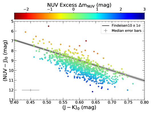
Figure 1: NUV versus NIR color-color diagram for the 842 RGs with GALEX NUV magnitudes. From this, the NUV excess is calculated by subracting the measured (NUV-J)₀ magnitudes and the expected values given the fiducial relation from Findeisen & Hillenbrand (2010) and the measured (J-K)₀ colors. The targets are color-coded by their NUV excess values, with redder colors indicating stronger excess (more negative values). The grey symbol represents the median error bars.

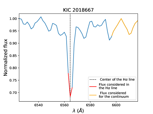
Figure 2: Example of LAMOST spectrum for KIC 2018667. The center of the H$\alpha$ line is indicated by the vertical dashed lines. The flux used to compute the H$\alpha$ index (Eq. 1) is represented in red for the H$\alpha$ line and in orange for the continuum.

2.2 Measuring the H$\alpha$ index

Using the H$\alpha$ line, we followed an approach similar to the one commonly used to measure the S-index (Gomes da Silva et al. 2021), which steps are described in Sect. 2.2 of Gehan et al. (2022). We used LAMOST Data Release 7, which is the same we used in Gehan et al. (2022) to measure the S-index. We computed the H$\alpha$ index as (Cincunegui et al. 2007)

$$S_{\mathrm{H\alpha}}=\frac{F_{\mathrm{H\alpha}}}{F_{\mathrm{C}}},$$ (1)

where $F_{\mathrm{H\alpha}}$ is the integrated flux in the H$\alpha$ line centered at 6562.801 Å  (in red in Fig. 2) using a triangular bandpass with a full width at half maximum of 1.5 Å, and $F_{\mathrm{C}}$ is the continuum level (in orange in Fig. 2) obtained by integrating the flux comprised in a square bandpass centered on 6605 Å  with a width of 20 Å. We validated our $S_{\mathrm{H\alpha}}$ measurements only for spectra presenting a high enough signal-to-noise ratio, in a similar way as in Sect. 2.2 of Gehan et al. (2022). Uncertainties were also computed in a similar way as in Sect. 2.2 of Gehan et al. (2022). When several spectra were available for a given star, we computed the H$\alpha$-index as the median of all the H$\alpha$-indices measured for each individual spectrum.

We note that our method defines the center of the H$\alpha$ line as the wavelength associated with the local flux minimum, which can be slightly offset compared to the actual center of the H$\alpha$ line. This is illustrated by Fig. 2, where the red wavelength range is not symmetrical with respect to our identified line center. However, we checked that our procedure does not impact significantly the inferred $S_{\mathrm{H\alpha}}$ values (see Appendix B).

We were able to measure the H$\alpha$ index for 3362 RGs, which is a slightly larger number than the 3130 RGs for which we obtained a S-index measurement using the same LAMOST spectra (Gehan et al. 2022). This is expected since for late-type stars, the signal-to-noise ratio is higher in the vicinity of the H$\alpha$ line than in the vicinity of the CaII lines used to measure the S-index. We report our measurements in Table 2. Our sample includes 185 binaries, among which there are 24 close binaries identified by Gaulme et al. (2020), 9 close binaries identified by Benbakoura et al. (2021), as well as 22 close binaries and 130 wide binaries identified by Gaia DR3 (Gaia Collaboration et al. 2023a).

Table 2: NUV excess and H$\alpha$ index measured for the Gaulme et al. (2020) sample.

KIC	NUV excess (mag)	Uncertainty (mag)	H$\alpha$ index	Uncertainty
6836321	0.054	0.368	0.411	0.015
6925082	1.292	0.383	0.404	0.007
6925158	1.061	0.406	0.387	0.000
7006979	0.591	0.366	0.376	0.001
7090906	1.154	0.438	0.392	0.001
7093179	0.243	0.423	0.397	0.005
7094142	1.781	0.377	0.402	0.001
7103297	1.064	0.407	0.390	0.001
7178170	0.475	0.415	0.380	0.001
7186274	0.765	0.409	0.385	0.003
…	…	…	…	…

3 Near-ultraviolet excess and H$\alpha$ index of red giants

In this section and the ones that follow, we adopted the measurements of the photometric index $S_{\mathrm{ph}}$, the oscillation frequency at maximum amplitude $\nu_{\mathrm{max}}$, the height of the Gaussian envelope employed to model the oscillation excess power $H_{\mathrm{max}}$, and the rotation period $P_{\mathrm{rot}}$ that were obtained by Gaulme et al. (2020). The chromospheric S-index $S_{\mathrm{CaII}}$ was adopted from Gehan et al. (2022).

3.1 Relation between activity indicators

In the following we compare the $\Delta m_{\mathrm{NUV}}$ and the $S_{\mathrm{H\alpha}}$ activity indicators with the $S_{\mathrm{CaII}}$ and $S_{\mathrm{ph}}$ activity indices for our RG sample. These are shown in Figure 3, where our sample is split into different subsets, namely single spotless stars (in grey), single spotted stars (in blue), binary spotted stars (in black) and spotted stars with ambiguous binary versus single status (in green). We discuss Fig. 3 in the following subsections.

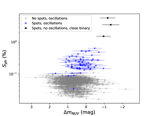
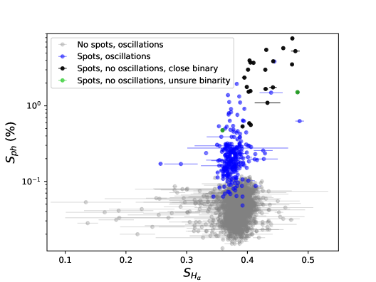
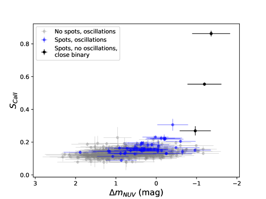
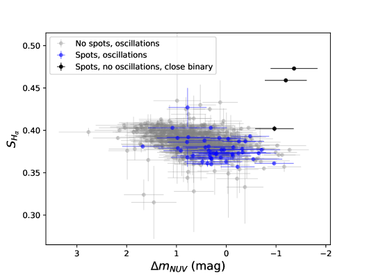
Figure 3: Relation between different activity indicators. Gray dots refer to regular photometrically inactive RGs (i.e. with no evidence of spot modulation) that display oscillations. Blue dots refer to photometrically active RGs (i.e. exhibiting spot modulation) with partially suppressed oscillations. Black dots refer to photometrically active and non-oscillating RGs in close binary systems, which were identified by Gaulme et al. (2020). Green dots refer to non-oscillating RGs with ambiguous binary versus single status; we do not have NUV excess data for these stars. $S_{\mathrm{ph}}$ is the photometric modulation as measured by Gaulme et al. (2020) (in log scale), which is an indicator of photospheric activity. $S_{\mathrm{CaII}}$ is the S-index as measured by Gehan et al. (2022), which is an indicator of chromospheric activity. The H$\alpha$ index $S_{\mathrm{H\alpha}}$ and the NUV excess $\Delta m_{\mathrm{NUV}}$ are the chromospheric activity indicators measured in the current study using LAMOST and GALEX data, respectively.

3.1.1 Relation with the photometric index $S_{\mathrm{ph}}$

We observe a correlation between $\Delta m_{\mathrm{NUV}}$ and $S_{\mathrm{ph}}$ for the photometrically active RGs with evidence of spots, associated to a Pearson correlation coefficient of $r=0.259$ (p-value of 0.046). Gehan et al. (2022) also observed a correlation between $S_{\mathrm{ph}}$ and chromospheric activity measured by $S_{\mathrm{CaII}}$ for active RGs. However, we do not observe any significant correlation or anti-correlation between $\Delta m_{\mathrm{NUV}}$ and $S_{\mathrm{ph}}$ for the inactive spotless RGs, for which we measure $r=-0.023$ (p-value of 0.532). In contrast, Gehan et al. (2022) found an anti-correlation between $S_{\mathrm{ph}}$ and chromospheric activity measured by $S_{\mathrm{CaII}}$ for the inactive RGs. To the extent of our knowledge, the relation between $\Delta m_{\mathrm{NUV}}$ and $S_{\mathrm{ph}}$ has never been checked before, even for main-sequence stars.

Similarly, we also observe a correlation between $S_{\mathrm{ph}}$ and $S_{\mathrm{H\alpha}}$. This is consistent with the findings of Newton et al. (2017) and García Soto et al. (2023) for M dwarfs, who observed a positive correlation between photometric variability amplitude and the H$\alpha$ emission line strength. However, the positive correlation that we observe emerges only when including the active single and binary RGs, for which we measure $r=0.291$ (p-value of $1.8\times 10^{-6}$). When considering only the inactive RGs, we do not observe any significant correlation or anti-correlation since we obtain $r=0.028$ (p-value of 0.122). To the extent of our knowledge, it is the first time that the relation between the the H$\alpha$ emission line strength and $S_{\mathrm{ph}}$ is explored for RGs.

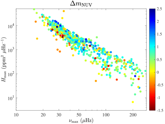
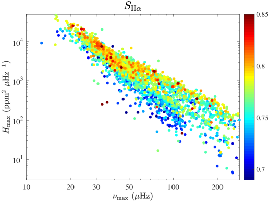
Figure 4: Activity level (colorscale) as a function of oscillations frequency at maximum amplitude $\nu_{\mathrm{max}}$ ($x$-axis) and height of the Gaussian envelope employed to model the oscillation excess power $H_{\mathrm{max}}$ ($y$-axis). The values of $\nu_{\mathrm{max}}$ and $H_{\mathrm{max}}$ come from Gaulme et al. (2020). Left: $\Delta m_{\mathrm{NUV}}$ colorscaled. Right: $S_{\mathrm{H\alpha}}$ colorscaled.

3.1.2 Relation with the S-index $S_{\mathrm{CaII}}$

We observe a correlation between the NUV excess and the S-index, associated to $r=0.383$ (p-value of $2.1\times 10^{-22}$). Since the S-index is a proxy of the strength of surface magnetic fields (Babcock 1961; Petit et al. 2008; Aurière et al. 2015; Brown et al. 2022), our result indicates that the NUV excess is indeed a proxy for the strength of surface magnetic fields. This is consistent with Findeisen et al. (2011) who observed a correlation between the NUV excess and chromospheric activity from the H and K lines of CaII for G-dwarfs. We note that the three RGs that are in close binaries (KIC 7869590, KIC 10908111, KIC 11554998) present values of the NUV excess that are the largest, i.e. the more negative. To the extent of our knowledge, it is the first time that the relation between the NUV excess and $S_{\mathrm{CaII}}$ is explored for RGs.

In addition, we observe an anticorrelation between the S-index and the H$\alpha$ index for inactive RGs, for which we measure $r=-0.128$ (p-value of $1.0\times 10^{-11}$). For active RGs, we do not observe any significant correlation or anti-correlation since we obtain $r=-0.038$ (p-value of 0.550). In the case of RGs in close binaries, the S-index and the H$\alpha$ index seem to be positively correlated. The correlation between the flux in the H$\alpha$ and the CaII lines is still not fully understood (Gomes da Silva et al. 2022). In the case of the Sun, the flux in the H$\alpha$ and the $S_{\mathrm{CaII}}$ lines is known to be correlated with the presence of active regions, and tightly follows the solar magnetic cycle (Livingston et al. 2007). However, the picture is much less straightforward for other stars, where the correlation between the flux in the H$\alpha$ and the $S_{\mathrm{CaII}}$ lines presents a large dispersion (Cincunegui et al. 2007; Walkowicz & Hawley 2009; Gomes da Silva et al. 2011, 2014; Meunier et al. 2022). The correlation appears to be strongly positive for stars with high activity levels, while all types of correlations tend to be observed in the low-activity regime, ranging from negative to positive correlations, including correlations close to 0. Since the cores of the CaII and H$\alpha$ lines are formed at different temperatures, hence at different heights in the chromosphere (Mauas & Falchi 1994, 1996; Mauas et al. 1997; Fontenla et al. 2016), we can then expect these two lines to trace different activity phenomena (Cincunegui et al. 2007; Meunier & Delfosse 2009; Gomes da Silva et al. 2022). The different sensitivity of these lines to spots, plages, or filaments could explain the various correlations observed for different stars (Meunier & Delfosse 2009). In particular, Meunier & Delfosse (2009) stated that the contribution of emission in plages in CaII and H$\alpha$ should lead to a correlation very close to 1 between the flux in these two lines. However, the presence of dark filaments at the surface, mostly visible in H$\alpha$, introduces flux absorption that should decrease the correlation. Moreover, many filaments do not coincide exactly with active regions, which further contributes in decreasing the correlation between the flux in the CaII and H$\alpha$ lines. On the other hand, filaments well correlated with plages would lead to an anticorrelation.

Gomes da Silva et al. (2022) also noticed that the correlation between the CaII and H$\alpha$ indices depends on the balance between the flux in the line core and in the line wings of H$\alpha$. They found that using a smaller bandpass with a width of 0.6 Å  maximises the correlation between the flux in the CaII and H$\alpha$ lines. Their result suggests that the H$\alpha$ line core is positively correlated with the S-index, while the H$\alpha$ wings are generally anti-correlated with the line core. We found that the differences in S_Hα are mild when using a bandpass width of 0.6 Å  instead of 1.5 Åand do not impact our results (see Appendix C).

3.1.3 Relation between the NUV excess and the H$\alpha$ index

We observe an anticorrelation between the NUV excess and the H$\alpha$ index associated to $r=-0.286$ (p-value of $2.7\times 10^{-11}$). To the extent of our knowledge, this is the first time that the relationship between the NUV excess and the H$\alpha$ index is explored. For a sample of nearby M-dwarfs, Stelzer et al. (2013) found a positive correlation between NUV and X-ray fluxes, as well as between H$\alpha$ and X-ray fluxes, but did not check the relation between NUV and H$\alpha$ fluxes. Since the NUV excess is a proxy of the chromospheric activity level, and the H$\alpha$ line is expected to trace activity at a lower height, with an important contribution from filaments, it is not necessarily surprising to observe an anticorrelation between $\Delta m_{\mathrm{NUV}}$ and $S_{\mathrm{H\alpha}}$, in the same way that we observed an anticorrelation between the S-index and $S_{\mathrm{H\alpha}}$ for active RGs (Sect. 3.1.2).

3.2 Relation with oscillation amplitude

Magnetic fields tend to inhibit convection, resulting in the partial or total suppression of oscillations (Gaulme et al. 2014, 2016; Beck et al. 2018; Benbakoura et al. 2021). Stars with low-amplitude oscillations or without oscillations are often associated with high S-index values (Bonanno et al. 2014; Gehan et al. 2022) and/or high $S_{\mathrm{ph}}$ values (García et al. 2010; Chaplin et al. 2011; Gaulme et al. 2014; Mathur et al. 2019; Gaulme et al. 2020; Benbakoura et al. 2021). We consistently find here that the RGs exhibiting low-amplitude oscillations also tend to present large (i.e. negative) $\Delta m_{\mathrm{NUV}}$ values (left panel of Fig. 4).

On the other hand, we observe that the H$\alpha$ index is correlated with the oscillations amplitude (right panel of Fig. 4). This striking trend is opposite to what we obtain with $\Delta m_{\mathrm{NUV}}$ (left panel of Fig. 4), $S_{\mathrm{ph}}$ (Gaulme et al. 2020) and $S_{\mathrm{CaII}}$ (Gehan et al. 2022). However, this is not necessarily surprising given that our sample is composed of a majority of spotless RGs, for which we found that $S_{\mathrm{H\alpha}}$ is not significantly correlated with $S_{\mathrm{ph}}$, while being anti-correlated with the $S_{\mathrm{CaII}}$ and $\Delta m_{\mathrm{NUV}}$. As we discussed in Sect. 3.1.2, this different behaviour for $S_{\mathrm{H\alpha}}$ could come from the larger sensitivity of the H$\alpha$ line to filaments (Meunier & Delfosse 2009). In the case of the Sun, the number and length of filaments follow the sunspot cycle (Mazumder et al. 2021), implying that higher activity levels for the Sun results in an increased number and length of filaments. If the same is true for RGs, higher activity levels could result in an increase of the filaments contribution to $S_{\mathrm{H\alpha}}$, hence in a decrease in $S_{\mathrm{H\alpha}}$. To the extent of our knowledge, this is the first time that the relation between the oscillation amplitude and the chromospheric activity indicators $S_{\mathrm{H\alpha}}$ and $\Delta m_{\mathrm{NUV}}$ is checked.

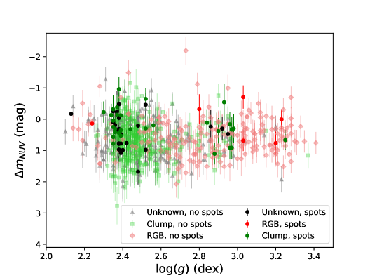
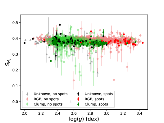
Figure 5: Activity level as a function of the surface gravity $\log g$ (left:$\Delta m_{\mathrm{NUV}}$, right: $S_{\mathrm{H\alpha}}$). The color indicates the evolution stage: red symbols refer to RGB stars; green symbols refer to RC stars; and gray symbols refer to stars with an unknown evolution stage. Stars with spot modulation are represented by darker dots than stars with no spot modulation. The symbol changes as a function of evolution stage for stars with no spot modulation.

3.3 Relation with $\log g$

We do not observe any correlation between $\Delta m_{\mathrm{NUV}}$ and $\log g$ (left panel of Fig. 5), as we obtain $r=0.077$ (p-value of 0.271) and $r=0.031$ (p-value of 0.527) for red giant branch (RGB, shell-hydrogen burning) and red clump (RC, core-helium burning) stars, respectively. On the contrary, Gehan et al. (2022) found a correlation between $\log g$ and chromospheric activity as measured by the S-index. Since the number of RGs with $\Delta m_{\mathrm{NUV}}$ measurements is much smaller than the number of RGs with S-index measurements obtained by Gehan et al. (2022), it is not surprising that we do not observe a correlation between $\Delta m_{\mathrm{NUV}}$ and $\log g$. Indeed, Gehan et al. (2022) also noticed the absence of significant correlation between the level of chromospheric activity from spectroscopy and $\log g$ for the RGs analyzed by Gomes da Silva et al. (2021), due to the rather small number of RGs in their sample.

On the other hand, we observe a slight anti-correlation between $S_{\mathrm{H\alpha}}$ and $\log g$ (right panel of Fig. 5) associated to $r=-0.108$ (p-value of $1.7\times 10^{-3}$) and $r=-0.158$ (p-value of $8.3\times 10^{-11}$) for RGB and RC stars, respectively. This trend reminds what Gehan et al. (2022) obtained for the photometric index $S_{\mathrm{ph}}$. Indeed, Gehan et al. (2022) observed that $S_{\mathrm{ph}}$ decreases with $\log g$ in the case of inactive RGs for which, in the absence of detectable photometric modulation, $S_{\mathrm{ph}}$ is just the standard deviation of the light curve, which is dominated by surface granulation and inversely proportional to $\log g$ (e.g., Bastien et al. 2013, 2016). As we observe here with $S_{\mathrm{H\alpha}}$, Gehan et al. (2022) reported a stronger anti-correlation – steeper slope – between $S_{\mathrm{ph}}$ and $\log g$ for RC than RGB stars. This trend was already visible in Bastien et al. (2016), based on the flicker index that traces the granulation amplitude in a similar way than $S_{\mathrm{ph}}$ for inactive stars. Stellar mass $M$, more than the different evolutionary stage between RGB and clump stars, seems to explain this trend. Indeed, we can see in Fig. 4 of Bastien et al. (2016) that more massive clump stars, i.e. secondary clump stars, have $\log g\gtrsim 2.6$. We can see in Fig. 5 (left panel) of Gehan et al. (2022) that the different trend observed for RC stars compared to RGB stars is mainly due to such RC stars with $\log g\gtrsim 2.6$, hence to secondary clump stars, which are more massive than RGB stars. This is confirmed by Corsaro et al. (2017), who found that the granulation amplitude decreases with $M$ (see their Fig. 7, upper panel). Moreover, previous works for oscillating RGs have also noticed that the maximum mode amplitude, which is proportional to the granulation amplitude, decreases with $M$, for both RGB and clump stars (Huber et al. 2010, 2011; Mosser et al. 2011, 2012; Stello et al. 2011; Kallinger et al. 2014; Vrard et al. 2018). Such a trend can be explained by the dependence of the depth of the external convective envelope with $M$. At a given $\log g$, the depth of the convective envelope is mainly determined by the effective temperature $T_{\mathrm{eff}}$, with deeper convective envelopes associated to lower $T_{\mathrm{eff}}$ (Pinsonneault et al. 2001; van Saders & Pinsonneault 2012). Since $T_{\mathrm{eff}}$ and $M$ are correlated at a given $\log g$ for both RGB and RC stars, this implies that lower-mass RGs have deeper convective envelopes, which can in turn result in higher granulation amplitudes, hence to higher oscillations amplitudes.

4 Close binarity: impact of tidal interactions versus fast rotation on the NUV excess and the H$\alpha$ index

It has been observed that for a given rotation period, RGs in binary systems undergoing spin-orbit resonance or tidal locking exhibit larger $S_{\mathrm{ph}}$ (Gaulme et al. 2020) and larger $S_{\mathrm{CaII}}$ (Gehan et al. 2022) than single RGs or RGs in binary systems with no special tidal configuration. Here, we check the impact of fast rotation and tidal interactions on $\Delta m_{\mathrm{NUV}}$ and $S_{\mathrm{H\alpha}}$.

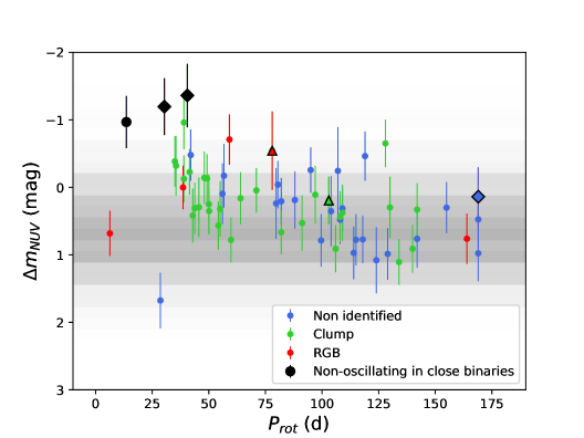
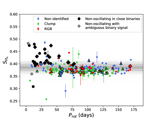
Figure 6: Activity level as a function of the rotation period $P_{\mathrm{rot}}$. The RGB and RC stars are represented in red and green, respectively, while RGs with an unidentified evolutionary stage are in blue. Black symbols correspond to non-oscillating RGs in close binaries from Gehan et al. (2022). Triangles and diamonds represent wide ($P_{\mathrm{orb}}$ ¿ 150 d) and close ($P_{\mathrm{orb}}\leq$ 150 d) binaries identified by Gaia DR3, respectively. The gray background indicates the distribution of the activity level for inactive stars, where a darker shade corresponds to a larger number of stars. Left: $\Delta m_{\mathrm{NUV}}$ as a function of $P_{\mathrm{rot}}$. Right: $S_{\mathrm{H\alpha}}$ as a function of $P_{\mathrm{rot}}$.

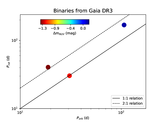
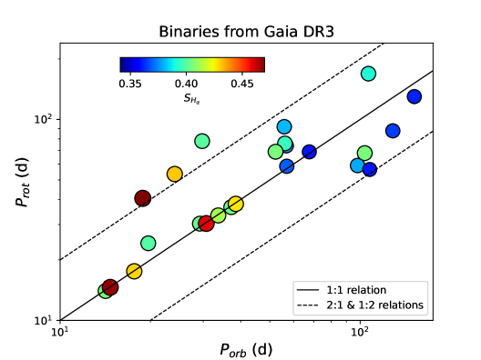
Figure 7: Rotation period as a function of the orbital period for the close binaries listed by Gaia DR3. The continuous lines represent the 1:1 relation, while the dashed lines represent the 2:1 and 1:2 relations. Left: The symbols’ colors indicate the value of $\Delta m_{\mathrm{NUV}}$. Left: The symbols’ colors indicate the value of $S_{\mathrm{H\alpha}}$.

4.1 Impact of surface rotation

Gaulme et al. (2020) reported rotation periods of 370 RGs from measurements of spot modulation. We measure $\Delta m_{\mathrm{NUV}}$ for 63, and $S_{\mathrm{H\alpha}}$ for 283 of them. By including all the types of active RGs – binaries and single stars – we observe an anti-correlation between the NUV excess and the rotation period (Fig. 6, left panel), associated to a Pearson correlation coefficient of $r=-0.185$ (p-value of $6.8\times 10^{-8}$). This is consistent with the findings of Dixon et al. (2020) for RGs and Godoy-Rivera et al. (2021) for subgiants, as both works found that the NUV excess increases (i.e., becomes more negative) for faster rotators. Such a decrease of magnetic activity as a function of the rotational period had already been observed using the S-index (Noyes et al. 1984; Aurière et al. 2015). We note that Gehan et al. (2022) did not observe such a clear trend between the S-index and the rotation period, but noticed that it probably originates from the small range of spectral types covered in their study. Overall, our findings provide further evidence for the rotation-activity connection in post main-sequence stars (Lehtinen et al. 2020).

We note that the three RGs with the largest $\Delta m_{\mathrm{NUV}}$ in the left panel of Fig. 6 are among the fastest rotators in our sample. However, these three non-oscillating RGs also belong to close binaries, suggesting that fast rotation alone does not explain the observed large $\Delta m_{\mathrm{NUV}}$ and that tidal interactions are actually responsible for it. We note that one single RG, KIC 11521644, stands among the fastest rotators in our sample while displaying the smallest $\Delta m_{\mathrm{NUV}}$ among the RGs with measured rotation period (blue symbol on the bottom left in the left panel of Fig. 6). However, KIC 11521644 is actually likely a contaminant since we notice the presence of another close bright source on the Target Pixel File of its Kepler light curve. In addition, we observed that its surface modulation is detectable only from the KEPSEISMIC light curve but not on the simple aperture photometry (SAP) light curve. Since KEPSEISMIC light curves are built on enlarged photometric apertures with respect to the SAP, it tends to confirm it is an artifact.

We also observe that RGs in close binaries present in average larger $S_{\mathrm{H\alpha}}$ values than single RGs (right panel of Fig. 6) , for a given rotation period. This is similar to what we observe for the NUV excess (left panel of Fig. 6), the photometric index (Gaulme et al. 2014, 2020; Benbakoura et al. 2021) and the S-index (Gehan et al. 2022), reinforcing that the faster rotation induced by tidal interactions is not enough to explain the enhanced magnetic activity observed for RGs in close binaries. Furthermore, $S_{\mathrm{H\alpha}}$ seems to decrease as a function of the rotation period (right panel of Fig 6) period, but this anti-correlation is unclear if we consider only the single RGs and discard the stars in close binaries. Newton et al. (2017) observed a negative correlation between the H$\alpha$ emission line strength and the rotation period, but they worked on a larger sample (466 stars) of less evolved stars (dwarfs), having a different spectral type than the RGs in our sample (M-type stars while our sample includes G- and K-type stars). A plausible explanation for this difference is that M dwarfs tend to be very active (e.g. Kiraga & Stepien 2007), which could increase the contribution of the chromospheric emission in the core of the H$\alpha$ line compared to the contribution of filaments in the wings of the H$\alpha$ line.

4.2 Impact of tidal interactions

To investigate the role of tidal interactions in the level of NUV emission, Fig. 7 displays the rotational versus orbital periods of the RGs in close binaries in our sample (similarly as Gaulme et al. (2014) and Benbakoura et al. (2021) for $S_{\mathrm{ph}}$, as well as Gehan et al. (2022) for the S-index). We found no GALEX data for the close binaries studied by Gaulme et al. (2014); Benbakoura et al. (2021) and we are left with only three RGs in close binaries with available rotation period from Gaulme et al. (2020) and orbital period from Gaia DR3. Two fast rotators exhibit large $\Delta m_{\mathrm{NUV}}$ values, namely KIC 7869590 and KIC 11554998, while one slow rotator exhibits a small $\Delta m_{\mathrm{NUV}}$, namely KIC 7661609. Notably, we observe in the left panel of Fig. 7 that the two fast-rotating RGs belong respectively to a tidally locked system (1:1 resonance, KIC 11554998) and to a system in spin-orbit resonance (rotation period being twice the orbital period, KIC 7869590), while the system with the slowly-rotating RG does not have any special tidal configuration. In a similar fashion (right panel of Fig. 7), we also observe that RGs in systems that are tidally locked or in spin-orbit resonance display the largest values of $S_{\mathrm{H\alpha}}$ compared to the systems that do not have any special tidal configuration.

Previous studies already noticed a possible relation between NUV emission and binarity for more evolved stars on the asymptotic giant branch (stars undergoing both shell-hydrogen and shell-helium burning, Sahai et al. 2008, 2011; Ortiz & Guerrero 2016; Montez et al. 2017). For less evolved stars on the RGB and the RC, Dixon et al. (2020) observed that their binary sample presents larger $\Delta m_{\mathrm{NUV}}$ values, stating however that this is likely due to fast rotation since the RGs in binaries are found to be rapidly rotating more often than single RGs. To the extent of our knowledge, the link between large $\Delta m_{\mathrm{NUV}}$ values and tidal interactions was never established before. In addition, Montes et al. (1995) reported excess H$\alpha$ emission for 51 chromospherically active binaries, including both RS Cvn and BY Dra systems. They observed for these systems a slight decrease of the excess H$\alpha$ emission with the rotation period, as well as a good correlation with the CaII K line.

Enhanced magnetic activity for RGs in systems that are either tidally locked or undergoing spin-orbit resonance has been previously observed using $S_{\mathrm{ph}}$ (Gaulme et al. 2014; Benbakoura et al. 2021) and $S_{\mathrm{CaII}}$ (Gehan et al. 2022) as activity indicators. Our results show that such systems also exhibit enhanced NUV excess and H$\alpha$ index, reinforcing the findings of Gehan et al. (2022) that tidal interactions in close binaries drive abnormally large magnetic fields in RGs, rather than fast rotation by itself. Investigating the physical mechanism(s) at work is beyond the scope of this work (but see e.g. Beck et al. 2023).

5 Classification of active red giants

We here provide criteria to classify the active RGs, that have rotation period measurements resulting from the presence of spots on their photosphere producing photometric rotational modulation. Those criteria come from the findings of Gaulme et al. (2020), Gehan et al. (2022), Oláh et al. (2021) and the present study and are summarized in Fig. 8.

5.1 Fast-rotating red giants

We focus here on fast-rotating RGs ($P_{\mathrm{rot}}<50$ d). Gaulme et al. (2020) found that RGs belonging to a close binary system (red category in Fig. 8) displays $S_{\mathrm{ph}}$ values about one order of magnitude larger than that of single RGs (blue category in Fig. 8). This result suggested two possibilities: either tidal interactions somehow lead to stronger magnetic fields, or the spot distribution differs between binary and single red giants, leading to a different photometric variability. Gehan et al. (2022) could conclude that tidal interactions indeed lead to stronger magnetic fields, by also finding significantly larger chromospheric $S_{\mathrm{CaII}}$ values for close binary compared to single RGs. In the present study, we also find that RGs in close binaries tend to exhibit larger chromospheric $S_{\mathrm{H\alpha}}$ and $\Delta m_{\mathrm{NUV}}$ values than single RGs, reinforcing the conclusions of Gehan et al. (2022). In addition, Oláh et al. (2021) found that a large fraction of the 61 flaring RGs they studied are likely to belong to close binary systems. Hence, the presence of flares is a possible additional indication of close binarity for RGs.

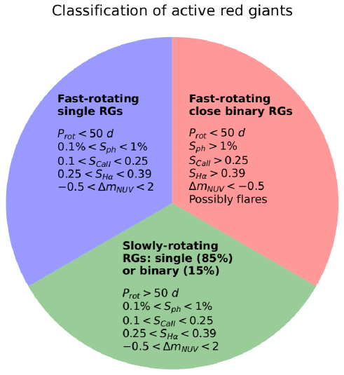
Figure 8: Diagram classifying the active red giants, i.e. exhibiting rotational modulation due to the presence of spots, based on the findings of Gaulme et al. (2020, $P_{\mathrm{rot}}$ and $S_{\mathrm{ph}}$), Gehan et al. (2022, $S_{\mathrm{CaII}}$), Oláh et al. (2021, presence of flares for RGs in close binaries) and the present study ($S_{\mathrm{H\alpha}}$ and $\Delta m_{\mathrm{NUV}}$).

5.2 Slower rotating red giants

Slower rotating RGs ($P_{\mathrm{rot}}\geq 50$ d, green category in Fig. 8) tend to exhibit similar activity levels ($S_{\mathrm{ph}}$, $S_{\mathrm{CaII}}$, $S_{\mathrm{H\alpha}}$, $\Delta m_{\mathrm{NUV}}$, low flare occurrence) than single fast-rotating RGs, whether they are in a binary or single configuration. Based on Gaulme et al. (2020), slower rotating RGs have a 85% probability of being single, and a 15% probability of being part of a binary system.

6 Conclusions

Stellar activity indicators are crucial probes of the relation between stellar rotation and magnetic fields. In this paper, we measured two indicators of chromospheric magnetic activity for RGB and RC stars, namely the NUV excess above the photospheric level for 842 stars using data from the GALEX survey, as well as the H$\alpha$ index for 3362 stars measured using spectroscopic data from the LAMOST survey. Other activity indicators have been previously measured for this stellar sample, namely the photometric index tracing the level of photospheric activity, $S_{\mathrm{ph}}$, measured from Kepler light curves (Gaulme et al. 2020), and the S-index tracing the level of chromospheric activity, $S_{\mathrm{CaII}}$, measured from LAMOST spectroscopic data (Gehan et al. 2022). We first investigated the relation between these activity indices, with the main findings being:

• for active RGs exhibiting spots, we found a positive correlation between the NUV excess and $S_{\mathrm{ph}}$, as well as between the H$\alpha$ index and $S_{\mathrm{ph}}$. For inactive RGs, we observed on the contrary an absence of significant correlation. To the extent of our knowledge, this the first time that the relationship between the NUV excess and $S_{\mathrm{ph}}$ is checked;

• we found a positive correlation between the NUV excess and the S-index, indicating that the NUV excess is proportional to the strength of surface magnetic fields. This is consistent with the findings of Findeisen et al. (2011) for G dwarfs. To the extent of our knowledge, this the first time that the relationship between the NUV excess and the S-index is explored. However, we observe a different relation between the H$\alpha$ index and the S-index $S_{\mathrm{CaII}}$, with no significant correlation for active RGs exhibiting spots detected from the Kepler light curves, and an anti-correlation for inactive RGs without spots. This reflects the fact that the relation between the flux in the H$\alpha$ and the CaII lines is still not fully understood (Gomes da Silva et al. 2022), partly due to the larger sensitivity of the H$\alpha$ line to the presence of dark filaments at the surface than the other activity indicators studied here (Meunier & Delfosse 2009);

• we found an anti-correlation between the NUV excess and the H$\alpha$ index. This is possibly due to both activity proxies probing different chromospheric heights. To the extent of our knowledge, this the first time that the relationship between the NUV excess and the H$\alpha$ index is explored.

Moreover, we noticed that the chromospheric NUV excess does not appear correlated with surface gravity, contrarily to the chromospheric S-index, although this may be explained by the smaller size of the sample with NUV excess measurements compared to the original sample with $S_{\mathrm{CaII}}$ measurements by Gehan et al. (2022). We also observe an anti-correlation between the H$\alpha$ index and surface gravity, which is hard to consistently explain given the complex relation between the H$\alpha$ and the level of chromospheric activity.

In addition, we found that stars with low-amplitude oscillations tend to exhibit larger NUV excess values, which is fully consistent with the expected suppression of oscillations in the presence of a magnetic field. We however observe that RGs with low-amplitude oscillations do not exhibit particularly large values of the H$\alpha$ index. To the extent of our knowledge, this is the first time that the relation between the oscillation amplitude and these two activity indicators is investigated.

Moreover, we obtain an anti-correlation between the NUV excess and the surface rotation period, consistently with previous studies (Dixon et al. 2020; Godoy-Rivera et al. 2021). We observe a similar correlation between the H$\alpha$ index and the rotation period, although only when including the targets in close-binaries.

Finally, we investigated the impact of tidal interactions on the NUV excess and the H$\alpha$ index based on RGs in our sample that belongs to close binary systems, identified by Gaulme et al. (2020) and Gaia DR3 (Gaia Collaboration et al. 2023a). Our sample includes 7 close binaries for which we measured the NUV excess as well as 55 close binaries for which we measured the H$\alpha$ index. We observed that for similar rotation periods, RGs in close binaries tend to exhibit larger NUV excess and H$\alpha$ index values than single RGs, similarly to what Gaulme et al. (2020) observed with $S_{\mathrm{ph}}$ and to what Gehan et al. (2022) observed with the S-index. In addition, we found that RGs in close binaries that are in a configuration of spin-orbit resonance or tidally-locked exhibit larger NUV excess and H$\alpha$ index values than the RGs in binary systems that do not have any special tidal configuration. This result reinforces the finding of Gehan et al. (2022) that RGs in systems undergoing spin-orbit resonance exhibit larger magnetic fields, which are not only due to the faster rotation rate induced by tidal interactions. Investigating the physical mechanism(s) leading to an enhanced magnetic activity for RGs in close binaries is left to future work.

Based on the findings of Gaulme et al. (2020), Gehan et al. (2022), Oláh et al. (2021) and the present study, we provided criteria to classify the active RGs, based on their rotation periods, photometric ($S_{\mathrm{ph}}$) and chromospheric ($S_{\mathrm{CaII}}$, $S_{\mathrm{H\alpha}}$, $\Delta m_{\mathrm{NUV}}$) activity indices, as well as the presence or absence of flares. Since $\sim$90 millions stars have ultraviolet photometric observations from GALEX, and $\sim$ 10 million stars have LAMOST spectra, where the signal-to-noise ratio is higher in the vicinity of the H$\alpha$ line than the CaII H & K lines, NUV excess and H$\alpha$ index measurements could help identifying tidally-interacting systems in future works, in addition to the photometric index (Gaulme et al. 2020), the S-index (Gehan et al. 2022) and the presence of flares (Oláh et al. 2021).

Appendix A Details of the NUV excess

A.1 Note on the photometric systems

We note that the GALEX magnitudes are reported in the AB system, and the 2MASS magnitudes are reported in the Vega system. While the GALEX magnitudes may be converted into the Vega system following the transformations of Bianchi et al. (2017, see their Equations 2 and 3), this is not needed when calculating the NUV excess. This is inherited from the definition of the NUV excess by Findeisen & Hillenbrand (2010), who derived the fiducial relation combining the native GALEX and 2MASS photometric systems (see their Figure 4). Regardless of the above, as the shift from one photometric system to the other is just an additive constant, the activity-rank of our targets would remain identical in either of them.

A.2 Impact of metallicity on the NUV excess

Near the submission of this work, Lu et al. (2023) posted a method for obtaining photometric metallicities based on GALEX NUV data. Motivated by this, we tested the influence of metallicity on the NUV excess as follows. As the Lu et al. 2023 catalog was not yet published, we searched for metallicity information for our sample by crossmatching with the catalog of Andrae et al. (2023), which reported stellar parameters (T${}_{\text{eff}}$, $\log{g}$, and [M/H]) derived from the Gaia DR3 BP/RP spectra. Using these [M/H] values, we found our targets to span a range of metallicties centered around a slightly sub-solar value (median [M/H] = -0.07 dex), in agreement with the rest of the Kepler field, (e.g., Godoy-Rivera et al. submitted). Indeed, we noted a correlation between the NUV excess and the [M/H] values, which implies that at least part of the NUV activity can be attributed to metallicity (see also Olmedo et al. 2019). Nevertheless, we tested removing this effect via linear regression, and found that the majority of the NUV-active targets remain as such after accounting for this metallicity-dependence. Thus, the reported NUV excess values are robust against the effect of metallicity.

Appendix B Impact of fitting a Gaussian to the H$\alpha$ line on the H$\alpha$ index

Our method defines the center of the H$\alpha$ line as the wavelength associated with the local flux minimum. A more conservative way consists in fitting a Gaussian to the H$\alpha$ line in the vicinity of the local minimum, and to define the center of the H$\alpha$ line as the center of the Gaussian. For 850 RGs randomly selected in our sample, we found the H$\alpha$ line center by fitting a Gaussian on a wavelength range of width 3 Å  centered on the wavelength associated with the local flux minimum. We then compared the $S_{\mathrm{H\alpha}}$ values obtained with and without a Gaussian fit and found that the differences are mild, associated to a relative deviation below 3% in more than 98% of the cases (Fig. 9). Our approach presents the advantage of not requiring any fit to the H$\alpha$ line, hence being faster and avoiding potential fit convergence issues.

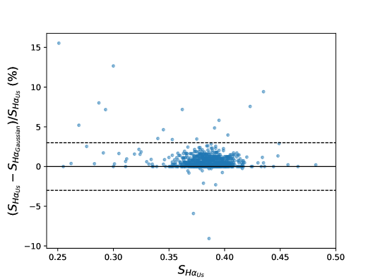
Figure 9: Relative deviation between our $S_{\mathrm{H\alpha}}$ values and $S_{\mathrm{H\alpha}}$ computed by identifying the center of the H$\alpha$ line through a Gaussian fit. The continuous line indicates a null relative deviation, while the dashed lines indicate relative deviations of $\pm$ 3 %.

Appendix C Impact of the width of the triangular bandpass on the H$\alpha$ index

Gomes da Silva et al. (2022) found that using a smaller triangular bandpass for the H$\alpha$ core line with a width of 0.6 Å  instead of 1.5 Å  maximises the correlation between the flux in the CaII and H$\alpha$ lines. Hence, we checked how using a bandpass width of 0.6 Å  instead of 1.5 Å  impacts our results (see Sect. 2.2) and found that the differences in S_Hα are mild. Indeed the relative deviation between $S_{\mathrm{H\alpha}}$ measured with these two bandpass widths is below 3% in more than 95% of the cases (Fig. 10). Hence, using a bandpass width of 0.6 Å  or 1.5 Å  does not change significantly the trends we obtain. A plausible explanation is that the much lower spectral resolution of LAMOST compared to the High Accuracy Radial velocity Planet Searcher (HARPS), which spectra are used by Gomes da Silva et al. (2022), results in fewer data points in a given bandpass, mitigating the impact of the H$\alpha$ wings on the H$\alpha$ index. Nevertheless, LAMOST presents the advantage of having observed a larger number of stars than high-resolution spectrographs like HARPS.

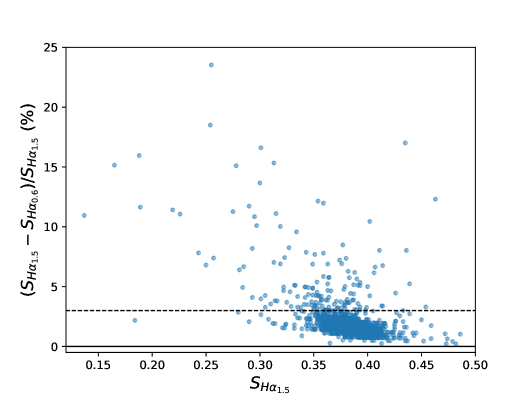
Figure 10: Relative deviation between $S_{\mathrm{H\alpha_{\mathrm{1.5}}}}$ and $S_{\mathrm{H\alpha_{\mathrm{0.6}}}}$, computed using a triangular bandpass for the core line with a width of 1.5 Å  and 0.6 Å, respectively, as a function of $S_{\mathrm{H\alpha_{\mathrm{1.5}}}}$ that we use in this study. The continuous line indicates a null relative deviation, while the dashed lines indicate a relative deviation of 3 %.