Vertex Fitting In Low-Material Budget Pixel Detectors

Abstract

This paper provides a detailed description of a vertex fitting algorithm suitable for precision measurements in low-energy particle physics experiments. An accurate reconstruction of low-momentum trajectories can be accomplished by reducing the material budget of the detector to a few per mill of the radiation length. This limits the multiple scattering undertaken by particles inside the detector and improves the vertex fitting accuracy. However, for sufficiently light detection systems, additional sources of errors, such as the intrinsic spatial resolution of the sensors, must be considered in the reconstruction of the vertex parameters. The algorithm developed in this work provides a complete treatment of multiple scattering and spatial resolution in the context of vertex fitting for light pixel detectors. In addition to this, a study of the vertex reconstruction in the low-material budget pixel detector of the Mu3e experiment is presented.

I Introduction

With the increase of the instantaneous and integrated beam luminosities, the requirements of particle physics experiments for precise tracking and vertexing detectors, with high radiation tolerance, have become more stringent e.g., SNOEYS2023168678 ; Hartmut2018 ; CARNESECCHI2019608 ; MOSER201685 . In this regard, silicon pixel sensors can provide high granularity, low material budget structures and the radiation-hardness that most experiments need, e.g., MOSER201685 ; SPANNAGEL2019612 ; Abelev_2014 ; ARNDT2021165679 . It is important, however, that precise detection systems are developed in conjunction with equally performing analysis methods for the reconstruction of particle trajectories and decay vertices, e.g. FRUHWIRTH1987444 ; BILLOIR1992139 ; Waltenberger2007 ; RevModPhys.82.1419 . To this aim, several fitting algorithms have been designed and optimized over the years to deal with hit selection, pattern recognition, errors calculations and high track multiplicity (see for instance Mankel_2004 ; RevModPhys.82.1419 and references therein). The practical implementation of these methods must be tailored around the actual detector and magnetic field configuration of the experiments. This makes tracking and vertexing a topic which is in continuous evolution adapting itself to the new challenges set by upcoming experiments.

This study addresses the problem of vertex fitting in the low-material budget pixel detector of the Mu3e experiment ARNDT2021165679 . As explained in section II, the detector design has been optimized to minimize Multiple Coulomb Scattering (MS) effects on particle trajectories and signal kinematics. However, for light detectors such as Mu3e, the intrinsic pixel resolution becomes another limiting factor in the vertex reconstruction which cannot be ignored. Under these circumstances, the vertex fitting should account for MS and pixel resolution in the error calculations as well as for any energy loss in the detector which may hamper tracks momentum reconstruction. The present algorithm deals with all these sources of errors and it is illustrated in section III whilst in section IV, a comparative study is made among different inclusive scenarios that encompass: (A) MS only; (B) MS and pixel resolution together; (C) all sources of errors (MS, pixel resolution and energy losses) are included.

II The low-material budget Mu3e pixel detector

The Mu3e experiment aims to find or exclude the rare Charged Lepton Flavour (CLF) violating muon decay:

$$\mu^{+}\rightarrow e^{+}e^{-}e^{+}$$ (1)

at Branching Ratios (BR) $>10^{-16}$ ARNDT2021165679 . This threshold is $4$ orders of magnitude smaller than previous experimental upper limits ($10^{-12}$) BELLGARDT19881 and $38$ orders of magnitude larger than theoretical Standard Model (SM) calculations (BR $=10^{-54}$), e.g., MARCIANO1977303 ; RevModPhys.73.151 . However, new theoretical models predict the existence of extra degrees of freedom beyond the SM which may bring CLF violation within the reach of near future experiments such as Mu3e, e.g., KAKIZAKI2003210 ; DEGOUVEA201375 . Consequentially, an observation of $\mu^{+}\rightarrow e^{+}e^{-}e^{+}$ at single event sensitivities aimed by the Mu3e experiment will imply scenarios of new physics.

The process in (1) yields a relatively simple decay topology with the 3 final state leptons produced at the same vertex of interaction and momentum vectors, $\vec{p}$, determined by the energy and momentum conservation for decaying muons at rest. The main background processes in Mu3e measurements are the muon internal conversion $\mu^{+}\rightarrow e^{+}e^{-}e^{+}+\nu_{e}+\bar{\nu}_{\mu}$ (BR $\approx 10^{-5}$) and the combination of one electron and 2 positrons from independent sources, e.g., one Bhabha electron plus two Michel positrons $\mu^{+}\rightarrow 2\times(e^{+}+\nu_{e}+\bar{\nu}_{\mu})+e^{-}$ BELLGARDT19881 .

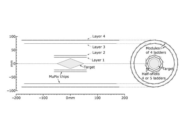
Figure 1: Scheme of the central barrel of the Mu3e pixel detector, side and x-y views ARNDT2021165679 .

The aimed single event sensitivity of $2\cdot 10^{-15}$, during phase I of the experiment, can be achieved with an energy-momentum resolution of $\lesssim 1$ MeV/c and by using precise vertexing and timing systems ARNDT2021165679 .

The energy spectrum of the decay particles in the Mu3e experiment extends up to $m_{\mu}/2$, where $m_{\mu}$ is the muon mass. In this low-energy region, MS poses a serious challenge to the reconstruction of particle trajectories and signal kinematics. To minimize MS, Mu3e uses a low-material budget pixel detector ($0.1\%$ of the radiation length, X_o, per layer). This is made of high-voltage monolithic active pixel sensors PERIC2007876 that can be thinned down to $50\text{\,}\mathrm{\SIUnitSymbolMicro m}$ or $0.05\%$X_o. The rest of the material budget of the detector is used in the flex-tape that provides mechanical support and the electrical routing to the sensors.

Figure 1 shows the schematic of the foreseen Mu3e tracker central station which is important for vertex fitting and track reconstruction ARNDT2021165679 . Two recurl stations, one up-stream and one down-stream, will also be part of the final detector design. These increase the angular acceptance of the experiment and allow to measure long-armed trajectories to achieve improved momentum resolution.

The layers have cylindrical symmetry and are concentrically placed around the target, a hollow double cone made of Mylar 100 mm in length and with a base radius of 19 mm. The target is placed in a solenoid magnetic field of 1 T with the base at a minimum distance of $\approx 4$ mm from the innermost layer of the pixel tracker. Particle trajectories bend inwards following helical trajectories around the field lines possibly making multiple re-curls. Each layer of the pixel detector is sectioned in sub-elements called ladders. A ladder is a series of chips mounted on the same flex-tape. There are 8, 10, 24 and 28 ladders for layer 1, 2, 3 and 4, respectively. For instance, the innermost layer of the tracker, crucial for vertex fitting, is made of 8 ladders each one tilted by a 45^∘ angle with respect to the neighbours. This configuration forms a 8-sided surface which extends for $\sim 12$ cm or 6 chips length, see figure 1.

The intrinsic detector spatial resolution is set by the pixel sensitive area, $80\times 80$$\text{\,}\mathrm{\SIUnitSymbolMicro m}$². Pixel resolution becomes more important for high-momentum trajectories for which MS is lower. However, for low-material budget detectors such as Mu3e, this effect cannot be ignored at any momentum and it must be treated simultaneously with MS.

III Vertex fitting in the Mu3e detector

Vertex reconstruction can be accomplished in two steps: vertex finding and vertex fitting, see e.g., RevModPhys.82.1419 . The former consists in grouping trajectories that have been most likely produced in the same decay process. The latter involves finding the most likely vertex coordinates $(x,y,z)_{\text{v}}$ and the initial momentum vectors of all clustered tracks. In Mu3e, vertex finding is accomplished by considering all possible combinations of two positive and one negative tracks in the detector within time frames of 64 ns. For the vertex fitting, a least-squares optimization algorithm has been developed based on the method illustrated in BILLOIR1992139 .

III.1 Track parameters and uncertainties

Trajectories are defined by 6 parameters ($[x,y],z,\phi,\lambda,k)$. These are the coordinates of one point along the track, the angles $\phi$ and $\lambda$ defining the direction of the tangent vector to the trajectory and the factor $k=(p/q)^{-1}$ where $q$ is the charge of the particle and $p$ is the magnitude of the momentum vector. The following relationships among the momentum components in the global Cartesian frame and the angles $\phi$ and $\lambda$ hold true:

$$\left\{\begin{aligned} p_{x}&=p\,\text{cos}(\lambda)\,\text{cos}(\phi)\,,\\ p_{y}&=p\,\text{cos}(\lambda)\,\text{sin}(\phi)\,,\\ p_{z}&=p\,\text{sin}(\lambda)\,,\\ R_{\perp}&=\frac{p\,\text{cos}(\lambda)}{q\,B}\,,\\ \phi&\in[0,2\pi]\,,\\ \lambda&\in[-\pi/2,\pi/2]\,,\end{aligned}\right.$$ (2)

where $B=B_{z}$ is the homogeneous magnetic field directed along the beam-line $\hat{z}$ and $R_{\perp}$ is the transverse radius of the trajectory.

The input measurements to fit are the values of the track parameters at a given Reference Surface (RS) along with their covariance matrix ($\Xi$): ($[x,y],z,\phi,\lambda,k,\Xi)_{\text{meas}}$. In this study, the RS is the innermost layer of the pixel detector which is the closest one to the expected real vertex position. The coordinates $x,y$ are not independent and can be given in a single expression by using a local reference frame with center in the middle of the pixel area $(\bar{x},\bar{y},\bar{z})$ and base vectors $(\hat{u},\hat{z^{\prime}})$. The vector $\hat{z^{\prime}}$ is parallel to the global coordinate $\hat{z}$ while $\hat{u}$ is perpendicular to it and parallel to the pixel surface, see figure 2. The equations that link the local coordinates to the global ones are:

$$\begin{array}[]{lll}u=\left(x-\bar{x}\right)\text{cos}(\gamma)+\left(y-\bar{y}\right)\text{sin}(\gamma)\,,\\ z^{\prime}=z-\bar{z}\,,\\ \phi^{\prime}=\phi\,,\\ \lambda^{\prime}=\lambda\\ k^{\prime}=k\end{array}$$ (3)

where the angle $\gamma$ is the orientation of the pixel with respect to the $x$ axis of the global reference frame. Following the equations in 3, the track parameters at the RS become $(u,z,\phi,\lambda,k)$ .

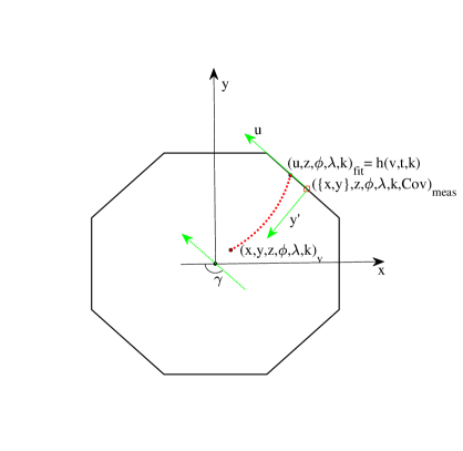
Figure 2: Sketch of the RS in the Mu3e vertex fitting. The axes of the global (local) reference frame are drawn in black (green); the $\hat{z^{\prime}}$ axis perpendicular to the $x-y$ plane is not shown. The parameters (${x,y},z)_{\text{meas}}$ are placed in the geometrical centre of the pixel surface $\square$. The fit parameters ($u,z,\phi,\lambda,k)_{\text{fit}}$ are obtained by forward propagating vertex parameters ($x,y,z,\phi,\lambda,k)_{\text{v}}$ via a function $h=h(\textbf{v}=(x,y,z)_{\text{v}},\textbf{t}(\phi_{\text{v}},\lambda_{\text{v}}),k_{\text{v}}))$.

The covariance matrix can be written as the sum of two terms, i.e., $\Xi_{\text{meas}}=\Xi_{\text{track}}+\Xi_{\text{phys}}$. The term $\Xi_{\text{track}}$ accounts for the uncertainties accumulated during track fitting while $\Xi_{\text{phys}}$ accounts for MS and pixel resolution at the RS. Pixel resolution contributes to the smearing of the hit position by $\sigma_{l}=l/\sqrt{12}$, where $l$ is the length of the pixel side. The MS changes the direction of the track upon crossing the RS. The tilt can be approximated by a Gaussian distribution with zero mean and standard deviation $\theta_{\text{MS}}$ Yao_2006 :

$$\theta_{\text{MS}}=13.6\,\left[\text{MeV/c}\right]\,\frac{q}{p}\sqrt{\frac{x}{\beta^{2}\text{X}_{o}}}\left(1+0.038\,\text{ln}\left(\frac{d}{\text{X}_{o}}\right)\right)\,.$$ (4)

In the previous equation $\beta$ is the relativistic velocity and $d$ is the distance travelled by the particle in the RS. From eq. 4, the changes in $\phi$ and $\lambda$ due to MS, $\sigma_{\phi}$ and $\sigma_{\lambda}$, can be obtained by projecting $\theta_{\text{MS}}$ onto the transverse and longitudinal planes, respectively, see e.g., VALENTAN2009728 :

$$\sigma_{\lambda}=\theta_{\text{MS}}\,,\\$$ (5)

and

$$\sigma_{\phi}=\theta_{\text{MS}}/\text{cos}(\lambda)\,.$$ (6)

In addition to MS and pixel resolution, an error $\sigma_{k}$ on the track curvature (or $k$) is introduced in $\Xi_{\text{meas}}$ to account for the energy lost by electrons and positrons in the detector, see e.g., Mankel_2004 . Although energy losses in a thin silicon layer like the RS are negligible RevModPhys.60.663 , they are nevertheless included in the present vertex fitting algorithm to provide a complete treatment of the errors. Without loss of generality, the covariance matrix in this study is written as $\Xi_{\text{meas}}$ = diag$\left\{\sigma_{u}^{2},\sigma_{z}^{2},\sigma_{\phi}^{2},\sigma_{\lambda}^{2},\sigma_{k}^{2}\right\}$ with $\sigma_{u}=\sigma_{z}=\sigma_{l}$.

III.2 Least-squares algorithm

In the vertex fitting, a map that links the track vertex parameters ($x,y,z,\phi^{i},\lambda^{i},k^{i})_{\text{v}}$ to the parameters at the RS ($u^{i},z^{i},\phi^{i},\lambda^{i},k^{i})_{\text{fit}}$ is needed, as shown in figure 2. In what follows, $i=1,2,3$ for the ($e^{-},e^{+},e^{+}$) in a Mu3e decay. Starting from the analytical expression of a helical trajectory of a charged particle in a magnetic field, this map can be written as: $h_{j}=h(\textbf{v},\textbf{t}^{i},k^{i}_{\text{v}})_{j}$, where $h_{j}=(u,z,\phi,\lambda,k)_{\text{fit}}$ for $j=1,2,...,5$, $\textbf{v}=(x,y,z)_{\text{v}}$ and $\textbf{t}=(\phi,\lambda)_{\text{v}}$, see section VII for the analytic expressions of $h_{j}$. In first approximation, this function can be linearized near some initial guessed vertex parameters ($\textbf{v}_{o},\textbf{t}_{o},k_{o}$):

$$h(\textbf{v}_{o}+\delta\textbf{v},\textbf{t}_{i,o}+\delta\textbf{t}_{i},k_{i,o}+\delta k_{i})_{j}\simeq h(\textbf{v}_{o},\textbf{t}_{i,o},k_{i,o})_{j}+D_{i}\,\delta\textbf{v}+E_{i}\,\delta\textbf{t}_{i}\,+F_{i}\,\delta k_{i},$$ (7)

where, for each track $i$, the matrices $D_{i}$, $E_{i}$ and $F_{i}$ have dimensions $5\times 3$, $5\times 2$ and $5\times 1$, respectively, and are calculated as follows:

$$\begin{array}[]{lll}D^{j}_{n}=\frac{\partial h_{j}}{\partial\textbf{v}_{n}}\hskip 14.22636pt\textbf{v}_{n}=x_{\text{v}},y_{\text{v}},z_{\text{v}}\,\hskip 14.22636pt\text{for }n=1,2,3,\\ E^{j}_{m}=\frac{\partial h_{j}}{\partial\textbf{t}_{m}}\hskip 14.22636pt\textbf{t}_{m}=\phi_{\text{v}},\lambda_{\text{v}}\,\hskip 14.22636pt\text{for }m=1,2,\\ F^{j}=\frac{\partial h_{j}}{\partial k_{\text{v}}}\end{array}$$ (11)

From the definitions in eq. 7, a quadratic cost function, $\chi^{2}$, is defined:

$$\chi^{2}=\sum_{i}\left(\delta q_{i}-D_{i}\delta\textbf{v}-E_{i}\delta\textbf{t}_{i}-F_{i}\delta k_{i}\right)^{T}W_{i}\left(\delta q_{i}-D_{i}\delta\textbf{v}-E_{i}\delta\textbf{t}_{i}-F_{i}\delta k_{i}\right).$$ (12)

where $W=\Xi^{-1}$ is the weight matrix (see for instance BILLOIR1985115 ) and $\delta q$ is the residual at the RS:

$$\delta q^{i} =(u^{i},z^{i},\phi^{i},\lambda^{i},k^{i})_{\text{meas}}-h(\textbf{v}_{o},\textbf{t}^{i}_{o},k_{o}^{i})\,.$$ (13)

Equation 12 is the total normalized error, due to the approximation in eq. 7, expressed as a function of $\delta\textbf{v}$, $\delta\textbf{t}$ and $\delta k$. The accuracy of such an approximation can be seen in figure 3(a) where the RMS of the deviations $(x,y,z)_{\text{meas}}-(x,y,z)_{\text{fit}}$ at the RS are plotted versus fit iteration number.

The corrections to the initial guessed vertex parameters can be found by minimizing the cost function, i.e., by solving the following system of equations:

$$\left\{\begin{aligned} &\sum_{i}A_{i}^{T}\delta\textbf{v}+\sum_{i}B^{T}_{i}\delta\textbf{t}_{i}+\sum_{i}H^{T}_{i}\delta k_{i}=\sum_{i}T_{i},\\ &B_{i}\delta\textbf{v}+C_{i}\delta\textbf{t}_{i}+G_{i}\delta k_{i}=U_{i},\\ &H_{i}\delta\textbf{v}+G_{i}^{T}\delta\textbf{t}_{i}+L_{i}\delta k_{i}=Z_{i}.\end{aligned}\right.$$ (14)

where

$$A_{i}^{T}=D_{i}^{T}W_{i}D_{i}\,,\hskip 14.22636ptB_{i}=E_{i}^{T}W_{i}D_{i}\,\hskip 14.22636ptC_{i}=E_{i}^{T}W_{i}E_{i}\,,$$ (15)

$$G_{i}=E_{i}^{T}W_{i}F_{i}\,,\hskip 14.22636ptH_{i}=F^{T}W_{i}D_{i}\,,\hskip 14.22636ptL_{i}=F_{i}^{T}W_{i}F_{i}\,,$$

$$T_{i}=D_{i}^{T}W_{i}\delta q_{i}\,,\hskip 14.22636ptU_{i}=E_{i}^{T}W_{i}\delta q_{i}\,\hskip 14.22636ptZ_{i}=F_{i}^{T}W_{i}\delta q_{i}.$$

The solutions of system described in eq. 14 are:

$$\delta\textbf{v} =\left[\left(\sum_{i}A^{T}-\sum_{i}B^{T}_{i}C^{-1}_{i}B_{i}\right)+\left(\sum_{i}B^{T}_{i}C^{-1}_{i}G_{i}-\sum H_{i}^{T}\right)N_{1}N_{3}\right]^{-1}$$ (16)

$$\times\left(\sum_{i}T_{i}-\sum_{i}B_{i}^{T}C^{-1}_{i}U_{i}+\left(\sum_{i}B^{T}_{i}C^{-1}_{i}G_{i}-\sum H_{i}^{T}\right)N_{1}N_{2}\right),$$

$$\delta k_{i} =N_{1}\left(N_{2}-N_{3}\delta\textbf{v}\right),$$

$$\delta\textbf{t}_{i} =C_{i}^{-1}\left(U_{i}-B_{i}\delta\textbf{v}-G_{i}\delta k_{i}\right),$$

where:

$$N_{1} =\left(L_{i}-G^{T}_{i}C^{-1}_{i}G_{i}\right)^{-1}\,,$$ (17)

$$N_{2} =\left(Z_{i}-G^{T}_{i}C^{-1}_{i}U_{i}\right)\,$$

$$N_{3} =\left(H_{i}-G^{T}_{i}C^{-1}_{i}B_{i}\right)\,.$$

From eq. 16 the covariance matrices for the track parameters at the vertex can be calculated:

$$\text{Cov}(\textbf{v}) =\left[\left(\sum_{i}A^{T}-\sum_{i}B^{T}_{i}C^{-1}_{i}B_{i}\right)+\left(\sum_{i}B^{T}_{i}C^{-1}_{i}G_{i}-\sum H_{i}^{T}\right)N_{1}N_{3}\right]^{-1},$$ (18)

$$\text{Cov}(k_{i}) =L_{i}^{-1}+\left(N_{1}N_{3}\right)\text{Cov}(\textbf{v})\,\left(N_{1}N_{3}\right)^{T},$$

$$\text{Cov}(\textbf{t}_{i}) =C_{i}^{-1}+\left(C_{i}^{-1}B_{i}\right)\text{Cov}(\textbf{v})\left(C_{i}^{-1}B_{i}\right)^{T}+\left(C_{i}^{-1}G_{i}\right)\text{Cov}(k)\left(C_{i}^{-1}G_{i}\right)^{T}.$$

III.3 Algorithm testing

Geant4 based Monte-Carlo (MC) simulations of Mu3e decays have been carried out for testing the vertex fitting described in section III.2. The procedure followed by the test was:

1. Hit parameters at the RS, $(u_{i},z_{i},\phi_{i},\lambda_{i},k_{i})_{MC}$, were obtained from MC trajectories.

2. $(u_{i},z_{i})_{MC}$ were smeared by using pixel resolution, i.e., by adding a random offset derived from a uniform distribution with mean and standard deviation $(0,\sigma_{l})$. The $(\phi_{i},\lambda_{i})$ angles were tilted according to the errors in equations 5 and 6 for values of the MS pooled from a Gaussian distribution with $\hat{\mu}=0$ and $\sigma=\theta_{\text{MS}}$. The error on $k_{i}$ was obtained by drawing from a Gaussian distribution with mean zero and a standard deviation $\sigma_{k}$.

3. From point 1 and 2, $\Xi_{\text{meas}}$ was derived together with the weight matrix $W$.

4. The initial parameters $\textbf{v}_{o}=x_{o},y_{o},z_{o}$ were obtained as the average coordinates of the tracks intersection points. Since two tracks can have up to two intersections, the one that is met first when back propagating the track parameters from the RS to the target is retained in the calculation of the average value. If two tracks do not intersect, the point of closest approach is used. The vectors $\textbf{t}_{o}$ were extracted at the point of closest approach of the trajectories to $\textbf{v}_{o}$ whilst $k_{o}$ was directly obtained from the track reconstruction carried out before the vertex fitting.

5. From equations 7 and 11, the residuals at the RS were calculated and thus the corrections $\delta\textbf{v}$, $\delta k_{i}$ and $\delta\textbf{t}_{i}$ in eq. 16. Only a few iterations were required to minimize the $\chi^{2}$ in eq. 12, as it can be seen in figure 3(b).

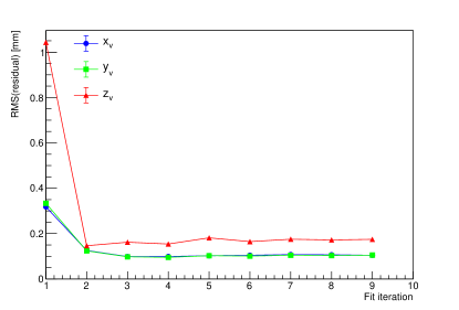
(a)

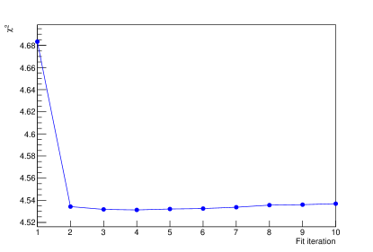
(b)

Figure 3: Typical RMS of the residuals $(x,y,z)_{meas}-(x,y,z)_{fit}$ at the RS (a) and the $\chi^{2}$ minimization (b) as a function of the fit iteration number.

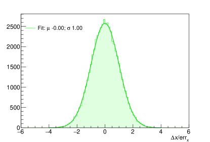
(a)

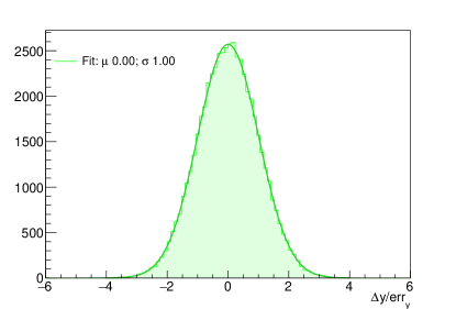
(b)

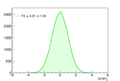
(c)

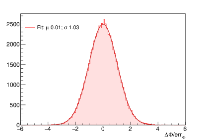
(d)

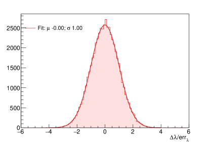
(e)

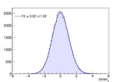
(f)

Figure 4: Pull distributions (a-f) of the track parameters at the vertex: ($x,y,z,\phi,\lambda,k)_{\text{v}}$ for test trajectories obtained by following the steps described in the text.

A precise determination of the fit errors depends on the correct characterization of $\Xi_{\text{meas}}$ and its propagation, e.g., WOLIN1993493 Lund_2009 . In the present study, the covariance matrix of the vertex parameters was calculated by propagating $\Xi_{\text{meas}}$ from the RS to the vertex point by using equations 18. A key test of the algorithm developed in this section consists in plotting the pull distributions of the track parameters. The pull of a variable $X$ with expected value $\mu_{X}$ and standard error $\sigma_{X}$ is:

$$P=\frac{\left(X-\mu_{X}\right)}{\sigma_{X}}.$$ (19)

If the error and the residual in eq. 19 are well characterized, the pulls are normally distributed.

Figure 4 shows the normal distributions for the pulls of all the track parameters at the vertex $(x,y,z,\phi,\lambda,k)_{\text{v}}$ as calculated by the present vertex fitting algorithm.

IV Comaprative study of error sources

In section III.1, the explicit form of the covariance matrix was given by including the contribution of MS, pixel resolution and energy losses at RS: $\Xi_{\text{meas}}=\text{diag}\left\{\sigma_{u}^{2},\sigma_{z}^{2},\sigma_{\phi}^{2},\sigma_{\lambda}^{2},\sigma_{k}^{2}\right\}$. In this section, the relative weights of these errors on the determinations of the fit vertex parameters and their uncertainties are discussed. Three different inclusive scenarios have been considered: (A) MS only; (B) MS and pixel resolution are both included; (C) all sources of errors (MS, pixel resolution and energy losses) are considered. These three scenarios are summarized in table 1.

It must be noted that the kernel of $\Xi_{\text{meas}}$ grows larger going from scenario (A) to (C) along with the dimensionality of the problem, see for example (BILLOIR1992139, ). For instance, if the energy loss and pixel resolution at the RS are ignored, MS remains the only source of uncertainty against which all measurements are fixed but $(\phi_{i},\lambda_{i})_{\text{meas}}$, i.e., $\Xi_{\text{meas}}=\text{diag}\left\{\sigma_{\phi}^{2},\sigma_{\lambda}^{2}\right\}$. These 6 angles can be fitted with 3 vertex variables $(x,y,z)_{\text{v}}$ thus simplifying eq. 16, see e.g., schenk2013vertex .

Table 1: Scenrarios A,B,C in the comparative study of the vertex fitting.

Scenario	$\Xi_{\text{meas}}$	measurements	fit parameters	errors
A	$\text{diag}\left\{\sigma_{\phi}^{2},\sigma_{\lambda}^{2}\right\}$	$(\phi,\lambda)_{\text{meas}}$	$(x,y,z)_{\text{v}}$	MS
B	$\text{diag}\left\{\sigma_{u}^{2},\sigma_{z}^{2},\sigma_{\phi}^{2},\sigma_{\lambda}^{2}\right\}$	$(u,z,\phi,\lambda)_{\text{meas}}$	$(x,y,z,\phi,\lambda)_{\text{v}}$	MS, pixel
C	$\text{diag}\left\{\sigma_{u}^{2},\sigma_{z}^{2},\sigma_{\phi}^{2},\sigma_{\lambda}^{2},\sigma_{k}^{2}\right\}$	$(u,z,\phi,\lambda,k)_{\text{meas}}$	$(x,y,z,\phi,\lambda,k)_{\text{v}}$	MS, pixel, $\Delta E$

Panels (a-e) in figure 5 show the the deviations between MC vertex parameters of simulated Mu3e decays and those obtained from vertex fitting in scenarios (A) and (B), respectively. From figure 5(a-c), it can be seen that the fit accuracy for the determinations of $(x,y,z)_{\text{v}}$ does not improve when the pixel resolution is included in covariance matrix. However, a significant improvement is found on the determinations of $(\phi_{i},\lambda_{i})_{\text{v}}$, as shown in figure 5(d,e). The results for scenario (C) are statistically the same as for scenario (B). The former being the only case in which the fit attempts to optimize the track parameter $k$, see table 1. As expected, having neglected the energy losses at the RS, track curvatures do not vary significantly throughout the vertex fitting, as it can be seen in figure 5(f).

The improved fit accuracy of case (C) with respect to scenario (A) for the coordinates of the momentum vector $p_{x}$, $p_{y}$ and $p_{z}$ is shown in figure 6(a-c). This improvement reflects also onto the determination of the average total momentum which is $\sim$10$\%$ smaller in scenario (C) than the corresponding average in scenario (A), and thus closer to real MC value (in the hypothesis of decaying muons at rest), see figure 6(d).

The invariant mass of simulated Mu3e decays, calculated from the fit vertex parameters in scenarios (A) and (C), is shown in figure 7. As expected, no significant difference is seen in the two fit scenarios. In fact, the magnitude of the invariant mass is dominated by the muon rest mass over which the fit accuracy has little leverage.

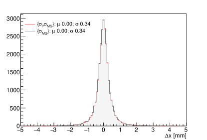
(a)

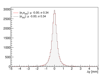
(b)

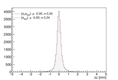
(c)

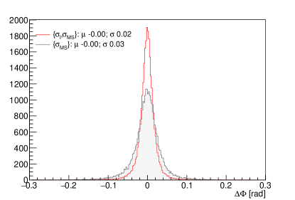
(d)

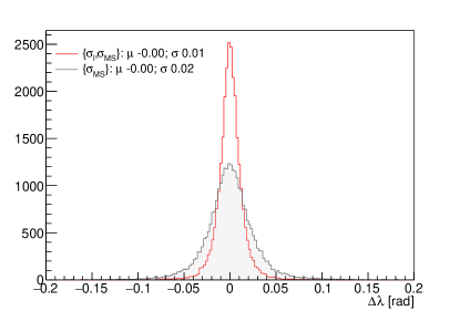
(e)

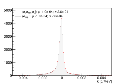
(f)

Figure 5: Deviations between the fit and MC track parameters at the vertex. The legends show the mean and standard deviation obtained from a Gaussian fit in scenarios (A) [full gray] and (B or C) [empty red], respectively.

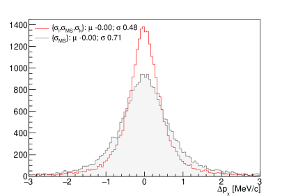
(a)

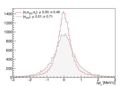
(b)

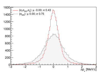
(c)

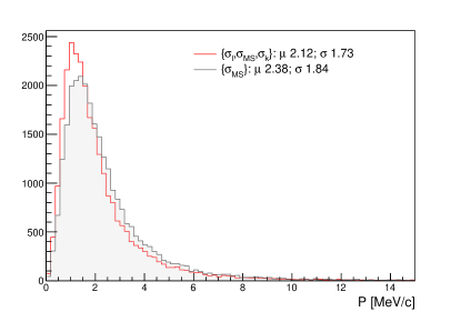
(d)

Figure 6: Deviations between the fit and MC momentum coordinates $p_{x}$, $p_{y}$ and $p_{z}$ panels (a-c) and total momenutm $P$ in panel (d) for scenario (A) [full gray] and (C) [empty red], respectively. In (a,b,c), the legends show the mean and standard deviation obtained from a Gaussian fit whilst the legend in (d) shows the average and stadard deviation of the distributions.

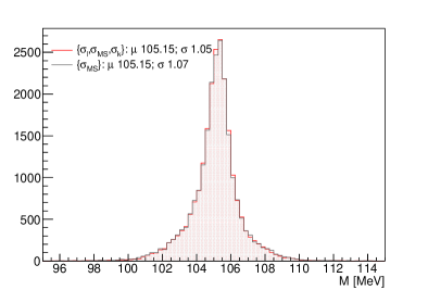
Figure 7: Rreconstructed invariant mass for vertices with $\chi^{2}<15$ and total momentum $P<4$ MeV/c, scenario (A) [full gray] and (C) [empty red], respectively.

V Conclusion

In this paper, a simple least-squares method has been described which can be applied to reconstruct decay vertices in experiments equipped with pixel detectors. The relative weights of 1) MS, 2) pixel resolution and 3) energy losses to the final reconstruction accuracy has been investigated in the case study of the Mu3e low-material budget pixel detector. The exhaustive errors treatment of the present study goes beyond the MS-only approximation showing a significant improvement of the fit accuracy when the intrinsic pixel resolution is accounted for. This should encourage a rigorous treatment of the pixel resolution in the development of future reconstruction algorithms concerning precise particle physics measurements at low-energy.

VI Acknowledgements

I am grateful to the STFC grant for supporting this work. I wish to thank the members of the Mu3e Software and Analysis group for providing the simulation and track reconstruction software behind this study. I also want to thank Joel Goldstein, Niklaus Berger and Gavin Hesketh for all the detailed and useful discussions about this work. I also thank Naik Paras and Andre Schoning for their careful reading and useful comments.

VII Appendix 1: forward propagation of track parameters

The map $h(\textbf{v},\textbf{t},k)$ propagates a trajectory from the vertex to the hit at the RS. In this section, its analytical expression is derived by starting from the propagation of a track in the transverse plane and then along the beam direction.

Propagation in the transverse plane

In this study, trajectories are helices with symmetry axis $\hat{z}$ and transverse radius $R_{\perp}$ which sign is given by the charge $q$ of the particle, see eq. 2. We write $R_{\perp}=R$ cos($\lambda$) such as:

$$R:=\left\{\begin{aligned} &+\frac{p}{|q|B}\hskip 8.5359pt\text{if q }>0\text{ c.c.w rotation}\,\\ &-\frac{p}{|q|B}\hskip 8.5359pt\text{if q }<0\text{ c.w rotation}\,.\end{aligned}\right.$$ (20)

In the x-y plane, a helix is a circumference with center in $(x_{c},y_{c})$ and radius $R_{\perp}$. It is not difficult to prove that:

$$x_{c}=x_{\text{v}}-R_{\perp}\text{sin}(\phi_{\text{v}})\,,$$ (21)

$$y_{c}=y_{\text{v}}+R_{\perp}\text{cos}(\phi_{\text{v}})\,,$$

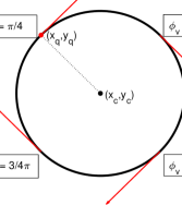
Figure 8: Sketch of a track with negative radius, as defined in eq. 20, projected on the x-y plane. The $\phi_{\text{v}}$ values are obtained by subtracting $\pi/2$ from the phase angle of the radial vector.

The transport equations in the transverse plane is obtained by calculating the coordinates $(x_{q},y_{q})$ of the intersection point between the track originating from $(x_{\text{v}},y_{\text{v}})$ and the detector ladder. In the x-y plane, the ladder profile is a line characterised by the parameters $y_{o}$ and $m$, see figure 9:

$$\left\{\begin{aligned} &(y_{q}-y_{c}(\textbf{v},\textbf{t},k))^{2}+(x_{q}-x_{c}(\textbf{v},\textbf{t},k))^{2}=R_{\perp}^{2}\,,\\ &y_{q}=m\,x_{q}+y_{o}\,,\\ &m=\text{tg}(\gamma)\,.\end{aligned}\right.$$ (22)

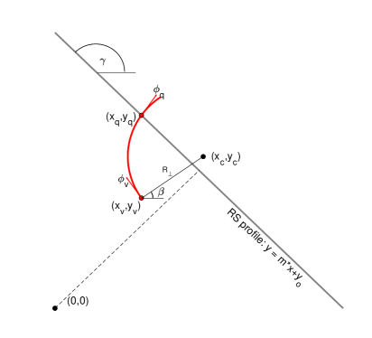
Figure 9: A sketch representing the intersection between a trajectory and the detector RS in the x-y plane.

In the previous equation, $\gamma$ is the angle of the detector ladder with respect to the global $\hat{x}$ axis. The parameter $y_{o}$ can be calculated by using $y_{\text{meas}}=tg(\gamma)x_{\text{meas}}+y_{o}$. In conclusion, the solutions of the system of equations 22 can be written as:

$$\begin{array}[]{l}x_{q}=\left(\begin{array}[]{c}-\frac{\mathrm{y_{o}}-\frac{\mathrm{y_{o}}+m\,\mathrm{x_{v}}+\sigma_{1}+m^{2}\,\mathrm{y_{v}}+\sigma_{2}-\sigma_{3}}{m^{2}+1}}{m}\\ -\frac{\mathrm{y_{o}}-\frac{\mathrm{y_{o}}+m\,\mathrm{x_{v}}-\sigma_{1}+m^{2}\,\mathrm{y_{v}}+\sigma_{2}-\sigma_{3}}{m^{2}+1}}{m}\end{array}\right)\\ \end{array}$$ (23)

and

$$y_{q}=\left(\begin{array}[]{c}\frac{\mathrm{y_{o}}+m\,\mathrm{x_{v}}+\sigma_{1}+m^{2}\,\mathrm{y_{v}}+\sigma_{2}-\sigma_{3}}{m^{2}+1}\\ \frac{\mathrm{y_{o}}+m\,\mathrm{x_{v}}-\sigma_{1}+m^{2}\,\mathrm{y_{v}}+\sigma_{2}-\sigma_{3}}{m^{2}+1}\end{array}\right)\,,\\ \mathrm{}\\$$ (24)

where

$$\begin{array}[]{l}\mathrm{}\\ \;\;\sigma_{1}=m\,\left[-R^{2}\,m^{2}\,{\mathrm{cos}\left(\mathrm{\lambda_{v}}\right)}^{2}\,{\mathrm{sin}\left(\mathrm{\phi_{v}}\right)}^{2}+R^{2}\,m^{2}\,{\mathrm{cos}\left(\mathrm{\lambda_{v}}\right)}^{2}\right.\\ \left.-2\,R^{2}\,m\,{\mathrm{cos}\left(\mathrm{\lambda_{v}}\right)}^{2}\,\mathrm{cos}\left(\mathrm{\phi_{v}}\right)\,\mathrm{sin}\left(\mathrm{\phi_{v}}\right)-R^{2}\,{\mathrm{cos}\left(\mathrm{\lambda_{v}}\right)}^{2}\,{\mathrm{cos}\left(\mathrm{\phi_{v}}\right)}^{2}\right.\\ \left.+R^{2}\,{\mathrm{cos}\left(\mathrm{\lambda_{v}}\right)}^{2}+2\,R\,m^{2}\,\mathrm{x_{v}}\,\mathrm{cos}\left(\mathrm{\lambda_{v}}\right)\,\mathrm{sin}\left(\mathrm{\phi_{v}}\right)+2\,R\,m\,\mathrm{x_{v}}\,\mathrm{cos}\left(\mathrm{\lambda_{v}}\right)\,\mathrm{cos}\left(\mathrm{\phi_{v}}\right)\right.\\ \left.+2\,R\,m\,\mathrm{y_{o}}\,\mathrm{cos}\left(\mathrm{\lambda_{v}}\right)\,\mathrm{sin}\left(\mathrm{\phi_{v}}\right)-2\,R\,m\,\mathrm{y_{v}}\,\mathrm{cos}\left(\mathrm{\lambda_{v}}\right)\,\mathrm{sin}\left(\mathrm{\phi_{v}}\right)\right.\\ \left.+2\,R\,\mathrm{y_{o}}\,\mathrm{cos}\left(\mathrm{\lambda_{v}}\right)\,\mathrm{cos}\left(\mathrm{\phi_{v}}\right)-2\,R\,\mathrm{y_{v}}\,\mathrm{cos}\left(\mathrm{\lambda_{v}}\right)\,\mathrm{cos}\left(\mathrm{\phi_{v}}\right)-m^{2}\,{\mathrm{x_{v}}}^{2}\right.\\ \left.-2\,m\,\mathrm{x_{v}}\,\mathrm{y_{o}}+2\,m\,\mathrm{x_{v}}\,\mathrm{y_{v}}-{\mathrm{y_{o}}}^{2}+2\,\mathrm{y_{o}}\,\mathrm{y_{v}}-{\mathrm{y_{v}}}^{2}\right]^{1/2}\\ \mathrm{}\\ \;\;\sigma_{2}=R\,m^{2}\,\mathrm{cos}\left(\mathrm{\lambda_{v}}\right)\,\mathrm{cos}\left(\mathrm{\phi_{v}}\right)\\ \mathrm{}\\ \;\;\sigma_{3}=R\,m\,\mathrm{cos}\left(\mathrm{\lambda_{v}}\right)\,\mathrm{sin}\left(\mathrm{\phi_{v}}\right)\,.\end{array}$$ (25)

A choice between the two solutions in equations 23 and 24 can be made by accounting for the track direction of motion and the vertex position relative to the hit.

For what is concerned with $\phi_{\text{v}}$, the following expression can be written, see figure 8:

$$\phi_{q}=\text{atan}\left(\frac{y_{q}-y_{c}(x_{\text{v}},y_{\text{v}},\phi_{\text{v}},\lambda_{\text{v}},k_{\text{v}})}{x_{q}-x_{c}(x_{\text{v}},y_{\text{v}},\phi_{\text{v}},\lambda_{\text{v}},k_{\text{v}})}\right)+\text{sign}(R)\pi/2\,.$$ (26)

Propagation along the beam axis

The propagation of helical trajectories along the $\hat{z}$ axis is characterized by the following equations VALENTAN2009728 :

$$\left\{\begin{aligned} &\lambda_{q}=\lambda_{\text{v}}\,,\\ &z_{q}=z_{\text{v}}+R_{\perp}\,\text{tan}(\lambda_{\text{v}})\left(\phi_{q}-\phi_{\text{v}}\right)\,.\end{aligned}\right.$$ (27)

References

References

- [1] W. Snoeys. Monolithic CMOS sensors for high energy physics — challenges and perspectives. NIM-A, 1056:168678, 2023.
- [2] H. F. W. Sadrozinski, A. Seiden, and N. Cartiglia. 4D tracking with ultra-fast silicon detectors. Rep. Prog. Phys., 81:026101, 2018.
- [3] F. Carnesecchi et al. Development of ultra fast silicon detector for 4D tracking. NIM-A, 936:608–611, 2019. Frontier Detectors for Frontier Physics: 14th Pisa Meeting on Advanced Detectors.
- [4] H. G. Moser. The Belle II DEPFET pixel detector. NIM-A, 831:85–87, 2016. Proceedings of the 10th International “Hiroshima” Symposium on the Development and Application of Semiconductor Tracking Detectors.
- [5] S. Spannagel. Technologies for future vertex and tracking detectors at CLIC. NIM-A, 936:612–615, 2019. Frontier Detectors for Frontier Physics: 14th Pisa Meeting on Advanced Detectors.
- [6] B. Abelev and The ALICE Collaboration. Technical design report for the upgrade of the ALICE inner tracking system. Journal of Physics G: Nuclear and Particle Physics, 41(8):087002, 2014.
- [7] K. Arndt et al. Technical design of the phase I Mu3e experiment. NIM-A, 1014:165679, 2021.
- [8] R. Frühwirth. Application of Kalman filtering to track and vertex fitting. NIM-A, 262(2):444–450, 1987.
- [9] P. Billoir and S. Qian. Fast vertex fitting with a local parametrization of tracks. NIM-A, 311(1):139–150, 1992.
- [10] W. Waltenberger, R. Frühwirth, and P. Vanlaer. Adaptive vertex fitting. Journal of Physics G: Nuclear and Particle Physics,, 34:N343, 2007.
- [11] A. Strandlie and R. Frühwirth. Track and vertex reconstruction: from classical to adaptive methods. Rev. Mod. Phys., 82:1419–1458, 2010.
- [12] R. Mankel. Pattern recognition and event reconstruction in particle physics experiments. Reports on Progress in Physics, 67(4):553, 2004.
- [13] U. Bellgardt et al. Search for the decay . Nuclear Physics B, 299(1):1–6, 1988.
- [14] W.J. Marciano and A.I. Sanda. Exotic decays of the muon and heavy leptons in gauge theories. Physics Letters B, 67(3):303–305, 1977.
- [15] Y. Kuno and O. Yasuhiro. Muon decay and physics beyond the standard model. Rev. Mod. Phys., 73:151–202, 2001.
- [16] M. Kakizaki, Y. Ogura, and F. Shima. Lepton flavor violation in the triplet Higgs model. Physics Letters B, 566(3):210–216, 2003.
- [17] A. de Gouvêa and P. Vogel. Lepton flavor and number conservation, and physics beyond the standard model. Progress in Particle and Nuclear Physics, 71:75–92, 2013. Fundamental Symmetries in the Era of the LHC.
- [18] I. Perić. A novel monolithic pixelated particle detector implemented in high-voltage CMOS technology. NIM-A, 582(3):876–885, 2007. VERTEX 2006.
- [19] W. M. Yao et al. Review of particle physics. Journal of Physics G: Nuclear and Particle Physics, 33(1):1, 2006.
- [20] M. Valentan, M. Regler, and R. Frühwirth. Generalization of the Gluckstern formulas II: multiple scattering and non-zero dip angles. NIM-A, 606(3):728–742, 2009.
- [21] H. Bichsel. Straggling in thin silicon detectors. Rev. Mod. Phys., 60:663–699, 1988.
- [22] P. Billoir, R. Frühwirth, and M. Regler. Track element merging strategy and vertex fitting in complex modular detectors. NIM-A, 241(1):115–131, 1985.
- [23] E. J. Wolin and L. L. Ho. Covariance matrices for track fitting with the Kalman filter. NIM-A, 329(3):493–500, 1993.
- [24] E. Lund et al. Transport of covariance matrices in the inhomogeneous magnetic field of the atlas experiment by the application of a semi-analytical method. Journal of Instrumentation, 4(04):P04016, 2009.
- [25] Sebastian Schenk. A vertex fit for low momentum particles in a solenoidal magnetic field with multiple scattering. Master’s Thesis, Heidelberg University, 2013.