On the asymptotic behavior of the NNLIF neuron model for general connectivity strength

Abstract

We prove new results on the asymptotic behavior of the nonlinear integrate-and-fire neuron model. Among them, we give a criterion for the linearized stability or instability of equilibria, without restriction on the connectivity parameter, which provides a proof of stability or instability in some cases. In all cases, this criterion can be checked numerically, allowing us to give a full picture of the stable and unstable equilibria depending on the connectivity parameter $b$ and transmission delay $d$. We also give further spectral results on the associated linear equation, and use them to give improved results on the nonlinear stability of equilibria for weak connectivity, and on the link between linearized and nonlinear stability.

1 Introduction and main results

Simple mathematical models are often used to describe the activity of populations of neurons, although the properties of their solutions are frequently not rigorously known. This is the case for nonlinear noisy leaky integrate and fire (NNLIF) neuronal models, for which the asymptotic behaviour of their solutions is not yet well understood, even in their simplest version. This article seeks to shed light in that direction, especially on the stability or instability of their equilibria.

NNLIF models describe the activity of a large number of neurons (neuron networks), at the level of the membrane potential, which is the potential difference across the neuronal membrane [34, 48, 40, 3, 2, 4]. Two different scales are usually considered in models: microscopic, using stochastic differential equations (SDE) [22, 21, 35], and mesoscopic/macroscopic via mean-field Fokker-Planck-type equations [5, 15, 8, 11, 12, 10, 32, 47, 33]. This paper is devoted to one of the simplest PDE models in this family [3, 21, 22, 35], which arises as the mean-field limit of a large set of $\mathcal{N}$ identical neurons which are connected to each other in a network [3, 35], as $\mathcal{N}\to\infty$. It is given by the following nonlinear Fokker-Planck equation:

$$\partial_{t}p(v,t)+\partial_{v}\left[\left(-v+bN_{p}(t-d)\right)p(v,t)\right]-\partial^{2}_{v}p(v,t)=\delta_{V_{R}}N(t),$$ (1.1a)

where we always denote $$\delta_{V_{R}}(v)\equiv\delta(v-V_{R}) v=V_{R} p(v,t)\geq 0 v\in\left(-\infty,V_{F}\right] t\geq 0 V_{F} V_{R}<V_{F}$$, the delta function at the point . The unknown is the probability density of finding neurons at voltage (or potential) and time , so we are mainly interested in nonnegative solutions for this equation. Each neuron spikes when its membrane voltage reaches the firing threshold value , discharges immediately afterwards, and its membrane potential is restored to the reset value . This resetting effect is described by the right hand side of (1.1), the boundary condition

$$p(V_{F},t)=0,\qquad\text{for $t>0$},$$ (1.1b)

and the definition of the firing rate $$N(t) V_{F}$$ as the flux at ,

$$N_{p}(t):=-\partial_{v}p(V_{F},t)\geq 0.$$ (1.1c)

Moreover, there is a delay $$d\geq 0 -v+bN_{p}(t-d) 1 1$$ in the synaptic transmission, which is included in the drift coefficient . Its effect is sometimes also included in a factor multiplying the diffusion term [3, 5], but we assume the diffusion coefficient to be for simplicity. Our techniques can easily be applied to a constant diffusion coefficient, but in this paper we always consider a coefficient , as in (1.1a). In order to have unique solutions, the system must include an initial condition of the form

$$p(v,t)=p_{0}(v,t)\qquad\text{for $v\in(-\infty,V_{F}]$ and $t\in[-d,0]$,}$$ (1.1d)

where $$p_{0} p_{0}(\cdot,0) N_{p}(t) -d\leq t\leq 0 p_{0} [-d,0] N_{p}(t)$$ is a given function. We notice that in order to solve the PDE, the only initial conditions strictly needed are and for , but we write a full initial condition on for ease of notation. The system (1.1a) is nonlinear since the firing rate is computed by (1.1c).

This system is the simplest of the family because all neurons are assumed to be continuously active over time, and excitatory and inhibitory neurons are not considered distinct populations. For more realistic model with refractory states and separated populations of excitatory and inhibitory neurons we refer to [3, 12]. The key parameter of system (1.1) is the connectivity parameter $b$, which gives us information on whether the network is on average excitatory or inhibitory: if $b>0$ the network is average-excitatory; if $b<0$ the network is average-inhibitory; if $b=0$ the system is linear and neurons are not connected to each other.

Given any nonnegative, integrable initial condition $p(v,0)=p_{0}(v)\geq 0$, the system (1.1) satisfies the conservation law $\int_{-\infty}^{V_{F}}p(v,t)\,\mathrm{d}v=\int_{-\infty}^{V_{F}}p_{0}(v)\,\mathrm{d}v$ at any time $t$ for which the solution is defined [15, 10, 47] (we always assume $\lim_{v\to-\infty}p(v,t)=0$, or other reasonable conditions which ensure appropriate decay of solutions as $v\to-\infty$). For simplicity, and since this does not entail any qualitative changes to the system, we will consider $\int_{-\infty}^{V_{F}}p_{0}(v)\,\mathrm{d}v=1$ throughout this paper.

The number of stationary solutions of equation (1.1) and their profiles are well understood [5]. The probability steady states (or simply steady states) of the system (1.1) are integrable, nonnegative solutions to the following equation:

$$\left\{\begin{array}[]{l}\partial_{v}\left[\left(-v+bN_{\infty}\right)p_{\infty}(v)\right]-\partial^{2}_{v}p_{\infty}(v)=\delta_{V_{R}}N_{\infty},\\ N_{\infty}=-\partial_{v}p_{\infty}(V_{F}),\qquad p_{\infty}(V_{F})=0,\\ \text{and}\quad\int_{-\infty}^{V_{F}}p_{\infty}(v)\,\mathrm{d}v=1.\end{array}\right.$$ (1.2)

Interchangeably, they are also called equilibria in the literature, and we will use either of them as synonyms. In this paper we always assume steady states to have integral $1$. These profiles are continuous in $(-\infty,V_{F}]$, differentiable in $(-\infty,V_{R})\cup(V_{R},V_{F}]$, and they are given by

$$p_{\infty}(v)=N_{\infty}e^{-\frac{\left(v-bN_{\infty}\right)^{2}}{2}}\int_{\max(v,V_{R})}^{V_{F}}e^{\frac{\left(w-bN_{\infty}\right)^{2}}{2}}\,\mathrm{d}w,$$ (1.3)

where the stationary firing rate $N_{\infty}$ is a solution of the implicit equation $N_{\infty}I(N_{\infty})=1$, with $I(N)$ defined as

$$I(N):=\int_{-\infty}^{V_{F}}e^{-\frac{\left(v-bN\right)^{2}}{2}}\int_{\max(v,V_{R})}^{V_{F}}e^{\frac{\left(w-bN\right)^{2}}{2}}\,\mathrm{d}w\,\mathrm{d}v.$$ (1.4)

This implicit equation is obtained as a consequence of the conservation of mass, i.e., the condition $\int_{-\infty}^{V_{F}}p_{\infty}(v)\,\mathrm{d}v=1$. Hence the number of equilibria of (1.1) is the same as the number of solutions to $N_{\infty}I(N_{\infty})=1$, which depends on the connectivity parameter $b$: for $b\leq 0$ (inhibitory case) there is only one steady state; for $b>0$ (excitatory case) there is only one if $b$ is small; there are no steady states if $b>0$ is large; and there are at least two for intermediate values of $b$. The previous results can be proved rigorously [5], and numerically it is clear that there is a maximum of two stationary states for any $b$. Figure 1 shows the function $N\mapsto 1/I(N)$, for different values of $b$. Each equilibrium of the nonlinear system (1.1) corresponds to a crossing of the function $N\mapsto 1/I(N)$ with the diagonal. Figure 2 illustrates, for each $b>0$, the $N_{\infty}$ values solving $N_{\infty}I(N_{\infty})=1$, that is, the values of $N_{\infty}$ at the equilibria of (1.1).

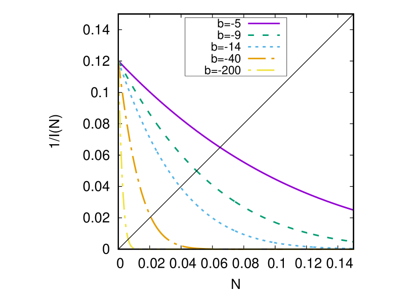
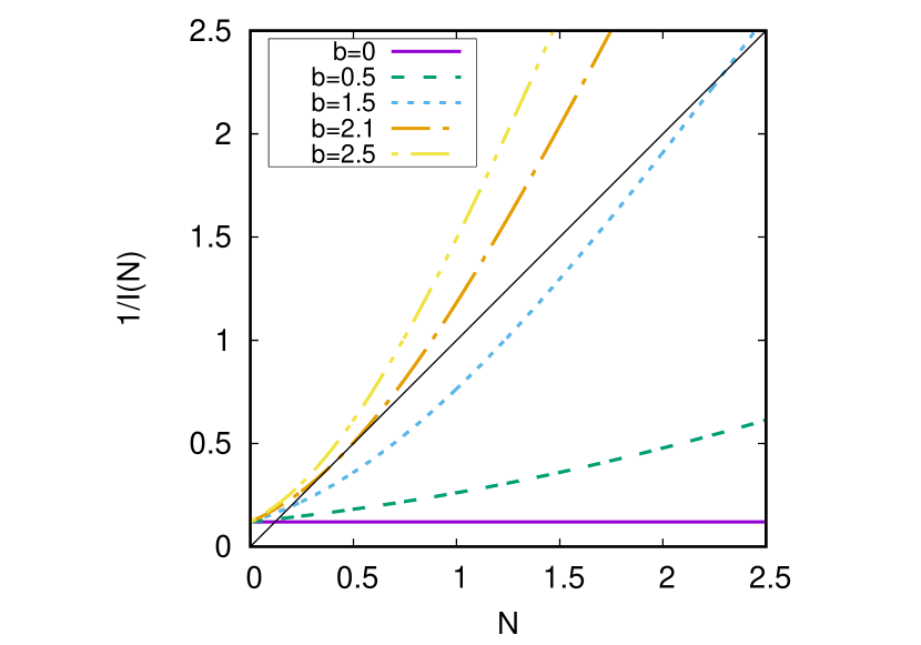
Figure 1: Function $\boldsymbol{\frac{1}{I(N)}}$ (see (1.4)) for different values of the connectivity parameter $\boldsymbol{b}$. Each crossing with the diagonal corresponds to an equilibrium of equation (1.1). Reset and firing potential are set to $V_{R}=1$ and $V_{F}=2$ respectively.

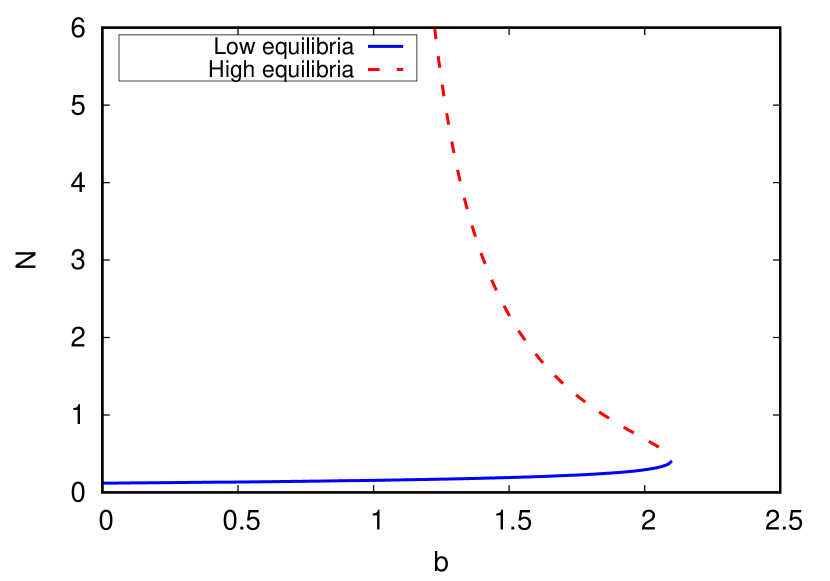
Figure 2: Values of $\boldsymbol{N}$ solving $\boldsymbol{N(I(N))=1,}$ for each $\boldsymbol{b}$. Point $b=1$ corresponds to $b=V_{F}-V_{R}$ for the selected parameter values. Therefore, there is only one equilibrium for $b<1$, two equilibria for $1<b<b_{e}$ with $b_{e}$ a certain critical value, and none for $b>b_{e}$. The dashed line has a vertical asymptote at $b=1$. Reset and firing potential are set to $V_{R}=1$ and $V_{F}=2$ respectively.

Existence theory for NNLIF models has been developed in [15, 5, 13, 11, 12, 10, 47]. In [15] an existence criterion for the nonlinear system (1.1) without delay ($d=0$) was given: the solution exists as long as the firing rate $N(t)$ remains finite. The authors proved that for $d=0$ and $b<0$ (average-inhibitory case) solutions are global in time, while for $b>0$ a blow-up phenomenon (the firing rate $N_{p}(t)$ diverges in finite time) may appear if the initial condition is concentrated near the threshold potential $V_{F}$ [5], or if a large connectivity parameter $b$ is considered [47]. In that case, solutions are not globally defined for all times. The blow-up phenomenon disappears if some transmission delay is taken into account, i.e. if $d>0$, leading to global existence as proved in [10]. Blow-up may also be avoided by considering a stochastic discharge potential [8].

At the microscopic scale analogous criteria for existence and blow-up phenomena were studied in [22]. For the corresponding SDE the notion of solution was extended to the notion of physical solutions in [21]. Physical solutions continue after system synchronization, this is after the blow-up phenomenon, and therefore, they are global in time. In [9], the particle system was analysed numerically to understand the meaning of physical solutions for the Fokker-Planck equation (1.1). However, the analytical study is still an open problem.

This article is devoted to the study of the long-term behavior of system (1.1). Here is an up-to-date summary of its expected behavior, for which there is strong numerical evidence [4, 5, 9, 12, 33, 7, 32], but only few proofs are available:

1. There is some $b_{e}>0$ such that for $b>b_{e}$ no equilibria exist [5]. In this case, solutions without delay ($d=0$) are expected to always blow-up [47]. Solutions with positive delay $d>0$ (which cannot blow-up) are expected to converge as $t\to+\infty$ to the plateau distribution (the uniform distribution on $[V_{R},V_{F}]$ [9].

2. For $V_{F}-V_{R}<b<b_{e}$ two equilibria exist (in [5] it was proved that at least two exist). The higher equilibrium (the one with higher associated firing rate) is unstable for any delay $d\geq 0$ and the lower equilibrium (the one with lower firing rate) is asymptotically stable for any delay $d\geq 0$. Depending on the initial condition $p_{0}$, solutions either converge to the lower equilibrium, blow-up (only possible with $d=0$), or converge to the plateau distribution (only possible when $d>0$).

3. For $0<b<V_{F}-V_{R}$ the unique equilibrium is asymptotically stable regardless of delay. Solutions either converge to this unique equilibrium, or blow-up (only possible if $d=0$ [5]).

4. There is a critical value $b_{p}<0$ such that for any $b_{p}<b<0$, the unique equilibrium is asymptotically stable for all values of the delay. All solutions are expected to converge to this unique equilibrium, independently of the delay.

5. For $b<b_{p}$, there is also a unique equilibrium.

   1. For small values of the delay, this equilibrium is stable. All solutions are expected to converge towards it.

   2. For large values of the delay the equilibrium is unstable. All solutions are expected to approach a periodic solution.

We emphasize that the above statements are on expected behavior, and they are not proved in many cases. Let us also give a summary of rigorous results on asymptotic behavior. In the linear case ($b=0$) [5] proved that solutions converge exponentially fast to the unique steady state. In the quasi-linear case ($|b|$ small), the same is proved in [13] if the initial condition is close enough to the equilibrium. These results were proved by means of the entropy dissipation method, considering the relative entropy functional between the solution $p$ and the stationary solution $p_{\infty}$, given by

$$H(p|p_{\infty}):=\int_{-\infty}^{V_{F}}\frac{\left(p(v,t)-p_{\infty}(v)\right)^{2}}{p_{\infty}(v)}\,\mathrm{d}v=\|p-p_{\infty}\|_{L^{2}(p_{\infty}^{-1})}.$$

It is also known rigorously that there are no periodic solutions if $b$ is large enough, $V_{F}\leq 0$ and a transmission delay is considered [10, 47].

There is strong evidence for the existence of periodic solutions (point 5(b)), according to the approximated model studied in [33], and these periodic solutions are clearly seen numerically. In this paper we are able to map the region where periodic solutions are expected; see Figure 4. For the complete model including different populations of excitatory and inhibitory neurons, considering neurons with refractory periods, as well as the stochastic discharge potential model, the numerical results in [12, 8] also show periodic solutions.

In a companion article to this one [7], we numerically show the close relationship between a discrete sequence of pseudo equilibria and the long term behaviour of the nonlinear system with large delays, with some further analytical results for small $|b|$. This link gives further evidence for the expected behavior described above in 1-5 (in the case of large delay $d$).

Applications of entropy methods have only given results for weakly connected networks (small $b$) so far, i.e. almost linear systems. Building on these results, in this article we give further properties of the linear operator and extend some of them to the linearization of the PDE (1.1). We can thus obtain results about its long term behavior using a different approach that does not require the connectivity parameter $b$ to be small. Here is a summary of the results we show in this paper for solutions to (1.1):

1. We give a new proof that, for small $|b|$, the (unique) equilibrium is stable. Our proof works for a given small $|b|$, and any delay $d\geq 0$; this should be compared to [10], where a condition on $d$ was needed. See Section 4.1 for a precise statement. The proof we present here is also different from the one, mentioned above, that we proved in [7] by pseudo equilibria sequence.

2. With a similar proof, in Section 4.2 we show that linearized stability of an equilibrium implies its nonlinear stability without delay, which is a new result as far as we know. We expect the same to be true also for any positive delay, but the proof runs into technical difficulties that we have not been able to overcome.

3. More importantly, we give explicit criteria to study whether a given equilibrium is linearly stable or not. These criteria are intimately related to the slope at which the curve $N\mapsto(I(N))^{-1}$ crosses the diagonal in Figure 1, which also determines the behaviour of the firing rate sequence, which provides the pseudo equilibria sequence (see [7] for more details).

Point 3 is in our opinion the most surprising one, since it gives a rather complete picture of the asymptotic behavior of the PDE (1.1). In order to state more precisely our theorem regarding point 3 we need to introduce a few definitions. First, given a fixed $N\geq 0$ and $b\in\mathbb{R}$ we define the linear operator $L_{N}$, acting on functions $u=u(v)$, by

$$L_{N}u:=\partial^{2}_{v}u+\partial_{v}((v-bN)u)+\delta_{V_{R}}N_{u}.$$ (1.5)

This operator is formally obtained by replacing $N_{p}$ on the nonlinear term in the right hand side of (1.1a) by $N$. The associated linear PDE,

$$\partial_{t}p=L_{N}p,$$ (1.6)

with the same Dirichlet boundary condition as before and $N_{u}(t):=-\partial_{v}u(V_{F},t)$, models a situation where neurons evolve with a fixed background firing rate. A central part of our strategy is based on a careful study of the linear operator $L_{N}$. The PDE (1.6) has a unique (probability) stationary state $p_{\infty}$, explicitly given by a very similar expression to (1.3):

$$p_{\infty}^{N}(v)=\overline{N}e^{-\frac{\left(v-bN\right)^{2}}{2}}\int_{\max(v,V_{R})}^{V_{F}}e^{\frac{\left(w-bN\right)^{2}}{2}}\,\mathrm{d}w,$$ (1.7)

where $\overline{N}$ is a normalizing factor to ensure that $p_{\infty}^{N}$ is a probability distribution. It is also known that solutions to this linear equation converge exponentially to equilibrium in the weighted norm $L^{2}(1/p_{\infty})$, which is a natural norm when considering a quadratic entropy [5, 13]. By studying some well-posedness and regularization bounds for the linear equation, we are able to show that this exponential decay is also true in the smaller space $X$ given by

$$X:=\{u\in\mathcal{C}(-\infty,V_{F}]\cap\mathcal{C}^{1}(-\infty,V_{R}]\cap\mathcal{C}^{1}[V_{R},V_{F}]\mid u(V_{F})=0\ \text{and}\ \|u\|_{X}<\infty\},$$ (1.8)

where

$$\|u\|_{X}:=\|u\|_{\infty}+\|\partial_{v}u\|_{\infty}+\|u\|_{L^{2}(\varphi)}+\|\partial_{v}u\|_{L^{2}(\varphi)}$$ (1.9)

and

$$\varphi(v):=\exp\left(\frac{(v-bN)^{2}}{2}\right),\qquad v\in(-\infty,V_{F}].$$

It is understood that the $L^{2}(\varphi)$ norms are taken on $(-\infty,V_{F}]$. The linear space $X$ is a Banach space with the above norm. We observe that $X\subseteq L^{2}((p_{\infty}^{N})^{-1})$ since for some constant $C>0$

$$\frac{1}{p_{\infty}^{N}(v)}=C\varphi(v)\qquad\text{for all $v\leq V_{R}$,}$$ (1.10)

and for any $u\in X$ we have

$$\int_{V_{R}}^{V_{F}}u(t,v)^{2}p_{\infty}^{N}(v)^{-1}\,\mathrm{d}v\lesssim\int_{V_{R}}^{V_{F}}u(t,v)^{2}\frac{1}{V_{F}-v}\,\mathrm{d}v\\ \leq\|\partial_{v}u(\cdot,t)\|_{\infty}^{2}\int_{V_{R}}^{V_{F}}(V_{F}-v)\,\mathrm{d}v\lesssim\|u\|_{X}^{2},$$ (1.11)

where we have used the estimate

$$|u(t,v)|\leq\|\partial_{v}u(t,\cdot)\|_{\infty}(V_{F}-v)\qquad\text{for $v\leq V_{F}$,}$$

easily obtained via the mean value theorem and the fact that $u(V_{F})=0$. Inequalities (1.10) and (1.11) show that $\|u\|_{L^{2}(p_{\infty}^{-1})}\lesssim\|u\|_{X}$, so $X\subseteq L^{2}(p_{\infty}^{-1})$.

The property that the linear PDE decays exponentially to equilibrium in a certain space is often stated by saying that it has a spectral gap in that space. The technique we use to “shrink” the space where a given linear PDE has a spectral gap was used in [18] in relation to a coagulation-fragmentation PDE, and is linked to operator techniques described in [31] and [36]. A spectral gap in the space $X$ allows us to carry out stability arguments in a more natural way, since now the firing rate $N_{p}$, considered as an operator $-\partial_{v}p(V_{F})$ acting on $p$, is a bounded linear operator on $X$. This allows us to relate the linearized and the nonlinear equations, and to give more precise estimates on the range of parameters where stability or instability take place.

Given $b\in\mathbb{R}$ and a probability equilibrium $p_{\infty}$ of the PDE (1.1), we call $N_{\infty}:=-\partial_{v}p_{\infty}(V_{F})$ the equilibrium firing rate, and we define the linearized equation at $p_{\infty}$ by

$$\partial_{t}u= \partial^{2}_{v}u+\partial_{v}((v-bN_{\infty})u)+\delta_{V_{R}}N_{u}-bN_{u}(t-d)\partial_{v}p_{\infty}$$ (1.12)

$$= L_{\infty}u-bN_{u}(t-d)\partial_{v}p_{\infty},$$

where $L_{\infty}\equiv L_{N_{\infty}}$ is the linear operator from (1.5), with $N=N_{\infty}$. We notice that this equation has a delay $d$ in the last term. We add the same boundary condition as before, that is,

$$u(V_{F},t)=0,\qquad\text{for $t>0$.}$$ (1.13)

Definition 1.1.

Take $b\in\mathbb{R}$ and $d\geq 0$. We say that a probability equilibrium $p_{\infty}$ of system (1.1) is linearly stable if there exist $C\geq 1$ and $\lambda>0$ such that all solutions $u$ to the linearized equation (1.12)–(1.13) with an initial condition $u_{0}\in\mathcal{C}([-d,0];X)$ such that

$$\int_{-\infty}^{0}u_{0}(v,t)\,\mathrm{d}v=0\qquad\text{for all $t\in[-d,0]$}$$ (1.14)

satisfy

$$\|u(\cdot,t)\|_{X}\leq Ce^{-\lambda t}\sup_{\tau\in[-d,0]}\|u_{0}(\cdot,\tau)\|_{X}\qquad\text{for all $t\geq 0$.}$$ (1.15)

We say that $p_{\infty}$ is linearly unstable if this is not true for $\lambda=0$ and any $C\geq 1$; that is, if for any $C\geq 1$ there exists $u_{0}$ satisfying (1.14) and $t>0$ such that

$$\|u(\cdot,t)\|_{X}\geq C\sup_{\tau\in[-d,0]}\|u_{0}(\cdot,\tau)\|_{X}.$$

For the rest of the paper, whenever $p_{\infty}$ is an equilibrium of the nonlinear problem, we define

$$q(v,t):=e^{tL_{\infty}}\partial_{v}p_{\infty},$$ (1.16)

where $e^{tL_{\infty}}$ denotes the flow of the linear problem (1.5) (that is: $e^{tL_{\infty}}u_{0}$ is the solution to problem (1.5) with initial condition $u_{0}$). In agreement with our previous notation we set

$$N_{q}(t):=-\partial_{v}q(V_{F},t),\qquad\text{for $t>0$,}$$ (1.17)

and call $\hat{N}_{q}$ the Laplace transform of $N_{q}$,

$$\hat{N}_{q}(\xi):=\int_{0}^{\infty}e^{-\xi t}N_{q}(t)\,\mathrm{d}t.$$ (1.18)

We prove in Section 2 that $|N_{q}(t)|\leq Ce^{-\lambda t}$ for some $C,\lambda>0$, and hence $\hat{N}_{q}(\xi)$ is well defined for $\Re(\xi)>-\lambda$. Here is the final theorem that we are able to prove in Section 5:

Theorem 1.2.

Take $b\in\mathbb{R}$ and $d\geq 0$, and let $p_{\infty}$ be a (probability) stationary state of system (1.1), and define $\hat{N}_{q}$ by (1.16)–(1.18). The steady state $p_{\infty}$ is linearly stable if and only if all zeros of the analytic function

$$\Phi_{d}(\xi):=1+b\hat{N_{q}}(\xi)\exp(-\xi d)$$

(defined for $\Re(\xi)>-\lambda$) are located on the real negative half-plane $\{\xi\in\mathbb{C}\mid\Re(\xi)<0\}$.

This result simplifies the numerical study of the stability of equilibria, and gives some theoretical consequences. For example, we have:

Corollary 1.3.

Take $b\in\mathbb{R}$. If a probability stationary state $p_{\infty}$ of system (1.1) is linearly stable for $d=0$, then it is linearly stable also for small enough $d>0$.

Proof.

If $p_{\infty}$ is linearly stable for $d=0$, it means that for some $\mu>0$, the function $\Phi_{0}$ does not have any zeros on $\mathbb{C}_{\mu}:=\{\xi\in\mathbb{C}\mid\Re(\xi)\geq-\mu\}$. By properties of the Laplace transform, $\hat{N_{q}}(\xi)$ tends to zero both when $\Im(\xi)\to\pm\infty$ and when $\Re(\xi)\to+\infty$. Hence all possible zeros of $\Phi_{d}$ in $\mathbb{C}_{\mu}$, for any $d\geq 0$, must be in some fixed compact subset $K\subseteq C_{\mu}$. Since the functions $\Phi_{d}$ are continuous and $\Phi_{d}(\xi)\to\Phi_{0}(\xi)$ uniformly as $d\to 0$, we see that for $d$ small, the function $\Phi_{d}$ cannot have any zeros on $K$, and hence cannot have zeros on $\mathbb{C}_{\mu}$. ∎

There is a specific value of $\hat{N}_{q}$ which is linked to the function $I(N)$: in Lemma 5.1 we show that

$$b\hat{N_{q}}(0)=\frac{\mathrm{d}}{\mathrm{d}N}\Big{|}_{N=N_{\infty}}\left(\frac{1}{I(N)}\right).$$

As a consequence, analyzing the zeros of $\Phi_{d}(\xi)$ gives us the following criterion of stability/instability, often easier to check:

Theorem 1.4.

Let us set $V_{R}<V_{F}\in\mathbb{R}$, $b\in\mathbb{R}$, and let $p_{\infty}$ be a probability equilibrium of the nonlinear equation (1.1). Call $N_{\infty}:=-\partial_{v}p_{\infty}(V_{F})$ its associated firing rate.

1. If

   $$\frac{\mathrm{d}}{\mathrm{d}N}\Big{|}_{N=N_{\infty}}\left(\frac{1}{I(N)}\right)>1$$

   then $p_{\infty}$ is a linearly unstable equilibrium, for any delay $d\geq 0$.

2. If

   $$|b|\int_{0}^{\infty}|N_{q}(t)|\,\mathrm{d}t<1$$

   then the equilibrium $p_{\infty}$ is linearly stable, for any delay $d\geq 0$.

3. If

   $$\frac{\mathrm{d}}{\mathrm{d}N}\Big{|}_{N=N_{\infty}}\left(\frac{1}{I(N)}\right)<-1$$ (1.19)

   then the equilibrium $p_{\infty}$ is linearly unstable when the delay $d$ is large enough.

This criterion is also in agreement with the prediction of the pseudo equilibria sequence given in [7] for networks with large transmission delay. It strikes us that the criterion is given in terms of the slope of $\frac{1}{I(N)}$ (see (1.4) for an explicit expression of $I$), which determines the behaviour of the discrete sequence of firing rates studied in [7].

The function $1/I(N)$ is explicit (see (1.4)) and the only obstacle to checking analytically whether the conditions in Theorem 1.4 hold is that the expression of $I(N)$ is cumbersome to work with. Some rigorous properties of $I$ are given in [5, 7], but in any case the following is clearly seen numerically (Figure 1):

• Case 1 in Theorem 1.4 holds in the excitatory case $b>0$, assuming there are two equilibria. The higher equilibrium satisfies $\frac{\mathrm{d}}{\mathrm{d}N}\Big{|}_{N=N_{\infty}}\left(\frac{1}{I(N)}\right)>1$ (with $N_{\infty}$ the highest stationary firing rate). Hence assuming there are two equilibria, the higher equilibrium is unstable.

• Case 2 in Theorem 1.4 seems hard to check analytically, though numerical checks are straightforward. This case takes place for the lower equilibrium if there are two of them, and for the single equilibrium whenever there is a unique one.

• Case 3 in Theorem 1.4 can be rigorously proved to hold when $b<0$ is sufficiently negative. Hence there is some $b^{*}<0$ such that for $b<b^{*}$ and large enough $d>0$, the unique equilibrium $p_{\infty}$ is linearly unstable.

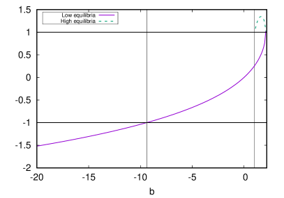
Figure 3: Value of $S(b):=-b\int_{0}^{\infty}N_{q}(t)\,\mathrm{d}t=\frac{\mathrm{d}}{\mathrm{d}N}\Big{|}_{N=N_{\infty}}\left(\frac{1}{I(N)}\right)$ for different values of $b$. Vertical lines at $b=-9.4$ and $b=1$ separate regions with different behaviours in terms of stability for equilibria of equation (5.3): for $b<-9.4$ (one equilibrium) we find that $S(b)<-1$, which coincides with point 3 of Theorem 1.4, i.e. the region of $b$ where equilibria stability depends on the delay value; in the case $-9.4<b<1$ (one equilibrium), we get $|S(b)|=|b|\int_{0}^{\infty}|N_{q}(t)|\,\mathrm{d}t<1$ (since the function $N_{q}(t)$ is numerically seen to be always monotone), leading us to the scenario in point 2 of Theorem 1.4, where regardless of the delay value, the equilibrium is stable. For any $b>1$ there are two equilibria: for the lower equilibrium (solid line) the situation is the same as in the previous case, while for the higher equilibrium (dashed line), $S(b)>1$ and point 1 of Theorem 1.4 is fulfilled. Reset and firing potential are set to $V_{R}=1$ and $V_{F}=2$ respectively.

We note that Theorem 1.4 may not be fully exhaustive. First, because it does not speak about the critical cases where $\frac{\mathrm{d}}{\mathrm{d}N}\Big{|}_{N=N_{\infty}}(1/I(N))=\pm 1$. And second, even ignoring these cases, it may still happen that none of its three possibilities are satisfied. However, from our simulations we suspect that the criterion is in fact exhaustive except at the critical cases, since we expect $N_{q}(t)$ to have a fixed sign for all $t>0$ (which seems clear numerically), and then

$$|b|\int_{0}^{\infty}|N_{q}(t)|\,\mathrm{d}t=\left|\frac{\mathrm{d}}{\mathrm{d}N}\Big{|}_{N=N_{\infty}}\left(\frac{1}{I(N)}\right)\right|.$$

On the other hand, point 3 of Theorem 1.4 does not give information on the case of strongly inhibitory systems with small delay. For those cases we must study the zeros of $\Phi_{d}$, as indicated by Theorem 1.2, and the best we can say is Corollary 1.3.

The stability criteria in Theorem 1.2 and 1.4 can be checked numerically and allow us to give a rather complete picture of the stability of equilibria, including the threshold delay for which the equilibrium becomes unstable, as shown in Figure 4.

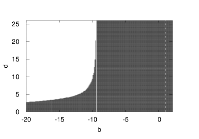
Figure 4: Stability map of the linearized equation. For each pair of values of the connectivity parameter and transmission delay $(b,d)$, this color map shows the stability (dark) or instability (white) for the solutions of the linearized equation (1.12). The vertical black solid line placed at $b_{p}\approx-9.4$ separates the region of unconditional stability (for any delay $d$), from that where stability depends on the value of $d$. The vertical dashed line at $b=1$ separates the region with a unique steady state (left) from the one with two steady states (right). For cases with two steady states (that is, to the right of the vertical dashed line) we consider the lower one. The stability condition considered to make this map is based on Theorems 1.2 and 1.4: for each $b$ we find its related equilibrium $p_{\infty}$, choosing the lower one if there are two equilibria; we differentiate $p_{\infty}$ and use it as initial condition for the linear system given by equation (1.1a), thus obtaining $q(v,t)=e^{tL_{\infty}}\partial_{v}p_{\infty}$ and $N_{q}(t)$. Cases 1 and 2 of Theorem 1.4 account for all cases with $b>b_{p}$. In order to tell apart the cases with $b<b_{p}$, for each $d>0$ we compute $Q(k):=-be^{-ikd}\int_{0}^{\infty}N_{q}(t)e^{ikt}\,\mathrm{d}t$, with $k\in\mathbb{R}$; finally we count the number of times that $Q(k)$ crosses the line $(1,\infty)$ taking into account its orientation. If the net balance of crossings is different from $0$, the equilibrium $p_{\infty}$ related to $(b,d)$ is unstable (see the proof of Theorem 1.4 in Section 5 for a better understanding of this). Otherwise we need to compute the zeros of function $\Phi_{d}(\xi):=1+b\hat{N_{q}}(\xi)\exp(-\xi d)$, given in Theorem 1.2 in order to check whether the equilibrium is stable or not. Reset and firing potential are set to $V_{R}=1$ and $V_{F}=2$ respectively.

Though it is not contained in Theorem 1.4, we point out that the expected behavior of the nonlinear system (1.1) when $(b,d)$ is in the unstable region with $b<0$ should be periodic, as shown consistently in simulations [33, 7]. That is, we expect solutions to converge to a unique (up to time translations) periodic solution with period approximately equal to $2d$. Since the analysis leading to Theorem 1.4 is based on the linearized equation, we are not able to show a global behavior such as periodic solutions, but the mechanism for their appearance seems to be given by the presence of delayed negative feedback: in the literature on delay equations there are many instances of periodic behavior, arising due to a delayed system in which the driving force works against the displacement that the system has seen in the previous delay period. See for example the books [23] (especially chapter XV) or [29] for an exposition of this topic.

Before concluding this introduction it is worth mentioning that other PDE families model the activity of a large number of neurons based on the integrate and fire approach: population density models of integrate and fire neurons with jumps [40, 27, 26, 25]; Fokker-Planck equations for uncoupled neurons [38, 39]; and Fokker-Planck equations including conductance variables [46, 6, 44, 45] There are also closely related models, not strictly of NNLIF type, such as time elapsed models [41, 42, 43] which are derived as mean-field limits of Hawkes processes [20, 19]; McKean-Vlasov equations [1, 37], which are the mean-field equations associated with a large number of Fitzhugh-Nagumo neurons [30]; Nonlinear Fokker-Planck systems which describe networks of grid cells [16, 17] and are rigorously achieved by mean-field limits [14].

The paper is structured as follows: in Section 2 we carry out our study of the linear equation, giving well-posedness and regularization estimates in the space $X$, and showing that the linear PDE has a spectral gap in the space $X$. In Section 3 we lay out some groundwork on classical delay equations, needed for the arguments presented in later sections. In Section 4 we give a result on the nonlinear stability of the NNLIF model for weak interconnectivity, and we show that linearized stability implies nonlinear stability (that is, that linearized behavior dominates close to an equilibrium). Finally, in Section 5 we give a new criterion for linear stability or instability of equilibria with a given connectivity $b$ and delay $d$, which implies corresponding results for the nonlinear equation, due to the results in Section 4.

Throughout the paper we often use $C$ to denote an arbitrary nonnegative constant which may change from line to line. We also use the symbol $\lesssim$ to denote inequality up to a positive multiplicative constant.

2 Study of the linear equation

In this section we study several aspects of the following linear equation, which results when we fix the firing rate $N$, independent on time, in the nonlinear term of equation (1.1):

$$\partial_{t}u(v,t)=\partial_{v}^{2}u(v,t)+\partial_{v}[(v-bN)u(v,t)]+\delta_{V_{R}}N_{u}(t),\ v\in\left(-\infty,V_{F}\right],\ t\geq 0,$$ (2.1a)

with the boundary condition

$$u(V_{F},t)=0,t\geq 0$$ (2.1b)

and defining

$$N_{u}(t):=-\partial_{v}u(V_{F},t).$$ (2.1c)

As usual, we also impose an initial condition at time $$t=0$$:

$$u(v,0)=u_{0}(v),\qquad v\in(-\infty,V_{F}].$$ (2.1d)

We will first study well-posedness bounds in several spaces, and then study its spectral gap properties in suitable “strong” spaces which will later be useful for the nonlinear theory.

2.1 Summary of results: well-posedness, regularity and spectral gap

Let us state our main results on the linear equation, leaving the proof of all technical estimates for Section 2.2. We recall that an existence theory for classical solutions to the nonlinear system (1.1) was given in [15], which covers in particular the linear case (2.1a) (as the case with $b=0$ in their paper). Throughout this section we assume this existence theory, and we develop some more precise well-posedness estimates on these classical solutions. Actually, from our estimates below one could construct a linear existence theory for equation (2.1a) by using known tools from semigroup theory (see [28], in particular Section III.3 and the Desch-Schappacher theorem). We do not follow this path here since we think it is more direct to work with the already studied classical solutions, developing new estimates for them.

We also know from previous results [5] that equation (2.1), in the linear case, has a unique probability equilibrium $p_{\infty}^{N}$ (given by (1.7)), which in this section we denote simply by $p_{\infty}$, since we work only with the linear equation in all of Section 2. This equilibrium is positive, and the linear equation has a spectral gap in the space $L^{2}(p_{\infty}^{-1})$: there exists $\lambda>0$ such that for all probability distributions $p_{0}\in L^{2}(p_{\infty}^{-1})$,

$$\|e^{tL}p_{0}-p_{\infty}\|_{L^{2}(p_{\infty}^{-1})}\leq e^{-\lambda t}\|p_{0}-p_{\infty}\|_{L^{2}(p_{\infty}^{-1})}\qquad\text{for all $t\geq 0$.}$$ (2.2)

In fact, the same reasoning from [5], based on a Poincaré’s inequality, actually shows something slightly stronger: for any initial condition $u_{0}\in L^{2}(p_{\infty}^{-1})$ such that $\int_{-\infty}^{V_{F}}u_{0}(v)\,\mathrm{d}v=0$ we have

$$\|e^{tL}u_{0}\|_{L^{2}(p_{\infty}^{-1})}\leq e^{-\lambda t}\|u_{0}\|_{L^{2}(p_{\infty}^{-1})}\qquad\text{for all $t\geq 0$.}$$ (2.3)

Another straightforward consequence is that there exists $C\geq 1$ such that for any $u_{0}\in L^{2}(p_{\infty}^{-1})$ (not necessarily with integral $0$) we have

$$\|e^{tL}u_{0}\|_{L^{2}(p_{\infty}^{-1})}\leq C\|u_{0}\|_{L^{2}(p_{\infty}^{-1})}\qquad\text{for all $t\geq 0$.}$$ (2.4)

Due to (2.3), this is clearly true (with $C=1$) if $u_{0}$ has integral $0$. For a general $u_{0}\in L^{2}(p_{\infty}^{-1})$, (2.4) may be obtained by writing $u_{0}=(u_{0}-mp_{\infty})+mp_{\infty}$, with $m:=\int_{-\infty}^{V_{F}}u_{0}(v)\,\mathrm{d}v$, applying (2.3), and noticing that $|m|\leq C\|u_{0}\|_{L^{2}(p_{\infty}^{-1})}$ for some $C>0$:

$$\|e^{tL}u_{0}\|_{L^{2}(p_{\infty}^{-1})}\leq\|e^{tL}(u_{0}-mp_{\infty})\|_{L^{2}(p_{\infty}^{-1})}+|m|\|e^{tL}p_{\infty}\|_{L^{2}(p_{\infty}^{-1})}\\ \leq e^{-\lambda t}\|u_{0}-mp_{\infty}\|_{L^{2}(p_{\infty}^{-1})}+|m|\|p_{\infty}\|_{L^{2}(p_{\infty}^{-1})}\\ \leq\|u_{0}\|_{L^{2}(p_{\infty}^{-1})}+|m|\|p_{\infty}\|_{L^{2}(p_{\infty}^{-1})}+|m|\|p_{\infty}\|_{L^{2}(p_{\infty}^{-1})}\\ \leq(1+2C\|p_{\infty}\|_{L^{2}(p_{\infty}^{-1})})\|u_{0}\|_{L^{2}(p_{\infty}^{-1})}.$$

Our main aim is to have good estimates, similar to (2.3) and (2.4), in a linear space where the derivative of the solution is bounded (unlike $L^{2}(p_{\infty}^{-1})$). We consider the space $X$ defined in (1.8) (associated to the unique probability equilibrium $p_{\infty}$ of (2.1)). Here are the main estimates we wish to prove on this:

Lemma 2.1 (Well-posedness estimate).

Let $u_{0}\in X$ be any initial condition. Then the solution $u$ to the linear equation (2.1) satisfies the following: there are constants $M,C>0$ such that

$$\|e^{tL}u_{0}\|_{X}\leq Me^{Ct}\|u_{0}\|_{X}\qquad\text{for all $t\geq 0$.}$$ (2.5)

And here is our main regularization estimate:

Lemma 2.2 (Regularization estimate).

Let $u_{0}\in X$ be any initial condition. Then the solution $u$ to the linear equation (2.1) satisfies the following: there exists a constant $C>0$ and $t_{0}>0$ (both independent of the initial condition $u_{0}$), such that

$$\|e^{tL}u_{0}\|_{X}\leq Ct^{-3/4}\|u_{0}\|_{L^{2}(\varphi)}\qquad\text{for all $0<t\leq t_{0}$.}$$ (2.6)

and in particular

$$\|e^{tL}u_{0}\|_{X}\leq Ct^{-3/4}\|u_{0}\|_{L^{2}(p_{\infty}^{-1})}\qquad\text{for all $0<t\leq t_{0}$.}$$ (2.7)

Both of the lemmas above are a direct consequence of the bounds in Lemmas 2.11 and 2.12, proved at the end of Section 2.2. Notice that

$$\varphi(v)\lesssim\frac{1}{p_{\infty}(v)}\qquad\text{for all $v<V_{F}$},$$

so (2.7) is clearly a consequence of (2.6).

Regarding spectral gap estimates, we show that the semigroup associated to the linear equation has a spectral gap in the space $X$. This is essentially deduced from the known spectral gap estimate (2.3) and Lemmas 2.1 and 2.2:

Proposition 2.3 (Spectral gap estimate).

There exist constants $\lambda>0$, $C\geq 1$ such that for all initial conditions $u_{0}\in X$ such that $\int_{-\infty}^{V_{F}}u_{0}(v)\,\mathrm{d}v=0$ it holds that

$$\|e^{tL}u_{0}\|_{X}\leq Ce^{-\lambda t}\|u_{0}\|_{X}\qquad\text{for all $t\geq 0$}$$ (2.8)

and also

$$\|e^{tL}u_{0}\|_{X}\leq Ct^{-\frac{3}{4}}e^{-\lambda t}\|u_{0}\|_{L^{2}(\varphi)}\qquad\text{for all $t>0$.}$$ (2.9)

Remark 2.4.

From the proof below one can see that the constant $\lambda$ in (2.8) can be taken to be the same one as in (2.2) (usually obtained via a Poincaré’s inequality [5]). The constant $\lambda$ in (2.9) can be taken to be any constant strictly smaller than the $\lambda$ in (2.2) (or alternatively, one could keep the same $\lambda$ and write $\max\{1,t^{-3/4}\}$ instead of $t^{-3/4}$ in (2.9)).

Proof.

Call $Y\equiv L^{2}(p_{\infty}^{-1})$. Our regularization result in equation (2.7) gives

$$\|e^{tL}u_{0}\|_{X}\lesssim t^{-\frac{3}{4}}\|u_{0}\|_{Y}\qquad\text{for all $0<t\leq t_{0}$.}$$

Now we can prove (2.8) for $t\geq t_{0}$ by using (2.3): for $t\geq t_{0}$ we have

$$\|e^{tL}u_{0}\|_{X}=\|e^{t_{0}L}e^{(t-t_{0})L}u_{0}\|_{X}\lesssim t_{0}^{-\frac{3}{4}}\|e^{(t-t_{0})L}u_{0}\|_{Y}\\ \lesssim t_{0}^{-\frac{3}{4}}e^{-\lambda(t-t_{0})}\|u_{0}\|_{Y}\lesssim t_{0}^{-\frac{3}{4}}e^{-\lambda(t-t_{0})}\|u_{0}\|_{X}\lesssim e^{-\lambda t}\|u_{0}\|_{X}.$$

Notice that we also used $\|u_{0}\|_{Y}\lesssim\|u_{0}\|_{X}$, since $X\subseteq Y$ (see the observation after (1.9) in the introduction). For $t\leq t_{0}$ we can use the well-posedness estimate of Lemma 2.1, finally getting (2.8) for all $t\geq 0$.

In order to show (2.9) we take any $t>0$ and any $0<s<\min\{t_{0},t\}$, and we use (2.8) and (2.6) to write

$$\|e^{tL}u_{0}\|_{X}=\|e^{(t-s)L}e^{sL}u_{0}\|_{X}\lesssim e^{-\lambda(t-s)}\|e^{sL}u_{0}\|_{X}\lesssim s^{-\frac{3}{4}}e^{-\lambda(t-s)}\|u_{0}\|_{L^{2}(\varphi)}.$$

For $t\geq t_{0}$ we take $s:=t_{0}/2$ and this shows (2.9) (with a slightly smaller $\lambda$). For $t<t_{0}$ we take $s=t/2$, and this also gives the result on that range. ∎

2.2 Bounds for classical solutions

In order to study the linear equation (2.1a) we separate its terms as follows

$$\partial_{t}u=\partial_{v}^{2}u+\partial_{v}[(v-bN)u]+\delta_{V_{R}}N_{u}(t)=Fu+L_{1}u+L_{2}u,$$ (2.10)

with

$$Fu:=\partial_{v}^{2}u+\partial_{v}[(v-V_{F})u],\qquad L_{1}u:=\delta_{V_{R}}N_{u}(t),\qquad L_{2}u:=\partial_{v}[(V_{F}-bN)u].$$

We still consider the same boundary conditions (2.1b). In order, we prove estimates for the equation $\partial_{t}u=Fu$ in Section 2.2.1, then for $\partial_{t}u=Fu+L_{1}u$ in Section 2.2.2, and finally for the full linear equation in Section 2.2.3.

2.2.1 Bounds for the Fokker-Planck equation

The Cauchy problem for the Dirichlet Fokker-Planck equation on the half-line, posed for $t\geq 0$ and $v\in(-\infty,0]$,

$$\partial_{t}u=\partial_{v}^{2}u+\partial_{v}(vu)\qquad\text{with}\qquad u(0,t)=0\quad\text{for $t\geq 0$},$$ (2.11)

$$u(v,0)=u_{0}\qquad\text{with}\qquad u_{0}\colon(-\infty,0]\to\mathbb{R},$$

has the explicit solution

$$u(v,t)=\int_{-\infty}^{\infty}\widetilde{u}_{0}(w)\Phi_{t}(v,w)\,\mathrm{d}w=\int_{-\infty}^{0}u_{0}(w)\Psi_{t}(v,w)\,\mathrm{d}w,$$ (2.12)

defined for $t>0$ and $v\in(-\infty,0]$. Here $\widetilde{u}_{0}\colon\mathbb{R}\to\mathbb{R}$ is the anti-symmetrization of the initial condition

$$\widetilde{u}_{0}(x):=\begin{cases}u_{0}(x),\qquad&x\leq 0\\ -u_{0}(-x),\qquad&x>0,\end{cases}$$

$\Phi_{t}=\Phi_{t}(v,w)$ is the fundamental solution of the standard Fokker-Planck equation:

$$\Phi_{t}(v,w)=\frac{1}{\sqrt{2\pi(1-e^{-2t})}}\exp\left({-\frac{(v-e^{-t}w)^{2}}{2\left(1-e^{-2t}\right)}}\right),\qquad t>0,\quad v,w\in\mathbb{R},$$ (2.13)

and

$$\Psi_{t}(v,w):=\Phi_{t}(v,w)-\Phi_{t}(v,-w),\qquad t>0,\ v,w\in(-\infty,0].$$ (2.14)

For later reference, we notice that $\Psi_{t}(v,w)\geq 0$, since $t>0$ and $v,w\in(-\infty,0]$, and

$$\partial_{v}\Phi_{t}(v,w)=(2\pi)^{-\frac{1}{2}}(1-e^{-2t})^{-\frac{3}{2}}(v-e^{-t}w)\exp\left({-\frac{(v-e^{-t}w)^{2}}{2\left(1-e^{-2t}\right)}}\right).$$ (2.15)

For an explicit solution to be available it is essential that the boundary condition is set at $v=0$; otherwise we do not know of an explicit expression. From the expression (2.12) of the solution, it is easy to see that many estimates for the standard Fokker-Planck equation on $\mathbb{R}$ can be carried over to the Fokker-Planck equation (2.11), posed on $(-\infty,0]$ and with a Dirichlet boundary condition.

It is then straightforward to translate equation (2.12) and obtain a solution to the translated Fokker-Planck equation

$$\partial_{t}u=Fu=\partial_{v}^{2}u+\partial_{v}[(v-V_{F})u]$$ (2.16)

posed for $t\geq 0$ and $v\in(-\infty,V_{F}]$ with the boundary condition

$$u(V_{F},t)=0,\qquad t\geq 0.$$ (2.17)

A solution to (2.16)–(2.17), with initial condition $u_{0}$, is then given by

$$u(v,t)=\int_{-\infty}^{\infty}\widetilde{u}_{0}(w)\Phi_{t}(v-V_{F},w-V_{F})\,\mathrm{d}w=\int_{-\infty}^{V_{F}}u_{0}(w)\Psi_{t}(v-V_{F},w-V_{F})\,\mathrm{d}w,$$ (2.18)

for $t>0$ and $v\in(-\infty,V_{F}]$, where $\widetilde{u}_{0}$ is now the function

$$\widetilde{u}_{0}(x):=\begin{cases}u_{0}(x),\qquad&x\leq V_{F}\\ -u_{0}(2V_{F}-x),\qquad&x>V_{F}.\end{cases}$$

With this explicit expression we can obtain the following estimates:

Lemma 2.5.

Denote by $e^{tF}u_{0}$ the solution (2.18) to the Fokker-Planck equation (2.16)–(2.17) in the domain $v\in(-\infty,V_{F}]$, $t\geq 0$, with an initial condition $u_{0}$. Then, the following well-posedness inequalities hold for all $u_{0}\in X$ and all $t\geq 0$:

$$\|e^{tF}u_{0}\|_{\infty} \leq e^{t}\|u_{0}\|_{\infty}.$$ (2.19)

$$\|e^{tF}u_{0}\|_{2} \leq\sqrt{2}e^{\frac{t}{2}}\|u_{0}\|_{2}.$$ (2.20)

$$\|\partial_{v}e^{tF}u_{0}\|_{\infty} \leq e^{2t}\|\partial_{v}u_{0}\|_{\infty}.$$ (2.21)

$$\|\partial_{v}e^{tF}u_{0}\|_{2} \leq\sqrt{2}e^{\frac{3t}{2}}\|\partial_{v}u_{0}\|_{2}.$$ (2.22)

Also, the following “regularization” inequalities hold for some constants $C>0$, all $u_{0}\in X$ and $t$ small enough:

$$\|e^{tF}u_{0}\|_{\infty} \leq Ct^{-1/4}\|u_{0}\|_{2}.$$ (2.23)

$$\|\partial_{v}e^{tF}u_{0}\|_{\infty} \leq Ct^{-1/2}\|u_{0}\|_{\infty}.$$ (2.24)

$$\|\partial_{v}e^{tF}u_{0}\|_{\infty} \leq Ct^{-3/4}\|u_{0}\|_{2}.$$ (2.25)

$$\|\partial_{v}e^{tF}u_{0}\|_{2} \leq Ct^{-1/2}\|u_{0}\|_{2}.$$ (2.26)

$$\|\partial_{v}e^{tF}u_{0}\|_{\infty} \leq Ct^{-1/4}\|\partial_{v}u_{0}\|_{2}.$$ (2.27)

Proof.

These estimates are obtained in a straightforward way from the explicit solution (2.18), and are a consequence of the corresponding estimates for the standard Fokker-Planck equation on $\mathbb{R}$. We use the standard properties

$$\int_{-\infty}^{+\infty}\Phi_{t}(v,w)\,\mathrm{d}v=1,\qquad\int_{-\infty}^{+\infty}\Phi_{t}(v,w)\,\mathrm{d}w=e^{t}$$ (2.28)

and

$$\int_{-\infty}^{+\infty}(\Phi_{t}(v,w))^{2}\,\mathrm{d}w=\frac{1}{2\sqrt{\pi}}(1-e^{-2t})^{-\frac{1}{2}}e^{t}.$$ (2.29)

In order to obtain (2.19), we directly apply the second part of (2.28) to the expression (2.18). To obtain (2.20) from (2.18) we use the Cauchy-Schwarz inequality and the second part of (2.28) to get

$$\left(\int_{-\infty}^{\infty}\widetilde{u}_{0}(w)\Phi_{t}(v-V_{F},w-V_{F})\,\mathrm{d}w\right)^{2}\\ \leq\left(\int_{-\infty}^{\infty}\widetilde{u}_{0}(w)^{2}\Phi_{t}(v-V_{F},w-V_{F})\,\mathrm{d}w\right)\left(\int_{-\infty}^{\infty}\Phi_{t}(v-V_{F},w-V_{F})\,\mathrm{d}w\right)\\ =e^{t}\left(\int_{-\infty}^{\infty}\widetilde{u}_{0}(w)^{2}\Phi_{t}(v-V_{F},w-V_{F})\,\mathrm{d}w\right).$$ (2.30)

Integrating now in $v$ and taking into account that $\|\widetilde{u_{0}}\|_{2}^{2}=2\|u_{0}\|_{2}^{2}$ gives (2.20).

For the estimates involving the derivative $\partial_{v}$ we note that

$$\partial_{v}\Phi_{t}(v,w)=-e^{t}\partial_{w}\Phi_{t}(v,w).$$ (2.31)

Using this, to obtain (2.21) we write

$$\partial_{v}u(v,t)=\int_{-\infty}^{\infty}\widetilde{u}_{0}(w)\partial_{v}\Phi_{t}(v-V_{F},w-V_{F})\,\mathrm{d}w\\ =e^{t}\int_{-\infty}^{\infty}\partial_{w}\widetilde{u}_{0}(w)\Phi_{t}(v-V_{F},w-V_{F})\,\mathrm{d}w,$$ (2.32)

and now take the supremum of both sides and use the second part of (2.28). We can also obtain (2.22) from this same expression by using a very similar argument as in (2.30).

Regarding the regularization estimates, in order to show $\|e^{tF}u_{0}\|_{\infty}\leq Ct^{-1/4}\|u_{0}\|_{2}$, i.e. (2.23), from (2.18) we easily get

$$\|e^{tF}u_{0}\|_{\infty}\leq\sqrt{2}\|u_{0}\|_{2}\|\Phi_{t}(v,\cdot)\|_{2},$$

and using (2.29) gives (2.23). To show (2.24), we take the supremum in the first expression of equation (2.32) and use the estimate

$$\int_{-\infty}^{+\infty}\left|\partial_{v}\Phi_{t}(v,w)\right|\,\mathrm{d}w=\frac{\sqrt{2}e^{t}}{\sqrt{\pi(1-e^{-2t})}}\int_{-\infty}^{+\infty}|z|e^{-z^{2}}\,\mathrm{d}z\lesssim Ct^{-\frac{1}{2}}\qquad\text{for $0<t\leq 1$.}$$ (2.33)

To prove $\|\partial_{v}e^{tF}u_{0}\|_{\infty}\leq Ct^{-3/4}\|u_{0}\|_{2}$, i.e. (2.25), we use (2.32) to write

$$\|\partial_{v}e^{tF}u_{0}\|_{\infty}\leq e^{t}\sqrt{2}\|u_{0}\|_{2}\|\partial_{v}\Phi_{t}(v,\cdot)\|_{2}.$$

The fact that

$$\int_{-\infty}^{+\infty}(\partial_{v}\Phi_{t}(v,w))^{2}\,\mathrm{d}w=\frac{\sqrt{2}}{\pi}e^{t}(1-e^{-t})^{-\frac{3}{2}}\int_{-\infty}^{+\infty}z^{2}e^{-2z^{2}}\,\mathrm{d}z$$ (2.34)

now shows (2.25). To prove $\|\partial_{v}e^{tF}u_{0}\|_{2}\leq Ct^{-1/2}\|u_{0}\|_{2}$, i.e. (2.26), we use the Cauchy-Schwarz inequality in (2.32) in a similar way as in equation (2.30) to get

$$\|\partial_{v}e^{tF}u_{0}\|_{2}\leq Ce^{\frac{t}{2}}t^{-\frac{1}{4}}\left(\int_{-\infty}^{\infty}\int_{-\infty}^{\infty}\widetilde{u}_{0}(w)^{2}|\partial_{v}\Phi_{t}(v-V_{F},w-V_{F})|\,\mathrm{d}v\,\mathrm{d}w\right)^{\frac{1}{2}},$$

where we also used (2.33). Now the bound

$$\int_{-\infty}^{\infty}|\partial_{v}\Phi_{t}(v,w)|\,\mathrm{d}v=\frac{\sqrt{2}}{\sqrt{\pi(1-e^{-2t})}}\int_{-\infty}^{+\infty}|z|e^{-z^{2}}\,\mathrm{d}z\lesssim Ct^{-\frac{1}{2}}\qquad\text{for $0<t\leq 1$}$$

completes the proof of (2.26). Finally, to prove (2.27), i.e. $\|\partial_{v}e^{tF}u_{0}\|_{\infty}\leq Ct^{-1/4}\|\partial_{v}u_{0}\|_{2}$, we take the supremum in the last expression of (2.32), apply the Cauchy-Schwarz inequality, and then use (2.29). ∎

We also need some additional weighted $L^{2}$ well-posedness and regularization estimates with Gaussian weight, which we state separately here:

Lemma 2.6 ($L^{2}$ Gaussian estimates for the Fokker-Planck equation).

Take $v_{0}\in\mathbb{R}$ and let $\varphi(v):=\exp((v-v_{0})^{2}/2)$. There exist $t_{0}>0$ and $C>0$ depending only on $v_{0}$ and $V_{F}$ such that

$$\|\partial_{v}e^{tF}u_{0}\|_{L^{2}(\varphi)}\leq C\|\partial_{v}u_{0}\|_{L^{2}(\varphi)}\qquad\text{for all $0<t\leq t_{0}$,}$$ (2.35)

and

$$\|\partial_{v}e^{tF}u_{0}\|_{L^{2}(\varphi)}\leq Ct^{-1/2}\|u_{0}\|_{L^{2}(\varphi)}\qquad\text{for all $0<t\leq t_{0}$,}$$ (2.36)

both for any $u_{0}\in X$.

Remark 2.7.

Of course, estimate (2.35) (which has the same norm on both sides) can be iterated for later times to obtain

$$\|\partial_{v}e^{tF}u_{0}\|_{L^{2}(\varphi)}\leq Ce^{\sigma t}\|\partial_{v}u_{0}\|_{L^{2}(\varphi)}\qquad\text{for all $t\geq 0$}$$

for some (other) $C>0$ and some $\sigma>0$. We have chosen to state this kind of estimates only for a short time when we have no straightforward estimate on $\sigma$.

Proof of Lemma 2.6.

Proof of the first estimate when $v_{0}=0$. By possibly changing $v_{0}$ it is enough to write the proof for $V_{F}=0$. We will first prove the result also assuming that $v_{0}=0$, and then point out the modifications needed to obtain the general case. Call $u(\cdot,t)=e^{tF}u_{0}$. From (2.18) we have

$$\partial_{v}u(v,t)=\int_{-\infty}^{0}u_{0}(w)\partial_{v}\Psi_{t}(v,w)\,\mathrm{d}w\\ =-e^{t}\int_{-\infty}^{0}u_{0}(w)\partial_{w}(\Phi_{t}(v,w)+\Phi_{t}(v,-w))\,\mathrm{d}w\\ =e^{t}\int_{-\infty}^{0}\partial_{w}u_{0}(w)(\Phi_{t}(v,w)+\Phi_{t}(v,-w))\,\mathrm{d}w,$$

where we have used the property (2.31) to change $\partial_{v}$ by $\partial_{w}$. Hence,

$$|\partial_{v}u(v,t)|\leq 2e^{t}\int_{-\infty}^{0}|\partial_{w}u_{0}(w)|\,\Phi_{t}(v,w)\,\mathrm{d}w.$$ (2.37)

We use this expression to write

$$\int_{-\infty}^{0}\varphi(v)(\partial_{v}u(v,t))^{2}\,\mathrm{d}v\leq 4e^{2t}\int_{-\infty}^{0}\varphi(v)\left(\int_{-\infty}^{0}\partial_{w}u_{0}(w)\Phi_{t}(v,w)\,\mathrm{d}w\right)^{2}\,\mathrm{d}v\\ \leq 4e^{3t}\int_{-\infty}^{0}\varphi(v)\int_{-\infty}^{0}(\partial_{w}{u}_{0}(w))^{2}\Phi_{t}(v,w)\,\mathrm{d}w\,\mathrm{d}v\\ =4e^{3t}\int_{-\infty}^{0}(\partial_{w}{u}_{0}(w))^{2}\int_{-\infty}^{0}\varphi(v)\Phi_{t}(v,w)\,\mathrm{d}v\,\mathrm{d}w,$$ (2.38)

where we have used the Cauchy-Schwarz inequality and also (2.28). In the case $v_{0}=0$ we can estimate the inner integral by (using the shorthand $r(t):=1-e^{-2t}$)

$$\int_{-\infty}^{+\infty}\varphi(v)\Phi_{t}(v,w)\,\mathrm{d}v=\frac{1}{\sqrt{2\pi r(t)}}\int_{-\infty}^{+\infty}e^{\frac{v^{2}}{2}}\exp\left({-\frac{(v-e^{-t}w)^{2}}{2r(t)}}\right)\,\mathrm{d}v\\ =\frac{1}{\sqrt{1-r(t)}}\exp\left({\frac{w^{2}}{2e^{2t}(1-r(t))}}\right)={e^{2t}}\exp\left(\frac{w^{2}}{2}\right)={e^{2t}}\varphi(w).$$ (2.39)

In order to calculate the integral above we have used the following well-known formula for a Gaussian integral with $\alpha>0$:

$$\int_{-\infty}^{+\infty}e^{-\alpha v^{2}+\beta v+\gamma}\,\mathrm{d}v=\frac{\sqrt{\pi}}{\sqrt{\alpha}}e^{\frac{\beta^{2}}{4\alpha}+\gamma}.$$ (2.40)

In the previous calculation we used formula (2.40) with $\alpha=(1-r(t))/(2r(t))$, $\beta=e^{-t}w/r(t)$ and $\gamma=-e^{-2t}w^{2}/2r(t)$. From (2.38) and (2.39) we immediately obtain (2.35).

Proof of the first estimate for a general $v_{0}$. Now, for any $v_{0}\in\mathbb{R}$ we proceed in a similar way as before, but now choosing $p,q>1$ such that $\frac{1}{p}+\frac{1}{q}=1$ when applying the Cauchy-Schwarz inequality:

$$\left(\int_{-\infty}^{0}|\partial_{w}u_{0}(w)|\Phi_{t}(v,w)\,\mathrm{d}w\right)^{2}\\ \leq\left(\int_{-\infty}^{0}(\partial_{w}u_{0}(w))^{2}\,\Phi_{t}(v,w)^{\frac{2}{p}}\,\mathrm{d}w\right)\left(\int_{-\infty}^{0}\Phi_{t}(v,w)^{\frac{2}{q}}\,\mathrm{d}w\right)\\ =\frac{1}{2\pi r(t)}\left(\int_{-\infty}^{0}(\partial_{w}u_{0}(w))^{2}\,e^{-\frac{(v-e^{-t}w)^{2}}{pr(t)}}\,\mathrm{d}w\right)\left(\int_{-\infty}^{0}e^{-\frac{(v-e^{-t}w)^{2}}{qr(t)}}\,\mathrm{d}w\right)\\ \leq\frac{Ce^{t}}{\sqrt{r(t)}}\int_{-\infty}^{0}(\partial_{w}u_{0}(w))^{2}\,e^{-\frac{(v-e^{-t}w)^{2}}{pr(t)}}\,\mathrm{d}w.$$ (2.41)

Using this in (2.37) we get

$$\int_{-\infty}^{0}\varphi(v)(\partial_{v}u(v,t))^{2}\,\mathrm{d}v\leq 4e^{2t}\int_{-\infty}^{0}\varphi(v)\left(\int_{-\infty}^{0}|\partial_{w}u_{0}(w)|\Phi_{t}(v,w)\,\mathrm{d}w\right)^{2}\,\mathrm{d}v\\ \leq\frac{Ce^{3t}}{\sqrt{r(t)}}\int_{-\infty}^{0}\varphi(v)\int_{-\infty}^{0}(\partial_{w}{u}_{0}(w))^{2}e^{-\frac{(v-e^{-t}w)^{2}}{pr(t)}}\,\mathrm{d}w\,\mathrm{d}v\\ =\frac{Ce^{3t}}{\sqrt{r(t)}}\int_{-\infty}^{0}(\partial_{w}{u}_{0}(w))^{2}\int_{-\infty}^{0}\varphi(v)e^{-\frac{(v-e^{-t}w)^{2}}{pr(t)}}\,\mathrm{d}v\,\mathrm{d}w.$$ (2.42)

An application of the integral formula (2.40) gives

$$\frac{1}{\sqrt{r(t)}}\int_{-\infty}^{0}\varphi(v)e^{-\frac{(v-e^{-t}w)^{2}}{pr(t)}}\,\mathrm{d}v\leq\int_{-\infty}^{+\infty}e^{\frac{(v-v_{0})^{2}}{2}}e^{-\frac{(v-e^{-t}w)^{2}}{pr(t)}}\,\mathrm{d}v\\ \leq\frac{C}{\sqrt{1-\frac{p}{2}r(t)}}\exp\left({\frac{(e^{-t}w-v_{0})^{2}}{2-pr(t)}}\right).$$

In order to conclude as before it is enough to show that there is some constant $C>0$ such that

$$\exp\left({\frac{(e^{-t}w-v_{0})^{2}}{2-pr(t)}}\right)\leq C\exp\left({\frac{(w-v_{0})^{2}}{2}}\right)\qquad\text{for all $0\leq t\leq 1$ and $w\leq 0$.}$$

Gathering terms one sees it is enough to show that there exists some (other) constant $C>0$ such that

$$w^{2}\left(\frac{1}{e^{2t}(2-pr(t))}-\frac{1}{2}\right)+|w||v_{0}|\left(1-\frac{2e^{-t}}{2-pr(t)}\right)\leq C$$

for all $w\leq 0$ and all $0\leq t\leq 1$. Choosing $p=3/2$ (in fact, any $p\in(1,2)$ works) we may find $a,b>0$ such that

$$w^{2}\left(\frac{1}{e^{2t}(2-pr(t))}-\frac{1}{2}\right)+|w||v_{0}|\left(1-\frac{2e^{-t}}{2-pr(t)}\right)\leq-atw^{2}+bt|w||v_{0}|$$

for all $w\leq 0$ and all $0\leq t\leq 1$. These $a$,$b$ are obtained easily by noticing that both of the terms in brackets are $0$ at $t=0$, and have simple linear bounds. We also notice that the factor of $w^{2}$ is negative whenever $t>0$ and $p<2$. Now by finding the maximum of this parabola in $w$ it is easy to find $C>0$ such that

$$-atw^{2}+bt|w||v_{0}|\leq C$$

for all $w\leq 0$ and all $0\leq t\leq 1$. This shows the result.

Proof of the second estimate. The second estimate in the statement can be obtained in a similar way. Choose $1<p<2$. By using the explicit expression of $\partial_{v}\Phi_{t}$ from (2.15) we first notice that

$$|\partial_{v}\Phi_{t}(v,w)|\lesssim\frac{1}{r(t)}e^{-\frac{(v-e^{-t}w)^{2}}{2pr(t)}},$$ (2.43)

$$|\partial_{v}\Phi_{t}(v,-w)|\lesssim\frac{1}{r(t)}e^{-\frac{(v+e^{-t}w)^{2}}{2pr(t)}}\lesssim\frac{1}{r(t)}e^{-\frac{(v-e^{-t}w)^{2}}{2pr(t)}},$$ (2.44)

which implies

$$|\partial_{v}\Psi_{t}(v,w)|\lesssim\frac{1}{r(t)}e^{-\frac{(v-e^{-t}w)^{2}}{2pr(t)}}.$$

Now we carry out a similar estimate as in (2.41) to get

$$\left(\int_{-\infty}^{0}u_{0}(w)\partial_{v}\Psi_{t}(v,w)\,\mathrm{d}w\right)^{2}\\ \leq\left(\int_{-\infty}^{0}u_{0}(w)^{2}\,(\partial_{v}\Psi_{t}(v,w))^{\frac{2}{p}}\,\mathrm{d}w\right)\left(\int_{-\infty}^{0}(\partial_{v}\Psi_{t}(v,w))^{\frac{2}{q}}\,\mathrm{d}w\right)\\ \lesssim\frac{1}{r(t)^{2}}\left(\int_{-\infty}^{0}u_{0}(w)^{2}\,e^{-\frac{(v-e^{-t}w)^{2}}{p^{2}r(t)}}\,\mathrm{d}w\right)\left(\int_{-\infty}^{0}e^{-\frac{(v-e^{-t}w)^{2}}{pqr(t)}}\,\mathrm{d}w\right)\\ \lesssim\frac{1}{(r(t))^{\frac{3}{2}}}\int_{-\infty}^{0}u_{0}(w)^{2}\,e^{-\frac{(v-e^{-t}w)^{2}}{p^{2}r(t)}}\,\mathrm{d}w.$$

Proceeding as in (2.42),

$$\int_{-\infty}^{0}\varphi(v)(\partial_{v}u(v,t))^{2}\,\mathrm{d}v\leq\int_{-\infty}^{0}\varphi(v)\left(\int_{-\infty}^{0}u_{0}(w)\partial_{v}\Psi_{t}(v,w)\,\mathrm{d}w\right)^{2}\,\mathrm{d}v\\ \lesssim\frac{1}{(r(t))^{\frac{3}{2}}}\int_{-\infty}^{0}{u}_{0}(w)^{2}\int_{-\infty}^{0}\varphi(v)e^{-\frac{(v-e^{-t}w)^{2}}{p^{2}r(t)}}\,\mathrm{d}v\,\mathrm{d}w.$$

Choosing any $1<p<2$ such that also $1<p^{2}<2$ we may carry out the same reasoning we did after (2.42) to get

$$\int_{-\infty}^{0}\varphi(v)(\partial_{v}u(v,t))^{2}\,\mathrm{d}v\leq\int_{-\infty}^{0}\varphi(v)\left(\int_{-\infty}^{0}u_{0}(w)\partial_{v}\Psi_{t}(v,w)\,\mathrm{d}w\right)^{2}\,\mathrm{d}v\\ \lesssim\frac{1}{r(t)}\int_{-\infty}^{0}{u}_{0}(w)^{2}\varphi(w)\,\mathrm{d}w.$$

This finishes the result. ∎

2.2.2 Bounds for the Fokker-Planck equation plus the source term

In the following lemma, we show the bounds for the semigroup that adds the source term $\delta_{V_{R}}N_{u}(t)$ to the previous one.

Lemma 2.8.

Denote by $e^{tA}u_{0}$ the classical solution to

$$\partial_{t}u=Fu+L_{1}u=\partial_{v}^{2}u+\partial_{v}[(v-V_{F})u]+\delta_{V_{R}}N_{u}(t)$$ (2.45)

in the domain $v\in(-\infty,V_{F}]$, $t\geq 0$, with the Dirichlet boundary condition (2.1b) and with an initial condition $u_{0}\in X$. Then there exist $C>0$ and $t_{0}>0$ depending only on the system parameters such that the following well-posedness inequalities hold for all $0\leq t\leq t_{0}$:

$$\|\partial_{v}e^{tA}u_{0}\|_{\infty} \leq C\|\partial_{v}u_{0}\|_{\infty},$$ (2.46)

$$\|\partial_{v}e^{tA}u_{0}\|_{2} \leq C\|\partial_{v}u_{0}\|_{2},$$ (2.47)

$$\|e^{tA}u_{0}\|_{\infty} \leq C\|u_{0}\|_{\infty},$$ (2.48)

$$\|e^{tA}u_{0}\|_{2} \leq C\|u_{0}\|_{2},$$ (2.49)

and the following “regularization” inequalities hold for all times $0<t\leq t_{0}$:

$$\|\partial_{v}e^{tA}u_{0}\|_{\infty} \leq Ct^{-3/4}\|u_{0}\|_{2}.$$ (2.50)

$$\|\partial_{v}e^{tA}u_{0}\|_{\infty} \leq Ct^{-1/2}\|u_{0}\|_{\infty}.$$ (2.51)

$$\|\partial_{v}e^{tA}u_{0}\|_{2} \leq Ct^{-1/2}\|u_{0}\|_{2}.$$ (2.52)

$$\|e^{tA}u_{0}\|_{\infty} \leq Ct^{-1/4}\|u_{0}\|_{2}.$$ (2.53)

As we mentioned in Remark 2.7, inequalities (2.46)–(2.49) can be iterated to obtain a bound for all times.

Proof.

The solution to this equation can be written through Duhamel’s formula by using the Fokker-Planck semi-group $e^{tF}$ from Lemma 2.5 as follows:

$$u(v,t)=e^{tA}u_{0}(v)=e^{tF}u_{0}(v)+\int_{0}^{t}e^{\left(t-s\right)F}\left[N_{u}(s)\delta_{V_{R}}\right]\,\mathrm{d}s\\ =e^{tF}u_{0}(v)+\int_{0}^{t}\Psi_{t-s}(v-V_{F},V_{R}-V_{F})N_{u}(s)\,\mathrm{d}s,$$ (2.54)

where we have explicitly written $e^{(t-s)F}\left[\delta_{V_{R}}\right]$ by using equation (2.18). We note that this Duhamel’s formula is a possible definition of classical solutions to (2.45), similarly to the approach in [15].

Taking the derivative in terms of $v$ of the previous equation, we can write the derivative of the solution to the incomplete linear equation as

$$\partial_{v}u(v,t)=\partial_{v}e^{tA}u_{0}(v)=\partial_{v}e^{tF}u_{0}(v)+\int_{0}^{t}\partial_{v}\Psi_{t-s}(v-V_{F},V_{R}-V_{F})N_{u}(s)\,\mathrm{d}s.$$ (2.55)

We are first going to show the bounds on the derivative of the solution $u$, which will be useful later to prove the bounds on $u$ itself.

Step 1. Bounds on $\boldsymbol{N_{u}(t)}$. We need to bound $N_{u}(t)$ by the three different norms contained in the norm of $X$. With this aim we compute $N_{u}(t)$ by evaluating equation (2.55) at $V_{F}$:

$$-N_{u}(t)=\partial_{v}e^{tF}u_{0}(V_{F})+\int_{0}^{t}N_{u}(s)\partial_{v}\Psi_{t-s}(0,V_{R}-V_{F})\,\mathrm{d}s,$$ (2.56)

where we recall that the kernel $\Psi$ is given in (2.14)–(2.13). This kernel is easily seen to satisfy

$$|\partial_{v}\Psi_{t}(0,V_{R}-V_{F})|<C\qquad\text{for all $t>0$,}$$

for some constant $C>0$. Using also the bound (2.25), from (2.56) we find

$$|N_{u}(t)|\leq Ct^{-3/4}\|u_{0}\|_{2}+C\int_{0}^{t}|N_{u}(s)|\,\mathrm{d}s,$$

which can be also written as

$$t^{3/4}|N_{u}(t)|\leq C\|u_{0}\|_{2}+Ct^{3/4}\int_{0}^{t}s^{-3/4}s^{3/4}|N_{u}(s)|\,\mathrm{d}s.$$

Now we write the previous equation as

$$z(t)\leq C\|u_{0}\|_{2}+Ct^{3/4}\int_{0}^{t}s^{-3/4}z(s)\,\mathrm{d}s,$$

with $z(t)=t^{3/4}|N_{u}(t)|$, and we apply Lemma 2.13 with $\alpha=3/4$, $\beta=0$ and $\gamma=3/4$, which leads to

$$|N_{u}(t)|\leq Ct^{-3/4}\|u_{0}\|_{2}$$ (2.57)

for all $t$ small enough. Proceeding as we have done so far, but using the bounds (2.24), (2.21) and (2.27) instead of (2.25), we end up with:

$$|N_{u}(t)|\leq Ct^{-1/2}\|u_{0}\|_{\infty},$$ (2.58)

$$|N_{u}(t)|\leq C\|\partial_{v}u_{0}\|_{\infty},$$ (2.59)

and

$$|N_{u}(t)|\leq Ct^{-1/4}\|\partial_{v}u_{0}\|_{2},$$ (2.60)

all valid for all $t>0$ small enough.

Step 2. Bounds on the second term in (2.54). We need to give some bounds for the term

$$\int_{0}^{t}\partial_{v}\Psi_{t-s}(v-V_{F},V_{R}-V_{F})N_{u}(s)\,\mathrm{d}s\\ =\int_{0}^{t}\partial_{v}\Phi_{t-s}(v-V_{F},V_{R}-V_{F})N_{u}(s)\,\mathrm{d}s+\int_{0}^{t}\partial_{v}\Phi_{t-s}(v-V_{F},V_{F}-V_{R})N_{u}(s)\,\mathrm{d}s.$$

The main difficulty when bounding this lies on the first integral on the right-hand side. For this purpose we use the explicit expression of the derivative of the kernel, given by equation (2.15). We use inequality (2.57) for $N_{u}(s)$ as follows, with the notation $\tilde{v}\equiv v-V_{F}$, $\tilde{V}_{R}\equiv V_{R}-V_{F}$ and $r(t):=\left(1-e^{-2t}\right)$, (notice that $\tilde{v},\tilde{V_{R}}\in(-\infty,0]$),

$$\left|\int_{0}^{t}\partial_{v}\Phi_{t-s}(v-V_{F},V_{R}-V_{F})N_{u}(s)\,\mathrm{d}s\right|\\ \leq(2\pi)^{-\frac{1}{2}}\int_{0}^{t}r(t-s)^{-3/2}|N_{u}(s)|\left|\tilde{v}-e^{-(t-s)}\tilde{V}_{R}\right|e^{-\frac{|\tilde{v}-e^{-(t-s)}\tilde{V}_{R}|^{2}}{2r(t-s)}}\,\mathrm{d}s\\ \leq(2\pi)^{-\frac{1}{2}}\|u_{0}\|_{2}\int_{0}^{t}r(t-s)^{-3/2}s^{-3/4}\left|\tilde{v}-e^{-(t-s)}\tilde{V}_{R}\right|e^{-\frac{|\tilde{v}-e^{-(t-s)}\tilde{V}_{R}|^{2}}{2r(t-s)}}\,\mathrm{d}s\\ \leq Ct^{-3/4}\|u_{0}\|_{2},$$

where in the last inequality we have applied the Lemma 2.9 with $\alpha=3/4$. On the other hand, since $v-V_{F}$ and $V_{R}-V_{F}$ are both negative,

$$\left|\int_{0}^{t}\partial_{v}\Phi_{t-s}(v-V_{F},V_{F}-V_{R})N_{u}(s)\,\mathrm{d}s\right|\\ \leq(2\pi)^{-\frac{1}{2}}\int_{0}^{t}r(t-s)^{-3/2}|N_{u}(s)|\left|\tilde{v}+e^{-(t-s)}\tilde{V}_{R}\right|e^{-\frac{|\tilde{v}+e^{-(t-s)}\tilde{V}_{R}|^{2}}{2r(t-s)}}\,\mathrm{d}s\\ \lesssim\int_{0}^{t}r(t-s)^{-1}|N_{u}(s)|e^{-\frac{|\tilde{v}+e^{-(t-s)}\tilde{V}_{R}|^{2}}{4r(t-s)}}\,\mathrm{d}s\\ \lesssim\int_{0}^{t}r(t-s)^{-1}|N_{u}(s)|e^{-\frac{\tilde{V}_{R}^{2}}{4r(t-s)}}\,\mathrm{d}s\lesssim\int_{0}^{t}|N_{u}(s)|\,\mathrm{d}s\\ \lesssim\|u_{0}\|_{2}\int_{0}^{t}s^{-3/4}\,\mathrm{d}s=4\|u_{0}\|_{2}t^{1/4}.$$

From the last two equations we see that

$$\left|\int_{0}^{t}\partial_{v}\Psi_{t-s}(v-V_{F},V_{F}-V_{R})N_{u}(s)\,\mathrm{d}s\right|\lesssim t^{-3/4}\|u_{0}\|_{2}$$

for all $t>0$ small enough. We can repeat this procedure using for $N_{u}(s)$ the bounds (2.58), (2.59) or (2.60) instead of (2.57), obtaining the following four bounds for the integral:

$$\left|\int_{0}^{t}\partial_{v}\Psi_{t-s}(v-V_{F},V_{R}-V_{F})N_{u}(s)\,\mathrm{d}s\right|\leq\left\{\begin{split}Ct^{-3/4}\|u_{0}\|_{2}\\ Ct^{-1/2}\|u_{0}\|_{\infty}\\ C\|\partial_{v}u_{0}\|_{\infty}\\ Ct^{-1/4}\|\partial_{v}u_{0}\|_{2}\end{split}\right.$$ (2.61)

Step 3. Bounds on $\boldsymbol{\partial_{v}u}$. Now we can show the bounds for the derivative of the solution. With this purpose, in equation (2.55) we take the absolute value, which leads to

$$\left|\partial_{v}u(v,t)\right|\leq\left|\partial_{v}e^{tF}u_{0}(v)\right|+\left|\int_{0}^{t}\partial_{v}\Psi_{t-s}(v-V_{F},V_{R}-V_{F})N_{u}(s)\,\mathrm{d}s\right|$$ (2.62)

First, by taking the supremum norm in the inequality (2.62) together with the first bound in (2.61) we obtain

$$\|\partial_{v}u(.,t)\|_{\infty}=\|\partial_{v}e^{tA}u_{0}\|_{\infty}\leq\|\partial_{v}e^{tF}u_{0}\|_{\infty}+Ct^{-3/4}\|u_{0}\|_{2}.$$

A direct application of the bound (2.25) for $\|\partial_{v}e^{tF}u_{0}\|_{\infty}$ gives inequality (2.50). Alternatively, using the second bound in (2.61) and (2.24) gives (2.51); and using the third bound in (2.61) and (2.21), we get to (2.46).

In order to bound the $L^{2}$ norms of $\partial_{v}u$ we take the $L^{2}$ norm in equation (2.55):

$$\|\partial_{v}e^{tA}u_{0}\|_{2}\leq\|\partial_{v}e^{tF}u_{0}\|_{2}+\int_{0}^{t}\|\partial_{v}\Psi_{t-s}(v-V_{F},V_{R}-V_{F})\|_{2}|N_{u}(s)|\,\mathrm{d}s.$$ (2.63)

First we bound $\|\partial_{v}\Phi_{t}(v-V_{F},V_{R}-V_{F})\|_{2}$ as follows:

$$\|\partial_{v}\Phi_{t}(v-V_{F},V_{R}-V_{F})\|_{2}^{2}\\ =\frac{1}{2\pi(1-e^{-2t})^{3}}\int_{-\infty}^{V_{F}}|v-V_{F}-e^{-t}(V_{R}-V_{F})|^{2}e^{-\frac{|v-V_{F}-e^{-t}(V_{R}-V_{F})|^{2}}{1-e^{-2t}}}\,\mathrm{d}v\\ \leq\frac{1}{2\pi(1-e^{-2t})^{3/2}}\int_{\mathbb{R}}w^{2}e^{-w^{2}}\,\mathrm{d}w=\frac{1}{4\sqrt{\pi}(1-e^{-2t})^{3/2}}\leq Ct^{-3/2},$$ (2.64)

where we used the change of variables $w=\frac{v-V_{F}-e^{-t}(V_{R}-V_{F})}{(1-e^{-2t})^{1/2}}$. The reflected term $\|\partial_{v}\Phi_{t}(v-V_{F},V_{F}-V_{R})\|_{2}$ is in turn bounded in the same way by using $w=\frac{v-V_{F}-e^{-t}(V_{F}-V_{R})}{(1-e^{-2t})^{1/2}}$ as change of variables in the previous process. Then we use equations (2.26) and (2.57) so that the previous inequality implies

$$\begin{split}\|\partial_{v}e^{tA}u_{0}\|_{2}\leq Ct^{-1/2}\|u_{0}\|_{2}+C\|u_{0}\|_{2}\int_{0}^{t}\left(t-s\right)^{-3/4}s^{-3/4}\,\mathrm{d}s\\ =Ct^{-1/2}\|u_{0}\|_{2}+Ct^{-1/2}\|u_{0}\|_{2}=Ct^{-1/2}\|u_{0}\|_{2}.\end{split}$$

which is exactly the inequality (2.52). If, otherwise, in expression (2.63) we use the inequalities (2.22) and (2.60) we obtain

$$\|\partial_{v}e^{tA}u_{0}\|_{2}\leq C\|\partial_{v}u_{0}\|_{2}+C\|\partial_{v}u_{0}\|_{2}\int_{0}^{t}\left(t-s\right)^{-3/4}s^{-1/4}\,\mathrm{d}s\leq C\|\partial_{v}u_{0}\|_{2}.$$

By directly solving the integral, which is constant in time, we get to inequality (2.47).

Step 4. Bounds on $\boldsymbol{u}$. We now carry out similar estimates on the solution given in (2.54). First we take the supremum norm to get:

$$\|u(.,t)\|_{\infty}=\|e^{tA}u_{0}\|_{\infty}\leq\|e^{tF}u_{0}\|_{\infty}+\int_{0}^{t}\|\Psi_{t-s}(v-V_{F},V_{R}-V_{F})\|_{\infty}|N_{u}(s)|\,\mathrm{d}s,$$

now, using the definition of $\Psi$ (see (2.14))

$$\Phi_{t-s}(v-V_{F},V_{R}-V_{F})=\Psi_{t-s}(v-V_{F},V_{R}-V_{F})+\Phi_{t-s}(v-V_{F},V_{F}-V_{R})$$

and the fact that three terms are nonnegative, we obtain

$$\|\Psi_{t-s}(v-V_{F},V_{R}-V_{F})\|_{\infty}<\|\Phi_{t-s}(v-V_{F},V_{R}-V_{F})\|_{\infty},$$

and therefore

$$\|e^{tA}u_{0}\|_{\infty}\leq\|e^{tF}u_{0}\|_{\infty}+\int_{0}^{t}\|\Phi_{t-s}(v-V_{F},V_{R}-V_{F})\|_{\infty}|N_{u}(s)|\,\mathrm{d}s.$$

By using the explicit expression of the Fokker-Planck kernel $\Phi_{t-s}(v-V_{F},V_{R}-V_{F})$, together with the equations (2.23) and (2.57), we find the following inequality:

$$\|e^{tA}u_{0}\|_{\infty}\leq Ct^{-1/4}\|u_{0}\|_{2}+C\|u_{0}\|_{2}\int_{0}^{t}s^{-3/4}(1-e^{-2(t-s)})^{-1/2}e^{-\frac{|v-V_{F}-e^{-t}(V_{R}-V_{F})|^{2}}{2(1-e^{2(t-s)})}}\,\mathrm{d}s,$$

where we can apply Lemma 2.9 (considering $\tilde{v}\equiv v-V_{F}$, $\tilde{V}_{R}\equiv V_{R}-V_{F}$) to bound the integral and obtain inequality (2.53).

Additionally, if we want to bound the norm infinity of the solution by the norm infinity of the initial condition, we can do as before, taking norm infinity in (2.54), but using equations (2.19) and (2.58), which gives the inequality (2.48).

Now we take norm $L_{2}$ of equation (2.54), resulting in

$$\|e^{tA}u_{0}\|_{2}\leq\|e^{tF}u_{0}\|_{2}+\int_{0}^{t}\|\Psi_{t-s}(v-V_{F},V_{R}-V_{F})\|_{2}|N_{u}(s)|\,\mathrm{d}s,$$

where $|N_{u}(s)|$ can be bounded by using again the equation (2.57) and $\|\Psi_{t-s}(v-V_{F},V_{R}-V_{F})\|_{2}$ can be directly bounded using:

$$\|\Psi_{t-s}(v-V_{F},V_{R}-V_{F})\|_{2}^{2}\leq\|\Phi_{t-s}(v-V_{F},V_{R}-V_{F})\|_{2}^{2}=\\ \frac{1}{2\pi(1-e^{-2(t-s)})}\int_{\mathbb{R}}e^{-\frac{|v-V_{F}-e^{-(t-s)}(V_{R}-V_{F})|^{2}}{(1-e^{-2(t-s)})}}\,\mathrm{d}v\\ =\frac{1}{2\pi\sqrt{1-e^{-2(t-s)}}}\int_{\mathbb{R}}e^{-w^{2}}\,\mathrm{d}w=\frac{1}{\sqrt{4\pi(1-e^{-2(t-s)})}},$$

having used the change of variables $w=\frac{v-V_{F}-e^{-(t-s)}(V_{R}-V_{F})}{(1-e^{-(t-s)})^{1/2}}$. Using this bound, for small $t$, such that $t<1-e^{-2t}$, and (2.20) for estimate $\|e^{tF}u_{0}\|_{2}$ and (see (2.57)) $|N_{u}(t)|\leq Ct^{-3/4}\|u_{0}\|_{2}$, we get:

$$\|e^{tA}u_{0}\|_{2}\leq Ce^{t/2}\|u_{0}\|_{2}+C\|u_{0}\|_{2}\int_{0}^{t}(t-s)^{-1/4}s^{-3/4}\,\mathrm{d}s\leq C\|u_{0}\|_{2}.$$

where we have directly solved the integral, using the change of variable $\tau=s/t$ and the beta function $\beta(x,y):=\int_{0}^{1}\tau^{x-1}(1-\tau)^{y-1}d\tau$, for $x,y\in\mathbb{C}$ with real part positive (we recall the relation with the gamma function, $\beta(x,y)=\frac{\Gamma(x)\Gamma(y)}{\Gamma(x+y)}$), to obtain inequality (2.49). This completes the proof of all inequalities. ∎

We finish this subsection with the proof of the lemma used to prove the previous result.

Lemma 2.9.

For $t>0$, $v\in(-\infty,0]$, $\tilde{V}_{R}<0$ and $0\leq\alpha<1$, let us consider the following integrals:

$$I_{1}(v,t):=\int_{0}^{t}s^{-\alpha}(1-e^{-2(t-s)})^{-1/2}e^{-\frac{|v-e^{-(t-s)}\tilde{V}_{R}|^{2}}{2(1-e^{-2(t-s)})}}\,\mathrm{d}s,$$

$$I_{2}(v,t):=\int_{0}^{t}s^{-\alpha}(1-e^{-2(t-s)})^{-3/2}\,\left|v-e^{-(t-s)}\tilde{V}_{R}\right|\,e^{-\frac{|v-e^{-(t-s)}\tilde{V}_{R}|^{2}}{2(1-e^{-2(t-s)})}}\,\mathrm{d}s.$$

Then, there exists $C=C(\alpha)$ such that

$$I_{1}(v,t)\leq Ct^{\frac{1}{2}-\alpha}\qquad\text{and}\qquad I_{2}(v,t)\leq Ct^{-\alpha}$$

for $t$ small enough and $v\in(-\infty,0]$.

Proof.

For both cases we will consider a sufficiently small $t$ so that $t\leq(1-e^{-2t})$. In the case of $I_{1}$ we use this bound and estimate the exponential by $1$ to get

$$I_{1}\leq\int_{0}^{t}s^{-\alpha}(t-s)^{-1/2}\,\mathrm{d}s=t^{1/2-\alpha}\frac{\Gamma(1-\alpha)\sqrt{\pi}}{\Gamma(3/2-\alpha)},$$

where the last equality is seen through the change of variables $\tau=s/t$, as explained above.

Now we consider the second integral and we split it by using $v-e^{-t}\tilde{V}_{R}=(v-\tilde{V}_{R})+\tilde{V}_{R}(1-e^{-t})$ and therefore, $|v-e^{-t}\tilde{V}_{R}|\leq|\tilde{V}_{R}|t+|v-\tilde{V}_{R}|$ (valid for all $t\geq 0$, since $1-e^{-t}\leq t$):

$$I_{2}\leq\int_{0}^{t}s^{-\alpha}(t-s)^{-3/2}|v-e^{-(t-s)}\tilde{V}_{R}|e^{-\frac{|v-e^{-(t-s)}\tilde{V}_{R}|^{2}}{2(t-s)}}\,\mathrm{d}s\\ \leq|\tilde{V}_{R}|\int_{0}^{t}s^{-\alpha}(t-s)^{-1/2}e^{-\frac{|v-e^{-(t-s)}\tilde{V}_{R}|^{2}}{2(t-s)}}\,\mathrm{d}s\\ +\int_{0}^{t}s^{-\alpha}(t-s)^{-3/2}|v-\tilde{V}_{R}|e^{-\frac{|v-e^{-(t-s)}\tilde{V}_{R}|^{2}}{2(t-s)}}\,\mathrm{d}s=:I_{2.1}+I_{2.2}.$$

The first integral, $I_{2,1}$, can be bounded as was done for $I_{1}$ by $Ct^{1/2-\alpha}$.

For the second one we use the inequality $(a+b)^{2}\geq\frac{1}{2}a^{2}-b^{2}$ (valid for any real $a,b$) to get

$$(v-e^{-(t-s)}\tilde{V}_{R})^{2}=((v-\tilde{V}_{R})+\tilde{V}_{R}(1-e^{-(t-s)}))^{2}\\ \geq\frac{1}{2}(v-\tilde{V}_{R})^{2}-\tilde{V}_{R}^{2}(1-e^{-(t-s)})^{2}\geq\frac{1}{2}(v-\tilde{V}_{R})^{2}-\tilde{V}_{R}^{2}(t-s)^{2}.$$

As a consequence, for $t$ small, we have

$$e^{{-\frac{(v-e^{-(t-s)}\tilde{V}_{R})^{2}}{2(t-s)}}}\leq e^{{-\frac{(v-\tilde{V}_{R})^{2}}{4(t-s)}}}e^{\frac{1}{2}\tilde{V}_{R}^{2}(t-s)}\lesssim e^{{-\frac{(v-\tilde{V}_{R})^{2}}{4(t-s)}}}.$$

We can use this bound on the term $I_{2,2}$ and obtain

$$I_{2.2}\lesssim\int_{0}^{t}s^{-\alpha}(t-s)^{-3/2}|v-\tilde{V}_{R}|e^{{-\frac{(v-\tilde{V}_{R})^{2}}{4(t-s)}}}\,\mathrm{d}s.$$

Now we use the change of variables $w=(v-\tilde{V}_{R})^{2}/(t-s)$ and call $a:=(v-\tilde{V}_{R})^{2}$. After standard computations we have

$$I_{2.2}\lesssim\int_{\frac{a}{t}}^{\infty}\left(t-\frac{a}{w}\right)^{-\alpha}w^{-\frac{1}{2}}e^{-\frac{w}{4}}\,\mathrm{d}w=t^{-\alpha}\int_{\frac{a}{t}}^{\infty}\left(w-\frac{a}{t}\right)^{-\alpha}w^{\alpha-\frac{1}{2}}e^{-\frac{w}{4}}\,\mathrm{d}w.$$

Now, if $\alpha\geq\frac{1}{2}$ we write

$$t^{-\alpha}\int_{\frac{a}{t}}^{\infty}\left(w-\frac{a}{t}\right)^{-\alpha}w^{\alpha-\frac{1}{2}}e^{-\frac{w}{4}}\,\mathrm{d}w\lesssim t^{-\alpha}\int_{\frac{a}{t}}^{\infty}\left(w-\frac{a}{t}\right)^{-\alpha}e^{-\frac{w}{8}}\,\mathrm{d}w\\ \leq t^{-\alpha}\int_{\frac{a}{t}}^{\infty}\left(w-\frac{a}{t}\right)^{-\alpha}e^{-\frac{1}{8}\left(w-\frac{a}{t}\right)}\,\mathrm{d}w=t^{-\alpha}\int_{0}^{\infty}w^{-\alpha}e^{-\frac{w}{8}}\,\mathrm{d}w=Ct^{-\alpha}\Gamma(1-\alpha).$$

Otherwise, if $0\leq\alpha<1/2$, we use that $w^{\alpha-\frac{1}{2}}\leq\left(w-\frac{a}{t}\right)^{\alpha-\frac{1}{2}}$ to write

$$t^{-\alpha}\int_{\frac{a}{t}}^{\infty}\left(w-\frac{a}{t}\right)^{-\alpha}w^{\alpha-\frac{1}{2}}e^{-\frac{w}{4}}\,\mathrm{d}w\leq t^{-\alpha}\int_{\frac{a}{t}}^{\infty}\left(w-\frac{a}{t}\right)^{-\frac{1}{2}}e^{-\frac{1}{4}\left(w-\frac{a}{t}\right)}\,\mathrm{d}w\\ =t^{-\alpha}\int_{0}^{\infty}w^{-\frac{1}{2}}e^{-\frac{w}{4}}\,\mathrm{d}w=Ct^{-\alpha}\Gamma(1/2).$$

In any of the two cases we obtain

$$I_{2,2}\lesssim Ct^{-\alpha}\qquad\text{for $t$ small enough.}$$

Together with the bound for $I_{2,1}$ we obtain the stated result. ∎

As in the previous section, we also need Gaussian estimates for the semigroup associated to the operator $A$:

Lemma 2.10 ($L^{2}$ Gaussian estimates including the source term).

Take $v_{0}\in\mathbb{R}$ and let $\varphi(v):=\exp((v-v_{0})^{2}/2)$. There exists $C>0$ and $t_{0}>0$ depending only on $v_{0}$ and $V_{F}$ such that

$$\|\partial_{v}e^{tA}u_{0}\|_{L^{2}(\varphi)}\leq C\|\partial_{v}u_{0}\|_{L^{2}(\varphi)}\qquad\text{for all $0\leq t\leq t_{0}$}$$ (2.65)

and

$$\|\partial_{v}e^{tA}u_{0}\|_{L^{2}(\varphi)}\leq Ct^{-1/2}\|u_{0}\|_{L^{2}(\varphi)}\qquad\text{for all $0<t\leq t_{0}$,}$$ (2.66)

both for any $u_{0}\in X$.

Proof.

For simplicity we show the estimates for $V_{F}=0$, since the general case follows also from very similar calculations. Let us first show (2.65). We take the $L^{2}(\varphi)$ norm in (2.55) and obtain similar bound as in (2.63):

$$\|\partial_{v}e^{tA}u_{0}\|_{L^{2}(\varphi)}\leq\|\partial_{v}e^{tF}u_{0}\|_{L^{2}(\varphi)}+\int_{0}^{t}\|\partial_{v}\Psi_{t-s}(v,V_{R})\|_{L^{2}(\varphi)}|N_{u}(s)|\,\mathrm{d}s.$$

An explicit calculation along the lines of (2.64) shows that

$$\|\partial_{v}\Psi_{t}(v,V_{R})\|_{L^{2}(\varphi)}^{2}\lesssim t^{-3/2}.$$

Using this bound, (2.60) and (2.35) from Lemma 2.6 we have

$$\|\partial_{v}e^{tA}u_{0}\|_{L^{2}(\varphi)}\lesssim\|\partial_{v}u_{0}\|_{L^{2}(\varphi)}+\|\partial_{v}u_{0}\|_{L^{2}(\varphi)}\int_{0}^{t}(t-s)^{-\frac{3}{4}}s^{-\frac{1}{4}}\,\mathrm{d}s\lesssim\|\partial_{v}u_{0}\|_{L^{2}(\varphi)},$$

valid for all times $t\geq 0$ small enough. This shows (2.65).

In order to prove (2.66) we follow the same path but use (2.57) and (2.36) instead of (2.60) and (2.35), respectively, to get

$$\|\partial_{v}e^{tA}u_{0}\|_{L^{2}(\varphi)}\lesssim t^{-\frac{1}{2}}\|u_{0}\|_{L^{2}(\varphi)}+\|u_{0}\|_{L^{2}(\varphi)}\int_{0}^{t}(t-s)^{-\frac{3}{4}}s^{-\frac{3}{4}}\,\mathrm{d}s\lesssim t^{-\frac{1}{2}}\|u_{0}\|_{L^{2}(\varphi)}.$$

This completes the proof. ∎

2.2.3 Bounds for the complete linear equation

Finally, using the bounds proved in Lemma 2.8 we can obtain the bounds for the complete linear equation.

Lemma 2.11.

Let us consider $u_{0}\in X$ any initial condition to the equation:

$$\partial_{t}u(v,t)=\partial_{v}^{2}u(v,t)+\partial_{v}\left(vu(v,t)\right)+N_{u}(t)\delta_{V_{R}}-bN\partial_{v}u(v,t)=:Lu(v,t)$$

in the domain $v\in\left(-\infty,V_{F}\right)$, $t\geq 0$, with the boundary condition $u(V_{F},t)=0$ and whose associated semi-group is $e^{tL}$. We recall that $b$ is the connectivity parameter and $N$ is considered constant here. Then there exist $C\geq 1$ and $t_{0}>0$ depending only on $N$, $V_{R}$ and $V_{F}$ such that for all $u_{0}\in X$ and all $0\leq t\leq t_{0}$ the following well-posedness inequalities hold:

$$\|\partial_{v}e^{tL}u_{0}\|_{2} \leq C\|\partial_{v}u_{0}\|_{2},$$ (2.67)

$$\|\partial_{v}e^{tL}u_{0}\|_{\infty} \leq C\|\partial_{v}u_{0}\|_{\infty},$$ (2.68)

$$\|e^{tL}u_{0}\|_{\infty} \leq C\|u_{0}\|_{\infty},$$ (2.69)

$$\|e^{tL}u_{0}\|_{2} \leq C\|u_{0}\|_{2},$$ (2.70)

and the following “regularization” inequalities hold for all $0<t\leq t_{0}$:

$$\|\partial_{v}e^{tL}u_{0}\|_{2} \leq Ct^{-1/2}\|u_{0}\|_{2},$$ (2.71)

$$\|\partial_{v}e^{tL}u_{0}\|_{\infty} \leq Ct^{-3/4}\|u_{0}\|_{2},$$ (2.72)

$$\|\partial_{v}e^{tL}u_{0}\|_{\infty} \leq Ct^{-1/2}\|u_{0}\|_{\infty},$$ (2.73)

$$\|e^{tL}u_{0}\|_{\infty} \leq Ct^{-1/4}\|u_{0}\|_{2}.$$ (2.74)

Proof.

We use the splitting (2.10) for the PDE, $Lu=Fu+L_{1}u+L_{2}u$, which is rewritten as $Lu=Au+L_{2}u$ and we recall that $L_{2}u=\partial_{v}[(V_{F}-bN)u]$ and $V_{F}-bN$ is a constant. Again, to prove the lemma, we use Duhamel’s formula for the solution and its derivative:

$$u(v,t)=e^{tL}u_{0}(v)=e^{tA}u_{0}(v)+(V_{F}-bN)\int_{0}^{t}e^{(t-s)A}\left(\partial_{v}u(v,s)\right)\,\mathrm{d}s,$$ (2.75)

$$\partial_{v}u(v,t)=\partial_{v}e^{tL}u_{0}(v)=\partial_{v}e^{tA}u_{0}(v)+(V_{F}-bN)\int_{0}^{t}\partial_{v}e^{(t-s)A}\left(\partial_{v}u(v,s)\right)\,\mathrm{d}s,$$ (2.76)

and bounds obtained Lemma 2.8 for the semigroup $e^{At}$.

Step 1. Bounds on $\boldsymbol{\partial_{v}u}$. If we take the $L^{2}$ norm in equation (2.76) we obtain the following inequality:

$$\|\partial_{v}e^{tL}u_{0}\|_{2}\leq\|\partial_{v}e^{tA}u_{0}\|_{2}+C\int_{0}^{t}\|\partial_{v}e^{(t-s)A}\left(\partial_{v}u(.,s)\right)\|_{2}\,\mathrm{d}s,$$ (2.77)

which, directly using inequality (2.52), $\|\partial_{v}e^{tA}u_{0}\|_{2}\leq Ct^{-1/2}\|u_{0}\|_{2}$, implies

$$\|\partial_{v}e^{tL}u_{0}\|_{2}\leq Ct^{-1/2}\|u_{0}\|_{2}+C\int_{0}^{t}\left(t-s\right)^{-1/2}\|\partial_{v}u(.,s)\|_{2}\,\mathrm{d}s.$$

After that, taking into account that $\|\partial_{v}u(.,s)\|_{2}$ can be also written as $\|\partial_{v}e^{sL}u_{0}\|_{2}$, we use the change of variables $z(t):=t^{1/2}\|\partial_{v}e^{tL}u_{0}\|_{2}$ to write the previous expression as follows:

$$z(t)\leq C\|u_{0}\|_{2}+Ct^{1/2}\int_{0}^{t}\left(t-s\right)^{-1/2}s^{-1/2}z(s)\,\mathrm{d}s,$$

where the application of the Lemma 2.13 with $\alpha=\beta=\gamma=1/2$ gives us the proof for the inequality (2.71). Another way of bounding the l.h.s of (2.77) consists of using inequality (2.47), $\|\partial_{v}e^{tA}u_{0}\|_{2}\leq C\|\partial_{v}u_{0}\|_{2}$, in the first term of the r.h.s and (2.52), $\|\partial_{v}e^{tA}u_{0}\|_{2}\leq Ct^{-1/2}\|u_{0}\|_{2}$, in the second one, obtaining

$$\|\partial_{v}e^{tL}u_{0}\|_{2}\leq C\|\partial_{v}u_{0}\|_{2}+C\int_{0}^{t}\left(t-s\right)^{-1/2}\|\partial_{v}e^{sL}u_{0}\|_{2}\,\mathrm{d}s,$$

which proves inequality (2.67) after the application of Lemma 2.13 with $\alpha=0,\beta=1/2$ and $\gamma=0$.

Now we are going to bound equation (2.76) by taking norm $L^{\infty}$ on it, which leads to

$$\|\partial_{v}e^{tL}u_{0}\|_{\infty}\leq\|\partial_{v}e^{tA}u_{0}\|_{\infty}+C\int_{0}^{t}\|\partial_{v}e^{(t-s)A}\left(\partial_{v}u(.,s)\right)\|_{\infty}\,\mathrm{d}s,$$ (2.78)

where, using equation (2.50), $\|\partial_{v}e^{tA}u_{0}\|_{\infty}\leq Ct^{-3/4}\|u_{0}\|_{2}$, we obtain

$$\|\partial_{v}e^{tL}u_{0}\|_{\infty}\leq Ct^{-3/4}\|u_{0}\|_{2}+C\int_{0}^{t}\left(t-s\right)^{-3/4}\|\partial_{v}e^{sL}u_{0}\|_{2}\,\mathrm{d}s.$$

Finally, by using the inequality (2.71), $\|\partial_{v}e^{tL}u_{0}\|_{2}\leq Ct^{-1/2}\|u_{0}\|_{2}$, and by integrating the second term in the r.h.s, we prove inequality (2.72) as follows:

$$\begin{split}\|\partial_{v}e^{tL}u_{0}\|_{\infty}\leq Ct^{-3/4}\|u_{0}\|_{2}+C\int_{0}^{t}\left(t-s\right)^{-3/4}s^{-1/2}\|u_{0}\|_{2}\,\mathrm{d}s\\ =Ct^{-3/4}\|u_{0}\|_{2}+Ct^{-1/4}\|u_{0}\|_{2}\leq Ct^{-3/4}\|u_{0}\|_{2}.\end{split}$$

If, instead of performing the latter procedure, we apply bound (2.51), $\|\partial_{v}e^{tA}u_{0}\|_{\infty}\leq Ct^{-1/2}\|u_{0}\|_{\infty}$, to inequality (2.78), we find

$$\|\partial_{v}e^{tL}u_{0}\|_{\infty}\leq Ct^{-1/2}\|u_{0}\|_{\infty}+C\int_{0}^{t}(t-s)^{-1/2}\|\partial_{v}e^{sL}u_{0}\|_{\infty}\,\mathrm{d}s,$$

which we can equivalently write, through the use of the change of variables $z(t):=t^{1/2}\|\partial_{v}e^{tL}u_{0}\|_{\infty}$, as

$$z(t)\leq C\|u_{0}\|_{\infty}+Ct^{1/2}\int_{0}^{t}(t-s)^{-1/2}s^{-1/2}z(s)\,\mathrm{d}s$$

where, the application of Lemma 2.13 with $\alpha=\beta=\gamma=1/2$, implies inequality (2.73).

As a last estimate for the inequality (2.78), we apply the bounds (2.46), $\|\partial_{v}e^{tA}u_{0}\|_{\infty}\leq C\|\partial_{v}u_{0}\|_{\infty}$, in the first term on the r.h.s and (2.51), $\|\partial_{v}e^{tA}u_{0}\|_{\infty}\leq Ct^{-1/2}\|u_{0}\|_{\infty}$, in the second one, so that we obtain the following expression:

$$\|\partial_{v}e^{tL}u_{0}\|_{\infty}\leq C\|\partial_{v}u_{0}\|_{\infty}+C\int_{0}^{t}(t-s)^{-1/2}\|\partial_{v}e^{sL}u_{0}\|_{\infty}\,\mathrm{d}s,$$

which, proceeding as in the last case, through the same change of variable, and applying Lemma 2.13 as well, implies inequality (2.68).

Step 2. Bounds on $\boldsymbol{u}$. Now that we have computed all the estimates for the derivative of the solution to the linear problem, we are able to control the second term of the Duhamel’s formula given by equation (2.75). First we apply the norm $L^{\infty}$ on it, getting to the following inequality:

$$\|e^{tL}u_{0}\|_{\infty}\leq\|e^{tA}u_{0}\|_{\infty}+C\int_{0}^{t}\|e^{(t-s)A}\left(\partial_{v}e^{sL}u_{0}\right)\|_{\infty}\,\mathrm{d}s,$$ (2.79)

where both terms in the r.h.s can be bounded by using the inequality (2.53), $\|e^{tA}u_{0}\|_{\infty}\leq Ct^{-1/4}\|u_{0}\|_{2}$, leading to the following expression:

$$\|e^{tL}u_{0}\|_{\infty}\leq Ct^{-1/4}\|u_{0}\|_{2}+C\int_{0}^{t}(t-s)^{-1/4}\|\partial_{v}e^{sL}u_{0}\|_{2}\,\mathrm{d}s.$$

and then, given the impossibility of completing the estimate, by having inside the integral a different norm that the one in the l.h.s of the inequality, we need to control the integral term by applying the bound (2.71), $\|\partial_{v}e^{tL}u_{0}\|_{2}\leq Ct^{-1/2}\|u_{0}\|_{2}$, so that we get:

$$\|e^{tL}u_{0}\|_{\infty}\leq Ct^{-1/4}\|u_{0}\|_{2}+C\int_{0}^{t}(t-s)^{-1/4}s^{-1/2}\|u_{0}\|_{2}\,\mathrm{d}s=Ct^{-1/4}\|u_{0}\|_{2},$$

where we solved the integral and we put the constants together, in order to proof the inequality (2.74).

Going backwards and starting again from inequality (2.79) the application of the estimate (2.48), $\|e^{tA}u_{0}\|_{\infty}\leq C\|u_{0}\|_{\infty}$, gives

$$\|e^{tL}u_{0}\|_{\infty}\leq C\|u_{0}\|_{\infty}+C\int_{0}^{t}\|\partial_{v}e^{sL}u_{0}\|_{\infty}\,\mathrm{d}s,$$

where, using the inequality (2.73), $\|\partial_{v}e^{tL}u_{0}\|_{\infty}\leq Ct^{-1/2}\|u_{0}\|_{\infty}$ and Lemma 2.13 with $\alpha=\beta=0$ and $\gamma=1/2$ proves the inequality (2.69).

To show the last estimate, let us take the $L^{2}$ norm in equation (2.75), getting to

$$\|e^{tL}u_{0}\|_{2}\leq\|e^{tA}u_{0}\|_{2}+C\int_{0}^{t}\|e^{(t-s)A}\left(\partial_{v}e^{sL}u_{0}\right)\|_{2}\,\mathrm{d}s.$$

First we use the inequality (2.49), $\|e^{tA}u_{0}\|_{2}\leq C\|u_{0}\|_{2}$, in both terms of the r.h.s and then we apply the formula (2.71), $\|\partial_{v}e^{tL}u_{0}\|_{2}\leq Ct^{-1/2}\|u_{0}\|_{2}$, to the term inside the integral, as it is shown below:

$$\begin{split}\|e^{tL}u_{0}\|_{2}\leq C\|u_{0}\|_{2}+C\int_{0}^{t}\|\partial_{v}u(.,s)\|_{2}\,\mathrm{d}s\\ \leq C\|u_{0}\|_{2}+C\|u_{0}\|_{2}\int_{0}^{t}s^{-1/2}\,\mathrm{d}s\leq C\|u_{0}\|_{2},\end{split}$$

thus proving inequality (2.70). ∎

Finally we give some Gaussian bounds for the complete linear equation:

Lemma 2.12 ($L^{2}$ Gaussian estimates for the full linear equation).

Take $v_{0}\in\mathbb{R}$ and let $\varphi(v):=\exp((v-v_{0})^{2}/2)$. There exist $C>0$ and $t_{0}>0$ depending only on $N$, $v_{0}$, $V_{R}$ and $V_{F}$ such that

$$\|\partial_{v}e^{tL}u_{0}\|_{L^{2}(\varphi)}\leq C\|\partial_{v}u_{0}\|_{L^{2}(\varphi)}\qquad\text{for all $0\leq t\leq t_{0}$}.$$ (2.80)

and

$$\|\partial_{v}e^{tL}u_{0}\|_{L^{2}(\varphi)}\leq Ct^{-1/2}\|u_{0}\|_{L^{2}(\varphi)}\qquad\text{for all $0<t\leq t_{0}$,}$$ (2.81)

both for any $u_{0}\in X$.

Proof.

As usual, call $u(\cdot,t)=e^{tL}u_{0}$. We prove the first estimate by taking the $L^{2}(\varphi)$ norm in (2.76), getting

$$\|\partial_{v}u(\cdot,t)\|_{L^{2}(\varphi)}\leq\|\partial_{v}u(\cdot,t)\|_{L^{2}(\varphi)}+C\int_{0}^{t}\|\partial_{v}e^{(t-s)A}\left(\partial_{v}u(\cdot,s)\right)\|_{L^{2}(\varphi)}\,\mathrm{d}s.$$ (2.82)

We use now (2.65) from Lemma 2.10 on the first term, and (2.66) on the term inside the integral:

$$\|\partial_{v}u(\cdot,t)\|_{L^{2}(\varphi)}\lesssim\|\partial_{v}u_{0}\|_{L^{2}(\varphi)}+\int_{0}^{t}(t-s)^{-\frac{1}{2}}\|\partial_{v}u(\cdot,s)\|_{L^{2}(\varphi)}\,\mathrm{d}s,$$

valid for $t$ small enough. Lemma 2.83 applied to $z(t)=\|\partial_{v}u(\cdot,t)\|_{L^{2}(\varphi)}$, with $\beta=\frac{1}{2}$ and $\alpha=\gamma=0$ immediately gives (2.80).

In order to get (2.81) we continue from (2.82) and use now (2.66) on both terms on the right hand side:

$$\|\partial_{v}u(\cdot,t)\|_{L^{2}(\varphi)}\lesssim t^{-\frac{1}{2}}\|u_{0}\|_{L^{2}(\varphi)}+\int_{0}^{t}(t-s)^{-\frac{1}{2}}\|\partial_{v}u(\cdot,s)\|_{L^{2}(\varphi)}\,\mathrm{d}s,$$

or equivalently, setting $z(t):=t^{\frac{1}{2}}\|\partial_{v}u(\cdot,t)\|_{L^{2}(\varphi)}$,

$$z(t)\lesssim\|u_{0}\|_{L^{2}(\varphi)}+t^{\frac{1}{2}}\int_{0}^{t}(t-s)^{-\frac{1}{2}}s^{-\frac{1}{2}}z(s)\,\mathrm{d}s,$$

again valid for small enough $t$. Lemma 2.83 with $\alpha=\beta=\gamma=\frac{1}{2}$ now proves the result. ∎

In the following lemma we prove the Gronwall-type inequality used in the previous results. The case with $\beta=0$ can be deduced from the standard Gronwall’s inequality, and the case $\alpha=\gamma$ can also be obtained as a consequence of the techniques in Section 3. However, since the focus of this result is the short-time behavior and the proof in that case is very straightforward, we prefer to give an independent proof now:

Lemma 2.13 (Short-time Gronwall-type inequality).

Take $T>0$ and $z\in L^{\infty}[0,T]$ which satisfies

$$z(t)\leq k+t^{\alpha}\int_{0}^{t}\left(t-s\right)^{-\beta}s^{-\gamma}z(s)\,\mathrm{d}s,\qquad\text{for all $t\in[0,T]$,}$$ (2.83)

with $k,\alpha,\beta$ and $\gamma$ constants such that $k>0$; $\beta,\gamma\in[0,1)$ and $0<\alpha-\beta-\gamma+1$. Then there exist $t_{0}\in(0,T]$ and $C>0$ depending only on $\alpha$, $\beta$ and $\gamma$ such that

$$z(t)<Ck\qquad\text{for all $t\in[0,t_{0}]$.}$$

Proof.

Let us define the function $y(t):=\max_{\tau\in\left[0,t\right]}z(\tau)$, for which equation (2.83) implies

$$y(t)\leq k+y(t)t^{\alpha}\int_{0}^{t}\left(t-s\right)^{-\beta}s^{-\gamma}\,\mathrm{d}s=k+y(t)t^{\alpha-\beta-\gamma+1}C_{\beta,\gamma}$$

where $C_{\beta,\gamma}:=B(1-\beta,1-\gamma)$, the Beta function evaluated at $(1-\beta,1-\gamma)$. Now, using that $\alpha-\beta-\gamma+1>0$, we may take $t_{0}\in(0,T]$ small enough so that $t_{0}^{\alpha-\beta-\gamma+1}C_{\beta,\gamma}<1$. Then for any $t\in[0,t_{0}]$ we obtain $y(t)\leq kC$ with $C:=(1-t_{0}^{\alpha-\beta-\gamma+1}C_{\beta,\gamma})^{-1}$. ∎

3 Asymptotics of Volterra-type equations

We devote this section to the following integral equation with unknown $f$:

$$f(t)=g(t)+\int_{0}^{t}f(s)h(t-s)\,\mathrm{d}s\qquad\text{for $t\geq 0$}.$$ (3.1)

Understanding this equation is essential to the proofs of some of the main results of this paper, especially those in Sections 4 and 5. Equation (3.1) is a Volterra’s convolution integral equation of the second kind, also known as the renewal equation in the context of delay differential equations [23, Chapter I].

3.1 Exact asymptotic behavior

The following result is a version of [23, Theorem 5.4], which we need to adapt since the technical assumptions on the functions $g$ and $h$ do not match our case. The strategy of the proof is however essentially the same. Our main result is the following:

Theorem 3.1.

Assume that $g,h\colon[0,+\infty)\to\mathbb{R}$ are given functions, with $g$ being continuous and of bounded variation on compact subsets of $(0,+\infty)$, such that for some $\alpha\in\mathbb{R}$ we have

$$h\in L^{1}([0,+\infty);e^{-\alpha t})\cap L^{p}([0,+\infty);e^{-\alpha t})\qquad\text{for some $p>1$},$$ (3.2)

$$t\mapsto g(t)e^{-\alpha t}\qquad\text{is bounded on $[0,+\infty)$.}$$ (3.3)

Let $f$ be the solution to equation (3.1), and consider the function

$$F(k):=\frac{\widehat{g}(k)}{1-\widehat{h}(k)}\qquad\text{for $\Re(k)\geq\alpha$},$$

which is a meromorphic function on the set of $k$ with $\Re(k)>\alpha$. Then:

1. If $F$ has no poles on the set $\{k\in\mathbb{C}\mid\Re(k)>\alpha\}$, then for every $\beta>\alpha$ there is a constant $C_{\beta}>0$ (depending on $g$, $h$ and $\beta$) such that

   $$|f(t)|\leq C_{\beta}e^{\beta t}\qquad\text{for all $t\geq 1$.}$$

2. If $F$ has some pole of order $N$ on the set $R_{\alpha}:=\{k\in\mathbb{C}\mid\Re(k)>\alpha\}$, then there is a polynomial $p=p(t)$ of degree $N-1$ such that

   $$f(t)\sim p(t)e^{\beta t}\qquad\text{as $t\to+\infty$,}$$

   where $\beta$ is the largest real part of the poles of $F$ on $R_{\alpha}$.

In addition, the constant $C_{\beta}$ and the coefficients $a_{1},\dots,a_{N}$ of $p$ can be chosen so that

$$\max\{|a_{1}|,\dots,|a_{N}|\}\leq C_{h}\sup_{t\geq 0}|g(t)|e^{-\alpha t},\qquad C_{\beta}\leq C_{h,\beta}\sup_{t\geq 0}|g(t)|e^{-\alpha t},$$

where $C_{h}$ is a constant which depends only on $h$, and $C_{h,\beta}$ depends only on $h$ and $\beta$.

Proof.

For $\Re(k)$ large enough (let us say for $\Re(k)\geq\gamma>\alpha$) we may take the Laplace transform of (3.1) and obtain

$$\widehat{f}(k)=\frac{\widehat{g}(k)}{1-\widehat{h}(k)}\qquad\text{for $\Re(k)\geq\gamma$}.$$

Notice that we know $\widehat{f}(k)=F(k)$ for $\Re(k)\geq\gamma$, but we cannot say that $\widehat{f}(k)$ even makes sense for a general $k$ with $\Re(k)\geq\alpha$.

Take $R>0$ large enough and let us define the positively oriented curve

$$\Gamma:=[\gamma-iR,\gamma+iR]\cup[\gamma+iR,\alpha+iR]\cup[\alpha+iR,\alpha-iR]\cup[\alpha-iR,\gamma-iR].$$

The function $F$ is analytic on its domain, so we may use Cauchy’s integral theorem on the curve $\Gamma$ to obtain that, for any $t>0$,

$$2\pi i\sum{\operatorname*{Res}(F(k)e^{kt},z_{n})}=\int_{\Gamma}e^{kt}F(k)\,\mathrm{d}k=\int_{\gamma-iR}^{\gamma+iR}e^{kt}F(k)\,\mathrm{d}k-e^{iRt}\int_{\alpha}^{\gamma}e^{st}F(s+iR)\,\mathrm{d}s\\ -\int_{\alpha-iR}^{\alpha+iR}e^{kt}F(k)\,\mathrm{d}k+e^{-iRt}\int_{\alpha}^{\gamma}e^{st}F(s-iR)\,\mathrm{d}s=:I_{1}+I_{2}+I_{3}+I_{4},$$ (3.4)

where the residue sum is over all zeros of $F$ inside the curve $\Gamma$. From equation (3.1) one can see that $f$ must be continuous and of bounded variation on compact subsets of $[0,+\infty)$ (since $h$ is locally integrable and $g$ is continuous and locally of bounded variation). Hence we can apply the inversion theorem for the Laplace transform (Lemma 3.2) to get

$$\lim_{R\to+\infty}I_{1}=2\pi if(t).$$ (3.5)

On the other hand, Riemann-Lebesgue’s lemma shows that

$$\lim_{R\to+\infty}\widehat{g}(s+iR)=\sqrt{2\pi}\lim_{R\to+\infty}\mathscr{F}_{t}(e^{-st}g(t))(R)=0,$$

uniformly for $s\in[\alpha,\gamma]$ (one can see that the arguments in the standard proof of the Riemann-Lebesgue lemma can be made uniformly for $s\in[\alpha,\gamma]$). For a similar reason we have

$$\lim_{R\to+\infty}\widehat{h}(s+iR)=0$$

uniformly for $s\in[\alpha,\gamma]$. This shows that

$$\lim_{R\to+\infty}F(s+iR)=\lim_{R\to+\infty}\frac{\widehat{g}(s+iR)}{1-\widehat{h}(s+iR)}=0$$

uniformly for $s\in[\alpha,\gamma]$, and hence that

$$\lim_{R\to+\infty}I_{2}=0.$$ (3.6)

By symmetric arguments applied to $s-iR$,

$$\lim_{R\to+\infty}I_{4}=0.$$ (3.7)

Finally, for the third integral we have (see Lemma 3.4)

$$\left|\lim_{R\to+\infty}I_{3}\right|=e^{\alpha t}\left|\lim_{R\to+\infty}\int_{-R}^{R}e^{i\xi t}F(\alpha+i\xi)\,\mathrm{d}\xi\right|\leq Ce^{\alpha t}.$$ (3.8)

Regarding the residue of $F$ around $z_{n}$, Lemma 3.3 shows that for some nontrivial polynomial $p_{n}$,

$$\operatorname*{Res}_{k=z_{n}}(F(k)e^{kt})=p_{n}(t)e^{z_{n}t}.$$ (3.9)

Using (3.5), (3.6), (3.7), (3.8) and (3.9) in (3.4) and passing to the limit as $R\to+\infty$ shows the result. ∎

The following result is a version of the Fourier inversion theorem taken from [24, Theorem 24.4]:

Lemma 3.2 (Inverse Laplace transform).

Let $f\colon[0,+\infty)\to\mathbb{R}$ and $\alpha\in\mathbb{R}$ be such that $t\mapsto f(t)e^{-\alpha t}$ is absolutely integrable. Let $t>0$ be a point where $f$ has bounded variation in some neighbourhood of $t$. Then for every $\beta\geq\alpha$ we have

$$\lim_{R\to+\infty}\frac{1}{2\pi i}\int_{\beta-iR}^{\beta+iR}e^{kt}\widehat{f}(k)\,\mathrm{d}k=\frac{1}{2}(f(t_{+})+f(t-)),$$

where the integral is understood as a complex integral along the straight line with real part $R$.

Of course, if additionally $f$ is continuous at $t$, then

$$\lim_{R\to+\infty}\frac{1}{2\pi i}\int_{\beta-iR}^{\beta+iR}e^{kt}\widehat{f}(k)\,\mathrm{d}k=f(t).$$

The following lemma gives the result of calculating the residue of the complex function $F$ from the proof of Theorem 3.1 at a given pole. It is essentially the same as Lemma 5.1 in [23]:

Lemma 3.3 (Residue close to a pole).

Under the assumptions of Theorem 3.1, define

$$F(k):=\frac{\widehat{g}(k)}{1-\widehat{h}(k)}\qquad\qquad\text{for $\Re(k)\geq\alpha$}.$$

We notice $F$ is analytic on $R_{\alpha}:=\{w\in\mathbb{C}\mid\Re(w)>\alpha\}$, except for possibly a set of isolated poles. Let $z\in\mathbb{C}$ be a pole of $F$ with $\Re(z)>\alpha$. There exists a nontrivial polynomial $p=p(t)$ of degree $N-1$ such that

$$\operatorname*{Res}_{k=z}(e^{kt}F(k))=p(t)e^{zt}$$

for any $t\in\mathbb{R}$. All coefficients $a_{1},\dots,a_{N}$ of $p$ can be bounded by

$$|a_{n}|\leq C\sup_{t\geq 0}|g(t)|e^{-\alpha t}\qquad\text{for $n=1,\dots,N$,}$$

for some constant $C$ which depends only on $h$.

Proof.

The residue at $k=z$ is equal to $2\pi i$ times the coefficient of the power $-1$ in the Laurent expansion of $e^{kt}F(k)$ around $k=z$. Expanding both $F(k)$ and $e^{kt}$ close to $k=z$ we have

$$F(k)=\sum_{n=-N}^{\infty}a_{n}(k-z)^{n},\qquad e^{kt}=e^{zt}e^{(k-z)t}=e^{zt}\sum_{n=0}^{\infty}\frac{t^{n}}{n!}(k-z)^{n},$$

with $a_{-N}\neq 0$. Multiplying out these series we obtain that the coefficient of the power $-1$ in the Laurent expansion of $e^{kt}F(k)$ is

$$\frac{1}{2\pi i}p(t):=\sum_{j=0}^{N-1}a_{-j-1}\frac{t^{j}}{j!}.$$

We see that $p$ is of degree $N-1$, since the coefficient $a_{-N}$ is nonzero. Its coefficients can easily be bounded in the following way: choose a closed circle $\gamma$ of radius $r>0$, centered on $z$, and which does not enclose any other zero of $1-\widehat{h}$. We may also choose $\gamma$ such that it is contained in $\{w\in\mathbb{C}\mid\Re(w)\geq\beta\}$ for some $\beta>\alpha$. Then for $n=1,\dots,N$

$$|a_{n}|=\frac{1}{2\pi}\left|\int_{\gamma}\frac{F(w)}{(w-z)^{n+1}}\,\mathrm{d}w\right|\leq\frac{1}{2\pi}r^{n+1}\int_{\gamma}|F(w)|\,\mathrm{d}w\\ \leq\frac{1}{2\pi}r^{n+1}C_{h}\int_{\gamma}|\widehat{g}(w)|\,\mathrm{d}w\leq r^{n+2}C_{h}\int_{0}^{\infty}g(t)e^{-\beta t}\,\mathrm{d}t.$$

We notice that $C_{h}:=\inf_{\gamma}|1-\widehat{h}|$ only depends on $h$, and the choice of $r$ and $\beta$ also depends on $h$ only. This easily gives the bound in the statement. ∎

Lemma 3.4.

Assume that $g,h\colon[0,+\infty)\to\mathbb{R}$ are given functions, with $g$ being of bounded variation on compact subsets of $(0,+\infty)$, such that for some $\alpha_{0}\in\mathbb{R}$ we have

$$h\in L^{1}([0,+\infty);e^{-\alpha_{0}t})\cap L^{p}([0,+\infty);e^{-\alpha_{0}t})\qquad\text{for some $p>1$},$$ (3.10)

$$t\mapsto|g(t)|e^{-\alpha_{0}t}\qquad\text{is bounded on $[0,+\infty)$.}$$ (3.11)

Take any $\alpha>\alpha_{0}$, and assume there are no zeros of the function $1-\widehat{h}(k)$ on the line with $\Re(k)=\alpha$. Then the function

$$F(k):=\frac{\widehat{g}(k)}{1-\widehat{h}(k)}$$

satisfies that there exists $C>0$ such that

$$\left|\lim_{R\to+\infty}\int_{-R}^{R}e^{i\xi t}F(\alpha+i\xi)\,\mathrm{d}\xi\right|\leq C\qquad\text{for all $t>0$.}$$ (3.12)

In addition, the constant $C$ can be chosen as $C=C_{h}\sup_{t\geq 0}|g(t)|e^{-\alpha_{0}t}$, where $C_{h}$ depends only on $h$.

The difficulty in proving the above statement is that in general we do not know that $F(k)$ is absolutely integrable on the line with $\Re(k)=\alpha$; otherwise, we would bound the above integral by the integral of $|F(k)|$ over that line, ignoring $e^{i\xi t}$. Similarly, we do not know whether $F$ on the line with $\Re(k)=\alpha$ is the Laplace transform of any function $f$; otherwise, we would use the inversion lemma 3.2 to say that the limit must be $e^{-\alpha t}f(t)$, and we would just need to check whether the latter is a bounded function. Instead, what we can do is write $F$ as a sum of $F_{1}$ and $F_{2}$, where $F_{1}$ is absolutely integrable on the line and $F_{2}$ is the Laplace transform of a known function. That is the main idea of the following proof:

Proof of Lemma 3.4.

We first observe that for any $\xi\in\mathbb{R}$,

$$\widehat{h}(\alpha+i\xi)=\sqrt{2\pi}\mathscr{F}_{t}(e^{-\alpha t}h(t))(\xi),$$

so by the Riemann-Lebesgue lemma we have $\widehat{h}(\alpha+i\xi)\to 0$ as $|\xi|\to+\infty$. Since $\xi\mapsto\widehat{h}(\alpha+i\xi)$ is continuous and $1-\widehat{h}(\alpha+i\xi)$ has no zeros for $\xi\in\mathbb{R}$, it is clear that for some $C_{2}>0$,

$$\frac{1}{|1-\widehat{h}(\alpha+i\xi)|}\leq C_{2}\qquad\text{for all $\xi\in\mathbb{R}$,}$$ (3.13)

Choosing an integer $N\geq 1$ we can rewrite

$$F=\frac{\widehat{h}^{N}\widehat{g}}{1-\widehat{h}}+\widehat{g}\sum_{n=0}^{N-1}\widehat{h}^{n}=F_{1}+F_{2}.$$

The second term $F_{2}$ is the Laplace transform of $f_{2}:=g+g*(\sum_{n=1}^{N-1}h^{*n})$. Lemma 3.2 then shows that

$$\lim_{R\to+\infty}\frac{1}{2\pi i}\int_{\beta-iR}^{\beta+iR}e^{kt}F_{2}(k)\,\mathrm{d}k=\frac{1}{2}(f_{2}(t_{+})+f_{2}(t_{-}))\qquad\text{for all $t\geq 0$.}$$

Notice that Lemma 3.2 is applicable because $f_{2}$ is of bounded variation on compact sets (which can be seen from (3.10) and (3.11)). Hence for all $t>0$ we have

$$\left|\lim_{R\to+\infty}\int_{-R}^{R}e^{i\xi t}F_{2}(\alpha+i\xi)\,\mathrm{d}\xi\right|=\pi e^{-\alpha t}(|f_{2}(t_{+})|+|f_{2}(t_{+})|)\leq C_{3},$$ (3.14)

for some $C>0$. (We notice that $t\mapsto|f_{2}(t)|e^{-\alpha t}$ is bounded for all $t>0$ due to (3.10) and (3.11), so the same is true if we write $t_{+}$ or $t_{-}$ instead of $t$.) Now for the term $F_{1}$, we use (3.13) to write

$$\int_{-\infty}^{+\infty}|F_{1}(\alpha+i\xi)|\,\mathrm{d}\xi\leq C_{2}\int_{-\infty}^{+\infty}|\widehat{h}(\alpha+i\xi)|^{N}|\widehat{g}(\alpha+i\xi)|\,\mathrm{d}\xi\\ =2\pi C_{2}\int_{-\infty}^{+\infty}\mathscr{F}_{t}(e^{-\alpha t}h)(\xi)^{N}\mathscr{F}_{t}(e^{-\alpha t}g)(\xi)\,\mathrm{d}\xi\\ \leq C_{2}\|\mathscr{F}_{t}(e^{-\alpha t}h)\|_{2N}^{N}\|\mathscr{F}_{t}(e^{-\alpha t}g)\|_{2}\leq C_{2}\|e^{-\alpha t}h\|_{p}^{N}\|e^{-\alpha t}g\|_{2},$$

where we have used the Hausdorff-Young inequality and $p$ is such that $\frac{1}{p}+\frac{1}{2N}=1$. Now, $\|g\|_{2}$ is finite, and we may choose $N$ large enough to make $p$ small enough so that $\|e^{-\alpha t}h\|_{p}$ is finite (by hypothesis). So we see that

$$\left|\int_{-R}^{R}e^{i\xi t}F_{1}(\alpha+i\xi)\,\mathrm{d}\xi\right|\leq C_{4}$$

for all $t\geq 0$, and also that this integral has a limit as $R\to+\infty$, for all $t\geq 0$. From this and (5.6) we see that

$$\lim_{R\to+\infty}\left|\int_{-R}^{R}e^{i\xi t}F(\alpha+i\xi)\,\mathrm{d}\xi\right|\leq C:=\max\{C_{3},C_{4}\},$$

for all $t>0$. This shows the result. One may also check that all constants which appear above are consistent with the form $C=C_{h}\sup_{t\geq 0}|g(t)|e^{-\alpha_{0}t}$ given in the statement. ∎

3.2 Comparison results and special cases

We also have a comparison result for solutions to inequalities of this type.

Lemma 3.5 (Comparison result).

Take $T\in(0,+\infty]$ and let $g\colon[0,T)\to\mathbb{R}$ and $h\colon[0,T)\to[0,+\infty)$ be locally integrable functions. If $f_{1},f_{2}\colon[0,T)\to\mathbb{R}$ are locally bounded functions (i.e., $L^{\infty}$ on compact intervals) such that

$$f_{2}(t)\geq g(t)+\int_{0}^{t}f_{2}(s)h(t-s)\,\mathrm{d}s\qquad\text{for $t\in[0,T)$},$$

$$f_{1}(t)\leq g(t)+\int_{0}^{t}f_{1}(s)h(t-s)\,\mathrm{d}s\qquad\text{for $t\in[0,T)$},$$

then

$$f_{1}(t)\leq f_{2}(t)\qquad\text{for $t\in[0,T)$}.$$

Proof.

Choose $t_{0}<T$ such that

$$\delta:=\int_{0}^{t_{0}}h(s)\,\mathrm{d}s<1.$$

The function $w(t):=f_{1}(t)-f_{2}(t)$ satisfies

$$w(t)\leq\int_{0}^{t}w(s)h(t-s)\,\mathrm{d}s.$$

Our aim is to show that $w(t)\leq 0$ for all $t\in[0,T)$. Taking the essential supremum on $[0,t_{0}]$ and calling $M:=\operatorname{ess\,sup}_{t\in[0,t_{0}]}w(t)$ gives

$$M\leq M\int_{0}^{t_{0}}h(t-s)\,\mathrm{d}s=M\delta,$$

which implies $M\leq 0$ and hence $w(t)\leq 0$ for almost all $t\in[0,t_{0}]$. But then the inequality is also true for all $t\in[0,t_{0}]$ since

$$w(t)\leq\int_{0}^{t}w(s)h(t-s)\,\mathrm{d}s\leq 0\qquad\text{for all $t\in[0,t_{0}]$.}$$

One can then repeat the same argument for the function $w_{t_{0}}\colon[0,T-t_{0})\to\mathbb{R}$ defined by $w_{t_{0}}(t):=w(t+t_{0})$, which satisfies

$$w_{t_{0}}(t) \leq\int_{0}^{t_{0}}w(s)h(t+t_{0}-s)\,\mathrm{d}s+\int_{t_{0}}^{t+t_{0}}w(s)h(t+t_{0}-s)\,\mathrm{d}s$$

$$\leq\int_{0}^{t}w_{t_{0}}(s)h(t-s)\,\mathrm{d}s.$$

With this we obtain that $w(t)\leq 0$ for $t\in[0,2t_{0})\cap[0,T)$. Iterating this argument we obtain the result. ∎

Lemma 3.6 (Comparison result with delay).

Take $d>0$, $T\in(0,+\infty]$ and let $g\colon[-d,T)\to\mathbb{R}$ and $h\colon[-d,T)\to[0,+\infty)$ be locally integrable functions. If $f_{1},f_{2}\colon[-d,T)\to\mathbb{R}$ are locally bounded functions (i.e., $L^{\infty}$ on compact intervals) such that

$$f_{1}(t)\leq f_{2}(t)\qquad\text{for $t\in[-d,0]$}$$

and

$$f_{2}(t)\geq g(t)+\int_{0}^{t}f_{2}(s-d)h(t-s)\,\mathrm{d}s\qquad\text{for $t\in[0,T)$},$$

$$f_{1}(t)\leq g(t)+\int_{0}^{t}f_{1}(s-d)h(t-s)\,\mathrm{d}s\qquad\text{for $t\in[0,T)$},$$

then

$$f_{1}(t)\leq f_{2}(t)\qquad\text{for $t\in[-d,T)$}.$$

Proof.

The proof is easier in this case and can be done by induction: we show that $f_{1}(t)\leq f_{2}(t)$ for $t\in[-d,nd]\cap[0,T)$, for all integers $n\geq 0$. The case $n=0$ holds by assumption, and if the case $n$ holds then for $t\in[nd,(n+1)d]\cap[0,T)$ we have

$$f_{1}(t)\leq g(t)+\int_{0}^{t}f_{1}(s-d)h(t-s)\,\mathrm{d}s\leq g(t)+\int_{0}^{t}f_{2}(s-d)h(t-s)\,\mathrm{d}s\leq f_{2}(t),$$

where the intermediate inequality holds because $s-d$ is always in $[-d,nd]$, where the inequality is already assumed to hold. ∎

As a consequence we obtain a “modified Gronwall’s inequality” which is needed below. It can also be deduced as a consequence of Theorem 3.1, but we give a direct proof since it is easier in this case:

Lemma 3.7 (Convolution Gronwall inequality).

Let $0<\alpha<1$ and $0<T\leq\infty$. If $f\colon\left[0,T\right)\to\left[0,\infty\right)$ is a locally bounded function which satisfies

$$f(t)\leq A+B\int_{0}^{t}\left(t-s\right)^{-\alpha}f(s)\,\mathrm{d}s\qquad\text{for all $t\in\left[0,T\right)$,}$$ (3.15)

for some constants $A,B>0$, then there exists $\mu=\mu(\alpha)>0$ such that

$$f(t)\leq 2A\exp\left(B^{\frac{1}{1-\alpha}}\mu t\right)\qquad\text{for all $t\in\left[0,T\right)$.}$$

Proof.

We first notice that it is enough to prove the result for $A=B=1$. Then the general case can be obtained by noticing that if $f$ satisfies (3.15) then the function $g(t):=\frac{1}{A}f(\beta t)$ satisfies the same inequality with $A=B=1$ if we choose $\beta:=B^{-\frac{1}{1-\alpha}}$.

In order to prove the result when $A=B=1$, let us find $C$ and $\mu$ such that $F(t):=Ce^{\mu t}$ is a supersolution of the corresponding Volterra’s equation; that is, such that

$$F(t)\geq 1+\int_{0}^{t}(t-s)^{-\alpha}F(s)\,\mathrm{d}s\qquad\text{for all $t\in[0,\infty)$.}$$ (3.16)

This is not hard, since

$$\int_{0}^{t}(t-s)^{-\alpha}F(s)\,\mathrm{d}s=C\int_{0}^{t}(t-s)^{-\alpha}e^{\mu s}\,\mathrm{d}s\\ =Ce^{\mu t}\int_{0}^{t}(t-s)^{-\alpha}e^{-\mu(t-s)}\,\mathrm{d}s\leq Ce^{\mu t}\mu^{\alpha-1}\Gamma(1-\alpha)=:K_{\alpha,\mu}F(t),$$

where $K_{\alpha,\mu}:=\mu^{\alpha-1}\Gamma(1-\alpha)$. Hence

$$1+\int_{0}^{t}(t-s)^{-\alpha}F(s)\,\mathrm{d}s\leq\frac{1}{C}F(t)+K_{\alpha,\mu}F(t)=(\frac{1}{C}+K_{\alpha,\mu})F(t).$$

So equation (3.16) holds if $\frac{1}{C}+K_{\alpha,\mu}\leq 1$. It is enough to take $C=2$ and

$$K_{\alpha,\mu}=\mu^{\alpha-1}\Gamma(1-\alpha)=\frac{1}{2},\qquad\text{that is,}\qquad\mu:=\left(2\Gamma(1-\alpha)\right)^{\frac{1}{1-\alpha}}.$$

For this choice of $C$ and $\mu$, the function $F(t)$ is a supersolution of the Volterra’s equation in the statement, and then Lemma 3.5 shows that $f(t)\leq F(t)$ on $[0,T)$. ∎

Lemma 3.8 (Convolution Gronwall’s inequality with delay).

Let $d\geq 0$, $0<\alpha<1$ and $0<T\leq\infty$. If $f\colon\left[-d,T\right)\to\left[0,\infty\right)$ is a locally bounded function which satisfies

$$f(t)\leq A+B\int_{0}^{t}\left(t-s\right)^{-\alpha}f(s-d)\,\mathrm{d}s\qquad\text{for all $t\in\left[0,T\right)$,}$$ (3.17)

for some constants $A,B>0$, then

$$f(t)\leq(2A+M_{0})\,e^{\mu t}\qquad\text{for all $t\in\left[0,T\right)$,}$$

where $\mu$ is any positive number satisfying

$$Be^{-\mu d}\mu^{\alpha-1}\leq\frac{1}{2\Gamma(1-\alpha)}$$

and

$$M_{0}:=\sup_{t\in[-d,0]}f(t).$$

Proof.

Let us find $C$ and $\mu$ such that $F(t):=Ce^{\mu t}$ is a supersolution of the corresponding Volterra’s equation; that is, such that $F(t)\geq f(t)$ for $t\in[-d,0]$ and

$$F(t)\geq A+B\int_{0}^{t}(t-s)^{-\alpha}F(s-d)\,\mathrm{d}s\qquad\text{for all $t\in[0,\infty)$.}$$ (3.18)

The condition $F(t)\geq f(t)$ for $t\in[-d,0]$ is satisfied if we take $C\geq\sup_{t\in[-d,0]}f(t)=:M_{0}$. And the second condition can also be satisfied, since

$$\int_{0}^{t}(t-s)^{-\alpha}F(s-d)\,\mathrm{d}s=Ce^{-\mu d}\int_{0}^{t}(t-s)^{-\alpha}e^{\mu s}\,\mathrm{d}s\\ =Ce^{-\mu d}e^{\mu t}\int_{0}^{t}(t-s)^{-\alpha}e^{-\mu(t-s)}\,\mathrm{d}s\leq Ce^{-\mu d}e^{\mu t}\mu^{\alpha-1}\Gamma(1-\alpha)=:K_{\alpha,\mu}F(t),$$

where $K_{\alpha,\mu}:=e^{-\mu d}\mu^{\alpha-1}\Gamma(1-\alpha)$. Hence for $t\geq 0$,

$$A+B\int_{0}^{t}(t-s)^{-\alpha}F(s-d)\,\mathrm{d}s\leq\frac{A}{C}F(t)+BK_{\alpha,\mu}F(t)=(\frac{A}{C}+BK_{\alpha,\mu})F(t).$$

So equation (3.18) holds if $\frac{A}{C}+BK_{\alpha,\mu}\leq 1$. It is enough to take $C\geq 2A$ and $\mu>0$ such that

$$BK_{\alpha,\mu}=Be^{-\mu d}\mu^{\alpha-1}\Gamma(1-\alpha)\leq\frac{1}{2},$$

Hence for this choice of $\mu$ and with $C:=\max\{2A,M_{0}\}$, the function $F(t)$ is a supersolution of the Volterra’s equation in the statement, and then Lemma 3.5 shows that $f(t)\leq F(t)$ on $[0,T)$. ∎

4 Behavior of the nonlinear equation

In this section we consider the solution of the Cauchy problem associated with (1.1) with delay $d\geq 0$, whose related stationary problem is given by (1.2), with solution (1.3). We assume in this section that $|b|$ is small enough for the solution to this stationary problem to be unique.

4.1 Weakly excitatory case

Theorem 4.1 (Long-time behavior for weakly coupled systems).

Consider $b\in\mathbb{R}$ with $|b|$ small enough for the equilibrium $p_{\infty}$ of (1.1) to be unique, $V_{R}<V_{F}$, $d\geq 0$, a nonnegative initial data $p_{0}\in\mathcal{C}([-d,0],X)$, and $p$ the corresponding solution to the nonlinear system (1.1). Let $K>0$ and assume that the initial data $p_{0}$ satisfies

$$K_{0}:=\sup_{t\in[-d,0]}\|p_{0}(\cdot,t)-p_{\infty}\|_{X}\leq K,$$

where $p_{\infty}$ is the (unique) probability stationary solution of the nonlinear system (1.1). There exist $C\geq 1$ depending only on $V_{R}$ and $V_{F}$ and $b_{0}>0$ depending on $V_{R}$, $V_{F}$ and $K$ such that if $|b|<b_{0}$ then

$$\|p(.,t)-p_{\infty}\|_{X}\leq Ce^{-\frac{\lambda}{2+d}t}\|p_{0}(\cdot,0)-p_{\infty}\|_{X}\qquad\text{for all $t\geq 0$.}$$ (4.1)

We emphasize that $b_{0}$ is independent of $d$.

Proof.

We consider $u(v,t):=p(v,t)-p_{\infty}(v)$ with $N_{u}(t):=N_{p}(t)-N_{p_{\infty}}$. From (1.1) we see that $u$ satisfies

$$\partial_{t}u=\partial^{2}_{v}u+\partial_{v}(vu)+N_{u}(t)\delta_{V_{R}}-bN_{p_{\infty}}\partial_{v}u-bN_{u}(t-d)\partial_{v}p=:Lu-bN_{u}(t-d)\partial_{v}p.$$

By Duhamel’s formula we get the following expression for $u(v,t)$:

$$u(v,t)=e^{tL}u_{0}(v)-b\int_{0}^{t}N_{u}(s-d)e^{(t-s)L}\partial_{v}p(v,s)\,\mathrm{d}s,$$ (4.2)

where $e^{tL}$ refers to the semigroup of the linear problem described in Section 2, and we denote $u_{0}(v):=u(v,0)=p_{0}(v,0)-p_{\infty}(v)$. We can apply the norm $\|.\|_{X}$ to find

$$\|u(.,t)\|_{X}\leq\|e^{tL}u_{0}\|_{X}+|b|\int_{0}^{t}|N_{u}(s-d)|\|e^{(t-s)L}\partial_{v}p(.,s)\|_{X}\,\mathrm{d}s.$$

We can apply (2.8) to the first term, and the spectral gap / regularization result (2.9) to the norm inside the integral, which leads to

$$\|u(.,t)\|_{X}\leq Ce^{-\lambda t}\|u_{0}\|_{X}+C|b|\int_{0}^{t}e^{-\lambda(t-s)}(t-s)^{-3/4}|N_{u}(s-d)|\|\partial_{v}p(.,s)\|_{2}\,\mathrm{d}s.$$

Considering that, for any $t$, $|N_{u}(t)|\leq\|\partial_{v}u(.,t)\|_{\infty}\leq\|u(.,t)\|_{X}$ and $\|\partial_{v}p(.,t)\|_{2}\leq\|p(.,t)\|_{X}\leq\|u(.,t)\|_{X}+\|p_{\infty}\|_{X}$, from our previous estimate for $\|u(.,t)\|_{X}$ we obtain

$$\|u(.,t)\|_{X}\leq Ce^{-\lambda t}\|u_{0}\|_{X}+C|b|\int_{0}^{t}e^{-\lambda(t-s)}(t-s)^{-3/4}\|u(.,s-d)\|_{X}\left(\|u(.,s)\|_{X}+\bar{C}\right)\,\mathrm{d}s,$$

where $\bar{C}:=\|p_{\infty}\|_{X}$. Let us now take $K_{1}:=(4C+1)K_{0}$ and define

$$T:=\sup\{t\geq 0\mid\|u(\cdot,s)\|_{X}\leq K_{1}\ \text{for $s\in[0,t]$}\}.$$

This $T$ must be strictly positive, and it may be $+\infty$; we will show later that with an appropriate choice of $b$ it must be $+\infty$. Calling $C_{b}:=C|b|\left(K_{1}+\bar{C}\right)$, we get to

$$\|u(.,t)\|_{X}\leq Ce^{-\lambda t}\|u_{0}\|_{X}+C_{b}\int_{0}^{t}e^{-\lambda(t-s)}(t-s)^{-3/4}\|u(.,s-d)\|_{X}\,\mathrm{d}s,$$

for all $0\leq t<T$. We can now define $f(t):=e^{\lambda t}\|u(.,t)\|_{X}$ in order to simplify previous expression, which becomes

$$f(t)\leq Cf(0)+C_{b}e^{\lambda d}\int_{0}^{t}(t-s)^{-3/4}f(s-d)\,\mathrm{d}s.$$

By our modified Gronwall’s Lemma 3.8 with $A=Cf(0)$, $B=C_{b}e^{\lambda d}$, $M_{0}=\sup_{t\in[-d,0]}f(t)$ and $\alpha=3/4$, we find the following bound for $f(t)$:

$$f(t)\leq(2Cf(0)+M_{0})\exp(\mu t)\qquad\text{for all $0\leq t<T$},$$

for any $\mu>0$ satisfying

$$C_{2}|b|e^{\lambda d}e^{-\mu d}\mu^{\alpha-1}\leq\frac{1}{2\Gamma(1-\alpha)},$$ (4.3)

with $C_{2}:=C(K_{1}+\bar{C})$. Notice that $\sup_{t\in[-d,0]}f(t)=\sup_{t\in[-d,0]}e^{\lambda t}\|u(\cdot,t)\|_{X}\leq K_{0}$, and also $f(0)\leq K_{0}$. In terms of $\|u(.,t)\|_{X}$ this implies

$$\|u(.,t)\|_{X}\leq(2C+1)K_{0}\exp(-(\lambda-\mu)t)\qquad\text{for all $0\leq t<T$},$$

Whenever $\mu<\lambda$, this shows in particular that $\|u(.,t)\|_{X}\leq(2C+1)K_{0}$ on $[0,T)$, which in fact shows that $T$ cannot be finite (otherwise, there would be a slightly larger $T^{\prime}$ for which $\|u(.,t)\|_{X}\leq(4C+1)K_{0}$ on $[0,T^{\prime}]$, contradicting the definition of $T$).

Now it only remains to show that for $|b|$ small enough one can choose $\mu$ so that $\mu<\lambda$ for all $d\geq 0$. First, notice that for $\mu:=\lambda-\frac{\lambda}{d}$ equation (4.3) reads

$$C_{2}|b|e^{\lambda}\left(\lambda-\frac{\lambda}{d}\right)^{\alpha-1}\leq\frac{1}{2\Gamma(1-\alpha)},$$

which is valid for $|b|$ small enough (depending also on $K$) and all $d\geq 2$. For all $0\leq d\leq 2$ it is clear that we can also choose $|b|$ small enough, independent of $d\in[0,2]$, for which (4.3) holds with $\mu:=\lambda/2$. Hence the statement is proved. ∎

4.2 Linearized stability implies nonlinear stability

Given an equilibrium of the nonlinear equation, the linearized equation close to $p_{\infty}$ is given by

$$\partial_{t}u=\partial_{v}\left[(v-bN_{\infty})u\right]+\partial^{2}_{v}u+\delta_{V_{R}}N_{u}(t)-bN_{u}(t-d)\partial_{v}p_{\infty}(v).$$

The link between this and the solution of the nonlinear system is that we expect $p\approx u+p_{\infty}$ as long as the solution $p$ is close to the equilibrium $p_{\infty}$. When there is no delay ($d=0$) we denote by $T$ the operator on the right hand side of the previous equation:

$$Tu:=\partial_{v}\left[(v-bN_{\infty})u\right]+\partial^{2}_{v}u+\delta_{V_{R}}N_{u}(t)-bN_{u}(t)\partial_{v}p_{\infty}(v).$$ (4.4)

We will assume that the PDE $\partial_{t}u=Tu$, with boundary condition $u(V_{F},t)=0$ and an initial condition $u_{0}\in X$ is well posed, and we denote the associated solution by $e^{tT}u_{0}$. As far as we know there are no previous results on this, and we realize that this is a gap that needs to be filled in order to make the theory fully rigorous. However, assuming a solution exists which satisfies the usual Duhamel’s formula, it is easy to give a priori estimates which could then be used to give a full proof of existence of solutions. We will not develop this existence theory in this paper since it would add a long technical part, but we will show two straightforward a priori estimates. Call $u(t,\cdot)=e^{tT}u_{0}$. Since $Tu=Lu-bN_{u}\partial_{v}p_{\infty}$, and assuming we may apply Duhamel’s formula, we have

$$u(\cdot,t)=e^{tL}u_{0}+\int_{0}^{t}N_{u}(s)e^{(t-s)L}(\partial_{v}p_{\infty})\,\mathrm{d}s.$$ (4.5)

Taking the $\|\cdot\|_{X}$ norm and using equations (2.8) and (2.9) from Proposition 2.3 gives

$$\|u(\cdot,t)\|_{X}\leq\|e^{tL}u_{0}\|_{X}+|b|\int_{0}^{t}|N_{u}(s)|\|e^{(t-s)L}(\partial_{v}p_{\infty})\|_{X}\,\mathrm{d}s\\ \lesssim e^{-\lambda t}\|u_{0}\|_{X}+|b|\|\partial_{v}p_{\infty}\|_{L^{2}(\varphi)}\int_{0}^{t}\|u(\cdot,s)\|_{X}(t-s)^{-\frac{3}{4}}e^{-\lambda(t-s)}\,\mathrm{d}s,$$

valid for all $t\geq 0$. Calling $z(t):=e^{\lambda t}\|u(\cdot,t)\|_{X}$ we have

$$z(t)\lesssim\|u_{0}\|_{X}+\int_{0}^{t}z(s)(t-s)^{-\frac{3}{4}}\,\mathrm{d}s.$$

Lemma 2.13 now shows that there exists $C>0$ and $t_{0}>0$ such that

$$\|u(\cdot,t)\|_{X}\leq C\|u_{0}\|_{X}\qquad\text{for all $0\leq t\leq t_{0}$.}$$

This is an apriori estimate on the well-posedness of the linearized equation. Similarly, we can obtain a regularization estimate: taking again the $\|\cdot\|_{X}$ norm in (4.5) and using now Lemma 2.2 we have

$$\|u(\cdot,t)\|_{X}\lesssim t^{-\frac{3}{4}}\|u_{0}\|_{L^{2}(\varphi)}+|b|\|\partial_{v}p_{\infty}\|_{L^{2}(\varphi)}\int_{0}^{t}\|u(\cdot,s)\|_{X}(t-s)^{-\frac{3}{4}}e^{-\lambda(t-s)}\,\mathrm{d}s\\ \lesssim t^{-\frac{3}{4}}\|u_{0}\|_{L^{2}(\varphi)}+\int_{0}^{t}\|u(\cdot,s)\|_{X}(t-s)^{-\frac{3}{4}}\,\mathrm{d}s.$$

Lemma 2.13 now shows that there exist $C>0$ and $t_{0}>0$ such that

$$\|u(\cdot,t)\|_{X}\leq Ct^{-\frac{3}{4}}\|u_{0}\|_{L^{2}(\varphi)}\qquad\text{for all $0\leq t\leq t_{0}$.}$$ (4.6)

This regularization estimate will be needed for the proof of the next result.

Theorem 4.2 (Linearized stability implies nonlinear stability).

Let us consider $b\in\mathbb{R}$, $V_{R}<V_{F}\in\mathbb{R}$, a nonnegative initial condition $p_{0}\in X$ and $p$ the corresponding solution to the nonlinear system (1.1). Let $p_{\infty}$ be an equilibrium of the nonlinear system. Assume that the flow $(e^{tT})_{t\geq 0}$ associated to the linearized operator $T$ given in (4.4) has a spectral gap of size $\lambda>0$ in the space $X$; that is, there exist $\lambda>0$ and $C\geq 1$ such that for all $u_{0}\in X$ with $\int_{-\infty}^{V_{F}}u_{0}(v)\,\mathrm{d}v=0$ we have

$$\|e^{tT}u_{0}\|_{X}\leq Ce^{-\lambda t}\|u_{0}\|_{X}\qquad\text{for all $t\geq 0$.}$$ (4.7)

Then there exists $\epsilon>0$ (depending on $b$, $V_{R}$, $V_{F}$, $p_{\infty}$ and $\lambda$) such that if $\|p_{0}-p_{\infty}\|_{X}\leq\epsilon$ we have

$$\|p(.,t)-p_{\infty}(\cdot)\|_{X}\leq 2Ce^{-\frac{\lambda t}{2}}\|p_{0}-p_{\infty}\|_{X}\qquad\text{for all $t\geq 0$.}$$ (4.8)

The above result is given for systems without delay. Though we believe the analogous result holds for systems with delay, in that case there are technical difficulties in carrying out the same argument (in particular in stating the Duhamel’s formula). We also point out that from the proof below one can easily obtain a decay rate with $e^{-(\lambda-\delta)t}$ for any $\delta>0$ instead of $e^{-(\lambda t)/2}$, but we have chosen the latter for readability.

Proof of Theorem 4.2.

The proof goes along the lines of the one for the Theorem 4.1, using this time our assumption on the linearized operator. As a preliminary step, we notice that due to (4.7), the semigroup $e^{tT}$ satisfies

$$\|e^{tT}u_{0}\|_{X}\leq Ct^{-\frac{3}{4}}e^{-\lambda t}\|u_{0}\|_{L^{2}(\varphi)}$$ (4.9)

for all $u_{0}\in X$, all $t>0$ and some $C>0$, $\lambda>0$. For $0<t\leq t_{0}$ this is a consequence of (4.6); and for $t>t_{0}$ we can carry out the same argument as in the proof of (2.9).

We call $u(v,t):=p(v,t)-p_{\infty}(v)$ with $N_{u}(t):=N_{p}(t)-N_{p_{\infty}}$, and we write the nonlinear equation (1.1a) as

$$\partial_{t}u=\partial^{2}_{v}u+\partial_{v}(vu)+N_{u}(t)\delta_{V_{R}}-bN_{p_{\infty}}\partial_{v}u-bN_{u}(t)\partial_{v}p_{\infty}-bN_{u}(t)\partial_{v}u\\ =:Tu(v,t)-bN_{u}(t)\partial_{v}u,$$

where $e^{tT}$ refers to the semigroup of the linearized equation (with no delay). By Duhamel’s formula we have

$$u(\cdot,t)=e^{tT}u_{0}-b\int_{0}^{t}N_{u}(s)e^{(t-s)T}(\partial_{v}u(\cdot,s))\,\mathrm{d}s.$$

Taking the $\|\cdot\|_{X}$ norm, using (4.7), (4.9) and the fact that $\|\partial_{v}u\|_{L^{2}(\varphi)}\leq\|u\|_{X}$ we have

$$\|u(.,t)\|_{X}\leq Ce^{-\lambda t}\|u_{0}\|_{X}+C|b|\int_{0}^{t}\|u(.,s)\|_{X}e^{-\lambda(t-s)}(t-s)^{-3/4}\|\partial_{v}u(.,s)\|_{L^{2}(\varphi)}\,\mathrm{d}s.\\ \leq Ce^{-\lambda t}\|u_{0}\|_{X}+C|b|\int_{0}^{t}e^{-\lambda(t-s)}(t-s)^{-3/4}\|u(.,s)\|_{X}^{2}\,\mathrm{d}s.$$

Let us now take $K_{1}:=4C\|u_{0}\|_{X}$ and define

$$T_{0}:=\sup\{t\geq 0\mid\|u(\cdot,s)\|_{X}\leq K_{1}\ \text{for $s\in[0,t]$}\}.$$

This $T_{0}$ must be strictly positive, and it may be $+\infty$; we will show later that with an appropriate choice of $b$ it must be $+\infty$. Defining $C_{b}:=C|b|K_{1}$ we get

$$\|u(.,t)\|_{X}\leq Ce^{-\lambda t}\|u_{0}\|_{X}+C_{b}\int_{0}^{t}e^{-\lambda(t-s)}(t-s)^{-3/4}\|u(.,s)\|_{X}\,\mathrm{d}s.$$ (4.10)

We define now $f(t):=e^{\lambda t}\|u(.,t)\|_{X}$ and write the previous equation as

$$f(t)\leq Cf(0)+C_{b}\int_{0}^{t}(t-s)^{-3/4}f(s)\,\mathrm{d}s.$$

Using the modified Gronwall’s Lemma 3.7 with $A=C,B=C_{b}$ and $\alpha=3/4$ we find the following bound for $f(t)$:

$$f(t)\leq 2Cf(0)\exp(C_{b}^{4}\mu t),$$

which in terms of $\|u(.,t)\|_{X}$ is written as

$$\|u(.,t)\|_{X}\leq 2C\|u_{0}\|_{X}\exp(-(\lambda-C_{b}^{4}\mu)t).$$ (4.11)

As in the proof of Theorem 4.1, this shows that $T_{0}=+\infty$ whenever $C_{b}^{4}\mu\leq\lambda$, that is, when

$$4C^{2}|b|\|u_{0}\|_{X}\leq\lambda^{\frac{1}{4}}\mu^{-\frac{1}{4}}.$$

The latter condition is satisfied if $\|u_{0}\|_{X}$ is small enough. If we additionally take $\|u_{0}\|_{X}$ so that

$$4C^{2}|b|\|u_{0}\|_{X}\leq 2^{-\frac{1}{4}}\lambda^{\frac{1}{4}}\mu^{-\frac{1}{4}}$$

then $\lambda-C_{b}^{4}\mu\leq\lambda/2$ and eq. (4.11) shows that

$$\|u(.,t)\|_{X}\leq 2C\|u_{0}\|_{X}\exp(-\frac{\lambda}{2}t)\qquad\text{for all $t\geq 0$.}\qed$$

5 Spectral gap of the linearized equation

Consider equation (1.1) with delay $d\geq 0$; that is,

$$\partial_{t}p=\partial_{v}\left[(v-bN_{p}(t-d))p\right]+\partial^{2}_{v}p+\delta_{V_{R}}N_{p}(t),$$ (5.1)

where $p=p(v,t)$ is the unknown and $N_{p}(t):=-\partial_{v}p(v,t)\big{|}_{v=v_{F}}$. We recall that the corresponding linear equation studied in Section 2 corresponds to the case in which $N_{p}(t)$ is fixed to a given constant in the nonlinear term:

$$\partial_{t}u=\partial_{v}\left[(v-bN)u\right]+\partial_{v}^{2}u+\delta_{V_{R}}N_{u}(t):=Lu(v,t),$$ (5.2)

where it is understood that $N_{u}(t):=-\partial_{v}u(v,t)\big{|}_{v=V_{F}}$. The linear equation is inherently an equation without any delay. On the other hand, we may also consider the linearized version of equation (5.1): if $p_{\infty}$ is a stationary state of this equation (nonnegative, with integral equal to $1$), we may search for solutions “close to $p_{\infty}$”, of the form $p(v,t)=p_{\infty}(v)+\epsilon u(v,t)$; for small $\epsilon$, $u$ must approximately solve the linearization of this partial differential equation close to $p_{\infty}$, given by

$$\partial_{t}u=\partial_{v}\left[(v-bN_{\infty})u\right]+\partial^{2}_{v}u+\delta_{V_{R}}N_{u}(t)-bN_{u}(t-d)\partial_{v}p_{\infty},$$

that is,

$$\partial_{t}u=L_{\infty}u-bN_{u}(t-d)\partial_{v}p_{\infty},$$ (5.3)

where $L_{\infty}$ is the linear operator (5.2) corresponding to $N=N_{\infty}:=-\partial_{v}p_{\infty}(V_{F})$. The linearized equation (5.3) inherits the mass-preservation property from the nonlinear equation (5.1), and it is natural to always assume that $\int_{-\infty}^{V_{F}}u(t,v)\,\mathrm{d}v=0$. Equation (5.3) is fundamental in the study of the behavior of the nonlinear equation (5.1) close to equilibrium. The purpose of this section is to give conditions under which solutions to (5.3) converge to $0$ as $t\to+\infty$, always assuming that $v\mapsto u(t,v)$ has integral zero for all $t$.

Our first observation is that assuming we know the solution to the linear equation (5.2), equation (5.3) becomes a closed equation for $N_{u}(t):=-\partial_{v}u(t,V_{F})$. To see this, consider first the case with delay $d=0$. By the Duhamel’s formula, the solution to (5.3) is given by

$$u(v,t)=e^{tL_{\infty}}u_{0}-b\int_{0}^{t}N_{u}(s)e^{(t-s)L_{\infty}}(\partial_{v}p_{\infty})\,\mathrm{d}s.$$

Taking the derivative at $v=V_{F}$ we obtain

$$N_{u}(t)=g(t)+\int_{0}^{t}N_{u}(s)h(t-s)\,\mathrm{d}s,$$ (5.4)

where we define

$$h(t):=-bN(e^{tL_{\infty}}\partial_{v}p_{\infty}),\qquad g(t):=N(e^{tL_{\infty}}u_{0}).$$ (5.5)

Equation (5.4) is a type of integral equation sometimes known as the renewal equation or Volterra’s integral equation of the second kind. It can be solved and its asymptotic behavior as $t\to+\infty$ can be characterized in terms of the Laplace transform of $h$; see Section 3.

Now, in the case of a positive delay $d>0$, we consider an initial condition $u_{0}\in\mathcal{C}([-d,0],X)$. Duhamel’s formula applied to equation (5.3) gives

$$u_{t}=e^{tL_{\infty}}u_{0}-b\int_{0}^{t}N_{u}(s-d)e^{(t-s)L_{\infty}}(\partial_{v}p_{\infty})\,\mathrm{d}s,$$ (5.6)

where it is understood that $e^{tL_{\infty}}u_{0}$ means $e^{tL_{\infty}}$ applied to the initial condition $u_{0}(0)$. Taking the derivative at $v=V_{F}$ we obtain

$$N_{u}(t)=g(t)+\int_{0}^{t}N_{u}(s-d)h(t-s)\,\mathrm{d}s,$$

where we define $h$ and $g$ just as before. We now rewrite this equation in a form closer to the convolution equation (5.4). For $t\geq d$ we have

$$N_{u}(t)=g(t)+\int_{0}^{d}N_{u}(s-d)h(t-s)\,\mathrm{d}s+\int_{0}^{t-d}N_{u}(s)h(t-s-d)\,\mathrm{d}s.$$

If we define $h(t):=0$ for $t<0$, the above equation can be written as

$$N_{u}(t)=g(t)+\int_{0}^{d}N_{u}(s-d)h(t-s)\,\mathrm{d}s+\int_{0}^{t}N_{u}(s)h(t-s-d)\,\mathrm{d}s,$$

and this can actually be checked to hold for all $t\geq 0$. Hence we have

$$N_{u}(t)=g_{1}(t)+\int_{0}^{t}N_{u}(s)h(t-s-d)\,\mathrm{d}s,$$ (5.7)

where

$$g_{1}(t):=g(t)+\int_{0}^{d}N_{u}(s-d)h(t-s)\,\mathrm{d}s.$$

Notice that the values of $N_{u}$ which appear in the definition of $g_{1}$ are only for negative times, and are hence given by the initial condition of the delay equation for $u$.

5.1 Proof of Theorem 1.2

A study of the integral equations (5.4) and (5.7) (see Theorem 3.1 in Section 3) leads to Theorem 1.2, which we prove now:

Proof of Theorem 1.2.

First, assume that the zeros of $\Phi_{d}$ (if any) are all on the real negative half-plane. Since $\Phi_{d}$ has a finite number of zeros on any strip with bounded real part, we know then that there exists $\lambda_{0}>0$ such that $F$, the function which appears in Theorem 3.1, does not have any poles with real part $\geq-\lambda_{0}$. Let $u$ be any solution to the linearized equation (5.3) with delay $d\geq 0$, with initial data $u_{0}\in X$ (if $d=0$) or $u_{0}\in\mathcal{C}([-d,0],X)$ (if $d>0$). In both cases it is enough to show (1.15) in the definition of linearized stability when $u_{0}(\cdot,0)$ is a regular function (say $\mathcal{C}^{2}$), since the general case can be obtained by density. For the same reason, we may assume $N[u_{0}(\cdot,t)]$ is a $\mathcal{C}^{1}$ function on $[-d,0]$.

The firing rate $N_{u}$ associated to the solution $u$ satisfies the renewal-type equation (5.7) (which is (5.4) in the particular case $d=0$). The functions $g_{1}$ and $h(\cdot-d)$ satisfy the hypotheses of Theorem 3.1 (with $g_{1}$ playing the role of $g$ in its statement):

1. The function $g$ satisfies $|g(t)|=|N(e^{tL_{\infty}}u_{0})|\leq\|e^{tL_{\infty}}u_{0}\|_{X}\leq Ce^{-\lambda t}\|u_{0}\|_{X}$ due to Theorem 2.3. Hence the bound (3.3) is satisfied. Since we may assume $u_{0}(0)$ is regular enough, it is known from [15] that $g$ is $\mathcal{C}^{1}$ on $[0,+\infty)$, so it is continuous and of bounded variation on compact intervals of $[0,+\infty)$.

2. Since we have assumed the function $N_{u}$ to be $\mathcal{C}^{1}$ on $[-d,0]$, the integral term in the definition of $g_{1}$ is easily seen to be of bounded variation on compact sets, and satisfies (3.3).

3. Due to (2.9) in Proposition 2.3, the function $h$ can be bounded by $|h(t)|\leq Ct^{-\frac{3}{4}}e^{-\lambda t}$ for some $C,\lambda>0$, so $h$ satisfies (3.2).

We note that $\Phi_{d}$ is precisely the denominator of the function $F$ which appears in Theorem 3.1, so we have proved that $F$ does not have any poles with real part $\geq\max\{-\lambda,-\lambda_{0}\}$. Then the theorem shows that, for some $C\geq 1$ and $\lambda>0$,

$$|N_{u}(t)|\leq Ce^{-\frac{\lambda}{2}t}\|u_{0}\|_{X}\qquad\text{for $t\geq 0$.}$$

(Or any positive constant strictly smaller than $\lambda$ instead of $\lambda/2$.) This shows the decay of $N_{u}$ as $t\to+\infty$. The decay of $\|u(\cdot,t)\|_{X}$ is obtained by taking the $\|\cdot\|_{X}$ norm in eq. (5.6) and using the decay of $N_{u}$. This gives the spectral gap result, since the constants $C$ and $\lambda$ can be taken to depend only on $h$.

Reciprocally, assume that there is a zero $\xi_{0}$ of $\Phi_{d}$ with $\Re(\xi_{0})\geq 0$. One can choose an initial condition $u_{0}$ on $[-d,0]$ such that $\xi_{0}$ is a pole of the function $F$ in Theorem 3.1. For the solution associated to this initial condition, Theorem 3.1 shows that $N_{u}(t)$ does not decay exponentially as $t\to+\infty$, so the equation does not have a spectral gap in this case. ∎

5.2 Proof of Theorem 1.4

Proof of Theorem 1.4.

Proof of point 1. Due to Lemma 5.1, the inequality in point 1 means that

$$\hat{h}(0)=\int_{0}^{\infty}h(t)\,\mathrm{d}t>1.$$

Hence the function $\Phi_{d}(\xi)$ satisfies $\Phi_{d}(0)=1-\hat{h}(0)<0$, it is real and analytic for $\xi\in[0,+\infty)$, and satisfies $\lim_{\xi\to+\infty,\ \xi\in\mathbb{R}}\Phi_{d}(\xi)=1$. Hence $\Phi_{d}$ must have a zero at some $\xi_{0}\in\mathbb{R}$ with positive real part, and by Theorem 1.2 the linearized equation (5.3) must have a solution whose associated $N$ diverges to $+\infty$. Hence $p_{\infty}$ is linearly unstable.

Proof of point 2. In the second case it holds that, for purely imaginary $\xi=ik$ (with $k\in\mathbb{R}$) we have

$$|\hat{h}(\xi)\exp(-ikd)|=\left|\int_{0}^{\infty}h(t)e^{-ikt}\,\mathrm{d}t\right|\leq\int_{0}^{\infty}|h(t)|\,\mathrm{d}t<1.$$

Hence, the function $\hat{h}$ is analytic on the real positive half-plane $\mathbb{C}_{\Re\geq 0}:=\{\xi\in\mathbb{C}\mid\Re(\xi)\geq 0\}$, has modulus strictly less than one on the imaginary axis, and converges to $0$ as $|\xi|\to+\infty$ on $\mathbb{C}_{\Re\geq 0}$. Hence $\hat{h}$ never has modulus $1$ on $\mathbb{C}_{\Re\geq 0}$, and as a consequence the function $\Phi_{d}$ does not have any zeros on $\mathbb{C}_{\Re\geq 0}$. By Theorem 1.2, $p_{\infty}$ is linearly stable.

Proof of point 3. In order to use Theorem 1.2 to prove that $p_{\infty}$ is an unstable equilibrium for large $d$, we will find a root $\xi\in\mathbb{C}_{\Re\geq 0}$ of the function $\Phi_{d}$ (that is, a root with $\Re(\xi)>0$). Equivalently, we need to find $\xi\in\mathbb{C}_{\Re\geq 0}$ with $\hat{h}(\xi)e^{-\xi d}=1$. We will first show (in steps 1-4) that there exists $\xi\in\mathbb{C}$ with $\hat{h}(\xi)e^{-\xi d}=1$ and $\Re(\xi)\geq 0$, and then we will slightly modify the argument (in step 5) to find a root $\xi$ with strictly positive real part.

Step 1: Link to the winding number of a certain curve. Due to Lemma 5.1, the inequality (1.19) means that

$$\hat{h}(0)=\int_{0}^{\infty}h(t)\,\mathrm{d}t<-1.$$

For any $y\geq 0$, consider the curve $\alpha_{y}\colon[0,+\infty)\to\mathbb{C}$ defined by

$$\alpha_{y}(k):=\hat{h}(y+ik)\exp(-(y+ik)d)\qquad\text{for $k\in\mathbb{R}$.}$$

This curve satisfies $\alpha_{y}(0)=\hat{h}(y)e^{-yd}$ and $\lim_{k\to+\infty}\alpha_{y}(k)=0$. We may complete this curve to a closed, continuous curve $\beta_{y}\colon[0,2]\to\mathbb{C}$ by joining these endpoints, for example by defining

$$\beta_{y}(x):=\begin{cases}\alpha_{y}(\tan(\frac{\pi x}{2}))\qquad&\text{if $x\in[0,1)$,}\\ (x-1)\alpha_{y}(0)\qquad&\text{if $x\in[1,2]$.}\end{cases}$$

Assume the opposite of what we want to prove; that is, assume that

$$\hat{h}(\xi)e^{-\xi d}\neq 1\qquad\text{for all $\xi\in\mathbb{C}_{\Re\geq 0}$.}$$ (5.8)

Equivalently, the curve $\alpha_{y}$ never touches the point $1$, for any $y\geq 0$. As a further consequence, notice that $\alpha_{y}(0)=\hat{h}(y)e^{-yd}$ must always be strictly less than $1$ for $y\geq 0$, since it is real and continuous, it is less than $-1$ for $y=0$, and it never touches $1$. Hence, the curves $\beta_{y}$ never touch the point $1$.

Since the curves $\beta_{y}$ give a homotopy from the curve $\beta_{0}$ to the single point $0$, all curves $\beta_{y}$ must have winding number $0$ about the point $1$. Our proof by contradiction is complete if we prove that $\beta_{0}$ has nonzero winding number about $1$ for $d$ large.

Step 2: For large $d$, all crossings of $\beta_{0}$ with $(1,+\infty)$ are negatively oriented. That is, we will show that any time $\beta_{0}$ crosses the line $R:=(1,\infty)$ in the complex plane, it does so by traversing it from above. Since $\alpha_{0}(0)<-1$, it is clear that $\beta_{y}(x)$ never touches $R$ for $x\in[1,2]$, so we only need to study the way in which the curve $\alpha_{0}$ crosses $R$. We have, for $k>0$,

$$\frac{\mathrm{d}}{\mathrm{d}k}\alpha_{0}(k)=i\hat{h}^{\prime}(ik)e^{-ikd}-id\alpha_{0}(k).$$

Notice that for all $k\geq 0$,

$$|\hat{h}^{\prime}(ik)|=\left|\int_{0}^{\infty}it\,h(t)e^{-ikt}\,\mathrm{d}t\right|\leq\int_{0}^{\infty}t\,|h(t)|\,\mathrm{d}t=:M.$$

Hence, if $\alpha_{0}(k)>1$ at a certain point $k>0$ then

$$\Im\left(\frac{\mathrm{d}}{\mathrm{d}k}\alpha_{0}(k)\right)\leq|\hat{h}^{\prime}(ik)|-d\alpha_{0}(k)\leq M-d\alpha_{0}(k),$$

where $\Im(\cdot)$ denotes the imaginary part. If $d\geq M$ then this is a negative number, and hence the crossing is negatively oriented.

Step 3: For large $d$, the curve $\beta_{0}$ crosses the line $(1,+\infty)$ at least once. This is easy to see, since the curve $\gamma(k):=\alpha_{0}(k/d)$ converges to the curve $\alpha_{0}(0)e^{-ik}$, uniformly in compact sets. Since $\alpha_{0}(0)<-1$ by assumption, the curve $\gamma$ must cross the interval $(1,+\infty)$ for large enough $d$, hence the same is true of $\alpha_{0}$.

Step 4: The winding number of $\beta_{0}$ is nonzero for $d$ large. The crossing number can be equivalently defined as the total number of crossings of the curve $\beta_{0}$ with $(1,+\infty)$, counting each one with its orientation. Since $\beta_{0}$ crosses $(1,+\infty)$ at least once, and all crossings are negatively oriented, this means that its winding number around $1$ must be negative. This completes the contradiction, and shows that for $d$ large, $\Phi_{d}$ must have at least one root on the positive complex half plane $\mathbb{C}_{\Re\geq 0}$.

Step 5: End of the proof. It only remains to show that (for $d$ large) there must actually be a root of $\Phi_{d}$ with strictly positive real part. But all the previous steps can be carried out with the slightly perturbed curve $\alpha_{y}$, instead of $\alpha_{0}$, for small $y$, hence obtaining the conclusion. ∎

In Figure 3 we see a numerical description of the different cases in Theorem 1.4, depending on the connectivity parameter $b$. This gives a global description of the long-time behavior of the solutions to the linearized equation (5.3). However, in cases where the value of the delay is key to the stability of the equilibria, no quantitative results are shown with respect to the delay. For this purpose we have made Figure 4, where the stability or instability of equilibria to the linearized equation is shown in a two-dimension map $(b,d)$.

We end the section by proving the relationship between $\hat{h}(0)$ and $\frac{d}{dN}\left(\frac{1}{I(N)}\right)_{|N=N_{\infty}}$ used in proof of Theorem 1.4.

Lemma 5.1.

Take $b\in\mathbb{R}$, and let $p_{\infty}\colon(-\infty,V_{F}]\to[0,+\infty)$ be a nonnegative equilibrium with unit mass of the nonlinear integrate-and-fire equation (5.1). The following equality holds:

$$\hat{h}(0)=bN(L^{-1}_{\infty}(\partial_{v}p_{\infty}))=\frac{d}{dN}\left(\frac{1}{I(N)}\right)_{|N=N_{\infty}}.$$ (5.9)

(We recall that $I\colon[0,\infty)\to\mathbb{R}^{+}$ was defined in (1.4) and $h(t)=-bN_{q}(t)$ was defined in (5.5).)

Proof.

Proof of the first equality. Due to our well-posedness inequalities in Section 2 we have

$$\|e^{tL_{\infty}}u_{0}\|_{X}\lesssim Ce^{\mu t}\|u_{0}\|_{X}$$

for some $C,\mu>0$, where $e^{tL_{\infty}}u_{0}$ denotes the classical solution to the linear problem with a sufficiently regular initial condition $u_{0}$. By density we may then extend the map $e^{tL_{\infty}}$ to all of $X$, defining a strongly continuous semigroup in this space. Due to mass conservation, this semigroup may be restricted to the space $X_{0}$ of functions in $X$ with integral $0$, which we do in the following. By a general result on semigroups [28, Theorem 1.10] we have

$$L_{\infty}^{-1}(u_{0})=-\int_{0}^{\infty}e^{tL_{\infty}}u_{0}\,\mathrm{d}t$$

for any $u_{0}\in X_{0}$. Applying the operator $N$ (which is continuous in $X$) to both sides,

$$N\left[L_{\infty}^{-1}(u_{0})\right]=-\int_{0}^{\infty}N\left[e^{tL_{\infty}}u_{0}\right]\,\mathrm{d}t$$

for all $u_{0}\in X_{0}$. Approximating $\partial_{v}p_{\infty}$ by functions in $X_{0}$ and multiplying by $b$ we obtain

$$bN\left[L_{\infty}^{-1}(\partial_{v}p_{\infty})\right]=-b\int_{0}^{\infty}N\left[e^{tL_{\infty}}\partial_{v}p_{\infty}\right]\,\mathrm{d}t=\int_{0}^{\infty}h(t)\,\mathrm{d}t=\hat{h}(0).$$

Proof of the second equality. We denote $\phi\equiv L^{-1}_{\infty}(\partial_{v}p_{\infty})$, so $\phi\colon(-\infty,V_{F}]\to[0,+\infty)$ is a function which satisfies

$$\partial_{v}p_{\infty}=L_{\infty}(\phi),\ \phi(V_{F})=0,\ N_{\phi}:=-\phi^{\prime}(V_{F}),\ \mbox{and}\int_{-\infty}^{V_{F}}\phi(v)dv=0,$$

or equivalently, $\phi(V_{F})=0$, $N_{\phi}:=-\phi^{\prime}(V_{F})$, $\int_{-\infty}^{V_{F}}\phi(v)dv=0$ and

$$\partial_{v}p_{\infty}(v)=\phi^{\prime\prime}(v)+(v\phi)^{\prime}(v)-bN_{\infty}\phi^{\prime}(v)+\delta_{V_{R}}.$$

Therefore,

$$\left(\phi^{\prime}+(v-bN_{\infty})\phi+H(v-V_{R})N_{\phi}-p_{\infty}\right)^{\prime}(v)=0$$

and using the boundary condition $\phi(V_{F})=0$, we obtain

$$\phi^{\prime}(v)=-(v-bN_{\infty})\phi(v)-H(v-V_{R})N_{\phi}+p_{\infty}(v),$$

which can be solved and we get, in terms of $N_{\phi}$,

$$\phi(v)=\frac{N_{\phi}}{N_{\infty}}p_{\infty}-N_{\infty}e^{-\frac{(v-bN_{\infty})^{2}}{2}}\int_{v}^{V_{F}}\int_{w}^{V_{F}}e^{\frac{(y-bN_{\infty})^{2}}{2}}H(y-V_{R})\,\mathrm{d}y\,\mathrm{d}w.$$

To determine $N_{\phi}$ we integrate in $(-\infty,V_{F})$ and we impose that the integral is zero

$$N_{\phi} = N_{\infty}^{2}\int_{-\infty}^{V_{F}}e^{-\frac{(v-bN_{\infty})^{2}}{2}}\int_{v}^{V_{F}}\int_{w}^{V_{F}}e^{\frac{(y-bN_{\infty})^{2}}{2}}H(y-V_{R})\,\mathrm{d}y\,\mathrm{d}w\,\mathrm{d}v$$

$$= N_{\infty}^{2}\int_{-\infty}^{V_{F}}e^{-\frac{(v-bN_{\infty})^{2}}{2}}\int_{v}^{V_{F}}e^{\frac{(y-bN_{\infty})^{2}}{2}}H(y-V_{R})\int_{v}^{y}\,\mathrm{d}w\,\mathrm{d}y\,\mathrm{d}v$$

$$= N_{\infty}^{2}\int_{-\infty}^{V_{F}}e^{-\frac{(v-bN_{\infty})^{2}}{2}}\int_{v}^{V_{F}}e^{\frac{(y-bN_{\infty})^{2}}{2}}H(y-V_{R})(y-v)\,\mathrm{d}y\,\mathrm{d}v.$$

So we have proved

$$N(L^{-1}_{\infty}(\partial_{v}p_{\infty}))=N_{\phi}=N_{\infty}^{2}\int_{-\infty}^{V_{F}}e^{-\frac{(v-bN_{\infty})^{2}}{2}}\int_{v}^{V_{F}}e^{\frac{(y-bN_{\infty})^{2}}{2}}H(y-V_{R})(y-v)\,\mathrm{d}y\,\mathrm{d}v.$$ (5.10)

To conclude the proof we calculate $\frac{d}{dN}\left(\frac{1}{I(N)}\right)_{|N=N_{\infty}}$. To do that we recall the definition of $I$ (see (1.4))

$$I(N)=\int_{-\infty}^{V_{F}}e^{-\frac{\left(v-bN\right)^{2}}{2}}\int_{v}^{V_{F}}e^{\frac{\left(y-bN\right)^{2}}{2}}H(y-V_{R})\,\mathrm{d}y\,\mathrm{d}v.$$ (5.11)

and write $g(N):=\frac{1}{I(N)}$, and we want to prove that

$$g^{\prime}(N_{\infty})=bN_{\phi}.$$ (5.12)

We know that $N_{\infty}I(N_{\infty})=1$, because $N_{\infty}$ is the firing rate of the equilibrium (see (1.3)), thus

$$g^{\prime}(N_{\infty})=\frac{-I^{\prime}(N_{\infty})}{I(N_{\infty})^{2}}=-I^{\prime}(N_{\infty})N_{\infty}^{2}.$$ (5.13)

We differentiate $I(N)$

$$I^{\prime}(N) = b\int_{-\infty}^{V_{F}}(v-bN)e^{-\frac{\left(v-bN\right)^{2}}{2}}\int_{v}^{V_{F}}e^{\frac{\left(y-bN\right)^{2}}{2}}H(y-V_{R})\,\mathrm{d}y\,\mathrm{d}v$$

$$-b\int_{-\infty}^{V_{F}}e^{-\frac{\left(v-bN\right)^{2}}{2}}\int_{v}^{V_{F}}(y-bN)e^{\frac{\left(y-bN\right)^{2}}{2}}H(y-V_{R})\,\mathrm{d}y\,\mathrm{d}v$$

$$= b\int_{-\infty}^{V_{F}}v\,e^{-\frac{\left(v-bN\right)^{2}}{2}}\int_{v}^{V_{F}}e^{\frac{\left(y-bN\right)^{2}}{2}}H(y-V_{R})\,\mathrm{d}y\,\mathrm{d}v$$

$$-b\int_{-\infty}^{V_{F}}e^{-\frac{\left(v-bN\right)^{2}}{2}}\int_{v}^{V_{F}}y\,e^{\frac{\left(y-bN\right)^{2}}{2}}H(y-V_{R})\,\mathrm{d}y\,\mathrm{d}v$$

$$= b\int_{-\infty}^{V_{F}}e^{-\frac{\left(v-bN\right)^{2}}{2}}\int_{v}^{V_{F}}e^{\frac{\left(y-bN\right)^{2}}{2}}H(y-V_{R})(v-y)\,\mathrm{d}y\,\mathrm{d}v,$$

and evaluating in $N_{\infty}$ and using (5.13) we obtain (5.12), which concludes the proof. ∎

M. J. Cáceres. Departamento de Matemática Aplicada & IMAG, Universidad de Granada. E-mail address: caceresg@ugr.es

J. A. Cañizo. Departamento de Matemática Aplicada & IMAG, Universidad de Granada. E-mail address: canizo@ugr.es

A. Ramos-Lora. Departamento de Matemática Aplicada & IMAG, Universidad de Granada. E-mail address: ramoslora@ugr.es

References

• [1] Acebrón, J., Bulsara, A., and Rappel, W. J. Noisy Fitzhugh-Nagumo model: From single elements to globally coupled networks. Physical Review E 69, 2 (2004), 026202.
• [2] Brette, R., and Gerstner, W. Adaptive exponential integrate-and-fire model as an effective description of neural activity. Journal of neurophysiology 94 (2005), 3637–3642.
• [3] Brunel, N. Dynamics of sparsely connected networks of excitatory and inhibitory spiking neurons. Journal of computational neuroscience 8, 3 (2000), 183–208.
• [4] Brunel, N., and Hakim, V. Fast global oscillations in networks of integrate-and-fire neurons with low firing rates. Neural computation 11, 7 (1999), 1621–1671.
• [5] Cáceres, M. J., Carrillo, J. A., and Perthame, B. Analysis of nonlinear noisy integrate & fire neuron models: blow-up and steady states. The Journal of Mathematical Neuroscience 1, 1 (2011), 7.
• [6] Cáceres, M. J., Carrillo, J. A., and Tao, L. A numerical solver for a nonlinear Fokker-Planck equation representation of neuronal network dynamics. J. Comp. Phys. 230 (2011), 1084–1099.
• [7] Cáceres, M. J., Cañizo, J. A., and Ramos-Lora, A. The sequence of pseudo equilibria describes the long-time behaviour of the NNLIF model with large delay. To appear.
• [8] Cáceres, M. J., and Perthame, B. Beyond blow-up in excitatory integrate and fire neuronal networks: refractory period and spontaneous activity. Journal of theoretical biology 350 (2014), 81–89.
• [9] Cáceres, M. J., and Ramos-Lora, A. An understanding of the physical solutions and the blow-up phenomenon for nonlinear noisy leaky integrate and fire neuronal models. Communications in Computational Physics 30, 3 (2021), 820–850.
• [10] Cáceres, M. J., Roux, P., Salort, D., and Schneider, R. Global-in-time solutions and qualitative properties for the NNLIF neuron model with synaptic delay. Communications in Partial Differential Equations 44, 12 (2019), 1358–1386.
• [11] Cáceres, M. J., and Schneider, R. Blow-up, steady states and long time behaviour of excitatory-inhibitory nonlinear neuron models. Kinetic & Related Models 10, 3 (2017), 587.
• [12] Cáceres, M. J., and Schneider, R. Analysis and numerical solver for excitatory-inhibitory networks with delay and refractory periods. ESAIM: Mathematical Modelling and Numerical Analysis 52, 5 (2018), 1733–1761.
• [13] Carrillo, J., Perthame, B., Salort, D., and Smets, D. Qualitative properties of solutions for the noisy integrate & fire model in computational neuroscience. Nonlinearity 25 (2015), 3365–3388.
• [14] Carrillo, J. A., Clini, A., and Solem, S. The mean field limit of stochastic differential equation systems modeling grid cells. SIAM Journal on Mathematical Analysis 55, 4 (2023), 3602–3634.
• [15] Carrillo, J. A., González, M. d. M., Gualdani, M. P., and Schonbek, M. E. Classical solutions for a nonlinear Fokker-Planck equation arising in computational neuroscience. Communications in Partial Differential Equations 38, 3 (2013), 385–409.
• [16] Carrillo, J. A., Roux, P., and Solem, S. Noise-driven bifurcations in a nonlinear Fokker–Planck system describing stochastic neural fields. Physica D: Nonlinear Phenomena 449 (2023), 133736.
• [17] Carrillo, J. A., Roux, P., and Solem, S. Well-posedness and stability of a stochastic neural field in the form of a partial differential equation. arXiv preprint arXiv:2307.08077 (2023).
• [18] Cañizo, J. A., Mischler, S., and Mouhot, C. Rate of convergence to self-similarity for Smoluchowski’s coagulation equation with constant coefficients. SIAM Journal on Mathematical Analysis 41, 6 (2010), 2283–2314.
• [19] Chevallier, J. Mean-field limit of generalized hawkes processes. Stochastic Processes and their Applications 127, 12 (2017), 3870–3912.
• [20] Chevallier, J., Cáceres, M. J., Doumic, M., and Reynaud-Bouret, P. Microscopic approach of a time elapsed neural model. Mathematical Models and Methods in Applied Sciences 25, 14 (2015), 2669–2719.
• [21] Delarue, F., Inglis, J., Rubenthaler, S., and Tanré, E. Particle systems with a singular mean-field self-excitation. application to neuronal networks. Stochastic Processes and their Applications 125, 6 (2015), 2451–2492.
• [22] Delarue, F., Inglis, J., Rubenthaler, S., Tanré, E., et al. Global solvability of a networked integrate-and-fire model of McKean-Vlasov type. The Annals of Applied Probability 25, 4 (2015), 2096–2133.
• [23] Diekmann, O., Gils, S. A., Lunel, S. M. V., and Walther, H.-O. Delay Equations. Applied Mathematical Sciences. Springer, 1995.
• [24] Doetsch, G. Introduction to the Theory and Application of the Laplace Transformation. Springer London, Limited, 1974.
• [25] Dumont, G., and Gabriel, P. The mean-field equation of a leaky integrate-and-fire neural network: measure solutions and steady states. Nonlinearity 33, 12 (2020), 6381.
• [26] Dumont, G., and Henry, J. Population density models of integrate-and-fire neurons with jumps: well-posedness. Journal of Mathematical Biology 67, 3 (2013), 453–481.
• [27] Dumont, G., and Henry, J. Synchronization of an excitatory integrate-and-fire neural network. Bulletin of mathematical biology 75, 4 (2013), 629–648.
• [28] Engel, K.-J., and Nagel, R. One-Parameter Semigroups for Linear Evolution Equations (Graduate Texts in Mathematics). Springer.
• [29] Erneux, T. Applied Delay Differential Equations, vol. 3 of Surveys and Tutorials in the Applied Mathematical Sciences. Springer-Verlag New York, New York, NY, 2009.
• [30] Fitzhugh, R. Impulses and physiological states in theoretical models of nerve membrane. Biophysical journal 1, 6 (1961), 445–466.
• [31] Gualdani, M. P., Mischler, S., and Mouhot, C. Factorization of non-symmetric operators and exponential H-theorem. No. 153 (nouvelle série) in Mémoires de la Société Mathematique de France. Société Mathématique de France, Paris, 2018.
• [32] Hu, J., Liu, J.-G., Xie, Y., and Zhou, Z. A structure preserving numerical scheme for Fokker-Planck equations of neuron networks: Numerical analysis and exploration. Journal of Computational Physics 433 (2021), 110195.
• [33] Ikeda, K., Roux, P., Salort, D., and Smets, D. Theoretical study of the emergence of periodic solutions for the inhibitory NNLIF neuron model with synaptic delay. Mathematical Neuroscience and Applications 2 (2022).
• [34] Lapicque, L. Recherches quantitatives sur l’excitation électrique des nerfs traitée comme une polarisation. J. Physiol. Pathol. Gen 9 (1907), 620–635.
• [35] Liu, J.-G., Wang, Z., Zhang, Y., and Zhou, Z. Rigorous justification of the Fokker–Planck equations of neural networks based on an iteration perspective. SIAM Journal on Mathematical Analysis 54, 1 (2022), 1270–1312.
• [36] Mischler, S., and Mouhot, C. Exponential stability of slowly decaying solutions to the kinetic Fokker-Planck equation. Archive for Rational Mechanics and Analysis 221, 2 (Feb. 2016), 677–723.
• [37] Mischler, S., Quininao, C., and Touboul, J. On a kinetic Fitzhugh–Nagumo model of neuronal network. Communications in Mathematical Physics 342, 3 (2016), 1001–1042.
• [38] Newhall, K., Kovačič, G., Kramer, P., Rangan, A. V., and Cai, D. Cascade-induced synchrony in stochastically driven neuronal networks. Physical Review E 82 (2010), 041903.
• [39] Newhall, K., Kovačič, G., Kramer, P., Zhou, D., Rangan, A. V., and Cai, D. Dynamics of current-based, Poisson driven, integrate-and-fire neuronal networks. Communications in Mathematical Sciences 8 (2010), 541–600.
• [40] Omurtag, A., W., K. B., and Sirovich, L. On the simulation of large populations of neurons. Journal of Computational Neuroscience 8 (2000), 51–63.
• [41] Pakdaman, K., Perthame, B., and Salort, D. Dynamics of a structured neuron population. Nonlinearity 23 (2010), 55–75.
• [42] Pakdaman, K., Perthame, B., and Salort, D. Relaxation and self-sustained oscillations in the time elapsed neuron network model. SIAM Journal on Applied Mathematics 73, 3 (2013), 1260–1279.
• [43] Pakdaman, K., Perthame, B., and Salort, D. Adaptation and fatigue model for neuron networks and large time asymptotics in a nonlinear fragmentation equation. The Journal of Mathematical Neuroscience (JMN) 4, 1 (2014), 1–26.
• [44] Perthame, B., and Salort, D. On a voltage-conductance kinetic system for integrate and fire neural networks. Kinetic and related models, AIMS 6, 4 (2013), 841–864.
• [45] Perthame, B., and Salort, D. Derivation of a voltage density equation from a voltage-conductance kinetic model for networks of integrate-and-fire neurons. Communications in Mathematical Sciences 17, 5 (2019).
• [46] Rangan, A. V., Kovac̆ic̆, G., and Cai, D. Kinetic theory for neuronal networks with fast and slow excitatory conductances driven by the same spike train. Physical Review E 77, 041915 (2008), 1–13.
• [47] Roux, P., and Salort, D. Towards a further understanding of the dynamics in the excitatory nnlif neuron model: Blow-up and global existence. Kinetic & Related Models 14, 5 (2021).
• [48] Sirovich, L., Omurtag, A., and K., L. Dynamics of neural populations: Stability and synchrony. Network: Computation in Neural Systems 17 (2006), 3–29.