Depth Patterns

Abstract

We establish a definition of ordinal patterns for multivariate time series data based on the concept of Tukey’s halfspace depth. Given the definition of these depth patterns, we are interested in the probabilities of observing specific patterns in a time series. For this, we consider the relative frequency of depth patterns as natural estimators for their occurrence probabilities. Depending on the choice of reference distribution and the relation between reference and data distribution, we distinguish different settings that are considered separately. Within these settings we study statistical properties of ordinal pattern probabilities, establishing consistency and asymptotic normality under the assumption of weakly dependent time series data. Since our concept only depends on ordinal depth information, the resulting values are robust under small perturbations and measurement errors.

MSC 2020: 62M10 (primary), 62H10, 62H12, 60F05 (secondary)

Keywords: Time series analysis; ordinal patterns; Tukey depth; limit theorems

1 Introduction

Ordinal patterns encode the spatial order of temporally-ordered data points.

More precisely, by the ordinal pattern of order $p$ of time series data $x_{1},\ldots,x_{p}$ we refer to the permutation $(\pi_{1},\ldots,\pi_{p})$, where $\pi_{j}$ denotes the rank of $x_{j}$ within the values $x_{1},\ldots x_{p}$. For simplicity we assume that the values of the data points are all disjoint.

Figure 1: The 6 univariate ordinal patterns of order 3 (not allowing for ties).

Since a definition of ordinal patterns presupposes a total ordering of the data, there is no straightforward extension of the notion of ordinal patterns from univariate to multivariate observations. Nevertheless, applications often require an analysis of multivariate data sets: physiological time series such as ECG or EEG data are usually determined from multiple electrodes. In portfolio optimization, assets are supervised and modeled simultaneously. In ecology, the movement of animals on the ground is described by two coordinates.

Different approaches have been suggested to treat multidimensional data via ordinal patterns; see Section 2 for an overview. Most of these treat the components of data vectors separately. Unlike other articles, which either only consider dependencies within each component (Keller and Lauffer (2003), Mohr et al. (2020)) or only cross-dependencies between components (Schnurr and Dehling (2017), Betken et al. (2021b)), we present a different approach which incorporates both by taking into account the overall dynamics of the multivariate reference system.

As motivation, imagine a certain country having a high probability for earthquakes. The location of each earthquake is determined according to the distribution $Q$. Either assume that the distribution $Q$ is known or that at least the time series of earthquake locations is stationary. In the latter case, we get to know $Q$ better with each realization. Let $X_{1},\dots,X_{n}$ denote the geographic coordinates of an animal at time points $j=1,\ldots,n$, and assume that the animal’s movement is independent of $Q$. In a first step, questions of interest in this context could be the following: How close is the animal to the (potential) center of an earthquake region? Is it more likely to move towards or from the center? In a second step one might consider models that allow the movement of animals to depend on the distribution of seismic activity.

In any case, these questions can be answered by defining ordinal patterns of geographic coordinates on the basis of ‘how deep’ the coordinates lie in the earthquake region. As a result, a lack of canonical ordering of $\mathbb{R}^{2}$ can, in this case, be overcome by the concept of statistical depth. The basic idea of statistical depth is to measure how deep a specific element in a multidimensional space lies in a given, multivariate reference distribution, and therefore naturally leads to a center-outward ordering of sample points in multivariate data. Starting with Tukey’s proposal of halfspace depth in 1975, a number of different depth functions have been proposed. With respect to the questions raised against the background of the considered motivational example, however, Tukey’s original concept of statistical depth is the most suitable choice. Therefore, our aim is to estimate the probability distribution of ordinal patterns defined with respect to Tukey’s halfspace depth. Knowing the distribution of these patterns one can then, for example, estimate how likely it is that an animal will move towards the center of an earthquake region in the future.

The paper is structured as follows: In the subsequent section we fix notations and provide mathematical definitions. Furthermore, we give a short survey on the existing literature. Section 3 establishes limit theorems in the setting where the reference function is known. The case of a unknown reference function is considered in Section 4. Technical details of proofs can be found in the appendix.

2 Mathematical and historical background

In this section, starting from the definition of ordinal patterns for univariate observations, we establish the concept of depth patterns as its multivariate analogue. For this, we base an ordering of multivariate observations on the concept of statistical depth. Apposite to the statistical applications motivating our results we choose Tukey’s halfspace depth as basis for our conception of depth patterns in this article. The definition of halfspace depth requires a reference distribution with respect to which depths of observations and accordingly their depth patterns are computed. Depending on the choice of reference distribution and the relation between reference and data distribution, we distinguish four different cases that are considered separately in the following sections. In order to integrate our results into existing literature, we complete this section with a consideration of depth patterns in opposition to previously established definitions of ordinal patterns for multivariate observations.

For one-dimensional observations ordinal patterns are defined as follows:

Definition 2.1.

For $p\in\mathbb{N}$ let $S_{p}$ denote the set of permutations of $\{1,\ldots,p\}$, which we write as $p$-tuples containing each of the numbers $1,\ldots,p$ exactly once. By the ordinal pattern of order $p$ of observations $x_{1},\ldots,x_{p}$ we refer to the permutation

$$\Pi(x_{1},...,x_{p})=(r_{1},...,r_{p})\in S_{p}$$

which satisfies

$$r_{j}\leq r_{k}\hskip 28.45274pt\Longleftrightarrow\hskip 28.45274ptx_{j}\leq x_{k}$$

for every $j,k\in\{1,2,...,p\}$ with $r_{j}<r_{k}$ if $x_{j}=x_{k}$ for $j<k$.

Originally, ordinal patterns have been introduced to measure the complexity of time series by means of the so-called permutation entropy (the Shannon entropy of a random variable taking values in $S_{p}$ where each $\pi\in S_{p}$ occurs with probability $p(\pi):=P(\Pi(X_{1},\ldots,X_{p})=\pi)$); see Bandt and Pompe (2002). Since this seminal paper, ordinal patterns have proved useful for the analysis of different types of data sets such as EEG data (Keller et al. (2015)), speech signals (Bandt (2005)), and chaotic maps which relate to the theory of dynamical systems (Bandt and Pompe (2002)). Further applications include the approximation of the Kolmogorov-Sinai entropy; see Sinn et al. (2012). More recently, ordinal patterns have been used to detect and to model the dependence between time series; see Schnurr (2014). Limit theorems for the parameters under consideration have been proved for short-range dependent time series in Schnurr and Dehling (2017).

Due to the lack of a total ordering of points in $\mathbb{R}^{d}$, an order relative to some reference object is required. Implicitly such a relative order is provided by the concept of statistical depth, which quantifies the deepness of data points relative to a given, multivariate reference distribution. Starting with Tukey’s proposal of halfspace depth (also called location depth or Tukey depth) in 1975, a number of different depth functions have been proposed (see Donoho and Gasko (1992)).

Definition 2.2 (Halfspace Depth).

Let $Q$ be a probability distribution on $\mathbb{R}^{d}$ and let $\mathcal{S}^{d-1}:=\left\{x\in\mathbb{R}^{d}:\|x\|=1\right\}$ denote the unit sphere in $\mathbb{R}^{d}$. The halfspace depth $D_{Q}(x)$ of a point $x\in\mathbb{R}^{d}$ with respect to $Q$ is defined as

$$D_{Q}(x):=\min\limits_{\phi\in\mathcal{S}^{d-1}}Q\left(\left\{z\in\mathbb{R}^{d}|(z-x)^{T}\phi\geq 0\right\}\right).$$

Other examples for a definition of data depth are: Mahalanobis Depth (see Mahalanobis (1936)), Convex Hull Peeling Depth (see Barnett (1976)), Oja Depth (see Oja (1983)), Simplicial Depth (see Liu (1990)), Monge–Kantorovich Depth (see Chernozhukov et al. (2017)). Additionally, Liu (1990) and Zuo and Serfling (2000a) axiomatically approached the definition of data depth by establishing four properties that any reasonable statistical depth function should have. Halfspace depth satisfies these axioms for all absolutely continuous reference distributions on $\mathbb{R}^{d}$. Many other appealing properties of halfspace depth are well-known and well-documented; see, e.g., Donoho and Gasko (1992), Mosler (2002), Koshevoy (2002), Ghosh and Chaudhuri (2005), Cuesta-Albertos and Nieto-Reyes (2008), Hassairi and Regaieg (2008).

Generally speaking, however, the choice of depth function depends on the particular statistical application one is interested in. Halfspace depth is a natural choice for elliptical reference distributions, which correspond to the type of distributions motivating our results. .

Definition 2.3.

A $d$-dimensonal random vector $X$ is said to have an elliptical distribution with $\mu\in\mathbb{R}^{d}$, positive definite symmetric $d\times d$ matrix $\Sigma$, and density function $h$ if its density is of the form

$$f(x)=c|\Sigma^{-\frac{1}{2}}|h\left((x-\mu)^{\textsc{t}}\Sigma^{-1}(x-\mu)\right);$$

where $c$ is a positive constant; see Zuo and Serfling (2000b).

Relying on the depth function $D_{Q}$ with reference distribution $Q$, we define the depth patterns of a point in $\mathbb{R}^{d}$:

Definition 2.4.

For a finite sequence $(x_{j})_{j=1,...,p}$ in $\mathbb{R}^{d}$, we define the depth pattern $\Pi_{Q}$ by the vector $\tau=(\tau(1),\ldots,\tau(p))\in\mathbb{N}^{p}$ satisfying

$$\Pi_{Q}(x_{1},\ldots,x_{p})=(\tau(1),\ldots,\tau(p)),$$

where

$$\tau(i)\mathrel{\hbox to0.0pt{\raisebox{1.29167pt}{$\cdot$}\hss}\raisebox{-1.29167pt}{$\cdot$}}=\#\left\{j\in\{1,\ldots,p\}\left|\right.D_{Q}(x_{j})\geq D_{Q}(x_{i})\right\}.$$

In the above definition, the integer $\tau(i)$ describes how deep the $i$-th entry of the vector $(x_{1},\ldots,x_{p})$ lies with respect to the reference measure $Q$. The deeper $x_{i}$ in $Q$, the smaller $\tau(i)$. Lemma 3.8 in Section 3 of this article establishes assumptions guaranteeing that the depths of two points $x_{i}$ and $x_{j}$ are (almost surely) pairwise different. In this case, $\Pi_{Q}(x_{1},\ldots,x_{p})$ corresponds to a permutation of the indices of $x_{1},\ldots,x_{p}$.

In Section 4 of the present article we approximate the measure $Q$ by a sequence of discrete measures $Q^{(n)}$. In this setting, ties appear naturally in $\Pi_{Q^{(n)}}(x_{1},\ldots,x_{p})$. However, we will see that with increasing sample size these vanish if the limiting distribution $Q$ of $Q^{(n)}$ does not allow for ties to occur.

Given ties, $\Pi_{Q^{(n)}}(x_{1},\ldots,x_{p})$ takes values in a space isomorphic to the set of Cayley permutations: Accordingly, each entry of $(\tau(1),...,\tau(p))$ takes values in $\{1,...,p\}$, but with the additional restriction that, if $x_{i_{1}},\ldots,x_{i_{k}}$ have the same depth with respect to $Q^{(n)}$, $\tau(i_{1})=\ldots=\tau(i_{k})$. Consequently, it holds that, if $j,j+1,...j+k-1$ do not appear as an entry, but $j+k$ does, then $j+k$ appears $k+1$ times. For example, if $p=4$, the values $(4,4,4,4)$ and $(2,4,4,2)$ are possible, while (2,2,2,2) is not.

Given the definition of depth patterns, we are interested in the probability of seeing a specific pattern $\pi$ in a time series $(X_{j})_{j\in\mathbb{N}}$. For this, we consider the relative frequency

$$\hat{p}_{n,Q}(\pi):=\frac{1}{n-p+1}\sum\limits_{i=0}^{n-p+1}1_{\left\{\Pi_{Q}(X_{i},X_{i+1},\ldots,X_{i+p-1})=\pi\right\}}$$ (1)

of the depth pattern $\pi\in T_{p}$ as a natural estimator for

$$p_{Q}(\pi):=P\left(\Pi_{Q}(X_{1},\ldots,X_{p})=\pi\right).$$

This estimator is the main object of our studies in Sections 3 and 4.

Given stationary time series data $(X_{j})_{j\in\mathbb{N}}$ with values in $\mathbb{R}^{d}$, $d>1$, and marginal distribution $P_{X_{1}}$, and a distribution $Q$ with respect to which statistical depth is defined, its analysis depends on whether the reference distribution $Q$ is known or approximated by its empirical analogue $Q^{(n)}$ and whether $Q$ and $P_{X_{1}}$ coincide. Accordingly, we distinguish the following cases:

1. $Q=P_{X_{1}}$ and $Q$ is known.

2. $Q$ is known, but the relationship to $P_{X_{1}}$ is not specified. In particular, the two distributions may, but do not have to be, independent.

3. $Q=P_{X_{1}}$ is unknown and observed through the time series data $X_{1},\ldots,X_{n}$.

4. $Q$ is unknown. We observe $Q$ through observations $Y_{1},\ldots,Y_{m}$ and determine the depth of $X_{1},\ldots,X_{n}$ with respect to the empirical distribution of $Y_{1},\ldots,Y_{m}$. In particular, the two distributions may, but do not have to be, independent.

We close this section by giving a short overview on how other authors have treated multivariate time series (or data sets) using ordinal patterns.

Given multivariate time series data $(X_{j})_{j\in\mathbb{N}}$, $X_{j}=(X_{j,1},\ldots,X_{j,d})$, with

$$\mathbf{X}_{t}=(X_{t,1},\ldots,X_{t,d})^{\prime},$$ (2)

the following approaches to defining ordinal patterns have been discussed in the literature so far:

1. Keller and Lauffer (2003) determine the univariate ordinal patterns of $X_{1,i},\ldots,X_{n,i}$ for each $i$ and, subsequently, average over the dimensions $i=1,\ldots,d$. The interplay between the different dimensions is neglected in this approach.

2. Mohr et al. (2020) determine the univariate ordinal patterns of $X_{1,i},\ldots,X_{n,i}$ for each $i$ and, subsequently, store all $m$ pattern at a fixed time point $t$ in one vector. The multivariate pattern is, hence, a vector of univariate patterns. The number of patterns is $p!\cdot d$.

3. He et al. (2016) determine the univariate ordinal patterns of $X_{t,1},\ldots,X_{t,d}$, and, subsequently, average over all $n$ time points. For patterns with ties, this is the spatial approach described in Schnurr and Fischer (2022).

4. Rayan et al. (2019) (amongst others) project the multivariate data into a one-dimensional object first, and, subsequently, determine the ordinal patterns of the projected values.

Against the background of the approaches described above, the consideration of depth patterns is closest to techniques that make use of dimension reduction, i.e. the fourth approach.

3 Depth patterns based on a known reference distribution

In this section we consider the cases in which the reference distribution $Q$ is known, i.e. cases (A) and (B) established in Section 2. In these cases, it is possible to reduce proofs to classical limit theorems and to establish theory for multivariate time series with values in $\mathbb{R}^{d}$ with arbitrary dimension $d$. For the ordinal pattern estimator $\hat{p}_{n,Q}$ defined in (1) we show consistency for time series stemming from stationary, ergodic processes, and asymptotic normality for time series corresponding to stationary, 1-approximating functionals of absolutely regular processes. Additionally, we provide easy to check, sufficient criteria under which asymptotic normality of the estimator is mathematically guaranteed.

Consistency is implied by Proposition 1 in Betken et al. (2021a) which is a simple consequence of the Birkhoff-Khinchin ergodic theorem (see Theorem 1.2.1 in Cornfeld et al. (2012)):

Proposition 3.1.

Let $Q$ be a probability distribution on $\mathbb{R}^{d}$. Suppose that $(X_{j})_{j\in\mathbb{N}}$ is a stationary ergodic process with values in $\mathbb{R}^{d}$. Then, $\hat{p}_{n,Q}(\pi)$ is a consistent estimator of $p_{Q}(\pi):=P\left(\Pi_{Q}(X_{1},\ldots,X_{p})=\pi\right)$. More precisely,

$$\lim_{n\rightarrow\infty}\hat{p}_{n,Q}(\pi)=p_{Q}(\pi)$$

almost surely.

In all that follows, the interplay between the measures $Q$ and $P_{X_{1}}$ is important. Generally speaking, for our analysis we need to avoid ties in the depths of the considered time series data, that is, we require different observations to have different depths. Due to its significance, we define the corresponding property as separation by depth:

Definition 3.2.

We say that $Q$ separates $X=(X_{j})_{j\in\mathbb{N}}$ by depth, if the probability that $X_{j}$ and $X_{k}$ have the same depth for $j\neq k$ is zero.

In order to derive the asymptotic distribution of the estimator $\hat{p}_{n}(\pi)$, we have to make some assumptions on the dependence structure of the data-generating process. We assume that $(X_{j})_{j\in\mathbb{N}}$ is a functional of an absolutely regular process $(Z_{n})_{n\in\mathbb{Z}}$. For this, we recall the following concepts:

Definition 3.3.

Let $\left(\Omega,\mathcal{F},P\right)$ be a probability space. Given two sub-$\sigma$-fields $\mathcal{A},\mathcal{B}\subset\mathcal{F}$, we define

$$\beta(\mathcal{A},\mathcal{B})\mathrel{\hbox to0.0pt{\raisebox{1.29167pt}{$\cdot$}\hss}\raisebox{-1.29167pt}{$\cdot$}}=\sup\sum\limits_{i,j}\left|P\left(A_{i}\cap B_{j}\right)-P\left(A_{i}\right)P\left(B_{j}\right)\right|,$$

where the supremum is taken over all partitions $A_{1},\ldots,A_{I}\in\mathcal{A}$ of $\Omega$, and over all partitions $B_{1},\ldots,B_{J}\in\mathcal{B}$ of $\Omega$.

Definition 3.4.

The stochastic process $(Z_{n})_{n\in\mathbb{N}}$ is called absolutely regular with coefficients $\beta_{m}$, $m\geq 1$, if

$$\beta_{m}\mathrel{\hbox to0.0pt{\raisebox{1.29167pt}{$\cdot$}\hss}\raisebox{-1.29167pt}{$\cdot$}}=\sup_{n\in\mathbb{Z}}\beta\left(\mathcal{F}_{-\infty}^{n},\mathcal{F}_{n+m+1}^{\infty}\right)\longrightarrow 0,$$

as $m\rightarrow\infty$. Here, $\mathcal{F}_{k}^{l}$ denotes the $\sigma$-field generated by the random variables $Z_{k},\ldots,Z_{l}$.

Let $(X_{j})_{j\in\mathbb{N}}$, be an $\mathbb{R}^{d}$-valued stationary process, and let $(Z_{n})_{n\in\mathbb{Z}}$, be a stationary process with values in some measurable space $S$. We say that $(X_{j})_{j\in\mathbb{N}}$ is a functional of the process $(Z_{n})_{n\in\mathbb{Z}}$ if there exists a measurable function $f:S^{\mathbb{Z}}\longrightarrow\mathbb{R}^{d}$ such that, for all $j\in\mathbb{N}$,

$$X_{j}=f\left((Z_{j+n})_{n\in\mathbb{Z}}\right).$$

Definition 3.5.

We call $(X_{j})_{j\in\mathbb{N}}$ a 1-approximating functional with constants $a_{m}$, $m\geq 1$, if for any $m\geq 1$ , there exists a function $f_{m}:S^{2m+1}\longrightarrow\mathbb{R}^{d}$ such that for every $i\in\mathbb{N}$

$$\mathop{\operatorname{E}\/}\|X_{i}-f_{m}(Z_{i-m},\ldots,Z_{i+m})\|\leq a_{m}.$$

Given the above definitions, we state the main result of this section for corresponding time series:

Theorem 3.6.

Let $(X_{j})_{j\in\mathbb{N}}$ be a stationary 1-approximating functional of the absolutely regular process $(Z_{n})_{n\in\mathbb{Z}}$. Let $\beta_{k}$, $k\geq 1$, denote the mixing coefficients of the process $(Z_{n})_{n\in\mathbb{Z}}$, and let $a_{k}$, $k\geq 1$, denote the 1-approximating constants. Assume that

$$\sum\limits_{m=1}^{\infty}\sqrt{a_{m}}<\infty\ \text{ and }\ \sum\limits_{k=1}^{\infty}\beta_{k}<\infty.$$

Furthermore, assume that $Q$ separates $(X_{j})_{j\in\mathbb{N}}$ by depth and that the distribution functions of $X_{j}-X_{1}$ are Lipschitz-continuous for any $j\in\{2,\ldots,p\}$. Additionally, assume that Tukey’s depth with respect to $Q$ is Lipschitz continuous. Then, as $n\rightarrow\infty$,

$$\sqrt{n}\left(\hat{p}_{n}(\pi)-p(\pi)\right)\overset{\mathcal{D}}{\longrightarrow}N(0,\sigma^{2}),$$

where

$$\sigma^{2}\mathrel{\hbox to0.0pt{\raisebox{1.29167pt}{$\cdot$}\hss}\raisebox{-1.29167pt}{$\cdot$}}=\mathop{\operatorname{Var}\/}\left(1_{\{\Pi_{Q}(X_{1},\ldots,X_{p})=\pi\}}\right)+2\sum\limits_{m=2}^{\infty}\mathop{\operatorname{Cov}\/}\left(1_{\{\Pi_{Q}(X_{1},\ldots,X_{p})=\pi\}},1_{\{\Pi_{Q}(X_{m},\ldots,X_{m+p-1})=\pi\}}\right).$$

Remark 1.

In general, the conditions of Theorem 3.6 are met for any distribution $Q$ with bounded Lebesgue density and any stationary ARMA process $(X_{j})_{j\in\mathbb{N}}$. For a more specific example, consider a stationary, autoregressive time series $(X_{j})_{j\in\mathbb{N}}$ with normally distributed innovations and $Q$ a bivariate standard normal distribution.

Proof.

We apply Theorem 18.6.3 of Ibragimov and Linnik (1971) to the partial sums of the random variables $(Y_{j})_{j\in\mathbb{N}}$ defined by

$$Y_{j}\mathrel{\hbox to0.0pt{\raisebox{1.29167pt}{$\cdot$}\hss}\raisebox{-1.29167pt}{$\cdot$}}=1_{\{\Pi_{Q}(X_{j+1},\ldots,X_{j+p})=\pi\}}.$$

According to the following lemma (Lemma 3.7) $(Y_{j})_{j\in\mathbb{N}}$ is a 1-approximating functional of the process $(Z_{n})_{n\in\mathbb{Z}}$ with approximating constants $\sqrt{a_{k}}$, $k\geq 1$. Thus, the conditions of Theorem 18.6.3 of Ibragimov and Linnik (1971) are satisfied. ∎

Lemma 3.7.

Let $(X_{j})_{j\in\mathbb{N}}$ be a 1-approximating functional of the process $(Z_{n})_{n\in\mathbb{Z}}$ with approximating coefficients $a_{m}$, $m\in\mathbb{N}$. Assume that $Q$ separates $(X_{j})_{j\in\mathbb{N}}$ by depth and that the distribution function of $D_{Q}(X_{j})-D_{Q}(X_{1})$ is Lipschitz continuous for any $j\in\{2,\ldots,p\}$. Additionally, assume that Tukey’s depth with respect to $Q$ is Lipschitz continuous. Then, for any depth pattern $\pi$,

$$Y_{i}\mathrel{\hbox to0.0pt{\raisebox{1.29167pt}{$\cdot$}\hss}\raisebox{-1.29167pt}{$\cdot$}}=1_{\{\Pi_{Q}(X_{i+1},\ldots,X_{i+p})=\pi\}}$$

is a 1-approximating functional of the process $(Z_{j})_{j\in\mathbb{N}}$ with approximating coefficients $\sqrt{a_{m}}$, $m\in\mathbb{N}$.

Proof.

Define $X_{i}^{(m)}=f_{m}(Z_{i-m},\ldots,Z_{i+m})$ and $Y_{i}^{(m)}\mathrel{\hbox to0.0pt{\raisebox{1.29167pt}{$\cdot$}\hss}\raisebox{-1.29167pt}{$\cdot$}}=1_{\{\Pi_{Q}(X_{i+1}^{(m)},\ldots,X_{i+p}^{(m)})=\pi\}}$. Observe that for all $\epsilon>0$ and all integers $i\geq 1$ the following implication holds: If $\left|D_{Q}(X_{i+j})-D_{Q}(X_{i+k})\right|\geq 2\epsilon$ for all $0\leq j<k\leq p$ and $\left|D_{Q}(X_{i+j})-D_{Q}(X^{(m)}_{i+j})\right|\leq\epsilon$ for all $0\leq j\leq p$, then $\Pi_{Q}\left(X_{1},\ldots,X_{p}\right)=\Pi_{Q}\left(X^{(m)}_{1},\ldots,X^{(m)}_{p}\right)$. As a result, $\Pi_{Q}\left(X_{1},\ldots,X_{p}\right)\neq\Pi_{Q}\left(X^{(m)}_{1},\ldots,X^{(m)}_{p}\right)$ implies that either the difference of the depths of $X_{i}$ and $X_{j}$ is smaller than $2\varepsilon$ for some $i,j\in\{1,\ldots,p\}$, $i\neq j$, or the difference in depths of $X_{i}$ and $X^{(m)}_{i}$ is bigger than $\varepsilon$ for some $i\in\{1,\ldots,p\}$.

Then, for all $\varepsilon>0$

$$\mathop{\operatorname{E}\/}\left(\left|Y_{i}-Y_{i}^{(m)}\right|\right)$$

$$\leq\mathop{\operatorname{E}\/}\left(1_{\{\Pi_{Q}(X_{i+1}^{(m)},\ldots,X_{i+p}^{(m)})\neq\Pi_{Q}(X_{i+1},\ldots,X_{i+p})\}}\right)$$

$$\leq\sum\limits_{j\neq k}P\left(|D_{Q}(X_{i+j})-D_{Q}(X_{i+k})|<2\varepsilon\right)+\sum\limits_{j=1}^{p}P\left(|D_{Q}(X_{i+j}^{(m)})-D_{Q}(X_{i+j})|>\varepsilon\right)$$

$$\leq\sum\limits_{j\neq k}P\left(|D_{Q}(X_{i+j})-D_{Q}(X_{i+k})|<2\varepsilon\right)+\sum\limits_{j=1}^{p}P\left(L\|X_{i+j}^{(m)}-X_{i+j}\|>\varepsilon\right)$$

$$\leq p(p-1)2C\varepsilon+\frac{L}{\varepsilon}\sum\limits_{j=1}^{p}E\left(\|X_{i+j}^{(m)}-X_{i+j}\|\right)$$

$$\leq p(p-1)2C\varepsilon+\frac{Lp}{\varepsilon}a_{m}$$

with $C$ denoting the Lipschitz constant of the distribution function of $D_{Q}(X_{j})-D_{Q}(X_{1})$. Choosing $\varepsilon=\sqrt{a_{m}}$, the assertion follows. ∎

The following result gives sufficient conditions for $Q$ to separate a time series by depth.

Lemma 3.8.

Assume that the reference measure $Q$ corresponds to an elliptical distribution and that all two-dimensional distributions of the time series $(X_{j})_{j\in\mathbb{N}}$ have a density with respect to the Lebesgue measure and that the support of the marginal distribution $F$ of $X_{1}$ is contained in the support of $Q$. Then, the probability that two datapoints $X_{i}$ and $X_{j}$ have the same depth is zero.

Proof.

According to Theorem 3.4 in Zuo and Serfling (2000b) the depth contours of halfspace depth are surfaces of ellipsoids and therefore nullsets with respect to the Lebesgue measure on $\mathbb{R}^{2}$. Since all bivariate marginal distributions of $(X_{j})_{j\in\mathbb{N}}$ have a density with respect to the Lebesgue measure, the probability of two samples $X_{i}$ and $X_{j}$ having the same depth is zero. ∎

4 Depth patterns based on an unknown reference distribution

In this section, we consider the depth patterns of time series data $X=(X_{j})_{j\in\mathbb{N}}$ with respect to an unknown reference distribution $Q$, i.e. cases (C) and (D) distinguished in Section 2. However, $Q$ can be approximated through observations generated by a stationary ergodic process $Y=(Y_{j})_{j\in\mathbb{N}}$ with marginal distribution $Q$. We assume that the two time series $X$ and $Y$ are defined on the same probability space $\left(\Omega,\mathcal{F},P\right)$. $X$ and $Y$ may be independent, dependent or even the same (situation (D)). Moreover, in all that follows we consider bivariate data $X=(X_{j})_{j\in\mathbb{N}}$ and $Y=(Y_{j})_{j\in\mathbb{N}}$. On the one hand, the applications we have in mind are bivariate. On the other hand, even for bivariate data the proofs of our main results are highly technical and do not translate to higher dimensions.

Given the above described setting, we study

$$\hat{q}_{m,n,Q}(\pi):=\frac{1}{m}\sum\limits_{i=0}^{m-1}1_{\left\{\Pi_{Q^{(n)}}(X_{i+1},\ldots,X_{i+p})=\pi\right\}},$$

where

$$Q^{(n)}(\omega)=\frac{1}{n}\sum\limits_{j=1}^{n}\delta_{Y_{j}(\omega)}.$$

Our goal is to establish a limit theorem such as Proposition 3.1, this time replacing $Q$ by $Q^{(n)}$ in the approximating sequence. To start with, imagine that the time series data $X$ is fixed, while the number of observations $n$ from $Y$ increases, that is, we get to know the reference distribution $Q$ better as $n$ tends to infinity. It could happen that then the ordinal pattern of, say, the data points $x_{1},x_{2},x_{3}\in\mathbb{R}^{2}$ changes as more data points of $Y$ emerge; see Figure 2.

Figure 2: As $Q^{(n)}$ approaches $Q$, the depth pattern of $(x_{1},x_{2},x_{3})$ changes: $\Pi_{Q^{(3)}}(x_{1},x_{2},x_{3})=(1,3,3)$, $\Pi_{Q^{(6)}}(x_{1},x_{2},x_{3})=(2,3,2)$ and $\Pi_{Q^{(7)}}(x_{1},x_{2},x_{3})=(2,3,1)$.

A first step is hence to show that for $x\in\mathbb{R}^{d}$

$$D_{Q^{(n)}}(x)\longrightarrow D_{Q}(x)\ \text{a.s.}$$

The $x$ can be seen as $(X_{i+1}(\omega),...,X_{i+p}(\omega))$ for fixed $\omega$ and $i$. Secondly, we let the number of observations of $X$ tend to infinity. We state the latter (our main result) first and provide the former as a proposition, subsequently.

Theorem 4.1.

Suppose that $X=(X_{j})_{j\in\mathbb{N}}$ and $Y=(Y_{j})_{j\in\mathbb{N}}$ are two stationary ergodic time series defined on the same probability space $\left(\Omega,\mathcal{F},P\right)$ and with values in $\mathbb{R}^{2}$. Assume that $Q$ separates $X$ by depth. Let $Q^{(m)}$ denote the empirical distribution of $Y_{1},\ldots,Y_{m}$. Then, $\hat{q}_{n,m,Q}(\pi)$ is a consistent estimator of $p_{Q}(\pi):=P\left(\Pi_{Q}(X_{1},\ldots,X_{p})=\pi\right)$ in the following sense: There exists a subsequence $(m_{n})_{n\in\mathbb{N}}$ such that

$$\lim_{n\rightarrow\infty}\hat{q}_{n,m_{n},Q}(\pi)=p_{Q}(\pi)$$

almost surely.

Proof.

Consider the ordinal pattern of $X_{t+1}(\omega),\ldots,X_{t+p}(\omega)$ for fixed $\omega$. Since $Q$ separates $X$ by depth, there exists an $\varepsilon_{t}$ such that the distance between the depths of each two data-points $X_{i}(\omega)$,$X_{j}(\omega)$, $t\leq i<j\leq t+p$ is bigger than $2\varepsilon_{t}$. By Proposition 4.2 there exists a $k_{t}\in\mathbb{N}$, such that for all $m\geq k_{t}$, $\left|D_{Q^{(m)}}(X_{i}(\omega))-D_{Q}(X_{i}(\omega))\right|<\varepsilon_{t}$ for all $i\in\{t+1,\ldots,t+p\}$ and, therefore,

$$\Pi_{Q^{(m)}}(X_{t+1}(\omega),\ldots,X_{t+p}(\omega))=\Pi_{Q}(X_{t+1}(\omega),\ldots,X_{t+p}(\omega))$$

for all $m\geq k_{t}$. Let $m_{n}=\max_{1\leq t\leq n-p}k_{t}$. Then for all $m\geq m_{n}$

$$1_{\left\{\Pi_{Q^{(m)}}(X_{t+1}(\omega),X_{t+1}(\omega),\ldots,X_{t+p}(\omega))=\pi\right\}}=1_{\left\{\Pi_{Q}(X_{t+1}(\omega),X_{t+1}(\omega),\ldots,X_{t+p}(\omega))=\pi\right\}}$$

for $t=1,\ldots,n-p$. Therefore, $\lim_{n\rightarrow\infty}\hat{q}_{n,m_{n},Q}(\pi)=p_{Q}(\pi)$. ∎

Key to the proof of Theorem 4.1 is to show that for every fixed point in $\mathbb{R}^{2}$ the depth converges as the reference measures $Q^{(n)}$ approaches $Q$:

Proposition 4.2.

Let $x\in\mathbb{R}^{2}$ and let $(Y_{j})_{j\in\mathbb{N}}$ be a stationary ergodic time series with values in $\mathbb{R}^{2}$ having an elliptical marginal distribution $Q$. Let $Q^{(n)}$ denote the empirical distribution of $Y_{1},\ldots,Y_{n}$. Then, it holds that

$$D_{Q^{(n)}}(x)\longrightarrow D_{Q}(x)\ a.s.$$

Proof of Proposition 4.2.

Let $(Y_{j})_{j\in\mathbb{N}}$ be a stationary ergodic sequence. We make use of the fact that ergodicity is invariant under measurable transformations $f$, which is considered “mathematical folklore”, but, nonetheless, needs to be rigorously proved for completeness (see Lemma 5.3). Particularly, we chose $f:\mathbb{R}^{2}\longrightarrow\mathbb{R}$, $z\mapsto 1_{\left\{\left(-\infty,y_{1}\right]\times\left(-\infty,y_{2}\right]\right\}}(z)$. It follows from Birkhoff’s ergodic theorem that the empirical distribution function corresponding to $Q^{(n)}(\omega)=\frac{1}{n}\sum_{j=1}^{n}\delta_{Y_{j}(\omega)}$ converges, i.e.

$$\frac{1}{n}\sum\limits_{j=1}^{n}1_{\left\{Y_{j}\in\left(-\infty,y_{1}\right]\times\left(-\infty,y_{2}\right]\right\}}\longrightarrow Q\left(\left(-\infty,y_{1}\right]\times\left(-\infty,y_{2}\right]\right)=F_{Q}(y)\ a.s.$$

for all $y=(y_{1},y_{2})\in\mathbb{R}^{2}$. Accordingly, the distribution $Q^{(n)}$ converges weakly to $Q$ almost surely. For fixed $x\in\mathbb{R}^{2}$ we define $a_{n}(\varphi):=Q^{(n)}\left(\left\{z\in\mathbb{R}^{2}|(z-x)^{T}\varphi\geq 0\right\}\right)$ and $a(\varphi):=Q\left(\left\{z\in\mathbb{R}^{2}|(z-x)^{T}\varphi\geq 0\right\}\right)$. According to the Portmanteau theorem, for fixed $\varphi$

$$Q^{(n)}\left(\left\{z\in\mathbb{R}^{2}|(z-x)^{T}\varphi\geq 0\right\}\right)\longrightarrow Q\left(\left\{z\in\mathbb{R}^{2}|(z-x)^{T}\varphi\geq 0\right\}\right),$$ (3)

that is, $a_{n}$ converges pointwise in $\varphi$, since the boundaries of the sets under consideration are sets with measure $0$ due to continuity of $F_{Q}$.

The idea is now to separate the half planes $\left\{z\in\mathbb{R}^{2}|(z-x)^{T}\varphi\geq 0\right\}$ into finitely many subsets and to show that the convergence on these is uniform in $\varphi$. More explicitly, we write the half planes as differences of two circular sectors plus a half line including the initial point. We show uniform convergence for the values of $\varphi$ being contained in the left half plane of $\mathbb{R}^{2}$. The right half plane can be considered in the same (technical) way.

We consider a parametrization of $\mathbb{R}^{2}$ in polar coordinates through the bijection $W:\mathbb{R}^{2}\setminus\left\{(0,0)\right\}\longrightarrow(0,\infty)\times\left[0,2\pi\right)$ defined by

$$(z_{1},z_{2})\mapsto\left(\sqrt{z_{1}^{2}+z_{2}^{2}}\begin{cases}\arctan\left(\frac{z_{2}}{z_{1}}\right)\ &\text{if $z_{1}>0$, $z_{2}\geq 0$}\\ \frac{\pi}{2}\ &\text{if $z_{1}=0$, $z_{2}>0$}\\ \arctan\left(\frac{z_{2}}{z_{1}}\right)+\pi\ &\text{if $z_{1}<0$}\\ \frac{3\pi}{2}\ &\text{if $z_{1}=0$, $z_{2}<0$}\\ \arctan\left(\frac{z_{2}}{z_{1}}\right)+2\pi\ &\text{if $z_{1}>0$, $z_{2}<0$}\end{cases}\right).$$

Given that $T_{-x}$ denotes a translation with $-x$, i.e. $T_{-x}(z)=z-x$, and $\pi_{2}:(0,\infty)\times[0,2\pi)\longrightarrow[0,2\pi)$ the projection on the second coordinate, that is, $\pi_{2}(x,y)=y$, we denote $\Pi_{x}=\pi_{2}\circ W\circ T_{-x}:\mathbb{R}^{2}\setminus\{x\}\longrightarrow\left[0,2\pi\right)$.

Consider $\varphi=(\varphi_{1},\varphi_{2})$. Depending on the value of $\varphi_{1}$, we consider the three cases $\varphi_{1}<0$, $\varphi_{1}>0$, and $\varphi_{1}=0$ separately.

Let $\varphi_{1}<0$ (case 1). Note that for the halfspace we are interested in, it holds that

$$\left\{z\in\mathbb{R}^{2}|(z-x)^{T}\varphi\geq 0\right\}=x+\left\{z\in\mathbb{R}^{2}\left|\right.z^{\top}\varphi\geq 0\right\}.$$

Moreover, it holds that for some correspondingly chosen $t_{\varphi}$

$$\left\{z\in\mathbb{R}^{2}\left|\right.z^{\top}\varphi\geq 0\right\}=A_{t_{\varphi}+\frac{\pi}{2}}\setminus A_{t_{\varphi}-\frac{\pi}{2}}\cup\left\{z\in\mathbb{R}^{2}\left|\right.z_{1}\geq 0,z_{2}\geq 0,z^{\top}\varphi=0\right\},$$

where for $t\in[0,2\pi)$ the subset $A_{t}$ of $\mathbb{R}^{2}$ is defined by

$$A_{t}:=W^{-1}\left(\pi_{2}^{-1}\left[0,t\right]\right);$$

see Figure 3 for a visualization and Lemma 5.4 in the appendix for a rigorous proof.

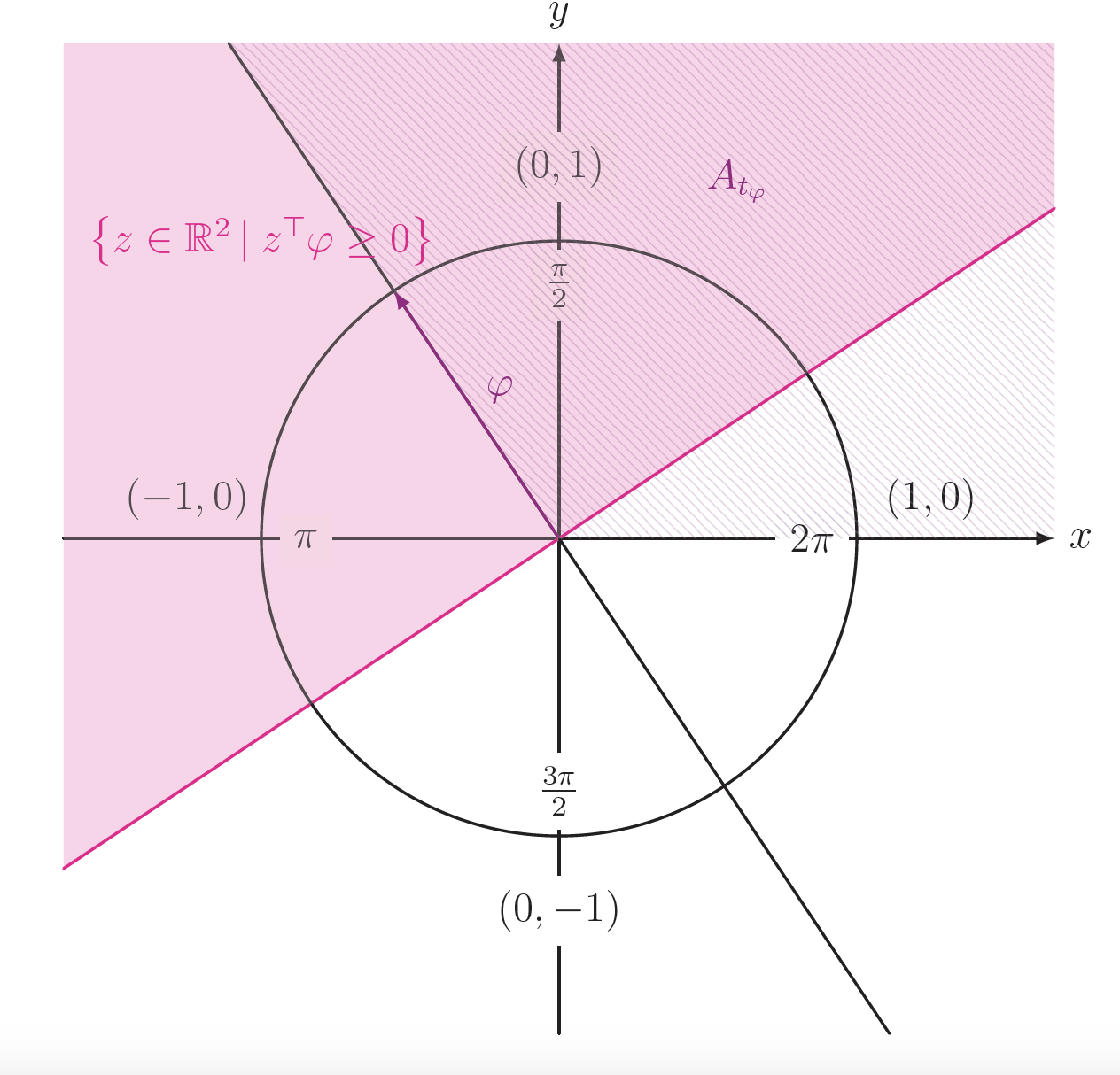
Figure 3: The half space $\left\{z\in\mathbb{R}^{2}\left|\right.z^{\top}\varphi\geq 0\right\}$ for $\varphi$ and the corresponding circular sector $A_{t_{\varphi}}$. It follows that $\left\{z\in\mathbb{R}^{2}\left|\right.z^{\top}\varphi\geq 0\right\}=A_{t_{\varphi}+\frac{\pi}{2}}\setminus A_{t_{\varphi}-\frac{\pi}{2}}\cup\left\{z\in\mathbb{R}^{2}\left|\right.z_{1}\geq 0,z_{2}\geq 0,z^{\top}\varphi=0\right\}$.

It then follows that

$$\left\{z\in\mathbb{R}^{2}\left|\right.(z-x)^{\top}\varphi\geq 0\right\}$$

$$= (\{x+A_{t_{\varphi}+\frac{\pi}{2}}\}\setminus\{x+A_{t_{\varphi}-\frac{\pi}{2}}\})\cup\left\{z\in\mathbb{R}^{2}\left|\right.z_{1}-x_{1}\geq 0,z_{2}-x_{2}\geq 0,z^{\top}\varphi=0\right\},$$

where the two sets are disjoint and $\{x+A_{t_{\varphi}-\frac{\pi}{2}}\}\subset\{x+A_{t_{\varphi}+\frac{\pi}{2}}\}$. As a result, we have

$$Q^{(n)}\left(\left\{z\in\mathbb{R}^{2}\left|\right.(z-x)^{\top}\varphi\geq 0\right\}\right)$$ (4)

$$= Q^{(n)}\left(\{x+A_{t_{\varphi}+\frac{\pi}{2}}\}\setminus\{x+A_{t_{\varphi}-\frac{\pi}{2}}\}\right)$$

$$+Q^{(n)}\left(\left\{z\in\mathbb{R}^{2}\setminus\{x\}\left|\right.z_{1}-x_{1}\geq 0,z_{2}-x_{2}\geq 0,(z-x)^{\top}\varphi=0\right\}\right)$$

$$= Q^{(n)}\left(x+A_{t_{\varphi}+\frac{\pi}{2}}\right)-Q^{(n)}\left(x+A_{t_{\varphi}-\frac{\pi}{2}}\right)$$

$$+Q^{(n)}\left(\left\{z\in\mathbb{R}^{2}\left|\right.z_{1}-x_{1}\geq 0,z_{2}-x_{2}\geq 0,(z-x)^{\top}\varphi=0\right\}\right).$$

The third term converges uniformly in $\varphi$ due to Lemma 5.1. Analyzing the convergence of the first two summands reduces to studying

$$F_{Q^{(n)}_{\Pi_{x}}}(t)=Q^{(n)}\left(\Pi_{x}^{-1}\left[0,t\right]\right)=Q^{(n)}(x+A_{t})$$

for $t\in(0,2\pi]$. The left-hand side of the above formula corresponds to a distribution function converging uniformly to the continuous limit function $F_{Q_{\Pi_{x}}}(t)$.

Now, let $\varphi_{1}>0$ (case 2). Then, we have

$$a_{n}(\varphi)= Q^{(n)}\left(\left\{z\in\mathbb{R}^{d}|(z-x)^{T}\varphi\geq 0\right\}\right)=1-Q^{(n)}\left(\left\{z\in\mathbb{R}^{d}|(z-x)^{T}\varphi<0\right\}\right)$$

$$= 1-Q^{(n)}\left(\left\{z\in\mathbb{R}^{d}|(z-x)^{T}(-\varphi)>0\right\}\right)$$

$$= 1-Q^{(n)}\left(\left\{z\in\mathbb{R}^{d}|(z-x)^{T}(-\varphi)\geq 0\right\}\right)$$

$$+Q^{(n)}\left(\left\{z\in\mathbb{R}^{d}|(z-x)^{T}(-\varphi)=0\right\}\right)$$

$$= 1-a_{n}(-\varphi)+Q^{(n)}\left(\left\{z\in\mathbb{R}^{d}|(z-x)^{T}(-\varphi)=0\right\}\right).$$

The last summand on the right-hand side of the above equation converges uniformly in $\varphi$ due to Lemma 5.1.

Finally, let $\varphi_{1}=0$ (case 3). In this case, we have only two points on the sphere and hence uniform convergence on these points follows immediately. Putting all results together, we obtain:

$$\sup_{\varphi\in S^{2}}\left|a_{n}(\varphi)-a(\varphi)\right|\longrightarrow 0$$

and consequently

$$D_{Q_{Y_{n}}}(x)=\inf_{\varphi\in S^{2}}a_{n}(\varphi)\longrightarrow\inf_{\varphi\in S^{2}}a(\varphi)=D_{Q_{Y}}(x).$$

∎

5 Appendix

Here we present the lemmas which are used in order to proof Proposition 4.2. Lines, respectively half lines, play an important role. The following lemma allows to handle them in the context of uniform convergence.

Lemma 5.1.

Let $Q^{(n)}$, $Q$ and $\Pi_{x}$ be as above. $\varphi_{1}\leq 0$. Then

$$Q^{(n)}\left(\left\{z\in\mathbb{R}^{2}\left|\right.(z-x)^{\top}\varphi=0,z_{2}-x_{2}>0\right\}\right)$$

$$\longrightarrow Q\left(\left\{z\in\mathbb{R}^{2}\left|\right.(z-x)^{\top}\varphi=0,z_{2}-x_{2}>0\right\}\right)$$

and

$$Q^{(n)}\left(\left\{z\in\mathbb{R}^{2}\left|\right.(z-x)^{\top}\varphi=0\right\}\right)\longrightarrow Q\left(\left\{z\in\mathbb{R}^{2}\left|\right.(z-x)^{\top}\varphi=0\right\}\right)$$

uniformly in $\varphi$.

Proof.

Knowing that the distribution function $F_{Q^{(n)}_{\Pi_{x}}}(t)$ converges pointwise towards a continuous limit, we conclude that it converges uniformly. From this fact, we can also derive that the jumps

$$F_{Q^{(n)}_{\Pi_{x}}}(t)-F_{Q^{(n)}_{\Pi_{x}}}(t-)=Q^{(n)}_{\Pi_{x}}(\{t\})$$

converge uniformly in $t$. Hence,

$$Q^{(n)}\left(\left\{z\in\mathbb{R}^{2}\left|\right.(z-x)^{\top}\varphi=0,z_{2}-x_{2}>0\right\}\right)=Q^{(n)}_{\Pi_{x}}(\{t_{\varphi}-\frac{\pi}{2}\})$$

converges uniformly in $\varphi$. Analogously, this holds for $z_{2}-x_{2}<0$. For $z_{2}-x_{2}=0$ we only obtain a single point, and hence, no dependence on $\varphi$. This yields uniform convergence of the sum of the three functions

$$\varphi\mapsto Q^{(n)}\left(\left\{z\in\mathbb{R}^{2}\left|\right.(z-x)^{\top}\varphi=0\right\}\right)$$

which is the measure of the full line. ∎

Definition 5.2.

Let $(\Omega,\mathcal{F},P,T)$ be a measure preserving dynamical system. A measurable set $A\subset\Omega$ is called $T$-invariant if $T^{-1}A=A$. Then

$$\mathcal{I}:=\left\{A:T^{-1}(A)=A\right\}$$

denotes the $\sigma$-field of invariant sets. $T$ is called ergodic if $\mathcal{I}$ is trivial, i.e. $P(A)\in\{0,1\}$ for all $A\in\mathcal{I}$. A stationary stochastic process $(X_{t})_{t\in\mathbb{N}}$ with values in $S$ is called ergodic if the shift on $(S^{\mathbb{N}},\mathcal{S}^{\mathbb{N}},P_{X})$ is ergodic.

Lemma 5.3.

Suppose that $(X_{j})_{j\in\mathbb{N}}$ is a stationary ergodic process with state space $S$ and $f:S^{\mathbb{N}}\longrightarrow\mathbb{R}$ a measurable function. Then $(Y_{j})_{j\in\mathbb{N}}$ with $Y_{i}=f(X_{i},X_{i+1},\ldots)$ is stationary ergodic as well.

Proof.

It is a well-known fact that measurable transformations preserve strict stationarity. Therefore, it suffices to prove ergodicity of $(Y_{j})_{j\in\mathbb{N}}$. For this, let $T$ denote the shift operator and let $A\in\mathcal{I}_{Y}$, i.e.

$$y=(y_{0},y_{1},\ldots)\in A\Leftrightarrow(y_{1},y_{2},\ldots)\in A.$$

Define

$$B:=\{x:(f(x_{0},x_{1},\ldots),f(x_{1},x_{2},\ldots),\ldots)\in A\}.$$

Then, it holds that $P_{X}(B)=P(X\in B)=P(Y\in A)=P_{Y}(A)$. Moreover, $B$ is shift invariant as well since

$$x\in B \Leftrightarrow(f(x_{0},x_{1},\ldots),f(x_{1},x_{2},\ldots),\ldots)\in A$$

$$\Leftrightarrow(f(x_{1},x_{2},\ldots),f(x_{2},x_{3},\ldots),\ldots)\in A$$

$$\Leftrightarrow(x_{1},x_{2},\ldots)=T(x)\in B.$$

As a result, since $P_{X}(B)\in\{0,1\}$ for all $B\in\mathcal{I}_{X}$, $f$ is ergodic. ∎

Lemma 5.4.

Let $\varphi=(\varphi_{1},\varphi_{2})\in S^{2}$ with $\varphi_{1}<0$. For $t_{\varphi}:=\arctan\left(\frac{\varphi_{2}}{\varphi_{1}}\right)+\pi$ it holds that

$$\left\{z\in\mathbb{R}^{2}\left|\right.z^{\top}\varphi\geq 0\right\}$$

$$= A_{t_{\varphi}+\frac{\pi}{2}}\setminus A_{t_{\varphi}-\frac{\pi}{2}}\cup\left\{z\in\mathbb{R}^{2}\left|\right.z_{1}\geq 0,z_{2}\geq 0,z^{\top}\varphi=0\right\},$$

where for $t\in[0,2\pi)$ the subset $A_{t}$ of $\mathbb{R}^{2}$ is defined by

$$A_{t}:=W^{-1}\left(\pi_{2}^{-1}\left[0,t\right]\right).$$

Proof.

Consider $\varphi=(\varphi_{1},\varphi_{2})\in S^{2}$ with $\varphi_{1}<0$ and $\varphi_{2}>0$. Then, for $t_{\varphi}=\pi_{2}\circ W(\varphi)=\arctan\left(\frac{\varphi_{2}}{\varphi_{1}}\right)+\pi$, it follows that

$$A_{t_{\varphi}+\frac{\pi}{2}}= W^{-1}\left(\pi_{2}^{-1}\left[0,t_{\varphi}+\frac{\pi}{2}\right]\right)=W^{-1}\left((0,\infty)\times\left[0,t_{\varphi}+\frac{\pi}{2}\right]\right)$$

$$= \left\{z\in\mathbb{R}^{2}\setminus\{(0,0)\}\left|\right.W(z)\in(0,\infty)\times\left[0,t_{\varphi}+\frac{\pi}{2}\right]\right\}$$

$$= \left\{z\in\mathbb{R}^{2}\setminus\{(0,0)\}\left|\right.W(z)\in(0,\infty)\times\left[0,\frac{\pi}{2}\right)\right\}$$

$$\cup\left\{z\in\mathbb{R}^{2}\setminus\{(0,0)\}\left|\right.W(z)\in(0,\infty)\times\frac{\pi}{2}\right\}$$

$$\cup\left\{z\in\mathbb{R}^{2}\setminus\{(0,0)\}\left|\right.W(z)\in(0,\infty)\times\left(\frac{\pi}{2},t_{\varphi}+\frac{\pi}{2}\right]\right\}$$

$$= \left\{z\in\mathbb{R}^{2}\setminus\{(0,0)\}\left|\right.z_{1}>0,z_{2}\geq 0\right\}$$

$$\cup\left\{z\in\mathbb{R}^{2}\setminus\{(0,0)\}\left|\right.z_{1}=0,z_{2}>0\right\}$$

$$\cup\left\{z\in\mathbb{R}^{2}\setminus\{(0,0)\}\left|\right.z_{1}<0,\arctan\left(\frac{z_{2}}{z_{1}}\right)+\pi\leq\arctan\left(\frac{\varphi_{2}}{\varphi_{1}}\right)+\frac{3\pi}{2}\right\}.$$

Since $\tan\left(x+\frac{\pi}{2}\right)=-\frac{1}{\tan(x)}$, the third set can be written as follows:

$$\left\{z\in\mathbb{R}^{2}\setminus\{(0,0)\}\left|\right.z_{1}<0,\arctan\left(\frac{z_{2}}{z_{1}}\right)+\pi\leq\arctan\left(\frac{\varphi_{2}}{\varphi_{1}}\right)+\frac{3\pi}{2}\right\}$$

$$= \left\{z\in\mathbb{R}^{2}\setminus\{(0,0)\}\left|\right.z_{1}<0,\arctan\left(\frac{z_{2}}{z_{1}}\right)\leq\arctan\left(\frac{\varphi_{2}}{\varphi_{1}}\right)+\frac{\pi}{2}\right\}$$

$$= \left\{z\in\mathbb{R}^{2}\setminus\{(0,0)\}\left|\right.z_{1}<0,\frac{z_{2}}{z_{1}}\leq-\frac{\varphi_{1}}{\varphi_{2}}\right\}$$

$$= \left\{z\in\mathbb{R}^{2}\setminus\{(0,0)\}\left|\right.z_{1}<0,z_{1}\varphi_{1}+z_{2}\varphi_{2}\geq 0\right\}$$

$$= \left\{z\in\mathbb{R}^{2}\setminus\{(0,0)\}\left|\right.z_{1}<0,z^{\top}\varphi\geq 0\right\}.$$

Moreover, we have

$$A_{t_{\varphi}-\frac{\pi}{2}}= W^{-1}\left(\pi_{2}^{-1}\left[0,t_{\varphi}-\frac{\pi}{2}\right]\right)=W^{-1}\left((0,\infty)\times\left[0,t_{\varphi}-\frac{\pi}{2}\right]\right)$$

$$= \left\{z\in\mathbb{R}^{2}\setminus\{(0,0)\}\left|\right.W(z)\in(0,\infty)\times\left[0,t_{\varphi}-\frac{\pi}{2}\right]\right\}$$

$$= \left\{z\in\mathbb{R}^{2}\setminus\{(0,0)\}\left|\right.z_{1}>0,z_{2}\geq 0,\arctan\left(\frac{z_{2}}{z_{1}}\right)\leq t_{\varphi}-\frac{\pi}{2}\right\}$$

$$= \left\{z\in\mathbb{R}^{2}\setminus\{(0,0)\}\left|\right.z_{1}>0,z_{2}\geq 0,\arctan\left(\frac{z_{2}}{z_{1}}\right)\leq\arctan\left(\frac{\varphi_{2}}{\varphi_{1}}\right)+\frac{\pi}{2}\right\}$$

$$= \left\{z\in\mathbb{R}^{2}\setminus\{(0,0)\}\left|\right.z_{1}>0,z_{2}\geq 0,\frac{z_{2}}{z_{1}}\leq-\frac{\varphi_{1}}{\varphi_{2}}\right\}$$

$$= \left\{z\in\mathbb{R}^{2}\setminus\{(0,0)\}\left|\right.z_{1}>0,z_{2}\geq 0,z_{1}\varphi_{1}+z_{2}\varphi_{2}\leq 0\right\}$$

$$= \left\{z\in\mathbb{R}^{2}\setminus\{(0,0)\}\left|\right.z_{1}>0,z_{2}\geq 0,z^{\top}\varphi\leq 0\right\}.$$

As a result, it holds that

$$A_{t_{\varphi}+\frac{\pi}{2}}\setminus A_{t_{\varphi}-\frac{\pi}{2}}= \left\{z\in\mathbb{R}^{2}\setminus\{(0,0)\}\left|\right.z_{1}>0,z_{2}\geq 0,z^{\top}\varphi>0\right\}$$

$$\cup\left\{z\in\mathbb{R}^{2}\setminus\{(0,0)\}\left|\right.z_{1}=0,z_{2}>0\right\}$$

$$\cup\left\{z\in\mathbb{R}^{2}\setminus\{(0,0)\}\left|\right.z_{1}<0,z^{\top}\varphi\geq 0\right\}.$$

Therefore, we have

$$\left\{z\in\mathbb{R}^{2}\left|\right.(z-x)^{\top}\varphi\geq 0\right\}$$

$$= \{A_{t_{\varphi}+\frac{\pi}{2}}+x\}\setminus\{A_{t_{\varphi}-\frac{\pi}{2}}+x\}\cup\left\{z\in\mathbb{R}^{2}\left|\right.z_{1}-x_{1}\geq 0,z_{2}-x_{2}\geq 0,(z-x)^{\top}\varphi=0\right\}.$$

Consider $\varphi=(\varphi_{1},\varphi_{2})\in S^{2}$ with $\varphi_{1}<0$ and $\varphi_{2}<0$. Then, for $t_{\varphi}=\pi_{2}\circ W(\varphi)=\arctan\left(\frac{\varphi_{2}}{\varphi_{1}}\right)+\pi$ it follows that

$$A_{t_{\varphi}+\frac{\pi}{2}}= W^{-1}\left(\pi_{2}^{-1}\left[0,t_{\varphi}+\frac{\pi}{2}\right]\right)=W^{-1}\left((0,\infty)\times\left[0,t_{\varphi}+\frac{\pi}{2}\right]\right)$$

$$= \left\{z\in\mathbb{R}^{2}\setminus\{(0,0)\}\left|\right.W(z)\in(0,\infty)\times\left[0,t_{\varphi}+\frac{\pi}{2}\right]\right\}$$

$$= \left\{z\in\mathbb{R}^{2}\setminus\{(0,0)\}\left|\right.W(z)\in(0,\infty)\times\left[0,\frac{\pi}{2}\right)\right\}$$

$$\cup\left\{z\in\mathbb{R}^{2}\setminus\{(0,0)\}\left|\right.W(z)\in(0,\infty)\times\frac{\pi}{2}\right\}$$

$$\cup\left\{z\in\mathbb{R}^{2}\setminus\{(0,0)\}\left|\right.W(z)\in(0,\infty)\times\left(\frac{\pi}{2},\frac{3\pi}{2}\right)\right\}$$

$$\cup\left\{z\in\mathbb{R}^{2}\setminus\{(0,0)\}\left|\right.W(z)\in(0,\infty)\times\frac{3\pi}{2}\right\}$$

$$\cup\left\{z\in\mathbb{R}^{2}\setminus\{(0,0)\}\left|\right.W(z)\in(0,\infty)\times\left(\frac{3\pi}{2},t_{\varphi}+\frac{\pi}{2}\right]\right\}$$

$$= \left\{z\in\mathbb{R}^{2}\setminus\{(0,0)\}\left|\right.z_{1}>0,z_{2}\geq 0\right\}$$

$$\cup\left\{z\in\mathbb{R}^{2}\setminus\{(0,0)\}\left|\right.z_{1}=0,z_{2}>0\right\}$$

$$\cup\left\{z\in\mathbb{R}^{2}\setminus\{(0,0)\}\left|\right.z_{1}<0\right\}$$

$$\cup\left\{z\in\mathbb{R}^{2}\setminus\{(0,0)\}\left|\right.z_{1}=0,z_{2}<0\right\}$$

$$\cup\left\{z\in\mathbb{R}^{2}\setminus\{(0,0)\}\left|\right.z_{1}>0,z_{2}<0,\arctan\left(\frac{z_{2}}{z_{1}}\right)+2\pi\leq t_{\varphi}+\frac{\pi}{2}\right\}.$$

Since $\tan\left(x-\frac{\pi}{2}\right)=-\frac{1}{\tan(x)}$, the fifth set can be written as follows:

$$\left\{z\in\mathbb{R}^{2}\setminus\{(0,0)\}\left|\right.z_{1}>0,z_{2}<0,\arctan\left(\frac{z_{2}}{z_{1}}\right)+2\pi\leq t_{\varphi}+\frac{\pi}{2}\right\}$$

$$=\left\{z\in\mathbb{R}^{2}\setminus\{(0,0)\}\left|\right.z_{1}>0,z_{2}<0,\arctan\left(\frac{z_{2}}{z_{1}}\right)\leq\arctan\left(\frac{\varphi_{2}}{\varphi_{1}}\right)-\frac{\pi}{2}\right\}$$

$$=\left\{z\in\mathbb{R}^{2}\setminus\{(0,0)\}\left|\right.z_{1}>0,z_{2}<0,\frac{z_{2}}{z_{1}}\leq-\frac{\varphi_{1}}{\varphi_{2}}\right\}$$

$$=\left\{z\in\mathbb{R}^{2}\setminus\{(0,0)\}\left|\right.z_{1}>0,z_{2}<0,z_{2}\varphi_{2}+z_{1}\varphi_{1}\geq 0\right\}$$

$$=\left\{z\in\mathbb{R}^{2}\setminus\{(0,0)\}\left|\right.z_{1}>0,z_{2}<0,z^{\top}\varphi\geq 0\right\}.$$

Moreover, we have

$$A_{t_{\varphi}-\frac{\pi}{2}}= W^{-1}\left(\pi_{2}^{-1}\left[0,t_{\varphi}-\frac{\pi}{2}\right]\right)$$

$$= W^{-1}\left((0,\infty)\times\left[0,\frac{\pi}{2}\right)\right)$$

$$\cup W^{-1}\left((0,\infty)\times\frac{\pi}{2}\right)$$

$$\cup W^{-1}\left((0,\infty)\times\left(\frac{\pi}{2},t_{\varphi}-\frac{\pi}{2}\right]\right)$$

$$= \left\{z\in\mathbb{R}^{2}\setminus\{(0,0)\}\left|\right.z_{1}>0,z_{2}\geq 0\right\}$$

$$\cup\left\{z\in\mathbb{R}^{2}\setminus\{(0,0)\}\left|\right.z_{1}=0,z_{2}>0\right\}$$

$$\cup\left\{z\in\mathbb{R}^{2}\setminus\{(0,0)\}\left|\right.z_{1}<0,\arctan\left(\frac{z_{2}}{z_{1}}\right)+\pi\leq\arctan\left(\frac{\varphi_{2}}{\varphi_{1}}\right)+\frac{\pi}{2}\right\}.$$

Since $\tan\left(x-\frac{\pi}{2}\right)=-\frac{1}{\tan(x)}$, the third set can be written as follows:

$$\left\{z\in\mathbb{R}^{2}\setminus\{(0,0)\}\left|\right.z_{1}<0,\arctan\left(\frac{z_{2}}{z_{1}}\right)+\pi\leq\arctan\left(\frac{\varphi_{2}}{\varphi_{1}}\right)+\frac{\pi}{2}\right\}$$

$$=\left\{z\in\mathbb{R}^{2}\setminus\{(0,0)\}\left|\right.z_{1}<0,\arctan\left(\frac{z_{2}}{z_{1}}\right)\leq\arctan\left(\frac{\varphi_{2}}{\varphi_{1}}\right)-\frac{\pi}{2}\right\}$$

$$=\left\{z\in\mathbb{R}^{2}\setminus\{(0,0)\}\left|\right.z_{1}<0,\frac{z_{2}}{z_{1}}\leq-\frac{\varphi_{1}}{\varphi_{2}}\right\}$$

$$=\left\{z\in\mathbb{R}^{2}\setminus\{(0,0)\}\left|\right.z_{1}<0,z^{\top}\varphi\leq 0\right\}.$$

So far, we covered the cases $\varphi_{1}<0$, $\varphi_{2}>0$ and $\varphi_{1}<0$, $\varphi_{2}<0$. For $\varphi_{1}<0$ and $\varphi_{2}=0$, we have $t_{\varphi}=\pi$. It follows that

$$A_{t_{\varphi}+\frac{\pi}{2}}= W^{-1}\left(\pi_{2}^{-1}\left[0,\frac{3\pi}{2}\right]\right)=W^{-1}\left((0,\infty)\times\left[0,\frac{3\pi}{2}\right]\right)$$

$$= \left\{z\in\mathbb{R}^{2}\setminus\{(0,0)\}\left|\right.z_{1}>0,z_{2}\geq 0\right\}$$

$$\cup\left\{z\in\mathbb{R}^{2}\setminus\{(0,0)\}\left|\right.z_{1}=0,z_{2}>0\right\}$$

$$\cup\left\{z\in\mathbb{R}^{2}\setminus\{(0,0)\}\left|\right.z_{1}<0\right\}$$

$$\cup\left\{z\in\mathbb{R}^{2}\setminus\{(0,0)\}\left|\right.z_{1}=0,z_{2}<0\right\}.$$

Moreover, we have

$$A_{t_{\varphi}-\frac{\pi}{2}}= W^{-1}\left(\pi_{2}^{-1}\left[0,\frac{\pi}{2}\right]\right)$$

$$= \left\{z\in\mathbb{R}^{2}\setminus\{(0,0)\}\left|\right.z_{1}>0,z_{2}\geq 0\right\}$$

$$\cup\left\{z\in\mathbb{R}^{2}\setminus\{(0,0)\}\left|\right.z_{1}=0,z_{2}>0\right\}.$$

As a result, it holds that

$$A_{t_{\varphi}+\frac{\pi}{2}}\setminus A_{t_{\varphi}-\frac{\pi}{2}}= \left\{z\in\mathbb{R}^{2}\setminus\{(0,0)\}\left|\right.z_{1}<0\right\}$$

$$\cup\left\{z\in\mathbb{R}^{2}\setminus\{(0,0)\}\left|\right.z_{1}=0,z_{2}<0\right\}.$$

Therefore, we have

$$\left\{z\in\mathbb{R}^{2}\left|\right.(z-x)^{\top}\varphi\geq 0\right\}$$

$$= \left\{z\in\mathbb{R}^{2}\left|\right.z_{1}-x_{1}\leq 0\right\}$$

$$= \{A_{t_{\varphi}+\frac{\pi}{2}}+x\}\setminus\{A_{t_{\varphi}-\frac{\pi}{2}}+x\}$$

$$\cup\left\{z\in\mathbb{R}^{2}\left|\right.z_{1}-x_{1}\geq 0,z_{2}-x_{2}\geq 0,(z-x)^{\top}\varphi=0\right\}.$$

∎

References

• Bandt (2005) Christoph Bandt. Ordinal time series analysis. Ecological modelling, 182(3-4):229–238, 2005.
• Bandt and Pompe (2002) Christoph Bandt and Bernd Pompe. Permutation Entropy: A Natural Complexity Measure for Time Series. Physical review letters, 88(17):174102–1 – 174102–4, 2002.
• Barnett (1976) Vic Barnett. The ordering of multivariate data. Journal of the Royal Statistical Society: Series A (General), 139(3):318–344, 1976.
• Betken et al. (2021a) Annika Betken, Jannis Buchsteiner, Herold Dehling, Ines Münker, Alexander Schnurr, and Jeannette H.C. Woerner. Ordinal patterns in long-range dependent time series. Scandinavian Journal of Statistics, 48(3):969 – 1000, 2021a.
• Betken et al. (2021b) Annika Betken, Herold Dehling, Ines Nüßgen, and Alexander Schnurr. Ordinal pattern dependence as a multivariate dependence measure. Journal of Multivariate Analysis, 186(C):104798, 2021b.
• Chernozhukov et al. (2017) Victor Chernozhukov, Alfred Galichon, Marc Hallin, and Marc Henry. Monge–Kantorovich depth, quantiles, ranks and signs. The Annals of Statistics, 45(1):223–256, 2017.
• Cornfeld et al. (2012) Isaac P. Cornfeld, Sergei Vasilevich Fomin, and Yakov Grigor’evǐc Sinai. Ergodic theory, volume 245. Springer Science & Business Media, 2012.
• Cuesta-Albertos and Nieto-Reyes (2008) Juan Antonio Cuesta-Albertos and Alicia Nieto-Reyes. The random Tukey depth. Computational Statistics & Data Analysis, 52(11):4979–4988, 2008.
• Donoho and Gasko (1992) David L. Donoho and Miriam Gasko. Breakdown properties of location estimates based on halfspace depth and projected outlyingness. The Annals of Statistics, 20(3):1803–1827, 1992.
• Ghosh and Chaudhuri (2005) Anil K. Ghosh and Probal Chaudhuri. On maximum depth and related classifiers. Scandinavian Journal of Statistics, 32(2):327–350, 2005.
• Hassairi and Regaieg (2008) Abdelhamid Hassairi and Ons Regaieg. On the Tukey depth of a continuous probability distribution. Statistics & probability letters, 78(15):2308–2313, 2008.
• He et al. (2016) Shaobo He, Kehui Sun, and Huihai Wang. Multivariate permutation entropy and its application for complexity analysis of chaotic systems. Physica A: Statistical Mechanics and its Applications, 461:812–823, 2016.
• Ibragimov and Linnik (1971) I. A. Ibragimov and Yu V. Linnik. Independent and stationary sequences of random variables. Wolters, Noordhoff Pub., 1971.
• Keller and Lauffer (2003) Karsten Keller and Heinz Lauffer. Symbolic analysis of high-dimensional time series. International Journal of Bifurcation and Chaos, 13(09):2657–2668, 2003.
• Keller et al. (2015) Karsten Keller, Sergiy Maksymenko, and Inga Stolz. Entropy determination based on the ordinal structure of a dynamical system. Discrete and Continuous Dynamical Systems - B, 20(10):3507–3524, 2015.
• Koshevoy (2002) Gleb A Koshevoy. The tukey depth characterizes the atomic measure. Journal of Multivariate Analysis, 83(2):360–364, 2002.
• Liu (1990) Regina Y. Liu. On a notion of data depth based on random simplices. The Annals of Statistics, 18(1):405–414, 1990.
• Mahalanobis (1936) Prasanta Chandra Mahalanobis. On the generalized distance in statistics. National Institute of Science of India, 1936.
• Mohr et al. (2020) Marisa Mohr, Florian Wilhelm, Mattis Hartwig, Ralf Möller, and Karsten Keller. New approaches in ordinal pattern representations for multivariate time series. In FLAIRS Conference, pages 124–129, 2020.
• Mosler (2002) Karl Mosler. Multivariate dispersion, central regions, and depth: the lift zonoid approach, volume 165. Springer Science & Business Media, 2002.
• Oja (1983) Hannu Oja. Descriptive statistics for multivariate distributions. Statistics & Probability Letters, 1(6):327–332, 1983.
• Rayan et al. (2019) Yomna Rayan, Yasser Mohammad, and Samia A Ali. Multidimensional permutation entropy for constrained motif discovery. In Intelligent Information and Database Systems: 11th Asian Conference, ACIIDS 2019, Yogyakarta, Indonesia, April 8–11, 2019, Proceedings, Part I 11, pages 231–243. Springer, 2019.
• Schnurr (2014) Alexander Schnurr. An ordinal pattern approach to detect and to model leverage effects and dependence structures between financial time series. Statistical Papers, 55(4):919 – 931, 2014.
• Schnurr and Dehling (2017) Alexander Schnurr and Herold Dehling. Testing for Structural Breaks via Ordinal Pattern Dependence. Journal of the American Statistical Association, 112(518):706 – 720, 2017.
• Schnurr and Fischer (2022) Alexander Schnurr and Svenja Fischer. Generalized ordinal patterns allowing for ties and their applications in hydrology. Computational Statistics & Data Analysis, 171:107472, 2022.
• Sinn et al. (2012) Mathieu Sinn, Ali Ghodsi, and Karsten Keller. Detecting Change-Points in Time Series by Maximum Mean Discrepancy of Ordinal Pattern Distributions. UAI’12 Proceedings of the Twenty-Eighth Conference on Uncertainty in Artificial Intelligence, pages 786 – 794, 2012.
• Zuo and Serfling (2000a) Yijun Zuo and Robert Serfling. General notions of statistical depth function. Annals of Statistics, 28(2):461–482, 2000a.
• Zuo and Serfling (2000b) Yijun Zuo and Robert Serfling. Structural properties and convergence results for contours of sample statistical depth functions. Annals of Statistics, 28(2):483–499, 2000b.