Flaring Stars in a Non-targeted mm-wave Survey with SPT-3G

Abstract

We present a flare star catalog from four years of non-targeted millimeter-wave survey data from the South Pole Telescope (SPT). The data were taken with the SPT-3G camera and cover a 1500-square-degree region of the sky from 20^h40^m0^s to 3^h20^m0^s in right ascension and $-42\text{\,}\mathrm{\SIUnitSymbolDegree}$ to $-70\text{\,}\mathrm{\SIUnitSymbolDegree}$ in declination. This region was observed on a nearly daily cadence from 2019-2022 and chosen to avoid the plane of the galaxy. A short-duration transient search of this survey yields 111 flaring events from 66 stars, increasing the number of both flaring events and detected flare stars by an order of magnitude from the previous SPT-3G data release. We provide cross-matching to Gaia DR3, as well as matches to X-ray point sources found in the second ROSAT all-sky survey. We have detected flaring stars across the main sequence, from early-type A stars to M dwarfs, as well as a large population of evolved stars. These stars are mostly nearby, spanning 10 to 1000 parsecs in distance. Most of the flare spectral indices are constant or gently rising as a function of frequency at 95/150/220 GHz. The timescale of these events can range from minutes to hours, and the peak $\nu L_{\nu}$ luminosities range from $10^{27}$ to $10^{31}$ erg s^-1 in the SPT-3G frequency bands.

tablenum SIXtablenum

1 Introduction

Flaring activity in stars can be found across a wide range of spectral types (Balona, 2015) and is thought to result from a release of magnetic energy. The Sun is also known to flare, and has been extensively studied from radio wavelengths to gamma-rays (Fletcher et al., 2011; Benz, 2017) including the millimeter wavelengths (Silva et al., 1996) studied in this paper. Solar flares have been used to serve as a framework for our understanding of flaring activities on other stars (Pettersen, 1989). While there are similarities in processes and the physics between many solar and stellar flares (Aschwanden et al., 2008), the utility of these comparisons reaches a limit as the Sun is atypical when looking at larger stellar populations. For example, even when considering other “Sun-like” stars (stars with similarities such as spectral type, age, rotation period, and position along the main sequence), the Sun has been shown to exhibit substantially lower photometric variability (Reinhold et al., 2020). Typical solar flares have optical energies of $\sim 10^{29}$ erg with a maximum of $\sim 10^{31}$ erg in X-ray. On the extreme side, flares as strong as $\sim 10^{38}$ erg at optical wavelengths have been observed on “Sun-like” stars (Schaefer et al., 2000).

The generally accepted model of stellar flares (Brown, 1971; Hudson, 1972) involves a sudden release of energy triggered by reconnection of magnetic field lines, resulting in acceleration of charged particles that emit radiation across the electromagnetic spectrum (Allred et al., 2015; Benz, 2017). Different wavelengths track different physics of the flare: charged particles are accelerated from this area of reconnection in an impulsive event, seen simultaneously as gyrosynchrotron in radio wavelengths and bremsstrahlung in hard X-rays (HXR, $\gtrsim 10$ keV) (Bastian et al., 1998; Massi et al., 2002; Benz & Güdel, 2010). The particles travel along the field lines, eventually depositing their energy lower in the stellar atmosphere. This energy heats and evaporates plasma back into the upper atmosphere and can be seen in optical/ultraviolet (UV) (Krucker et al., 2015; Henry & Newsom, 1996). As this plasma reaches the corona, the emission transitions from a sudden and fast rise in energy released to a gradual rise that can be seen in soft X-ray (SXR, $\lesssim 10$ keV) as cooling starts (Güdel, 2004).

External interactions between stars can also produce flaring events. RS Canum Venaticorum variable stars (RS CVn) and other binary systems have shown flares across the electromagnetic spectrum which can be due to interactions in the magnetic field shared between components of the system (Catalano, 1986; Massi et al., 2002). Protostars and young, pre-main sequence stars (e.g. T Tauri) that still have an accretion disk can exhibit flares due to magnetic field interactions between the star and the disk itself (Feigelson & Montmerle, 1999).

At radio wavelengths, solar flares typically show a peak at 1-10 GHz which is thought to correspond to mildly relativistic synchrotron radiation as the source transitions from from optically thick to optically thin, with the optically thin part of the spectrum extending into millimeter wavelengths (Bastian et al., 1998). Peak flux spectra of solar flares show flux at 5 GHz to be over an order of magnitude larger than flux at 30 GHz (Kundu & Vlahos, 1982), with more recent observations exhibiting a similar falling spectrum between flux at 3.4-17 GHz and 86 GHz (Raulin et al., 1999) and even out to 345 GHz (Lüthi et al., 2004). Rising spectra at submillimeter wavelengths have been occasionally observed in solar flares (Zhou et al., 2011), with radiative processes such as bremsstrahlung and gyrosynchrotron requiring extreme parameters as possible explanations (Krucker et al., 2013).

Stellar flare astronomy has historically involved targeted observations of individual stars (e.g. Large et al., 1989; Webber et al., 1973). Recent years have seen massive growth in the field of time-domain astronomy with exoplanet detecting experiments Kepler (Koch et al., 2010), and TESS (Ricker et al., 2014) providing an observing cadence as high as 2 minutes, or even 20 seconds for a small number of bright candidates. This high cadence data is invaluable for monitoring the variability of stars, and has resulted in enormous catalogs of stellar flares at optical wavelengths (Davenport, 2016; Günther et al., 2020). Transient surveys have also been carried out at infrared (Davenport et al., 2012), UV (Brasseur et al., 2019; Loyd et al., 2018a), and X-ray (Pye et al., 2015; Getman & Feigelson, 2021).

At longer wavelengths, radio observations of stellar flares have been mainly composed of targeted observations (Loyd et al., 2018b; Smith et al., 2005) and recent archival surveys (Levinson et al., 2002). In the future, radio wavelength surveys such as SKA pathfinders, and eventually SKA, will monitor the southern sky for radio transients (Murphy et al., 2013).

While observations of stellar flares at or near millimeter wavelengths have been made in the past (Burton et al., 2022; MacGregor et al., 2021, 2020, 2018; Massi et al., 2006; Umemoto et al., 2009; Brown & Brown, 2006; Beasley & Bastian, 1998; Mairs et al., 2019), there have not been any dedicated transient surveys at these wavelengths until those conducted with the South Pole Telescope (SPT Guns et al., 2021; Whitehorn et al., 2016) which yielded 13 stellar flares from 8 stars, and the Atacama Cosmology Telescope (ACT Li et al., 2023; Naess et al., 2021) which yielded a total of 17 stellar flares from 14 stars.

Stellar flares detected by SPT and the ACT have been in the range of $\nu L_{\nu}\sim 10^{26}-10^{30}$ erg s^-1 at $150\text{\,}\mathrm{GHz}$ with durations on the scale of minutes to hours and spectral indices typically in the range of -1 to +2. These flares are orders of magnitude brighter and longer than recent ALMA observations of millimeter stellar flares provided in Table 1 of Burton et al. (2022): 10 flares from the stars AU Mic, Proxima Centauri, and Epsilon Eridani which have luminosities of $\nu L_{\nu}\sim 10^{24}-10^{26}$ erg s^-1 with durations on the scale of seconds. Burton et al. (2022) also report a wider range of spectral indices for these ALMA flares, ranging from roughly -3 to 7. Solar flares as a comparison are even weaker: one of the brightest solar flares ever recorded – an X28 class flare detected on November 4, 2003 – had a 212 GHz luminosity of $\nu L_{\nu}\sim 10^{23}$ erg s^-1 (Zhou et al., 2011).

In this paper we perform a non-targeted search using data from the 2019–2022 observing seasons of the SPT-3G survey and present a catalog of 111 flares from 66 stars, an increase of almost a factor of 10 over the previous transient analysis of the 2020 observing season presented in Guns et al. (2021). Providing such a large sample of these very strong millimeter flares can help improve our understanding of the physics during the impulsive particle acceleration phase of stellar flares. M Dwarfs are of particular interest from the standpoint of exoplanet habitability (Shields et al., 2016), and millimeter emission as a proxy for FUV emission during stellar flares may help constrain the radiation environment around exoplanets (MacGregor et al., 2021). Additionally, characterizing this population of flaring stars will be useful for future millimeter wavelength transient surveys, such as CMB-S4 (Abazajian et al., 2019) and the Simons Observatory (SO) (Ade et al., 2019).

The format of the paper is as follows: mapmaking and filtering along with transient detection methods are described in Section 2. The flare star catalog, full 4-year single-observation lightcurves at 95 and $150\text{\,}\mathrm{GHz}$ for each associated source, and single-scan lightcurves at 95, 150, and $220\text{\,}\mathrm{GHz}$ of each flaring event are provided in Section 3, as well as characterizations of the stellar populations and analysis of flaring properties. A conclusion including directions for further study is described in Section 4.

2 Methods

2.1 Instrument and Survey

The SPT is a 10-meter telescope located at Amundsen-Scott South Pole Station, Antarctica (Carlstrom et al., 2011). The SPT-3G receiver is the third camera to be mounted on the SPT and has been operational since 2017. The SPT-3G focal plane contains $2690$ dual-polarization, tri-chroic pixels sensitive in three frequency bands centered at $95\text{\,}\mathrm{GHz}$, $150\text{\,}\mathrm{GHz}$, and $220\text{\,}\mathrm{GHz}$. Each pixel contains six bolometric detectors, for a total of $\sim 16000$ detectors read out using a frequency-domain multiplexing system. The large 10 meter primary on the SPT allows for high-resolution observations, with beam sizes on the order of $1\text{\,}\mathrm{\SIUnitSymbolArcminute}$ FWHM (Sobrin et al., 2022).

The data used in this work are from four years of the SPT-3G winter survey, which comprises a $1500$ square degree patch of the southern sky and is observed annually from late March through November with an average cadence of 12 hours. The SPT-3G winter field spans a rectangle in sky coordinates from 20^h40^m0^s to 3^h20^m0^s in right ascension (R.A.) and from $-70\text{\,}\mathrm{\SIUnitSymbolDegree}$ to $-42\text{\,}\mathrm{\SIUnitSymbolDegree}$ in declination (decl.). The field is split horizontally into 4 equal height subfields. A single SPT-3G observation consists of a series of scans across a given subfield that last approximately 2 hours. During an observation, the SPT rasters back and forth across the sky at constant elevation and scan speed (constant on the bearing, i.e. in azimuth angle per second) before taking a $12.5\text{\,}\mathrm{\SIUnitSymbolArcminute}$ step in elevation and repeating the process, until the entire subfield has been observed. A full description of the design, operation and performance of the SPT-3G camera can be found in Sobrin et al. (2022).

We use a set of SPT-3G winter survey maps that have been optimized for source finding. Each single-frequency, single-observation subfield map is made by filtering the detector time-ordered data and using individual detector pointing to bin the data into a pixelated 2D skymap with $0.25\text{\,}\mathrm{\SIUnitSymbolArcminute}$ pixels in a Lambert azimuthal equal-area projection. The map filtering is described in detail in Dutcher et al. (2021), and we follow the same procedure but with different high-pass and low-pass cutoff values for the time-domain filter, which are set to filter out modes with spatial scales below angular multipoles of $\ell=500$ and above $\ell=20,000$. Bright point sources (defined as having average flux $\geq$ 50 mJy at $150\text{\,}\mathrm{GHz}$) are linearly interpolated over before the time domain filter in order to suppress filtering artifacts, and the interpolated samples are removed from the search.

Similar to Guns et al. (2021), we subtract a three-year average map from each individual observation in order to remove the cosmic microwave background (CMB), galaxy clusters, static point sources, and other static backgrounds. The background-subtracted maps thus contain a combination of red atmospheric noise that dominates at large angular scales (typically $\ell<2000$, but up to $\ell=3000$ for adverse weather conditions), detector white noise, and time-varying point source signals. We apply a map-space pixel mask to remove a $5\text{\,}\mathrm{\SIUnitSymbolArcminute}$ radius disk around all 2465 known point sources with 3-year average fluxes of $5\text{\,}\mathrm{m}\mathrm{J}\mathrm{y}$ or higher at $150\text{\,}\mathrm{GHz}$ from the search area. In order to remove the atmospheric noise, we apply an isotropic 2D high-pass filter as a weighted convolution in map space (using inverse-variance weights), and filter the resulting white noise-dominated maps with a Gaussian beam template to maximize sensitivity to point sources. The beam template is constructed as a Gaussian fit to the central lobe of the SPT-3G beams, with widths $\sigma_{\text{beam}}\;=\;$$0.67\text{\,}\mathrm{\SIUnitSymbolArcminute}$, $0.48\text{\,}\mathrm{\SIUnitSymbolArcminute}$, and $0.45\text{\,}\mathrm{\SIUnitSymbolArcminute}$ at $95\text{\,}\mathrm{GHz}$, $150\text{\,}\mathrm{GHz}$, and $220\text{\,}\mathrm{GHz}$. The isotropic high-pass filter kernel is an annulus with an inner radius of $3\,\sigma_{\text{beam}}$ and an outer radius of $5\text{\,}\mathrm{\SIUnitSymbolArcminute}$ at $95\text{\,}\mathrm{GHz}$ and $3\text{\,}\mathrm{\SIUnitSymbolArcminute}$ at $150\text{\,}\mathrm{GHz}$ and $220\text{\,}\mathrm{GHz}$. More aggressive filtering is required at higher frequencies because of the rising atmospheric noise spectrum. Unlike static SPT source analyses, which use multi-year averaged maps and carry out all map-space filtering operations in the Fourier domain, we choose to filter in real space because the pixel weights in our single-observation maps are non-uniform (varying by as much as 20% across the map) which is properly accounted for with a weighted real-space convolution filter. The time-domain filter imprints additional large-scale structure onto the beam, adding degree-scale filtering artifacts along lines of constant declination. As the computing time for a real-space convolution increases linearly with the kernel area, we choose not to account for this large-scale structure. Compared to the full-size filter kernel, this choice sacrifices $\sim 3.5\%$ in optimality in order to speed up the filtering operations by an order of magnitude.

We summarize the pixel noise for each single observation map by taking the median noise across all the pixels in the map. The results are shown in Figure 1. Across all observations in all subfields, we achieve median noise values of $7.8\text{\,}\mathrm{m}\mathrm{J}\mathrm{y}$ root-mean-square (rms) at $95\text{\,}\mathrm{GHz}$ and $8.0\text{\,}\mathrm{m}\mathrm{J}\mathrm{y}$ rms at $150\text{\,}\mathrm{GHz}$. The median noise at $220\text{\,}\mathrm{GHz}$ is much higher at $\sim$ $27\text{\,}\mathrm{m}\mathrm{J}\mathrm{y}$ rms. As a result we do not include the $220\text{\,}\mathrm{GHz}$ maps in our transient finding method and only use them to measure fluxes of sources detected in the other two observing bands. The constant scan speed in azimuth results in a slower on-sky scan speed and longer observation time per map area with increasing elevation (decreasing declination). This, together with higher atmospheric loading (and corresponding higher detector noise), results in higher map noise at lower elevations. To achieve uniform noise across the whole winter survey field on long timescales, the lower elevation fields are observed more frequently. Although the cadence averages out to one full field observation every 12 hours, the actual cadence consists of clusters of 2 or 3 observations of the same subfield followed by either switching to a different elevation or a period of downtime to cycle the cryogenic fridge and observe calibration sources. As a consequence, the actual time between subsequent observations of the same source can range from 2 hours to approximately 36 hours.

The non-uniform observing cadence and uneven subfield coverage between re-observations of the same subfield make it necessary to use simulations to calculate the observing efficiency for bright transients of specific durations. By injecting simple tophat flares brighter than the single-observation detection threshold, we find that our instrument and observing strategy detects approximately 80% of 24 hour flares, 20% of 4 hour flares, and less than 5% of flares in our field lasting 30 minutes or less.

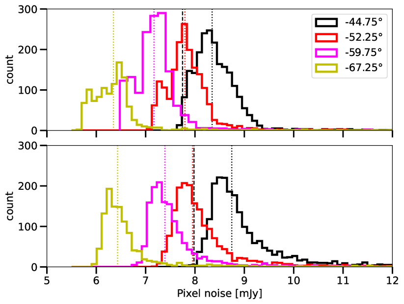
Figure 1: Histograms of noise values for every observation processed in the archival transient pipeline, grouped by subfield. Histograms are colored by subfield and referred to by the center declination of that subfield. The noise value for each observation is the median pixel noise across all the pixels in the corresponding skymap. The top and bottom panes show the noise values for the 95 GHz and 150 GHz maps, respectively. Dotted colored lines mark the median noise across all observations within a given subfield, while the dashed black line shows the overall median across all observations.

2.2 Transient Finding

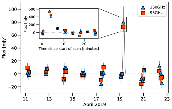
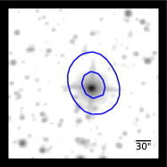
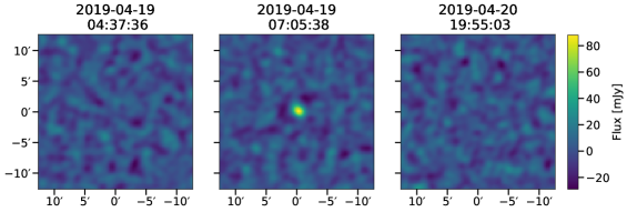
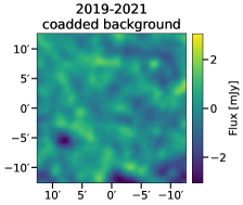
Figure 2: Example lightcurves and thumbnails for the SPT event on MJD 58592.3. Top left: Lightcurves for the highest TS pixel on the triggered event. The main plot shows the peak single-observation flux while the inset shows the single-scan flux within the peak single-observation. Top right: unWISE 3.4 $\mu$m W1 grayscale image (Lang, 2014) with blue SPT $150\text{\,}\mathrm{GHz}$ flux density contours in 5$\sigma$ steps from the peak signal. Bottom: $150\text{\,}\mathrm{GHz}$ thumbnails for the single-observation data points (immediately before, during, and immediately after the triggered event), and the three-year average map that has been subtracted to create these thumbnails. These thumbnails show that this flaring star is undetectable in single SPT-3G observations at its quiescent level.

The transient finding method is described in detail in Guns et al. (2021) and we provide a brief overview here as well as noting any pertinent changes. For each unmasked location on the pixelated sky, we construct a series of two-band lightcurves spanning consecutive 12-day intervals and using only $95\text{\,}\mathrm{GHz}$ and $150\text{\,}\mathrm{GHz}$ data. The 12-day interval covers short-duration signals of interest – millimeter stellar flares from previous and ongoing analyses (i.e. Guns et al., 2021) as well as predicted short duration extragalactic millimeter transients (Eftekhari et al., 2022). We apply a preliminary cut on the data, selecting all lightcurves which show a $>$3$\sigma$ excursion in both bands at the same point in time. To each remaining lightcurve we fit a four-parameter Gaussian flare model with two independent flux parameters $S_{95}$ and $S_{150}$ at 95 and $150\text{\,}\mathrm{GHz}$, a peak time $t_{0}$, and an event full width at half maximum (FWHM) $w$. The Test Statistic (TS) is constructed by maximizing the likelihood ratio of the best-fit flare model to the null model (zero amplitude in both bands), with an additional logarithmic penalty term. This penalty term corrects for a likelihood bias towards short flare widths: since there are many more uncorrelated starting times for short flare widths than for long ones, the effective volume of searchable parameter space grows as the flare width decreases. The logarithmic penalty term effectively imposes a flat prior on the flare duration in order to correct for this effect (Braun et al., 2010).

The TS is thus defined as:

$$\mathrm{TS}=2\,\mathrm{ln}\mathcal{L}\left(\hat{S}_{95},\hat{S}_{150},\hat{t}_{0},\hat{w}\right)-2\,\mathrm{ln}\mathcal{L}(0)+2\,\mathrm{ln}\left(\frac{\hat{w}}{12\ \text{days}}\right),$$ (1)

where hatted quantities denote best-fit parameters as found by a non-linear optimizer using the Nelder-Mead simplex method, as implemented in the GNU Scientific Library (Galassi et al., 2009).

Focusing our search on short-duration events, we impose a significance cut of TS $>45$ and a best-fit FWHM duration $<10$ days. The TS cut is set by demanding a negligible background of false detections from background noise ($\ll 1$ events over four years [S. Guns et al, in preparation]). In the short duration regime, the main systematic background for SPT transients are weather balloons that are launched daily by the South Pole Meteorological Office (Met). Through a data sharing agreement established in 2022, SPT now receives Met GPS data soon after each balloon launch and cuts any telescope scans that intersect with a weather balloon trajectory, vastly reducing the number of detected balloons in the SPT-3G transient detection pipeline at the cost of a negligible reduction in data volume. The balloon avoidance system is not infallible however, and fails when the tracking data arrives too late to be integrated into the SPT-3G data processing pipeline, or when the balloon ruptures at high altitude and debris that is not tracked by the balloon’s GPS module enters the SPT-3G field of view. Remaining balloon detections number approximately one per month and are identified by their observational signature: due to their fast movement they are detected with a short duration in single telescope scans (lasting 2 or fewer seconds), high brightness ($>1$ Jy), thermal or steeper-than-thermal spectra, and within 2 hours of a logged balloon launch.

After removing events with best-fit durations $>10$ days and TS $<45$ we are left with a dataset of candidate events which we inspect by eye. We manually analyze the lightcurves and thumbnails to reject duplicate observations of the same event, filtering artifacts from bright nearby transients, untracked balloons, and detector glitches (large map streaks in the scan direction). Events with any ambiguity are excluded from further analysis. After these cuts, we keep 111 short duration ($<10$ day) events with robust morphologies that we use to cross-match to the Gaia Data Release 3 (DR3) catalog (van Leeuwen et al., 2022).

Figure 2 shows an example event detected by the transient pipeline. The main lightcurve plot shows the data that is input into the lightcurve fitter and the resulting Gaussian fit, with a TS of 194.8. Each data point represents the average flux over a 2-hour SPT subfield observation, in which any given point on the sky is observed for about 8 consecutive left/right scans (16 scans total) over the course of 20 minutes. We construct post-detection lightcurves of the single-scan fluxes (each scan representing one pass of the focal plane, or roughly 2 seconds of integrated data) that make up the peak observation of the flare, shown as an inset to the main lightcurve. Figure 3 shows thumbnails of the single-scans for this event. Thumbnails of scans 1, 2, 19, and 20 are discarded because the sky location of interest is not observed by the focal plane. Scans at the beginning and end (such as scans 3 and 4) are noisier due to only part of the focal plane seeing the sky location of interest.

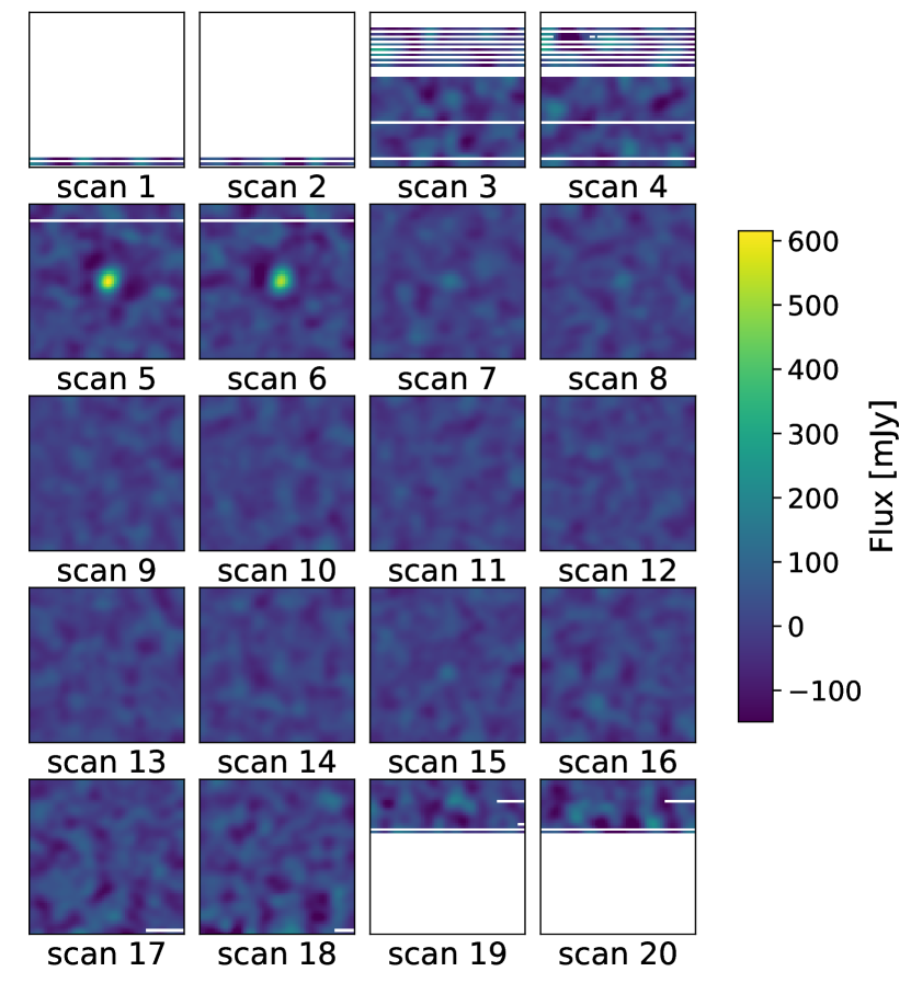
Figure 3: $15\text{\,}\arcsec$x$15\text{\,}\arcsec$ single-scan $150\text{\,}\mathrm{GHz}$ thumbnails centered on the highest TS pixel from the event in Figure 2. The source is only clearly visible in scans 5 and 6, and has returned to near noise flux values in scans 7 and 8.

In order to localize events at finer scales than the $15\text{\,}\arcsec$ pixel grid, we determine an event centroid location from the TS map associated with each flare. The TS map is constructed by fitting the lightcurve model to each pixel in a 5x5 pixel ($1.25\text{\,}\mathrm{\SIUnitSymbolArcminute}$x$1.25\text{\,}\mathrm{\SIUnitSymbolArcminute}$) box centered on the event. The TS map combines all the available information from every time point and both frequency bands (under the assumption of a Gaussian flare model). For each event, we fit a cubic spline to to the TS map and choose the spline maximum as the event location.

The uncertainties in the SPT R.A. and decl., $\sigma_{\text{RA}}$ and $\sigma_{\text{Dec}}$, come from a combination of systematic pointing uncertainty and statistical uncertainty in localizing a source given the SPT beam and noise:

$$\sigma_{RA}^{2}=$3.73\text{\,}\arcsec$^{2}+\left(\frac{$50\text{\,}\arcsec$}{\sqrt{TS}}\right)^{2},$$ (2)

$$\sigma_{Dec}^{2}=$4.35\text{\,}\arcsec$^{2}+\left(\frac{$49\text{\,}\arcsec$}{\sqrt{TS}}\right)^{2}.$$ (3)

The first term is the systematic contribution to the error budget and comes from uncertainties in the pointing of the physical instrument, whereas the second term is the statistical contribution, and is sourced by the noise in the observations. We estimate the first term by measuring the positions of one year of daily observations of bright point sources and comparing to a reference catalog. The second term is calculated from injecting N=10,000 simulated sources of various amplitudes at known locations in the SPT field and recovering the measured position. In a small fraction ($<$1%) of cases, heavy winds and other inclement weather leads to systematic pointing errors that are much larger than the mean estimate in Equations 2 and 3. In those cases, we estimate the systematic pointing error from the bright point source positions as measured in that observation only.

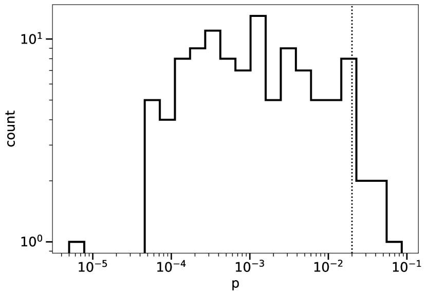
Figure 4: The distribution of p-values from matching SPT flaring events to stars in the Gaia DR3 catalog. The 5 events at p$>$0.02 have been investigated and are discussed in Section 3.8.3.

3 Results

Column	Label	Units	Description
1	spt_id		IAU-approved SPT source name, corresponding to the SPT detected location.
2	mjd	[days]	The approximate time in MJD corresponding to the beginning of the observation the detection took place in.
3	ts		The test statistic of the event, used to flag a possible flaring event occurring during that observation. Minimum values are 45, with a higher value having a more significant detection.
4,5	ra	[deg]	The R.A. and Declination (J2000) of the SPT event.
	dec
6-11	95_flux	[mJy]	Flux values and their errors for the three SPT bands.
	95_flux_err
	150_flux
	150_flux_err
	220_flux
	220_flux_err
12-15	spectral_index_95_150		2-band spectral index values and their errors for the 95/150
	spectral_index_95_150_err		and 150/220 SPT bands.
	spectral_index_150_220
	spectral_index_150_220_err
16	dr3_source_id		Gaia DR3 unique source identifier.
17	p		The probability of a random event cross-matching to this source.
18,19	source_ra	[deg]	The R.A. and Declination (J2000) of the Gaia DR3 source.
	source_dec
20-22	phot_g_mean_mag		Magnitudes of the three Gaia passbands.
	phot_bp_mean_mag
	phot_rp_mean_mag
23,24	parallax	[mas]	Parallax and error of the Gaia source.
	parallax_err
25	binary		Boolean flag for binary candidacy.
26	2rxs_id		2RXS identifier.
27	2rxs_ref		Flag for source association: “Freund” for an established association, or “DR3/2RXS Proximity” for nearby sources.
28	2rxs_flux	[mW m-2]	2RXS flux.

Table 1: Columns and descriptions for the SPT-3G flare star catalog.

3.1 Stellar Association

3.1.1 Candidate Sources

To find candidate stars for our events we only consider Gaia sources within our observing field that have a maximum G magnitude of 20 and exclude sources that are found in the qso_candidates or galaxy_candidates tables in Gaia DR3 to eliminate known extragalactic sources. This leaves about 7.3 million stars as possible matches for SPT-3G transients. X-ray associations with sources from the second ROSAT all-sky survey (2RXS) are provided by the main table of the ROSAT stellar content catalog (Freund et al., 2022), matching only on Gaia DR3 source ID. For Gaia stars without a match in the stellar content catalog, we check the full 2RXS point source catalog (Boller et al., 2016) for any sources within $1\text{\,}\mathrm{\SIUnitSymbolArcminute}$ and have separately distinguished them.

3.1.2 Cross-Matching Algorithm

To associate flaring events with sources, the cross-matching algorithm we use compares the likelihood of an event originating from a candidate source to the likelihood of a random event having a chance association, using a $1\text{\,}\mathrm{\SIUnitSymbolDegree}$ radius centered on each candidate to determine a local source density in the Gaia catalog. This results in the figure of merit in association $\Lambda$:

$$\Lambda=\ln\left(\mathcal{B}\frac{N_{\text{total}}}{N(>\text{S})}\right),$$ (4)

where $N_{\text{total}}$ is the number of sources within the local area, and N($>$S) is the number of sources within the local area that are brighter in Gaia magnitude than the candidate source. $\mathcal{B}$ considers the uncertainties of the SPT beam and the angular separation:

$$\mathcal{B}=\exp{\left[-\frac{1}{2}\left((\frac{\Delta_{\text{RA}}}{\sigma_{\text{RA}}})^{2}+(\frac{\Delta_{\text{Dec}}}{\sigma_{\text{Dec}}})^{2}\right)\right]}.$$ (5)

$\Delta_{\text{RA}}$ and $\Delta_{\text{Dec}}$ are the angular separations in R.A. and decl. between the transient centroid location and candidate source in the Gaia catalog while $\sigma_{\text{RA}}$ and $\sigma_{\text{Dec}}$ are defined in Equations 2 and 3.

We create a probability distribution function for random matches by sampling 400,000 random points in the SPT-3G field and matching them to Gaia using this algorithm. We then construct a cumulative distribution function (CDF) based on the distribution of $\Lambda$ values for this random sample, and then create a one-to-one mapping of $\Lambda$ to p-values in the form of $p(\Lambda)=1-\text{CDF}(\Lambda)$. We interpolate this mapping to find the p-value corresponding to the observed $\Lambda$ for each event, telling us the chance of a random event having that same association value or higher. The distribution of p-values for our events is shown in Figure 4.

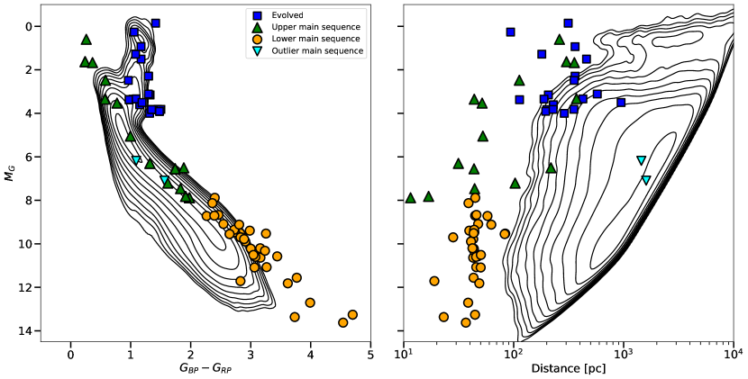
Figure 5: Left: CMD of SPT flaring stars, with contours showing density of Gaia stars in the SPT-3G winter field. Right: Magnitude vs distance of the same populations. The two inverted triangles are outlier main sequence stars and considered to be incorrect matches, which are discussed in Section 3.8.3.

3.2 SPT-3G Flare Star Catalog

As described in Section 2.2, this flare star catalog is a result of searching only for short-duration transient events in SPT-3G archival data, using a cutoff of 10 days on the best-fit FWHM duration. With our current analysis we have recovered 12 of the 13 stellar flaring events in Guns et al. (2021), and include them in the flare star catalog. The missing flaring event, previously referred to as event 6(a) by the star CC Eri, was a weak flare detected at 29/21 mJy in the 95/$150\text{\,}\mathrm{GHz}$ bands with respective luminosities of 4.4$\times$10²⁶/5.0$\times$10²⁶ erg s^-1 and a TS of 29.5, below the current detected threshold of 45. The other flares from CC Eri were successfully recovered. The previous analysis in Guns et al. (2021) had a detection threshold of TS $=100$. Any location in the sky exhibiting a flare with a TS $\geq 100$ was then manually scrutinized over the entire observing season to see if there were smaller flares below the threshold that were not detected. This method was how event 6(a), at TS $=29.5$, was found originally. We do not search for below-treshold flares in the current analysis and only show events above the new TS $=45$ threshold. The two long duration events from Guns et al. (2021) are longer than the 10 day best-fit FWHM cut and thus were not recovered.

Table 1 shows the full column names and descriptions for the flare star catalog. A full machine readable table can be found at https://pole.uchicago.edu/public/data/tandoi24/.

After matching with the external catalogs described in Section 3.1.1, the full 4 year SPT flare star catalog has associated all 111 flaring events with 66 unique stars. We find that 17 stars have flared multiple times and are responsible for 62 events, leaving 49 stars with single events associated with them. Distances for stars are derived from Gaia DR3 parallax when available. 5 stars, associated with 6 events, have no reported parallax from Gaia. Table 2 shows alternate sources of parallax, or distance if parallax is not available.

Gaia DR3 ID	Parallax [mas]	Distance [pc]	Source
4914632365579875200	21
4726387007013852672	59 $\pm$ 1
6580179279486143744		44 $\pm$ 2
4850405974392619648		44 $\pm$ 1
4942856382389905408		19 $\pm$ 4

Table 2: Alternate sources for parallax or distance for stars that have missing parallax in Gaia, with rounded values.

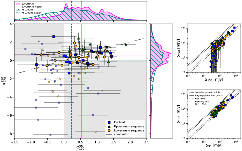
Figure 6: Left: Spectral indices for all stellar flare events, with KDEs of the probability densities along the insets. Shaded regions mark separate quadrants of positive and negative values of alpha, while the dotted line indicates a spectral index that is constant in frequency. Events with 220 GHz SNR $<3\sigma$ have their $y$-error bars omitted and marker sizes reduced for visual clarity. These spectral indices are within the typical values for synchrotron radiation more commonly seen at radio wavelengths. Right: Comparisons of flux densities for all stellar flare events, across the three SPT bands. Typical spectral indices of relevant phenomena are shown as lines.

Figure 5 shows the population of SPT detected flare stars with Gaia parallax in a color-magnitude diagram (CMD), and a magnitude vs distance plot. Different marker shapes denote our classifications of spectral types with “Evolved” containing giants and subgiants, “Upper main sequence” containing early-type and sun-like stars, and “Lower main sequence” mainly composed of M dwarfs. These classifications are based purely on position in the CMD. We note that these classifications may be inaccurate due to the possibility of misrepresenting a binary system which we discuss in Section 3.8. In addition, the two main sequence outlier stars which we show in Section 3.8.3 are likely misidentifications and are not used in analysis.

M dwarf stars, having a Gaia $G_{BP}-G_{RP}$ color of $>\sim$2.1 are interesting due to both their tendency for large and frequent flares (France et al., 2016) and abundance — accounting for $\sim 75\%$ of stars in our local neighborhood (Bochanski et al., 2010). The M dwarf population that the SPT has seen flare is largely above the main sequence, indicating these could be young stars that have not yet settled onto the main sequence.

Early type stars (spectral types B5-F5 with a Gaia $G_{BP}-G_{RP}$ color of $<\sim$0.5) are also represented in the SPT flaring population. While initially believed to not exhibit flares, there has been recent evidence of flaring activity in early type stars at other wavelengths (Balona, 2012; Van Doorsselaere et al., 2017). The upper main sequence stars that have been detected flaring by SPT are generally closer in distance than typical main sequence stars. This could indicate that flaring in these types of star could be very common, and SPT is preferentially detecting the sample that happens to be nearby.

3.3 Spectral Index

Spectral indices for the events are shown in the main plot in Figure 6. Events are separated by their $220\text{\,}\mathrm{GHz}$ SNR, with a focus on events with strong ($>3\sigma$) detections. Events with weak $220\text{\,}\mathrm{GHz}$ SNR have their $y$-error bars omitted and marker sizes reduced for visual clarity.

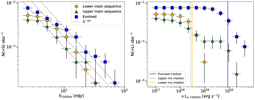
Figure 7: Cumulative number counts per SPT observation for flaring events at $150\text{\,}\mathrm{GHz}$. Left: Number counts as a function of source flux densities. Dashed lines are examples of the Euclidean source count expected power law of $S^{-3/2}$. Right: Number counts as a function of peak flare luminosities. Vertical lines show the median luminosity value for each population of stars.

The spectral indices are defined through the relation:

$$S_{\nu}\propto\nu^{\alpha},$$ (6)

such that

$$\alpha^{\nu_{1}}_{\nu_{2}}=\frac{\log(S_{1}/S_{2})}{\log(\nu_{1}/\nu_{2})}.$$ (7)

To represent probability densities of the observed spectral indices, we have calculated kernel density estimations (KDEs) for two populations: a KDE for the subset of events with strong $220\text{\,}\mathrm{GHz}$ detections as well as a KDE for the entire population of flaring events regardless of $220\text{\,}\mathrm{GHz}$ SNR, in both $\alpha^{95}_{150}$ and $\alpha^{150}_{220}$. Gaussian kernels are used with the width set by the uncertainty on the spectral index measurement. We show these KDEs along the x- and y-insets, as well as median spectral index values for the two populations.

Most of the events detected by SPT cluster around the constant spectral index line, with median spectral indices of $\alpha\approx$ 0 to 0.5. Measurements of $\alpha$ generally do not exceed 5/2 which is the spectral index for optically thick synchrotron radiation (Pacholczyk, 1970), but most do not seem consistent with a falling spectrum expected for the optically thin side of synchrotron radiation that peaked at radio wavelengths around $\sim$5 GHz.

In the flux subplots, spectral indices with typical values in the radio regime are marked with black lines. $\alpha=-0.75$ represents an optically thin synchrotron source, $\alpha=0$ represents a flat spectral index, $\alpha=2$ represents the Rayleigh-Jeans tail of thermal emission, and $\alpha=5/2$ represents an optically thick synchrotron source due to self-absorption. The SPT detected events fall within the bounds of typical synchrotron spectra for $\alpha^{95}_{150}$ as well as $\alpha^{150}_{220}$, suggesting this as a plausible emission mechanism.

3.4 Number Counts

Figure 7 shows cumulative number counts of both flux density and $150\text{\,}\mathrm{GHz}$ peak flare luminosity, split for the three populations of stars we have established.

The flux density number count can be approximated as a power law of $N\left(>S\right)$ $\approx$ $S^{-3/2}$ where the index comes from assuming a uniform density of objects within a sphere: $N\propto r^{3}$ and $S\propto r^{-2}$. This approximation is shown as a series of dashed lines in the flux density number count plot. At distances that exceed the thickness of the galactic disk the power law approximation will break down. The lower main sequence stars are $<100$ pc in distance and are not detected outside of the disk. However, the evolved stars are seen at distances up to 1 kpc and may be detected at distances where a drop in density is expected.

The luminosity number count shows that the main sequence stars have similar luminosity distributions, while the evolved stars have much brighter flares as well as higher flaring rates in comparison. Incorporating the transient detection efficiency results of flares lasting 30 minutes or less as discussed in Section 2.1, we find an expected flaring rate N$\left(>\text{L}\right)$ deg^-2 yr^-1 of 0.2/0.3/0.4 for the upper main sequence/lower main sequence/evolved populations of stars at a $\nu L_{\nu}$ $150\text{\,}\mathrm{GHz}$ luminosity of $10^{27}$ erg s^-1.

3.5 X-ray

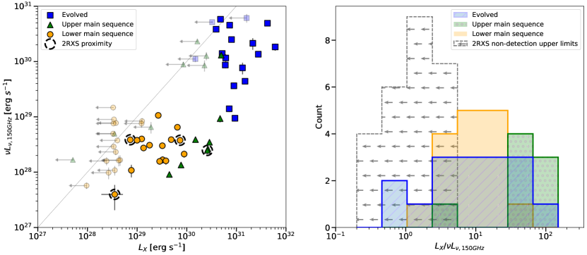
Figure 8: Left: Comparison of mm flaring and X-ray quiescent luminosities. A dotted line shows equal luminosities, and SPT-detected flare stars without a 2RXS association are shown as transparent markers at the luminosity corresponding to the mean X-ray flux upper limit of $1.5\times 10^{-13}$ erg s^-1 cm^-2 calculated in Freund et al. (2022). Right: A histogram of luminosity ratios for the three populations of stars that have 2RXS associations through Freund et al. (2022) and proximity to objects in Boller et al. (2016). Stars without an X-ray association are binned by their upper limits and are marked with arrows pointing left. These plots show a wide spread in the ratio of quiescent SXR to flaring mm-wave luminosities.

Studies of the Sun and other active main sequence stars have shown that a linear relationship exists between soft X-ray (SXR) emission and magnetic flux (Pevtsov et al., 2003), linking thermal coronal emission to magnetic fields. Flaring rates and luminosity have been linked to quiescent SXR emission (Audard et al., 2000) as well as other proxies for stellar magnetic activity such as H$\alpha$ emission and rotation period (Davenport, 2016; Yang et al., 2017).

Figure 8 shows the SPT flaring stars at $150\text{\,}\mathrm{GHz}$ along with quiescent SXR (0.1-2.4 keV) from 2RXS in luminosity, as well as a histogram of the ratios of luminosity. Stars that are not associated with any 2RXS sources are shown as faint markers at an approximate upper limit of $1.5\times 10^{-13}$ erg s^-1. The upper limit is only a rough estimate: the exposure time strongly varies and thus no uniform detection limit exists (Freund et al., 2022). Additionally, four sources not matched in Freund et al. (2022) but within $1\text{\,}\mathrm{\SIUnitSymbolArcminute}$ of sources included in Boller et al. (2016) are shown with a dashed circle around the marker. Their flux ($F_{X}$) is calculated following Schmitt et al. (1995) using the hardness ratio (HR) and photon count rate (ctr):

$$F_{X}=(5.30\text{HR}+8.31)\text{ctr}\times 10^{-12}\text{ergs cm}^{-2}\text{s}^{-1}.$$ (8)

We have used this equation to recover the same flux values for sources given in Freund et al. (2022), using the hardness ratios and photon count rates supplied within.

Considering only the SPT-detected flare stars with an association in 2RXS (i.e., excluding the matches within $1\text{\,}\mathrm{a}\mathrm{r}\mathrm{c}\mathrm{m}\mathrm{i}\mathrm{n}$ proximity), the percentage of stars that are X-ray bright is 54.5%. For comparison, we select a population of 330 stars that are representative of the SPT flaring star population. Using the parameters of magnitude and distance (see the right plot in Figure 5), we selected 5 nearest neighbors for each SPT flare star. The nearest neighbor stars have a percentage of X-ray bright stars of 4.8%. These rates provide evidence that stars observed to flare at mm wavelengths are much more likely to be X-ray bright than non-flaring stars.

The histograms in Figure 8 show a large scatter in the ratio of quiescent SXR luminosity to mm-wave flaring luminosity for the population of stars with 2RXS associations. Simultaneous observations of SXR and mm-wave emission during flaring states may reveal a tighter correlation between these luminosities.

3.6 Single-Scan lightcurves

Flare morphologies on short timescales can tell us about the physics of the flare. However, binning or gaps in data can obscure important features of these flares. At optical wavelengths, higher cadence observations from TESS have shown a degeneracy in data even at the 2 minute scale with subsequent pulsations after the peak and during the decay phase possible in a larger portion of the population (Howard & MacGregor, 2022).

Lightcurves at radio wavelengths typically describe the impulsive phase of the flare, but a phase of gradual change at these wavelengths has also been detected (Zhang et al., 2018). The impulsive stellar flare lightcurve seen in radio, optical, and HXR wavelengths is characterized by a sharp rise followed by an exponential decay with some small complexities occurring during both phases (Davenport et al., 2014; Kowalski et al., 2019). Different types of stars can also exhibit unusual flare morphologies: flares from RS CVn binary systems have longer rise times and sustained peak emission that plateaus before decaying (Osten & Brown, 1999).

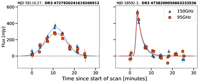
Figure 9: Possible stellar flare models on well-constrained single-scan lightcurves. As shown in the appendix, most flares detected by SPT are not as clear in their structure. Both of these lightcurves are of flares from lower main sequence stars. Left: A simple Gaussian model showing a gradual rise in flux that is comparable to the decay period. Right: A sharp Gaussian rise with a longer exponential decay.

Flaring activity can also trigger additional flares in neighboring active regions of the star in a process known as sympathetic flaring. Sympathetic flaring has been observed on the Sun (Pearce & Harrison, 1990), with evidence of this phenomena happening in other stars (Anfinogentov et al., 2013). This could explain the appearance of a complex flare as the superposition of separate flares on the surface of the star.

Most descriptions of the duration of stellar flares at shorter wavelengths benefit from higher cadence observations, longer times spent viewing the star, or some combination of both. Due to the SPT scanning strategy, we are limited to the binned single-scan data points roughly 100 seconds apart on average with the actual time spent on a given sky location depending on where that location falls in the focal plane’s approximately oval shape. As these are not targeted observations, we rarely observe the duration of a flare in its entirety. Such observations can only give us a lower limit on the duration of these events.

Figure 9 shows lightcurves of 2 events with clear morphologies, including including a long Gaussian rise time and an exponential decay. Visual inspection resulted in around 15 detected flares being considered to have clear structure, while most flares did not have a well defined evolution of the lightcurve during the time observed. Additional single-scan lightcurves for all SPT stars are included in the appendix; these lightcurves also contain $220\text{\,}\mathrm{GHz}$ data which has approximately 5$\times$ higher noise than the 95 and $150\text{\,}\mathrm{GHz}$ bands.

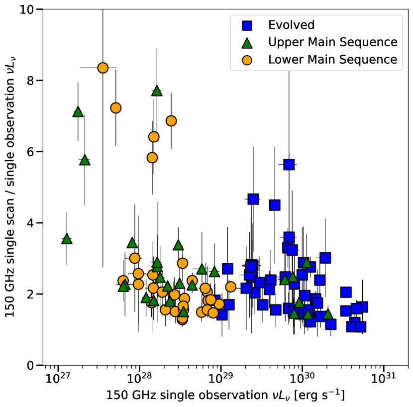
Figure 10: Comparison of single-scan and single-observation peak $150\text{\,}\mathrm{GHz}$ luminosities for each event. The flux values from observations are a factor of  2 lower than the peak from single-scans for the majority of flares.

The peak flux values of flares reported in the catalog are averaged over full observations and thus have a lower peak flux value than the corresponding single-scan lightcurve. Shorter duration events have larger biases since typical observations contain 16 single-scan data points. An event that is shorter than 100 seconds in duration may only be caught in one single-scan and will be reduced by a factor of 16 when using the single-observation flux instead. We choose to represent the stellar flares with single-observation flux values due to our transient detection pipeline running on single-observation lightcurves as well as the increased noise values inherent to the single-scan data. Figure 10 shows the difference in $150\text{\,}\mathrm{GHz}$ luminosities for flares using peak single-observation and peak single-scan fluxes, showing that the average difference in recovered luminosity is roughly a factor of 2.

Our single-scan lightcurves occasionally have additional peaks in them. When considering the typical duration for the impulsive phase of a stellar flare on the order of seconds, we can not confidently classify these peaks as a separate event occurring nearby temporally, or a pre/post flare pulsation as described in Howard & MacGregor (2022) where similarly binned TESS data at 120 second cadence is sufficient enough time to hide structure of the flare morphology.

3.7 Flaring Activity Durations

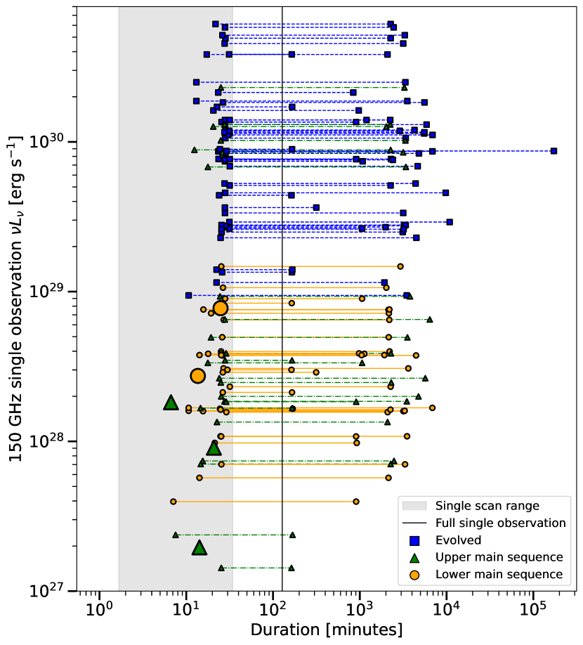
Figure 11: Constraints on durations for stellar flares, using single-scan lightcurves to determine lower limits and single-observation lightcurves to determine upper limits. 5 events are found to be fully contained within the single-scan lightcurve and have single markers at a larger size.

We constrain the duration of flaring activity by using the single-scan and single-observation lightcurves for each event. Lower limits on duration are set by the single-scan lightcurve, with a flare considered to be at quiescence (either before or after the peak) by having a single-scan SNR below 4$\sigma$ simultaneously in both bands. For a flare to be considered fully contained within a single-scan lightcurve, quiescent points need to exist on either side of the flare. For flares with only one quiescent point in their single-scan lightcurve, the minimum duration is considered to be from this quiescent point to either the beginning or end of the lightcurve depending on where it is in relation to the peak. Flares with no quiescent points in their single-scan lightcurve use the full time between the first and last scan as a minimum duration. Upper limits on duration are constrained in a similar way: quiescence is considered to be when the closest single-observation returns to 1$\sigma$ before and after the peak.

Figure 11 shows the constraints on duration for all flaring events. We find 5 flares to be fully constrained within the single-scan lightcurve and have measured their durations: these are plotted as larger marker sizes with an uncertainty of one full single-scan (100 s). The shaded area denotes the range in possible times that a location will be observed by the SPT, from one scan (100 s) to 20 scans including the time for the SPT to accelerate and change elevation while it is not collecting data (2060 s). The vertical line shows the typical duration of a full single-observation (7668 s).

Going from single-observation to single-scan lightcurves increases our time resolution, but still suffers a low cadence, as there are 100 seconds on average between data points. Depending on where in the subfield the flaring event occurs, subsequent single-scan data points may represent just a few seconds of the focal plane passing over that part of the sky (see Figure 3), with large gaps in time possible as it takes the telescope 100 seconds to complete a scan in one direction. This cadence is more than sufficient to hide features in a flare.

Similarly, large gaps between single-observation data points can span anywhere from 2 to 24+ hours depending on the subfield observation schedule. For most flares, these temporal gaps in SPT data are large enough that it is likely that the true duration of the flare is much closer to the lower limit. Some flares exhibit multiple single-observation data points that are likely part of the same long duration flare, but could also possibly be separate back-to-back flares. The transient detection pipeline only fits for a single flare in each 12-day lightcurve, so additional flares in the same lightcurve will go unreported. Lightcurves for all events have been manually analyzed for obvious secondary flares and none have been found. This fitting method will be improved on in the future to allow for finding multiple flares within the same lightcurve.

3.8 Additional Classifications

3.8.1 Binary Systems

We have checked for binarity in the sample of SPT-detected flare stars. Binary systems can lead to confusion in determining the correct source — there is a possibility of matching to the wrong star due to undetected secondaries or preferentially selecting the brightest star in Gaia. Stars in binary systems can also exhibit flares due to interactions between the stars, such as RS CVn systems which have been detected at millimeter wavelengths (Brown & Brown, 2006) and are known to flare frequently (Osten & Brown, 1999).

Using Vizier (Ochsenbein et al., 2000), we have searched all flaring stars for inclusion in catalogs of binary stars as well as classification by Gaia (Rimoldini et al., 2023). We use the same process described in Section 3.5 to compare SPT-detected stars to a similar representative population in Gaia.

We find that the SPT population of stars is over-represented in RS CVn classification by Gaia (10.6% compared to 0.6% for the nearest-neighbor population) as well as probable binary candidates (51.5% compared to 22.7%). While many of these classifications require more definitive proof such as spectroscopic observations, this propensity for binarity could be important to the underlying mechanisms found in millimeter flares.

3.8.2 Multiple Flares

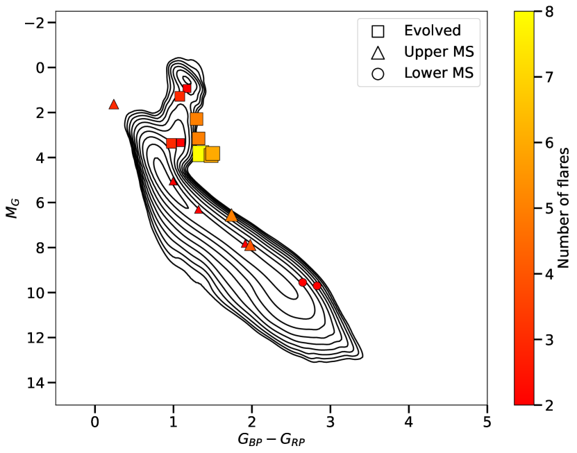
Figure 12: Gaia CMD showing stars that have multiple flares detected by the SPT. Colored and marker size scaled by number of flares. Most of the multiple flares detected originate from evolved stars.

Figure 12 shows a CMD of the stars we have detected flaring multiple times. While these stars sample the entirety of our population, we find that our detections of multiple flares are dominated by evolved stars with 30 of the 62 events coming from just 5 stars. From preliminary simulations of injected flare efficiency (Section 2.1), it is likely the true rate of above-threshold flares from these stars ranges from 2$\times$ to 20$\times$ higher than observed. Figure 11 shows only 5 flares — from upper and lower main sequence stars — to be fully constrained and to have durations on the scale of 30 minutes or less, suggesting the main sequence stars in Figure 12 have a true flaring rate closer to 20$\times$ higher. Table A1 shows a full listing of these stars and all of their associated events.

3.8.3 Outlier Events

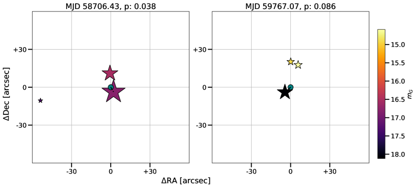
Figure 13: Two events with outlier distances and their potential Gaia matches shown at their angular separation. Stars represent candidate sources, and are colored by brightness and sized scaling inversely with p-value.

Flaring events in Figure 4 having p-values greater than 0.02 have been individually investigated. In most cases the higher than typical p-value is due to the associated star being in a high local density region and having multiple nearby candidate stars, and we believe these matches to be correct.

Figure 13 shows the local Gaia density for the two events on MJD 58706.43 (p: 0.038) and MJD 59767.07 (p: 0.086). For both of these events, our cross-matching algorithm picked a dimmer star closer in angular separation rather than brighter stars at slightly larger separation. In addition, both events are matched to extreme outliers: they are main sequence stars at distances over 1kpc, significantly further away than other stars we match to. Figure 5 shows these two anomalous stars in the middle of the main sequence as having much further distances than similar main sequence stars the SPT has detected, resulting in extremely high flaring luminosities. For both of these events, the other potential candidates are nearby M Dwarfs: the candidate for MJD 58706.43 is a potential binary system (Reiners et al., 2010), and the two candidates for MJD 59767.07 have an angular separation of $6.2\text{\,}\arcsec$ and distances of 51.13 and 51.17 pc giving a distance from each other of $\sim$0.04 pc. We believe that the M Dwarfs are a more likely match for both events, and have changed the associated sources.

These cases suggest some improvements in our cross-matching algorithm can be made. The events were preferentially matched to a distant main sequence star — rather than a brighter M Dwarf at slightly higher angular separation — it is possible that including a prior on parallax based on our confirmed distributions in the CMD can steer the event to a more plausible match. Likewise, incorporating a prior that favors stars that have been observed flaring previously might be considered. Further optimization of this algorithm will be necessary to inform future analysis of surveys such as CMB-S4 and SO, and especially for surveys that include the galactic plane.

4 Conclusion

We have presented a new catalog of short duration ($<$10 days) transient events found in a non-targeted SPT-3G survey using an updated transient detection and matching method. This catalog is produced from analyzing 4 years of daily observations of a 1500 square degree field at 95 and $150\text{\,}\mathrm{GHz}$ by the SPT-3G survey, with the inclusion of $220\text{\,}\mathrm{GHz}$ data coming after events have been detected. The catalog is are provided in machine readable format at https://pole.uchicago.edu/public/data/tandoi24/, along with 4-year single-observation lightcurves at 95 and $150\text{\,}\mathrm{GHz}$ of each unique star, and single-scan lightcurves at 95, 150, and $220\text{\,}\mathrm{GHz}$ of each flaring event.

We have found that two-band spectral index comparisons for 95/150 and 150/$220\text{\,}\mathrm{GHz}$ generally fall between an optically thick synchrotron spectrum ($\alpha$=5/2) and a typical value of the optically thin tail of synchrotron ($\alpha$=-0.75). While optically thick synchrotron radiation typically peaks at radio frequencies ($\sim$5 GHz), evidence of rising spectra at sub-mm frequencies have been observed in solar flares.

We have found these flaring events to be nearby stars that we have matched to Gaia Data Release 3. Many of these stars have counterparts in the 2RXS stellar content catalog. A CMD shows our population of matched stars, indicating that we are seeing flaring events from stars spanning a wide range of spectral types with most of these flares occurring in M Dwarfs and along the Giant branch.

Quiescent SXR emission has been shown to have a linear relationship with magnetic flux in main sequence stars, assumed to be the cause for the flaring activity we have observed, along with measures of direct flaring activity. We have shown quiescent SXR emission along with peak flare $150\text{\,}\mathrm{GHz}$ luminosity, and a comparison of this ratio, and found strong evidence that mm-wave flaring stars tend to be quiescently bright in SXR. A wide spread in this ratio exists that may be tightened up with simultaneous SXR and mm emissions during a flare.

We have shown cumulative number counts of the flaring stars in flux densities and peak flare luminosities. The flux density number count has a slope consistent with observing sources in a uniform density, i.e. the Milky Way disk, at higher flux values, with this assumed power law of $N\left(>S\right)$ $\approx$ $S^{-3/2}$ breaking as flux density approaches the SPT transient detection threshold. The number count as a function of luminosity shows lower and upper main sequence stars having similar median luminosities. Evolved stars have a median peak flare luminosity over one magnitude brighter than the SPT-detected main sequence stars.

We have flagged all probable binary system candidates, known through Gaia variability tables and a literature search in Vizier. It is not clear if these flares originate from the associated star, a companion, or an interaction between the stars in the system.

We have observed 17 out of 66 stars flare multiple times, comprising over half of our events and a wide range of spectral types, with most of these multi-flare events originating from just a few evolved stars.

We believe that our cross-matching algorithm has erroneously matched two events with distant stars resulting in anomalously high luminosities. Both matches are to main sequence stars at distances of $>$1 kpc (greater than any other Gaia star that SPT has observed flaring) and are closer in angular separation to the SPT event compared to nearby M Dwarfs at $\approx$ 50 pc which are brighter in apparent magnitude. We believe that the M Dwarfs are the source of the flaring activity for both of these events. In the future, we are considering adding a prior based on location in the Gaia CMD to our cross-matching algorithm.

We have shown finer time resolution single-scan lightcurves of events, using these as a lower limit constraint on durations. Upper limits on the duration are found using single-observation lightcurves and we have found typical constraints on duration range from $\sim 10^{1}$ to $\sim 10^{4}$ minutes. These constraints are weak, and are generally dominated by the SPT observation cadence. Two potential models are shown to fit to some of the shorter duration single-scan lightcurves: a sharp rise with exponential decay, and a Gaussian fit with a rise time comparable to the decay time.

Simultaneous observations will be possible for future SPT observing seasons with TESS having revisited the SPT-3G field in July 2023, and the ASKAP Variables and Slow Transients (VAST) survey covering the same area of the sky over parts of the next few years. With additional wavelengths, and polarization in the case of VAST, these surveys will deliver important information as to the nature of these flaring events. Targeted observations of known multi-flaring SPT stars from radio instruments such as the Atacama Large Millimeter/submillimeter Array (ALMA) in conjunction with the SPT can extend the radio SED and provide the finer time resolution that can constrain the durations of these events. We can also use SPT-3G data to search for linearly polarized emission.

The flaring events in this catalog have greatly increased the known number of millimeter wavelength flare stars. Additionally, the methods used to create this catalog —map filtering, transient detection, flare efficiency simulations, and cross-matching to Gaia— have built upon previous SPT transient analysis and will continue to be improved. These methods and the resulting catalog from 4 years of the non-targeted SPT-3G survey will form a basis for what to expect while searching for short duration transient events and are important for planning future millimeter wavelength surveys such as CMB-S4 and SO.

Figure A1 shows single scan lightcurves for each SPT flaring event. Limits on the $y$-axis are set to highlight the morphology of the 95 and 150 GHz data. The consequence of this is some 220 GHz data may approach the edge of the figure and appear to be cutoff. Table A1 shows luminosities and spectral indices for all stars that were detected flaring multiple times.

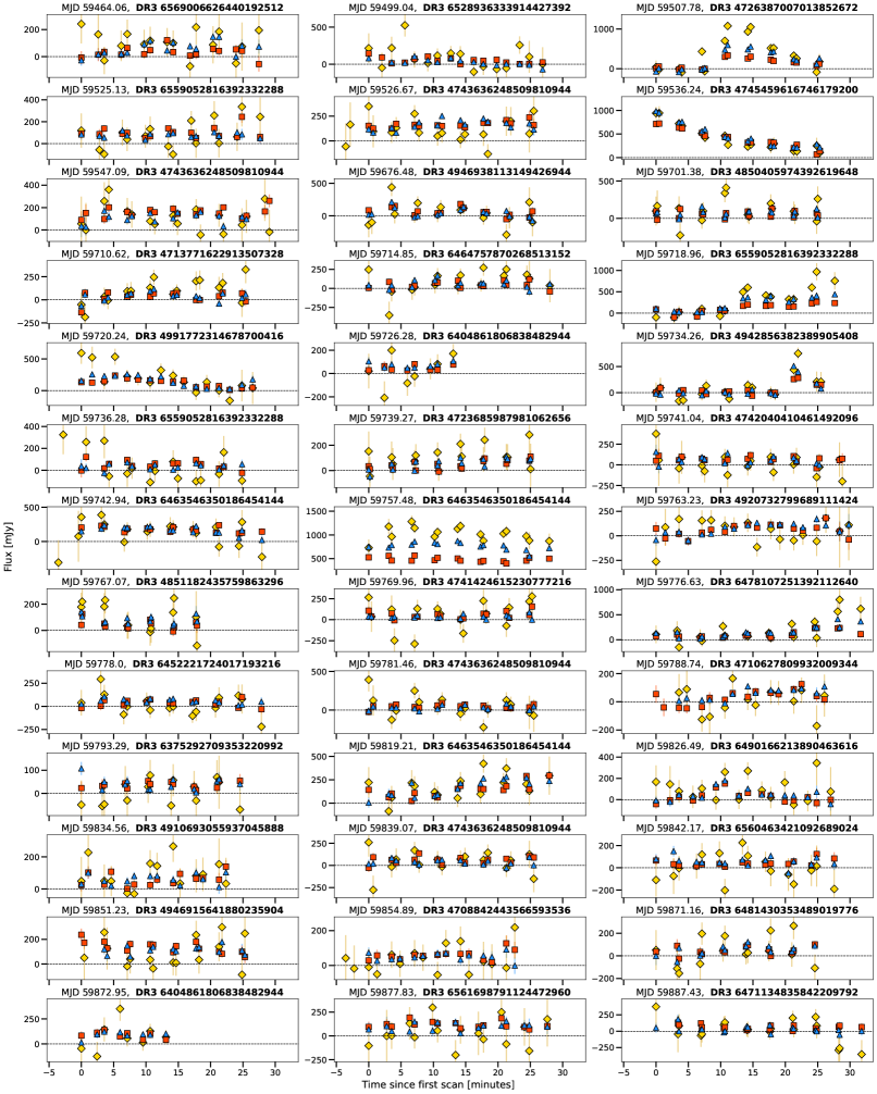
Figure A1: Additional single scan lightcurves.

Table A1: Luminosities and spectral indices for all stars with multiple detected flares.

Gaia DR3 ID	MJD	$\nu L_{\nu,90}$ [erg s-1]	$\nu L_{\nu,150}$ [erg s-1]	$\nu L_{\nu,220}$ [erg s-1]	$\alpha^{90}_{150}$	$\alpha^{150}_{220}$	Flares
6463546350186454144	59757.48	2.19$\times 10^{30}$	5.81$\times 10^{30}$	1.15$\times 10^{31}$	1.14 $\pm$ 0.04	0.78 $\pm$ 0.07	8
	59742.94	8.32$\times 10^{29}$	1.40$\times 10^{30}$	1.93$\times 10^{30}$	0.14 $\pm$ 0.14	-0.17 $\pm$ 0.47
	59819.21	6.34$\times 10^{29}$	1.30$\times 10^{30}$	1.92$\times 10^{30}$	0.58 $\pm$ 0.15	0.0 $\pm$ 0.43
	59003.11	4.00$\times 10^{29}$	8.92$\times 10^{29}$	1.58$\times 10^{30}$	0.76 $\pm$ 0.35	0.49 $\pm$ 1.01
	59096.39	5.42$\times 10^{29}$	7.58$\times 10^{29}$	4.73$\times 10^{29}$	-0.27 $\pm$ 0.21	-2.23 $\pm$ 1.63
	58755.38	4.70$\times 10^{29}$	7.42$\times 10^{29}$	1.31$\times 10^{30}$	0.0 $\pm$ 0.24	0.48 $\pm$ 0.61
	59005.50	2.32$\times 10^{29}$	3.35$\times 10^{29}$	3.15$\times 10^{29}$	-0.2 $\pm$ 0.5	-1.16 $\pm$ 2.39
	59308.02	1.86$\times 10^{29}$	2.64$\times 10^{29}$	3.06$\times 10^{29}$	-0.23 $\pm$ 0.59	-0.61 $\pm$ 2.51
6559052816392332288	59024.26	2.79$\times 10^{30}$	4.54$\times 10^{30}$	6.25$\times 10^{30}$	0.06 $\pm$ 0.04	-0.16 $\pm$ 0.14	6
	59017.39	2.37$\times 10^{30}$	3.84$\times 10^{30}$	6.58$\times 10^{30}$	0.06 $\pm$ 0.04	0.41 $\pm$ 0.13
	59718.96	5.32$\times 10^{29}$	1.62$\times 10^{30}$	2.83$\times 10^{30}$	1.44 $\pm$ 0.16	0.45 $\pm$ 0.28
	59353.05	9.69$\times 10^{29}$	1.18$\times 10^{30}$	7.91$\times 10^{29}$	-0.56 $\pm$ 0.16	-2.06 $\pm$ 1.25
	59525.13	4.01$\times 10^{29}$	5.27$\times 10^{29}$	5.20$\times 10^{29}$	-0.4 $\pm$ 0.3	-1.04 $\pm$ 1.59
	59736.28	2.13$\times 10^{29}$	2.29$\times 10^{29}$	4.68$\times 10^{28}$	-0.84 $\pm$ 0.65	-5.14 $\pm$ 16.47
6478107251392112640	59776.63	6.40$\times 10^{29}$	1.40$\times 10^{30}$	1.81$\times 10^{30}$	0.71 $\pm$ 0.19	-0.33 $\pm$ 0.58	6
	58645.25	6.63$\times 10^{29}$	1.14$\times 10^{30}$	1.51$\times 10^{30}$	0.18 $\pm$ 0.26	-0.26 $\pm$ 0.89
	58941.62	5.74$\times 10^{29}$	1.06$\times 10^{30}$	1.96$\times 10^{30}$	0.34 $\pm$ 0.25	0.61 $\pm$ 0.72
	59382.16	3.80$\times 10^{29}$	5.12$\times 10^{29}$	7.59$\times 10^{29}$	-0.35 $\pm$ 0.42	0.03 $\pm$ 1.49
	58808.69	3.49$\times 10^{29}$	4.57$\times 10^{29}$	3.02$\times 10^{28}$	-0.41 $\pm$ 0.52	-8.1 $\pm$ 38.87
	59346.44	2.55$\times 10^{29}$	2.75$\times 10^{29}$	7.74$\times 10^{28}$	-0.84 $\pm$ 0.69	-4.31 $\pm$ 13.19
6471134835842209792	58961.91	2.24$\times 10^{30}$	4.92$\times 10^{30}$	6.11$\times 10^{30}$	0.73 $\pm$ 0.14	-0.43 $\pm$ 0.41	5
	58655.80	7.54$\times 10^{29}$	1.20$\times 10^{30}$	2.20$\times 10^{30}$	0.02 $\pm$ 0.47	0.59 $\pm$ 1.2
	58966.06	5.51$\times 10^{29}$	8.38$\times 10^{29}$	4.47$\times 10^{29}$	-0.08 $\pm$ 0.71	-2.64 $\pm$ 6.81
	59887.43	7.24$\times 10^{29}$	7.66$\times 10^{29}$	1.45$\times 10^{30}$	-0.88 $\pm$ 0.66	0.66 $\pm$ 2.08
	58591.69	6.20$\times 10^{29}$	6.88$\times 10^{29}$	8.49$\times 10^{28}$	-0.77 $\pm$ 0.76	-6.46 $\pm$ 32.38
4743636248509810944	59526.67	8.00$\times 10^{29}$	1.36$\times 10^{30}$	1.17$\times 10^{30}$	0.15 $\pm$ 0.14	-1.38 $\pm$ 0.7	5
	59547.09	8.03$\times 10^{29}$	8.69$\times 10^{29}$	1.06$\times 10^{30}$	-0.83 $\pm$ 0.19	-0.47 $\pm$ 0.83
	59379.72	2.37$\times 10^{29}$	2.78$\times 10^{29}$	3.38$\times 10^{29}$	-0.65 $\pm$ 0.58	-0.5 $\pm$ 2.97
	59839.07	2.82$\times 10^{29}$	2.61$\times 10^{29}$	6.20$\times 10^{29}$	-1.17 $\pm$ 0.57	1.26 $\pm$ 1.41
	59781.46	2.46$\times 10^{29}$	2.50$\times 10^{29}$	4.74$\times 10^{29}$	-0.97 $\pm$ 0.63	0.67 $\pm$ 1.85
4742040410461492096	58705.72	2.27$\times 10^{28}$	3.87$\times 10^{28}$	8.66$\times 10^{28}$	0.17 $\pm$ 0.22	1.1 $\pm$ 0.46	5
	59373.10	1.64$\times 10^{28}$	3.34$\times 10^{28}$	7.71$\times 10^{28}$	0.56 $\pm$ 0.26	1.18 $\pm$ 0.5
	58719.74	1.03$\times 10^{28}$	2.00$\times 10^{28}$	7.43$\times 10^{28}$	0.44 $\pm$ 0.46	2.43 $\pm$ 0.6
	59741.04	1.37$\times 10^{28}$	1.84$\times 10^{28}$	7.67$\times 10^{27}$	-0.36 $\pm$ 0.44	-3.28 $\pm$ 5.48
	59413.11	6.80$\times 10^{27}$	1.82$\times 10^{28}$	7.61$\times 10^{27}$	1.16 $\pm$ 0.57	-3.28 $\pm$ 4.73
4946938113149426944	59158.65	4.11$\times 10^{27}$	9.07$\times 10^{27}$	1.74$\times 10^{28}$	0.74 $\pm$ 0.08	0.7 $\pm$ 0.19	4
	59109.20	2.44$\times 10^{27}$	7.05$\times 10^{27}$	1.53$\times 10^{28}$	1.32 $\pm$ 0.13	1.02 $\pm$ 0.22
	59040.35	1.01$\times 10^{27}$	1.96$\times 10^{27}$	1.33$\times 10^{27}$	0.44 $\pm$ 0.34	-2.02 $\pm$ 2.06
	59676.48	1.06$\times 10^{27}$	1.43$\times 10^{27}$	1.26$\times 10^{27}$	-0.36 $\pm$ 0.39	-1.34 $\pm$ 2.27
6452221724017193216	59778.00	1.55$\times 10^{29}$	3.64$\times 10^{29}$	5.42$\times 10^{28}$	0.87 $\pm$ 0.45	-5.97 $\pm$ 10.39	3
	58667.89	1.39$\times 10^{29}$	2.92$\times 10^{29}$	4.16$\times 10^{29}$	0.61 $\pm$ 0.51	-0.07 $\pm$ 1.37
	58958.14	1.62$\times 10^{29}$	2.69$\times 10^{29}$	4.46$\times 10^{29}$	0.11 $\pm$ 0.5	0.32 $\pm$ 1.36
4910693055937045888	59834.56	7.41$\times 10^{28}$	1.40$\times 10^{29}$	2.70$\times 10^{29}$	0.39 $\pm$ 0.44	0.72 $\pm$ 0.96	3
	58949.56	5.83$\times 10^{28}$	1.35$\times 10^{29}$	2.93$\times 10^{29}$	0.83 $\pm$ 0.5	1.03 $\pm$ 0.88
	59428.56	7.81$\times 10^{28}$	1.15$\times 10^{29}$	2.90$\times 10^{28}$	-0.15 $\pm$ 0.46	-4.6 $\pm$ 8.6
4723685987981062656	58747.57	7.91$\times 10^{29}$	2.31$\times 10^{30}$	3.20$\times 10^{30}$	1.34 $\pm$ 0.24	-0.14 $\pm$ 0.53	3
	59739.27	4.52$\times 10^{29}$	1.02$\times 10^{30}$	2.96$\times 10^{30}$	0.79 $\pm$ 0.47	1.77 $\pm$ 0.62
	59361.00	3.21$\times 10^{29}$	6.80$\times 10^{29}$	5.93$\times 10^{29}$	0.65 $\pm$ 0.59	-1.36 $\pm$ 2.68
6404861806838482944	59872.95	1.25$\times 10^{30}$	2.50$\times 10^{30}$	2.83$\times 10^{30}$	0.52 $\pm$ 0.32	-0.67 $\pm$ 1.06	2
	59726.28	7.35$\times 10^{29}$	1.87$\times 10^{30}$	2.12$\times 10^{30}$	1.05 $\pm$ 0.52	-0.68 $\pm$ 1.52
6396977135940047616	59338.88	1.80$\times 10^{28}$	2.64$\times 10^{28}$	3.30$\times 10^{28}$	-0.16 $\pm$ 0.33	-0.42 $\pm$ 1.37	2
	59393.69	8.83$\times 10^{27}$	1.85$\times 10^{28}$	4.51$\times 10^{28}$	0.62 $\pm$ 0.55	1.33 $\pm$ 0.96
4979859106192681344	58594.72	3.44$\times 10^{28}$	7.56$\times 10^{28}$	1.27$\times 10^{29}$	0.72 $\pm$ 0.56	0.35 $\pm$ 1.42	2
	58808.36	2.93$\times 10^{28}$	7.16$\times 10^{28}$	5.35$\times 10^{27}$	0.96 $\pm$ 0.63	-7.78 $\pm$ 30.45
4928347433108236416	59447.56	5.48$\times 10^{27}$	1.35$\times 10^{28}$	2.26$\times 10^{28}$	0.97 $\pm$ 0.39	0.36 $\pm$ 0.85	2
	58590.05	5.00$\times 10^{27}$	7.40$\times 10^{27}$	1.30$\times 10^{28}$	-0.14 $\pm$ 0.63	0.46 $\pm$ 1.94
4726387007013852672	59507.78	5.84$\times 10^{27}$	1.67$\times 10^{28}$	4.38$\times 10^{28}$	1.3 $\pm$ 0.09	1.52 $\pm$ 0.13	2
	58982.09	1.35$\times 10^{27}$	2.37$\times 10^{27}$	1.47$\times 10^{27}$	0.23 $\pm$ 0.49	-2.26 $\pm$ 3.39
4713771622913507328	58798.28	1.02$\times 10^{28}$	1.57$\times 10^{28}$	1.88$\times 10^{28}$	-0.06 $\pm$ 0.21	-0.53 $\pm$ 0.79	2
	59710.62	3.84$\times 10^{27}$	7.03$\times 10^{27}$	2.15$\times 10^{28}$	0.32 $\pm$ 0.49	1.92 $\pm$ 0.72
4708842443566593536	59345.82	1.72$\times 10^{30}$	5.16$\times 10^{30}$	1.03$\times 10^{31}$	1.4 $\pm$ 0.18	0.8 $\pm$ 0.32	2
	59854.89	1.25$\times 10^{30}$	1.71$\times 10^{30}$	1.74$\times 10^{30}$	-0.32 $\pm$ 0.39	-0.96 $\pm$ 1.7

References

- Abazajian et al. (2019) Abazajian, K., Addison, G., Adshead, P., et al. 2019, arXiv e-prints, arXiv:1907.04473
- Ade et al. (2019) Ade, P., Aguirre, J., Ahmed, Z., et al. 2019, Journal of Cosmology and Astroparticle Physics, 2019, 056
- Allred et al. (2015) Allred, J. C., Kowalski, A. F., & Carlsson, M. 2015, ApJ, 809, 104
- Anfinogentov et al. (2013) Anfinogentov, S., Nakariakov, V. M., Mathioudakis, M., Van Doorsselaere, T., & Kowalski, A. F. 2013, ApJ, 773, 156
- Aschwanden et al. (2008) Aschwanden, M. J., Stern, R. A., & Güdel, M. 2008, ApJ, 672, 659
- Audard et al. (2000) Audard, M., Güdel, M., Drake, J. J., & Kashyap, V. L. 2000, ApJ, 541, 396
- Balona (2012) Balona, L. A. 2012, MNRAS, 423, 3420
- Balona (2015) —. 2015, MNRAS, 447, 2714
- Bastian et al. (1998) Bastian, T. S., Benz, A. O., & Gary, D. E. 1998, ARA&A, 36, 131
- Beasley & Bastian (1998) Beasley, A. J., & Bastian, T. S. 1998, in Astronomical Society of the Pacific Conference Series, Vol. 144, IAU Colloq. 164: Radio Emission from Galactic and Extragalactic Compact Sources, ed. J. A. Zensus, G. B. Taylor, & J. M. Wrobel, 321
- Bell et al. (2015) Bell, C. P. M., Mamajek, E. E., & Naylor, T. 2015, MNRAS, 454, 593
- Benz (2017) Benz, A. O. 2017, Living Reviews in Solar Physics, 14, 2
- Benz & Güdel (2010) Benz, A. O., & Güdel, M. 2010, ARA&A, 48, 241
- Bochanski et al. (2010) Bochanski, J. J., Hawley, S. L., Covey, K. R., et al. 2010, The Astronomical Journal, 139, 2679
- Boller et al. (2016) Boller, T., Freyberg, M. J., Trümper, J., et al. 2016, A&A, 588, A103
- Brasseur et al. (2019) Brasseur, C. E., Osten, R. A., & Fleming, S. W. 2019, ApJ, 883, 88
- Braun et al. (2010) Braun, J., Baker, M., Dumm, J., et al. 2010, Astroparticle Physics, 33, 175
- Brown (1971) Brown, J. C. 1971, Sol. Phys., 18, 489
- Brown & Brown (2006) Brown, J. M., & Brown, A. 2006, ApJ, 638, L37
- Burton et al. (2022) Burton, K., MacGregor, M. A., & Osten, R. A. 2022, ApJ, 939, L6
- Carlstrom et al. (2011) Carlstrom, J. E., Ade, P. A. R., Aird, K. A., et al. 2011, Publications of the Astronomical Society of the Pacific, 123, 568
- Catalano (1986) Catalano, S. 1986, Rutherford Appleton Laboratory Report, 85, 105
- Davenport (2016) Davenport, J. R. A. 2016, ApJ, 829, 23
- Davenport et al. (2012) Davenport, J. R. A., Becker, A. C., Kowalski, A. F., et al. 2012, ApJ, 748, 58
- Davenport et al. (2014) Davenport, J. R. A., Hawley, S. L., Hebb, L., et al. 2014, ApJ, 797, 122
- Dutcher et al. (2021) Dutcher, D., Balkenhol, L., Ade, P. A. R., et al. 2021, Phys. Rev. D, 104, 022003
- Eftekhari et al. (2022) Eftekhari, T., Berger, E., Metzger, B. D., et al. 2022, ApJ, 935, 16
- Feigelson & Montmerle (1999) Feigelson, E. D., & Montmerle, T. 1999, ARA&A, 37, 363
- Finch et al. (2014) Finch, C. T., Zacharias, N., Subasavage, J. P., Henry, T. J., & Riedel, A. R. 2014, AJ, 148, 119
- Fletcher et al. (2011) Fletcher, L., Dennis, B. R., Hudson, H. S., et al. 2011, Space Sci. Rev., 159, 19
- France et al. (2016) France, K., Loyd, R. O. P., Youngblood, A., et al. 2016, ApJ, 820, 89
- Freund et al. (2022) Freund, S., Czesla, S., Robrade, J., Schneider, P. C., & Schmitt, J. H. M. M. 2022, A&A, 664, A105
- Galassi et al. (2009) Galassi, M., Davies, J., Theiler, J., Gough, B., & Jungman, G. 2009, GNU Scientific Library - Reference Manual, Third Edition, for GSL Version 1.12 (3. ed.).
- Getman & Feigelson (2021) Getman, K. V., & Feigelson, E. D. 2021, ApJ, 916, 32
- Güdel (2004) Güdel, M. 2004, A&A Rev., 12, 71
- Guns et al. (2021) Guns, S., Foster, A., Daley, C., et al. 2021, ApJ, 916, 98
- Günther et al. (2020) Günther, M. N., Zhan, Z., Seager, S., et al. 2020, AJ, 159, 60
- Henry & Newsom (1996) Henry, G. W., & Newsom, M. S. 1996, PASP, 108, 242
- Howard & MacGregor (2022) Howard, W. S., & MacGregor, M. A. 2022, ApJ, 926, 204
- Hudson (1972) Hudson, H. S. 1972, Sol. Phys., 24, 414
- Hunter (2007) Hunter, J. D. 2007, Computing In Science & Engineering, 9, 90
- Jones et al. (2001) Jones, E., Oliphant, T., Peterson, P., et al. 2001, SciPy: Open source scientific tools for Python, [Online; accessed 2014-10-22]
- Koch et al. (2010) Koch, D. G., Borucki, W. J., Basri, G., et al. 2010, ApJ, 713, L79
- Kowalski et al. (2019) Kowalski, A. F., Wisniewski, J. P., Hawley, S. L., et al. 2019, ApJ, 871, 167
- Krucker et al. (2013) Krucker, S., Giménez de Castro, C. G., Hudson, H. S., et al. 2013, A&A Rev., 21, 58
- Krucker et al. (2015) Krucker, S., Saint-Hilaire, P., Hudson, H. S., et al. 2015, ApJ, 802, 19
- Kundu & Vlahos (1982) Kundu, M. R., & Vlahos, L. 1982, Space Sci. Rev., 32, 405
- Lang (2014) Lang, D. 2014, AJ, 147, 108
- Large et al. (1989) Large, M. I., Beasley, A. J., Stewart, R. T., & Vaughan, A. E. 1989, PASA, 8, 123
- Levinson et al. (2002) Levinson, A., Ofek, E. O., Waxman, E., & Gal-Yam, A. 2002, ApJ, 576, 923
- Li et al. (2023) Li, Y., Biermann, E., Naess, S., et al. 2023, The Astrophysical Journal, 956, 36
- Loyd et al. (2018a) Loyd, R. O. P., France, K., Youngblood, A., et al. 2018a, ApJ, 867, 71
- Loyd et al. (2018b) —. 2018b, ApJ, 867, 71
- Lüthi et al. (2004) Lüthi, T., Magun, A., & Miller, M. 2004, A&A, 415, 1123
- MacGregor et al. (2020) MacGregor, A. M., Osten, R. A., & Hughes, A. M. 2020, ApJ, 891, 80
- MacGregor et al. (2018) MacGregor, M. A., Weinberger, A. J., Wilner, D. J., Kowalski, A. F., & Cranmer, S. R. 2018, ApJ, 855, L2
- MacGregor et al. (2021) MacGregor, M. A., Weinberger, A. J., Loyd, R. O. P., et al. 2021, ApJ, 911, L25
- Mairs et al. (2019) Mairs, S., Lalchand, B., Bower, G. C., et al. 2019, ApJ, 871, 72
- Massi et al. (2006) Massi, M., Forbrich, J., Menten, K. M., et al. 2006, A&A, 453, 959
- Massi et al. (2002) Massi, M., Menten, K., & Neidhöfer, J. 2002, A&A, 382, 152
- Murphy et al. (2013) Murphy, T., Chatterjee, S., Kaplan, D. L., et al. 2013, PASA, 30, e006
- Naess et al. (2021) Naess, S., Battaglia, N., Richard Bond, J., et al. 2021, ApJ, 915, 14
- Ochsenbein et al. (2000) Ochsenbein, F., Bauer, P., & Marcout, J. 2000, A&AS, 143, 23
- Osten & Brown (1999) Osten, R. A., & Brown, A. 1999, ApJ, 515, 746
- Pacholczyk (1970) Pacholczyk, A. G. 1970, Radio astrophysics. Nonthermal processes in galactic and extragalactic sources
- Pearce & Harrison (1990) Pearce, G., & Harrison, R. A. 1990, A&A, 228, 513
- Pettersen (1989) Pettersen, B. R. 1989, Sol. Phys., 121, 299
- Pevtsov et al. (2003) Pevtsov, A. A., Fisher, G. H., Acton, L. W., et al. 2003, ApJ, 598, 1387
- Pordes et al. (2007) Pordes, R., et al. 2007, J. Phys. Conf. Ser., 78, 012057
- Pye et al. (2015) Pye, J. P., Rosen, S., Fyfe, D., & Schröder, A. C. 2015, A&A, 581, A28
- Raulin et al. (1999) Raulin, J.-P., White, S., Kundu, M., Valio, A., & Shibasaki, K. 1999, The Astrophysical Journal, 522
- Reiners et al. (2010) Reiners, A., Seifahrt, A., & Dreizler, S. 2010, A&A, 513, L9
- Reinhold et al. (2020) Reinhold, T., Shapiro, A. I., Solanki, S. K., et al. 2020, Science, 368, 518
- Ricker et al. (2014) Ricker, G. R., Winn, J. N., Vanderspek, R., et al. 2014, in Society of Photo-Optical Instrumentation Engineers (SPIE) Conference Series, Vol. 9143, Space Telescopes and Instrumentation 2014: Optical, Infrared, and Millimeter Wave, ed. J. Oschmann, Jacobus M., M. Clampin, G. G. Fazio, & H. A. MacEwen, 914320
- Riedel et al. (2014) Riedel, A. R., Finch, C. T., Henry, T. J., et al. 2014, AJ, 147, 85
- Rimoldini et al. (2023) Rimoldini, L., Holl, B., Gavras, P., et al. 2023, A&A, 674, A14
- Schaefer et al. (2000) Schaefer, B. E., King, J. R., & Deliyannis, C. P. 2000, ApJ, 529, 1026
- Schmitt et al. (1995) Schmitt, J. H. M. M., Fleming, T. A., & Giampapa, M. S. 1995, ApJ, 450, 392
- Sfiligoi et al. (2009) Sfiligoi, I., Bradley, D. C., Holzman, B., et al. 2009, in 2, Vol. 2, 2009 WRI World Congress on Computer Science and Information Engineering, 428
- Shields et al. (2016) Shields, A. L., Ballard, S., & Johnson, J. A. 2016, Phys. Rep., 663, 1
- Silva et al. (1996) Silva, A. V. R., White, S. M., Lin, R. P., et al. 1996, ApJ, 458, L49
- Smith et al. (2005) Smith, K., Güdel, M., & Audard, M. 2005, A&A, 436, 241
- Sobrin et al. (2022) Sobrin, J. A., Anderson, A. J., Bender, A. N., et al. 2022, ApJS, 258, 42
- Stassun et al. (2019) Stassun, K. G., Oelkers, R. J., Paegert, M., et al. 2019, AJ, 158, 138
- Umemoto et al. (2009) Umemoto, T., Saito, M., Nakanishi, K., Kuno, N., & Tsuboi, M. 2009, Astronomical Society of the Pacific Conference Series, Vol. 402, ed. Y. Hagiwara, E. Fomalont, M. Tsuboi, and M. Yasuhiro, 400
- van der Walt et al. (2011) van der Walt, S., Colbert, S., & Varoquaux, G. 2011, Computing in Science Engineering, 13, 22
- Van Doorsselaere et al. (2017) Van Doorsselaere, T., Shariati, H., & Debosscher, J. 2017, ApJS, 232, 26
- van Leeuwen (2007) van Leeuwen, F. 2007, A&A, 474, 653
- van Leeuwen et al. (2022) van Leeuwen, F., de Bruijne, J., Babusiaux, C., et al. 2022, Gaia DR3 documentation
- Webber et al. (1973) Webber, J. C., Yoss, K. M., Deming, D., Yang, K. S., & Green, R. F. 1973, PASP, 85, 739
- Whitehorn et al. (2016) Whitehorn, N., Natoli, T., Ade, P. A. R., et al. 2016, The Astrophysical Journal, 830, 143
- Yang et al. (2017) Yang, H., Liu, J., Gao, Q., et al. 2017, ApJ, 849, 36
- Zhang et al. (2018) Zhang, P., Guo, Y., Wang, L., & Liu, S. 2018, A&A, 615, A48
- Zhou et al. (2011) Zhou, A. H., Li, J. P., & Wang, X. D. 2011, ApJ, 727, 42