Separable Physics-Informed Neural Networks for the Solution of Elasticity Problems

Abstract

A method for solving elasticity problems based on separable physics-informed neural networks (SPINN) in conjunction with the deep energy method (DEM) is presented. Numerical experiments have been carried out for a number of problems showing that this method has a significantly higher convergence rate and accuracy than the vanilla physics-informed neural networks (PINN) and even SPINN based on a system of partial differential equations (PDEs). In addition, using the SPINN in the framework of DEM approach it is possible to solve problems of the linear theory of elasticity on complex geometries, which is unachievable with the help of PINNs in frames of partial differential equations. Considered problems are very close to the industrial problems in terms of geometry, loading, and material parameters.

Keywords Deep Learning  $\cdot$ Physics-informed Neural Networks  $\cdot$ Partial differential equations  $\cdot$ Predictive modeling  $\cdot$ Computational physics

1 Introduction

The recent few years have been marked by revolutionary achievements in the field of machine learning referred to Deep Neural Networks (DNN) and Deep Learning (DL) [1]. Continued improvement of DNN architecture and refinement of the training methods have led to the various applications which possess the capabilities previously available only for humans [2, 3, 4]. Neural networks based approaches are widely spread in image classification, handwriting recognition, speech recognition, and translation, text generators, game systems and computer vision [5, 6, 7, 8, 9, 10, 11, 12]. This revolutionary transformation and the implementation of deep learning achievements in many areas of professional activity has not left aside the scientific and engineering fields. Developed DNN systems for solving scientific and engineering problems can be separated into those that leverage previously established physical laws (PINN) [13, 14, 15, 16, 17], those that utilized previously obtained data (from computations or experiments) and build their predictions on this basis [18, 19, 20, 21, 22, 23], and those that exploit both these approaches [24, 25, 26]. In our paper we exclusively focus on PINN methods, avoiding data-driven approaches.

The main ideas for the training of neural networks, which predict the physical system behaviour, using physical laws have been around for decades[27, 28]. Due to modern computational tools, these ideas incarnated a few years ago in new approaches, such as (PINN) [13]. The neural networks of these methods are trained to approximate the dependences of physical values with the help of equations together with initial and boundary conditions. This approach has been used to solve a wide range of problems described by ordinary differential equations [24, 25, 13, 29], integro-differential equations [30], nonlinear partial differential equations [24, 25, 13, 31, 32, 33], PDE with noisy data [34], etc. [35, 36], related to various fields of knowledge such as thermodynamics [37, 38], hydrodynamics [39, 31, 32], electrodynamics [40, 33], geophysics [41], finance [30], mechanics [42, 43, 44, 45, 46, 47, 48] and thermo-mechanically coupled systems [49].

Despite the PINN success in solid mechanics [42, 43, 44, 45, 46], for the 3D elasticity problem under complex geometry the PINN based only partial differential equations, which described displacements and stresses demonstrates low convergence. To address this drawback differential equations can be used along with conservation laws [15] in the PINN approach, or only the energy conservation law [44, 48], which result in accuracy improvement for the considered problems. Another concern of the PINN is the low speed of training (but high speed of the evaluation) which can be solved by novel types of neural networks such as separable physics-informed neural networks (SPINN) [50]. The training time of SPINN is comparable with the time of obtaining an acceptable solution with the help of classical numerical methods like the finite element method (FEM).

This work is devoted to the application of a number of techniques that can improve the accuracy of prediction and the speed of training and evaluation on the basis of the PINN approach for the 3D elasticity problems. We will briefly list the contributions made in the paper. We will briefly list the contributions made in the paper:

1. The method for solving elasticity problems based on separable physics-informed neural networks in conjunction with the deep energy method is proposed.

2. A comparison of the speed and accuracy of training for different PINNs is carried out: PINN based on PDE, SPINN based on PDE, SPINN based on a minimum of energy.

3. It demonstrates that SPINN in the framework DEM approach solves problems of the linear elasticity on complex geometries, which is unachievable with PINNs in terms of partial differential equations.

The paper is structured as follows. In section 2, the statement of the problem of linear elasticity on the basis of both the partial differential equation and energy minimization is presented. Section 3 includes the description of PINN approach for two different statements of the problem. Descriptions of architectures of the artificial neural networks, that were used in the work, are also provided here. In Section 4, numerical experiments to illustrate the accuracy and efficiency of the presented approach are given. Finally, in Section 5 concluding remarks are given.

2 Statement of the Problem

2.1 Formulation of the problem on the basis of partial differential equations

Consider a deformed body in a state of static equilibrium under the effect of external volumetric force ${\bf f}$ and external force on unit area of surface ${\bf T}$. Such an object is described by the following system of partial differential equations (PDE) [51]

$$\frac{\partial\sigma_{ik}}{\partial x_{k}}+f_{i}=0,\,\quad{\bf x}\in\Omega.$$ (1)

and boundary conditions

$$\sigma_{ik}n_{k}=T_{i},\quad{\bf x}\in\partial\Omega,$$ (2)

$${\bf u}={\bf u}^{(b)},\quad{\bf x}\in\partial\Omega.$$ (3)

Here, ${\bf x}$ are spatial coordinates, $\sigma_{ik}$ is the stress tensor, ${\bf n}$ is a unit vector along the outward normal to the surface, ${\bf u}$ is displacement vector, ${\bf u}^{(b)}$ is displacement vector at boundaries, $\Omega$ and $\partial\Omega$ are the spatial domain of body and its boundary, respectively. The conditions (2) and (3) must be satisfied at every point of the surface of a body in equilibrium. Here and further, Einstein summation notation is used which dictates repeated indices should be summed.

The stress tensor is given in terms of the strain tensor by Hook law

$$\sigma_{ik}=\lambda\varepsilon_{ll}\delta_{ik}+\mu\varepsilon_{ik},$$ (4)

where the strain tensor $\varepsilon_{ik}$ is

$$\varepsilon_{ik}=\frac{1}{2}\left(\frac{\partial u_{i}}{\partial x_{k}}+\frac{\partial u_{k}}{\partial x_{i}}\right),$$ (5)

the coefficients (Lame constants) are

$$\lambda=\frac{\nu E}{2(1+\nu)(1-2\nu)},\quad\mu=\frac{E}{2(1+\nu)},$$ (6)

$\delta_{ik}$ is Kronecker symbol, $E$ and $\nu$ are Young’s modulus and Poisson’s ratio, respectively.

In all examples, we assume volumetric force is the gravitation force ${\bf f}=\rho{\bf g}$; $\rho$ is the density of body material and ${\bf g}$ is the gravitational acceleration vector.

In the Cartesian coordinate system ($x,y,z$) the system of equations (1) has the following form

$$\frac{\partial\sigma_{xx}}{\partial x}+\frac{\partial\sigma_{xy}}{\partial y}+\frac{\partial\sigma_{xz}}{\partial z}=0,$$ (7)

$$\frac{\partial\sigma_{xy}}{\partial x}+\frac{\partial\sigma_{yy}}{\partial y}+\frac{\partial\sigma_{yz}}{\partial z}=0,$$ (8)

$$\frac{\partial\sigma_{xz}}{\partial x}+\frac{\partial\sigma_{yz}}{\partial y}+\frac{\partial\sigma_{zz}}{\partial z}-\rho g=0.$$ (9)

The axes of a given Cartesian coordinate system are oriented so that the vector ${\bf g}$ is directed in the negative direction of $z$–axis. Here, the symmetrical properties of the stress tensor ($\sigma_{ik}=\sigma_{ki}$) are used.

Equations (1) together with boundary conditions (2) and (3) are the total description of the steady-state linear elasticity problem which has a unique solution. This problem can be solved by using the classical finite-element method (FEM) or by a novel physics-informed neural network approach (PINN) [24, 25, 13].

2.2 Formulation of the problem on the basis of energy minimization

Instead of the PDE (1) with boundary conditions (2) and (3) the steady-state linear elasticity problem can be considered in the following energy approach [51, 44]

$${\bf{u}}^{*}=\underset{\bf{u}}{\arg}\min\mathcal{E}(\bf{u}),$$ (10)

where ${\bf u}^{*}$ is the solution of the problem (1)–(3), $\mathcal{E}$ is the total energy of system which is defined as

$$\mathcal{E}\left({\bf u}\right)=\frac{1}{2}\int_{\Omega}\left(\sigma_{ik}\varepsilon_{ik}\right)dV-\int_{\Omega}\left({\bf f}\cdot{\bf u}\right)dV-\oint_{\partial\Omega}\left({\bf T}\cdot{\bf u}\right)dS.$$ (11)

Here $({\bf a}\cdot{\bf b})$ means dot product of two vector ${\bf a}$ and ${\bf b}$, ${\bf u}$ is constrained by boundary conditions (3) for the displacements.

We will assume the displacements for the minimum of the total energy of the system coincide with displacements which are solutions of the problem described by Eqs. (1)–(3).

3 Methods

3.1 Physical-Informed approach

3.1.1 Vanilla PINN

According to the physics-informed neural network (PINN) approach [13], which stands on the shoulders of the universal approximation theorem [52], the PINN approximates the unknown solution ${\bf u}({\bf x})$ of the problem (1)–(3) by a deep neural network ${\bf u}^{{\bm{\theta}}}({\bf x})$, where ${\bm{\theta}}$ denote all trainable parameters of the network (weights and biases). Finding optimal parameters is an optimization problem, which requires the definition of a loss function such that its minimum gives the solution of the PDE. The physics-informed model is trained by minimizing the composite loss function which consists of the local residuals of the differential equations (1) over the problem domain and its boundary as shown below:

$$\mathcal{L}({\bm{\theta}})=\lambda_{bc}\mathcal{L}_{bc}({\bm{\theta}})+\mathcal{L}_{r}({\bm{\theta}}),$$ (12)

where

$$\mathcal{L}_{bc}\left(\bm{\theta}\right)=\frac{1}{N_{bc}}\sum_{i=1}^{N_{bc}}\sum_{l=1}^{N_{l}}\left|\mathcal{B}_{l}\left[{\bf u}^{{\bm{\theta}}}\right]\left({\bf x}_{i}^{(bc)}\right)\right|^{2},$$ (13)

$$\mathcal{L}_{r}\left(\bm{\theta}\right)=\frac{1}{N_{r}}\sum_{i=1}^{N_{r}}\sum_{l=1}^{3}\left|\mathcal{R}_{l}\left[{\bf u}^{{\bm{\theta}}}\right]\left({\bf x}_{i}^{(r)}\right)\right|^{2},$$ (14)

$$\mathcal{B}_{l}[{\bf u}]:={u}_{l}-{u}^{(bc)}_{l}\quad\text{or}\quad\mathcal{B}_{l}[{\bf u}]:=\sigma_{lk}n_{k}-T_{l},$$ (15)

$$\mathcal{R}_{l}\left[{\bf u}\right]:=\frac{\partial\sigma_{lk}}{\partial x_{k}}+f_{l}.$$ (16)

Here $\left\{{\bf x}_{i}^{(bc)}\right\}^{N_{bc}}_{i=1}$ and $\left\{{\bf x}_{i}^{(r)}\right\}^{N_{r}}_{i=1}$ are sets of points corresponding to boundary condition domain and PDE domain, respectively. These points can be the vertices of a fixed mesh or can be randomly sampled at each iteration of a gradient descent algorithm. $\mathcal{B}_{l}$ is a boundary operator corresponding to $l$th boundary conditions at the given boundary point, $\mathcal{R}_{l}$ is a residual operator which is determined by the $l$th equation of PDEs (1).

All required gradients, derivations (for example, $\sigma_{lk}$ and $\partial\sigma_{lk}/\partial x_{k}$) w.r.t. input variables ($\bf x$) and network parameters $\theta$ can be efficiently computed via automatic differentiation [53] with algorithmic accuracy, which is defined by the accuracy of computation system. The hyperparameter $\lambda_{bc}$ allows for separate tuning of the learning rate for each of the loss terms in order to improve the convergence of the model [54, 55].

The optimization problem can be defined as follows

$${\bm{\theta}}^{*}=\underset{{\bm{\theta}}}{\arg}\min\mathcal{L}({\bm{\theta}}),$$ (17)

where ${\bm{\theta}}^{*}$ are optimal parameters of the neural network which minimize the discrepancy between the exact unknown solution ${\bf u}$ and the approximate one ${\bf u}_{\boldsymbol{\theta}^{*}}$.

3.1.2 Energy PINN

Following the deep energy method (DEM) [44] the energy of deformation of the mechanical system (11) can be used as the energy term of the loss function (12) instead of residual loss term $\mathcal{L}_{r}(\bm{\theta})$. Then, the following form for the loss function is obtained

$$\mathcal{L}({\bm{\theta}})=\lambda_{bc}\mathcal{L}_{bc}({\bm{\theta}})+\mathcal{L}_{en}({\bm{\theta}}),$$ (18)

where

$$\mathcal{L}_{en}({\bm{\theta}}) =\frac{1}{2}\sum_{i=1}^{N_{en}}w_{i}\left(\sigma_{lk}\left({\bf x}_{i}^{(en)}\right)\varepsilon_{lk}\left({\bf x}_{i}^{(en)}\right)\right)\Delta V_{i}$$

$$-\sum_{i=1}^{N_{en}}w_{i}\left({\bf f}\cdot{{\bf u}^{{\bm{\theta}}}(x_{i})}\right)\Delta V_{i}-\sum_{i=1}^{N_{bc}}w_{i}\left({\bf T}\cdot{\bf u}_{\bm{\theta}}\left({\bf x}_{i}^{(bc)}\right)\right)\Delta S_{i}.$$ (19)

Here $\left\{{\bf x}_{i}^{(en)}\right\}^{N_{en}}_{i=1}$ are set of points corresponding to the domain of body are taken for the integration, $\Delta V_{i}$ is the volume of $i$th cell of the body, $\Delta S_{i}$ is square of $i$th cell of the surface of the body, $w_{i}$ is the weight coefficient of given integration scheme in $i$th point (in our calculations we taken the Simpson’s rule of integration).

Note, in this case of the loss function, the term $\mathcal{L}_{bc}$ is generated by the elements corresponding to boundary conditions (3), but is not for (2) because last conditions are involved in the loss term (19) as an energy of external forces.
The optimization problem is still given by the Eq. (17).

3.2 Artificial Neural Network Architectures

A generic deep neural network with $L$ layers, can be expressed by the composition of $L$ functions $f_{i}({\bf z}_{i};{\bm{\theta}}_{i})$ [56, 35] (where ${\bf z}_{i}$ are the state variables, and ${\bm{\theta}}_{i}$ is the set of parameters of the $i$th layer). The function of interest ${\bf u}_{\bm{\theta}}$ can be represented in the following form

$${\bf u}_{\bm{\theta}}({\bf x})=f_{L}\circ f_{L-1}\circ\dots\circ f_{1}({\bf x}),$$ (20)

where functions $f_{i}$ are determined with inner product of two spaces $E_{i}$ and $H_{i}$, so that $f_{i}\in E_{i}\times H_{i}$; $\circ$ is operator of function composition which reads for function $f_{1}$ and $f_{2}$ as $f_{2}\circ f_{1}({\bf x})=f_{2}\left(f_{1}({\bf x})\right)$.

3.2.1 Multi-layer perceptron

As in the original vanilla PINN [24, 25], the feed-forward neural networks (multi-layer perceptron (MLP)) play the key role in the representation of the solutions for the problems in our paper. This neural network is a set of neurons collected in layers which execute calculations sequentially, layer by layer. Data flow through the MLP in a forward direction without loopback. The neurons of feed-forward neural networks in neighboring layers are connected, whereas neurons of a single layer are not directly related. Every neuron is a collection of sequence mathematical operations which are the sum of weighted neuron’s inputs and a bias factor, and appliance an activation function to the result. The action of one layer of the MLP can be written as

$$f_{i}({\bf z}_{i};{\bf W}_{i},{\bf b}_{i})=\alpha_{i}\left({\bf W}_{i}\cdot{\bf z}_{i}+{\bf b}_{i}\right),$$ (21)

where $z_{i}$ is output of th $(i-1)$th layer, ${\bf W}_{i}$ and ${\bf b}_{i}$ are the the weight and the bias of $i$th layer, respectively, $\alpha_{i}$ is a non-linear activation function. The general representation (20) of artificial neural network for the MLP with identical activation function for all layers can also be rewritten in conformity with the notation [57]

$${\bf u}_{\bm{\theta}}({\bf x})=C_{L}\circ\alpha\circ C_{L-1}\circ\dots\circ\alpha\circ C_{1}({\bf x}),$$ (22)

where for any $k\in[1,2,\cdot,L]$ the $C_{k}$ is defined with

$$C_{k}({\bf x}_{k})={\bf W}_{k}{\bf x}_{k}+{\bf b}_{k}.$$ (23)

Thus this MLP consists of input and output layers, and $(L-2)$ hidden layers.

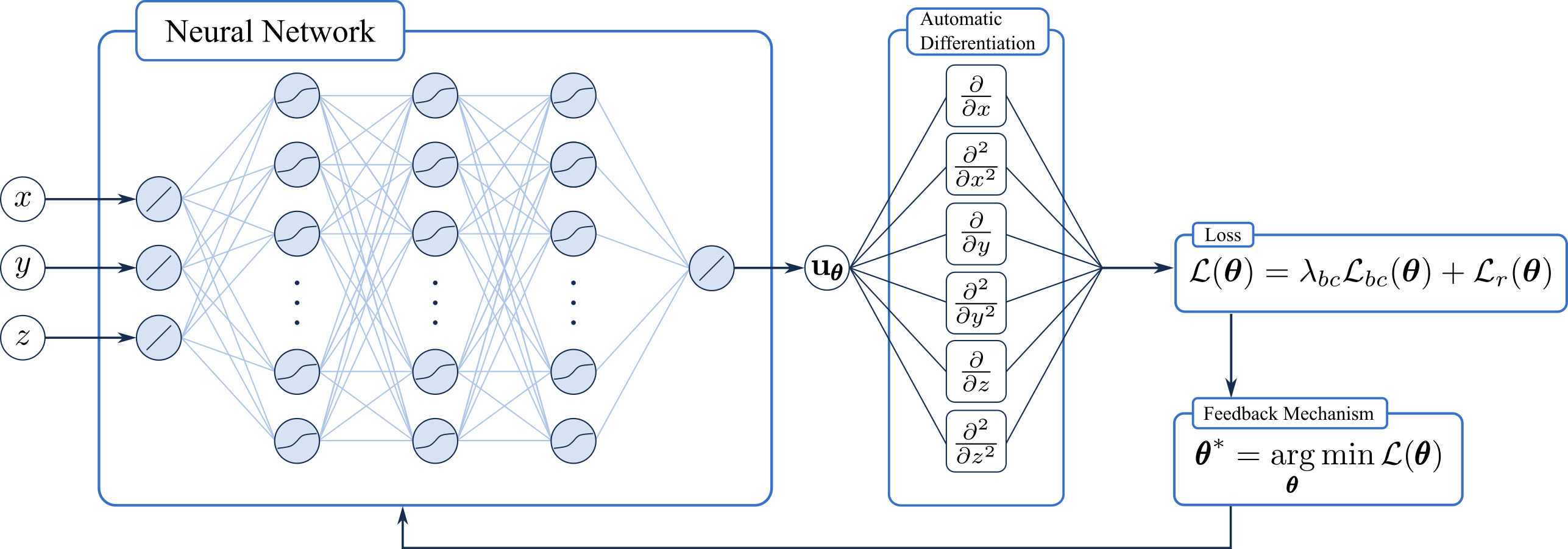
Figure 1: Schematic diagram of the general PINN method.

3.2.2 Separable PINN

In most part of our experiments, we used a novel network architecture, called separable PINN (SPINN), which facilitates significant forward-mode automatic differentiation (AD) for more efficient computation [50]. The brilliant idea behind this approach is using the classic separation of variables method (the Fourier method) for the special representation of the neural network. SPINN uses a per-axis basis instead of point-wise processing in vanilla PINNs, which decreases the number of network forward passes. In addition, training time, evaluating time and memory costs are significantly reduced for the SPINN in comparison to PINN, for which these parameters are grown exponentially along with the grid resolution increasing.

SPINN consists of $d$ body-networks (which are usually presented by MLPs), each of which takes an individual one-dimensional coordinate component as an input from $d$-dimensional space. Each body-network ${\bf f}_{{\bm{\theta}}_{i}}:\mathbb{R}\rightarrow\mathbb{R}^{r}$ (parameterized by ${{\bm{\theta}}_{i}}$) is a vector-valued function which transforms the coordinates of $i$th axis into a $r$-dimensional feature representation (functional basis, or set of eigenfunctions).

The predictions of SPINN are computed by basis functions merging which is defined by following

$${u}^{{\bm{\theta}}}({\bf x})=\sum\limits_{j=1}^{r}\prod\limits_{i=1}^{d}{f}^{{\bm{\theta}}_{i}}_{j}(x_{i}),$$ (24)

where ${u}^{{\bm{\theta}}}:\mathbb{R}^{d}\rightarrow\mathbb{R}$ is the predicted solution function, $x_{i}\in\mathbb{R}$ is coordinate of $i$th axis, and ${f}^{{\bm{\theta}}_{i}}_{j}$ is the $j$th element of basis ${\bf f}^{{\bm{\theta}}_{i}}$ $\left({\bf f}^{{\bm{\theta}}_{i}}=\left({f}^{{\bm{\theta}}_{i}}_{1},{f}^{{\bm{\theta}}_{i}}_{2},\dots,{f}^{{\bm{\theta}}_{i}}_{r}\right)\right)$.

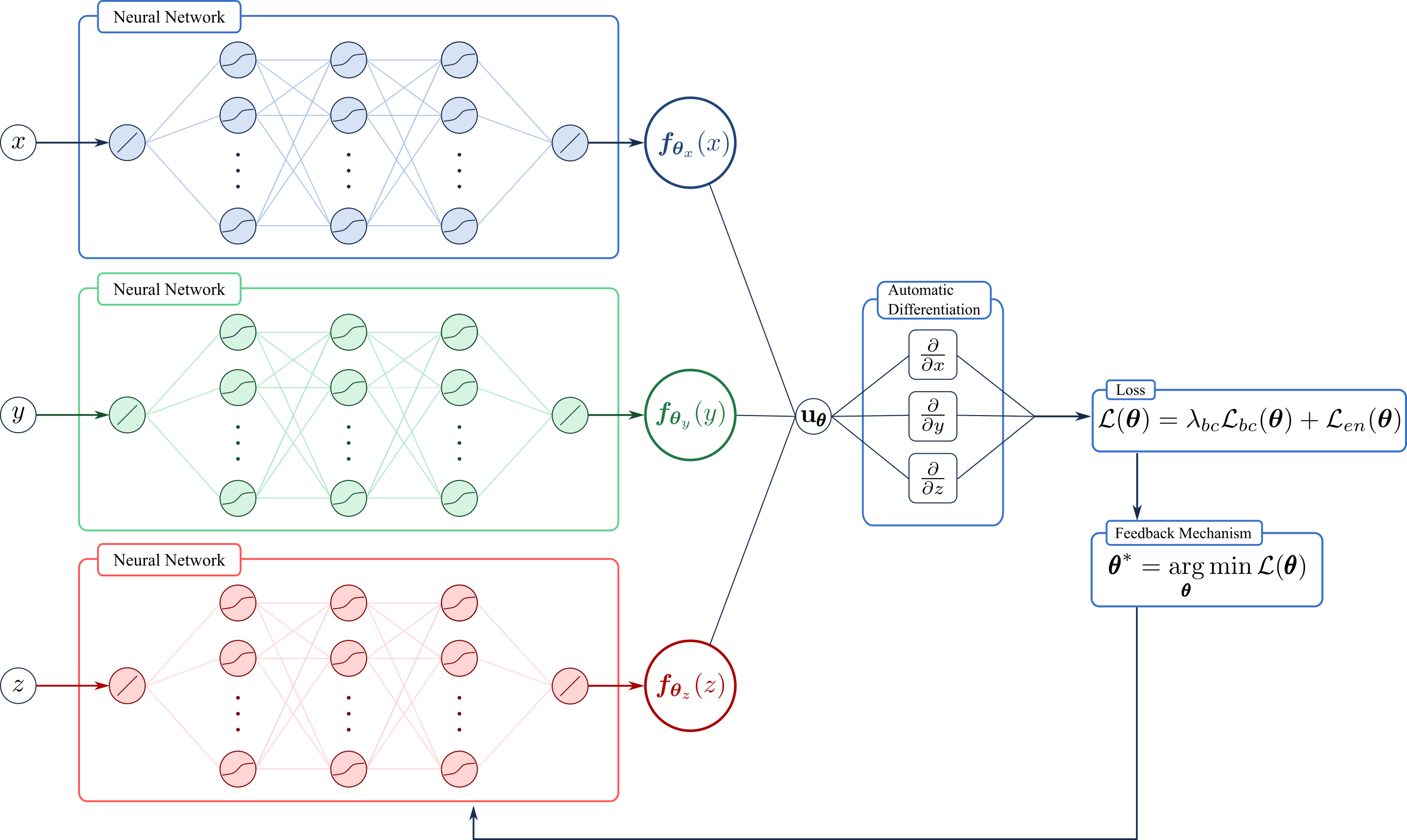
Figure 2: Schematic diagram of the deep energy method for the SPINN approach.

A schematic diagram of the general PINN method is shown in Figure 1.

4 Numerical experiments

To evaluate the accuracy of the approximate solution obtained with the help of the PINN method, the values of the solution of the linear elasticity problem predicted by the neural networks at given points are compared with the values calculated on the basis of the classical high-precision numerical method (FEM). The relative total ${\mathbb{L}}_{2}$ error of prediction is taken as a measure of accuracy, which can be expressed with the following relation

$$\epsilon_{\rm error}=\left\{\frac{1}{N_{e}}\sum^{N_{e}}_{i=1}\left[{\bf u}^{\boldsymbol{\theta}}({\bf x}_{i})-{\bf u}({\bf x}_{i})\right]^{2}\right\}^{1/2}\times\left\{\frac{1}{N_{e}}\sum^{N_{e}}_{i=1}\left[{\bf u}({\bf x}_{i})\right]^{2}\right\}^{-1/2},$$ (25)

where $\left\{{\bf x}_{i}\right\}^{N_{e}}_{i=1}$ is the set of evaluation points taken from the domain $\Omega$ of body, ${\bf u}_{\boldsymbol{\theta}}$ and ${\bf u}$ are the predicted and reference solutions respectively.

Relative total ${\mathbb{L}}_{2}$ errors were analyzed for the displacement components separately, for the magnitude of the displacements, which are given by

$$u_{\rm m}=\left(u_{x}^{2}+u_{y}^{2}+u_{z}^{2}\right)^{1/2},$$ (26)

and von Mises stress

$$\sigma_{\rm vM}=\left[\frac{3}{2}\sigma_{ij}\sigma_{ij}-\frac{1}{2}\left(\sigma_{kk}\right)^{2}\right]^{1/2}.$$ (27)

For our experiments we used Pytorch [58] version 1.12.1 as backend for Modulus, and Jax, which was used with code based on the source code is available at https://github.com/stnamjef/SPINN of paper [50]. The training was carried out on a node with Nvidia Tesla V100 GPU.

Reference values were obtained using OpenFOAM at CPU. There are presented the timespan of calculations of reference values in tables 2 and 5 considering the mesh generation time.

Description	Values for the beam problem	Values for the thin-walled angle problem
$E$ (Young modulus) (Pa)	$2.1\times 10^{11}$
$\nu$ (Poisson ratio)	0.3
$T$ (traction on external boundary) (Pa)	$10^{4}$	$2.5\times 10^{4}$
$g$ (gravitational acceleration) (m/s2)	9.81
$\rho$ (density of body material) (kg/m3)	$7.8\times 10^{3}$

Table 1: Parameters for the problems (material is steel)

For improving the training convergence and accuracy [59, 17] we transformed the original Eqs.(1)–(6) to the non–dimensionalized forms. The non–dimensionalized variables are defined as follows

$$\tilde{x}_{i}=\frac{x_{i}}{L_{c}},\quad\tilde{u}_{i}=\frac{u_{i}}{U_{c}},\quad\tilde{\lambda}=\frac{\lambda}{\mu_{c}},\quad\tilde{\nu}=\frac{\mu}{\mu_{c}},$$ (28)

where $L_{c}$ is the characteristic length, $U_{c}$ is the characteristic displacement, and $\mu_{c}$ is the non–dimensionalizing shear modulus. The non–dimensionalized state of a static equilibrium problem can be written as follows:

$$\frac{\partial\tilde{\sigma}_{ik}}{\partial\tilde{x}_{k}}+\tilde{f}_{i}=0,\,\quad\tilde{{\bf x}}\in\tilde{\Omega}$$ (29)

$$\tilde{\sigma}_{ik}n_{k}=\tilde{T}_{i},\quad\tilde{\bf x}\in\partial\tilde{\Omega},$$ (30)

$$\tilde{\bf u}=\tilde{\bf u}^{(b)},\quad\tilde{\bf x}\in\partial\tilde{\Omega},$$ (31)

where the non–dimensionalized forces and stress tensor are

$$\tilde{\sigma}_{ik}=\frac{L_{c}}{\mu_{c}U_{c}}{\sigma}_{ik},\quad\tilde{f}_{i}=\frac{L_{c}^{2}}{\mu_{c}U_{c}}{f}_{i},\quad\tilde{T}_{i}=\frac{L_{c}}{\mu_{c}U_{c}}T_{i}.$$ (32)

The values $\tilde{\bf u}^{(b)}$, $\tilde{\Omega}$ and $\partial\tilde{\Omega}$ are ${\bf u}^{(b)}$, $\Omega$ and $\partial\Omega$ were taken in transformed coordinates. Non–dimensionalized stress–displacement and strain–displacement relations are obtained by multiplying of equations (4) and (5) by $L_{c}/(\mu_{c}U_{c})$ and $L_{c}/U_{c}$, respectively, and have the following forms

$$\tilde{\sigma}_{ik}=\tilde{\lambda}\tilde{\varepsilon}_{ll}\delta_{ik}+\tilde{\mu}\tilde{\varepsilon}_{ik},$$ (33)

$$\tilde{\varepsilon}_{ik}=\frac{1}{2}\left(\frac{\partial\tilde{u}_{i}}{\partial\tilde{x}_{k}}+\frac{\partial\tilde{u}_{k}}{\partial\tilde{x}_{i}}\right).$$ (34)

4.1 Beam

Consider a beam made of an isotropic homogeneous elastic material with length $L=1$ m, width $W=0.1$ m and height $H=0.1$ m (see Fig. 3). So the coordinates of points of the beam ($x,y,z$) is satisfied to relations $x\in[0,1]$, $y\in[0,0.1]$, $z\in[0,0.1]$). The beam is fixed on boundary $x=0$, and is loaded by pressure ${\bf T}=-T{\bf z}_{0}$ on boundary $z=0.1$ m and gravity force ${\bf f}=-\rho g{\bf z}_{0}$ in each point of the body. Parameters of materials and magnitudes of forces are given in Table 1.

The undimensionalization parameters were chosen as $L_{c}=L$, $\mu_{c}=0.01\mu$ and $U_{c}=10^{-4}$ m.

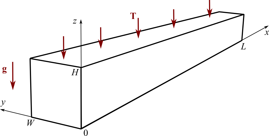
Figure 3: Beam with uniform load $\bf T$ in the gravity force $\bf g$

$$\frac{\partial\tilde{\sigma}_{xx}}{\partial\tilde{x}}+\frac{\partial\tilde{\sigma}_{xy}}{\partial\tilde{y}}+\frac{\partial\tilde{\sigma}_{xz}}{\partial\tilde{z}}=0,$$

$$\frac{\partial\tilde{\sigma}_{xy}}{\partial\tilde{x}}+\frac{\partial\tilde{\sigma}_{yy}}{\partial\tilde{y}}+\frac{\partial\tilde{\sigma}_{yz}}{\partial\tilde{z}}=0,$$

$$\frac{\partial\tilde{\sigma}_{xz}}{\partial\tilde{x}}+\frac{\partial\tilde{\sigma}_{yz}}{\partial\tilde{y}}+\frac{\partial\tilde{\sigma}_{zz}}{\partial\tilde{z}}-\tilde{\rho}g=0,$$

$$\tilde{u}_{x}=0,\quad\tilde{u}_{y}=0,\quad\tilde{u}_{z}=0\quad\text{in}\quad\tilde{x}=0,$$

$$\tilde{\sigma}_{zz}=-\tilde{T},\quad\tilde{\sigma}_{xz}=0,\quad\tilde{\sigma}_{yz}=0\quad\text{in}\quad\tilde{z}=0.1,$$

$$\tilde{\sigma}_{ik}=0,\quad\text{in}\quad\tilde{z}=0,\quad\tilde{x}=1\quad\tilde{y}=0,\quad\tilde{y}=0.1.$$ (35)

Here $\tilde{\rho}={L_{c}^{2}\rho}/{(\mu_{c}U_{c})}$ and $\tilde{T}={L_{c}T}/{(\mu_{c}U_{c})}$.

4.1.1 PINN

The PINN approach was implemented on the basis of Modulus from Nvidia with recommended parameters for the linear elasticity problems [59]. Each value of displacements and stress components are predicted with the help of the individual feedforward neural network (9 MLPs in the sum). Each MLP has 6 hidden layers with 512 neurons per layer. The activation function of these MLPs is “swish” function $[\text{swish}(x)=x\ \text{sigmoid}(x)]$.

The networks had been trained via stochastic gradient descent using the Adam optimizer [60]. The initial value of the learning rate is $10^{-3}$. Training consisted of 2,000,000 epochs for the method based on PDE. Weight factors $\lambda_{bc}$ in the loss function in Eq. (12) is set to 10. The training is based on 50,000 collocation points for the inner area of the beam (volumetric points) and 1664 points for the surface (surface points).

4.1.2 SPINN in the case of the loss based on PDE

The values of displacements and stresses are approximated with two different neural networks. First of which predicts three components of vector $\tilde{\bf u}$, second neural network predicts six components of tensor $\tilde{\sigma}_{ik}$. Due to this circumstance the loss function (12) must be added by term

$$\mathcal{L}_{u\sigma}({\bm{\theta}})=\frac{1}{N_{r}}\sum_{j=1}^{N_{r}}\sum_{i=1}^{3}\sum_{k=1}^{3}\left|\tilde{\sigma}_{ik}^{{\bm{\theta}}}-\left\{\tilde{\lambda}\frac{\partial\tilde{u}^{{\bm{\theta}}}_{l}}{\partial\tilde{x}_{l}}\delta_{ik}+\frac{\tilde{\mu}}{2}\left(\frac{\partial\tilde{u}^{{\bm{\theta}}}_{i}}{\partial\tilde{x}_{k}}+\frac{\partial\tilde{u}^{{\bm{\theta}}}_{k}}{\partial\tilde{x}_{i}}\right)\right\}\right|^{2},$$ (36)

and $\sigma_{ik}$ should be changed by $\tilde{\sigma}_{ik}^{{\bm{\theta}}}$ in all expressions (13)–(16). We will name this approach SPINN–PDE in our paper for brevity.

4.1.3 SPINN conjunction with DEM

In the SPINN approach, each neural network (for displacements or stresses predictions) consists of the three body–networks. Each body–network is a single MLP which has 3 hidden layers with 64 neurons per layer and 64 output values that play roles of the basis functions. The activation function of these MLPs is “swish” function. We will name this approach SPINN–DEM in our paper for brevity.

The networks had been trained via stochastic gradient descent using the Adam optimizer [60] and scheduler, which reduces the learning rate by 5% every 5,000 epochs (decay–rate is 0.95). The initial value of the learning rate is $10^{-3}$. Training consisted of 500,000 epochs for the method based on PDE and 100,000 epochs for the DEM. Weight factors $\lambda_{bc}$ in the loss function in Eq. (12) is set to 100. The training is based on $N_{r}=32^{3}$ collocation points ($32$ points for every axis) which are resampled every 100 epochs, except the SPINN–DEM approach, where the points were fixed. Evaluating the results of training carried out every 1000 epochs. Every training for this approach is performed 7 times with different seeds.

4.1.4 Comparison of the results

The experiments were carried out for all the above-mentioned methods: PINN based on PDE, SPINN based on PDE, and SPINN based on the DEM. In table 2 we present the timespan of one experiment, speed of training, and GPU memory consumption for these approaches. It can be seen that SPINN bypasses the PINN by a large margin both in speed and in memory using efficiency. In table 3 we also report the accuracy for the beam problem achieved using different methods for $u_{x,y,z}$, $u_{\rm m}$ and $\sigma_{\rm vM}$. As can be seen from this table the best result is achieved with SPINN based on DEM for all values while PINN and SPINN demonstrate close results.

In the table 4 are given times to achieve “engineering” accuracy ${\mathbb{T}}_{5\%}$ for the different values obtained by different approaches (in seconds). We defined “engineering” accuracy as relative error which should be less or equal 5$\%$ (${\mathbb{L}}_{2}\leq 0.05$). This table demonstrates the significant superiority of the SPINN based on DEM over the other methods in the speed of achieving the target accuracy of values.

The displacements and value of von Mises stress predicted by SPINN based on DEM, reference values obtained by FEM, and absolute errors are presented in Fig. 4. As you can see, SPINN gives distributions of values very close to the reverences. The most pronounced difference is observed in the von Mises stress at the place of fixing of the beam. However, distributions found by SPINN is more smooth in the points of fixation than distributions given by FEM. In our opinion, this smoothness of solutions that are obtained by SPINN indicates that this solution is closer to the real physical distributions than the one given by the FEM.

Method	Runtime (s)	Speed (epochs/s)	GPU Memory (MB)
FEM (based on PDE (7)–(9), at CPU)	4	—	—
PINN (Modulus, loss (12))	277515	7	14501
SPINN–PDE	$1869.86\pm 3.47$	283	733
SPINN–DEM	$356.54\pm 3.70$	295	723

Table 2: Beam problem: Timespan of one experiment, speed of training and GPU memory consumption for different approach

Method	${\mathbb{L}}_{2}[u_{x}]$	${\mathbb{L}}_{2}[u_{y}]$	${\mathbb{L}}_{2}[u_{z}]$	${\mathbb{L}}_{2}[u_{\rm m}]$	${\mathbb{L}}_{2}[\sigma_{\rm vM}]$
PINN (Modulus, loss (12))	0.0327	0.4465	0.0348	0.0348	—
SPINN–PDE	$\underset{\pm 0.0034}{0.0155}$	$\underset{\pm 0.0123}{0.3252}$	$\underset{\pm 0.0034}{0.0129}$	$\underset{\pm 0.0034}{0.0129}$	$\underset{\pm 0.0005}{0.0719}$
SPINN–DEM	$\underset{\pm 0.0010}{0.0025}$	$\underset{\pm 0.0089}{0.0281}$	$\underset{\pm 0.0008}{0.0030}$	$\underset{\pm 0.0008}{0.0030}$	$\underset{\pm 0.0049}{0.0419}$

Table 3: Beam problem: Relative ${\mathbb{L}}_{2}$ errors obtained by different approaches for the different values

Method	${\mathbb{T}}_{5\%}[u_{x}]$	${\mathbb{T}}_{5\%}[u_{y}]$	${\mathbb{T}}_{5\%}[u_{z}]$	${\mathbb{T}}_{5\%}[u_{\rm m}]$	${\mathbb{T}}_{5\%}[\sigma_{\rm vM}]$
SPINN–PDE	$\underset{\pm 57.44}{441.48}$	—	$\underset{\pm 48.77}{426.84}$	$\underset{\pm 48.77}{426.84}$	—
SPINN–DEM	$\underset{\pm 2.67}{9.75}$	$\underset{\pm 19.84}{55.08}$	$\underset{\pm 2.67}{9.75}$	$\underset{\pm 2.67}{9.75}$	$\underset{\pm 20.97}{112.54}$

Table 4: Beam problem: Times to achieve “engineering” accuracy ${\mathbb{T}}_{5\%}$ for the different values obtained by different approaches (in seconds). “Engineering” accuracy is defined by relative error which should be less or equal 5$\%$ (${\mathbb{L}}_{2}\leq 0.05$).

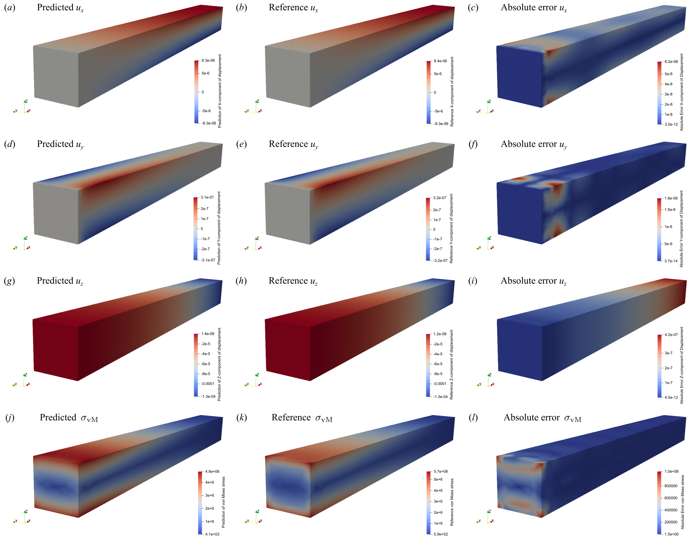
Figure 4: Beam problem: (a), (d), (g) and (j) are the predictions of a trained physics-informed neural network; (b), (e), (h) and (k) are reference solutions; (c), (f), (i) and (l) are absolute values of differences between reference and predicted solutions, for the value $u_{x}$, $u_{y}$, $u_{z}$ and $\sigma_{\rm vM}$, respectively.

4.2 Thin-walled angle

Consider a thin-walled angle made of an isotropic homogeneous elastic material with length $L=1$ m, width $W=0.06$ m, height $H=0.06$ m, and the wall thickness $d=6\times 10^{-3}$ m (see Fig. 5). So the coordinates of points of the angle ($x,y,z$) is satisfied to relations

$$x\in[0,1],\quad(y,z)\in[0,0.06]\times[0,0.06],\quad(y,z)\notin[0,0.054]\times[0,0.054].$$

The angle is fixed on boundary $x=0$, and is loaded by pressure ${\bf T}=-T{\bf z}_{0}$ on boundary $z=0.06$ m and gravity force ${\bf f}=-\rho g{\bf z}_{0}$ in each point of the body. Parameters of materials and magnitudes of forces are given in Table 1.

The non-dimensional parameters were chosen as $L_{c}=L$, $\mu_{c}=\mu$ and $U_{c}=10^{-4}$ m.

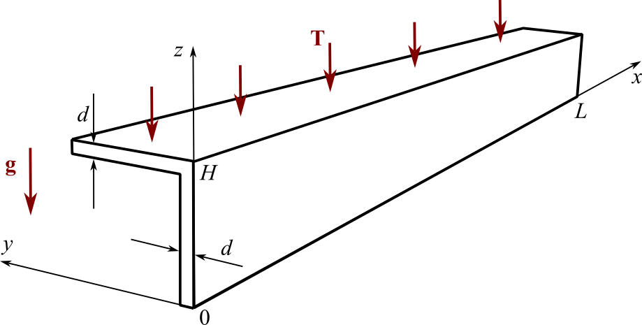
Figure 5: Thin-walled angle with uniform load $\bf T$ in the gravity force $\bf g$

Note, that no one method (vanilla PINN and SPINN) based on the partial differential equations (12) did not converge to reference solutions in our experiments.

In the SPINN–DEM approach every element of the displacements vector is predicted by an individual neural network. Each such neural network consists of the three body–networks. Each body–network is a single MLP which has 5 hidden layers with 64 neurons per layer and 64 output values which play roles of the basis functions. The activation function of these MLPs is “swish” function.

The networks had been trained via stochastic gradient descent using the Adam optimizer [60] and scheduler, which reduces the learning rate by 5% every 5,000 epochs (decay–rate is 0.95). The initial value of the learning rate is $10^{-3}$. Training consisted of 200,000 epochs. Weight factors $\lambda_{bc}$ in the loss function in Eq. (18) is set to 1000. The domain of integration was separated on two domains: $[0,1]\times[0,0.06]\times[0,0.54]$ and $[0,1]\times[0,0.6]\times[0.054,0.06]$. The collocation points were taken on uniform grids. The number of points for the first and second domains is $513\times 9\times 65$ and $513\times 65\times 9$, respectively. Evaluating the results of training carried out every 1000 epochs. Every training for this approach is performed 7 times with different seeds.

In table 5 we present the duration of one experiment, speed of training, and GPU memory consumption for training of SPINN. It can be seen that SPINN has speed and memory efficiency close to the SPINN in the previous problem. In table 6 we also report the accuracy for the problem achieved using this method for $u_{x,y,z}$, $u_{\rm m}$ and $\sigma_{\rm vM}$. As can be seen from this table the results achieved with SPINN based on DEM are relatively good.

In the table 7 are given times to achieve “engineering” accuracy ${\mathbb{T}}_{5\%}$ for the different values obtained by this approach (in seconds). This table demonstrates the relatively good convergence time of SPINN to target accuracy.

The displacements and value of von Mises stress predicted by SPINN based on DEM, reference values obtained by FEM, and absolute errors are presented in Fig. 6. As before shown for the beam problem, SPINN gives distributions of values very close to the reverences once, and the most pronounced differences are laid in the von Mises stress at the place of fixing of the beam. The distributions found by SPINN look like more smooth in the fixed points than distributions given by FEM, and this smoothness of solutions indicates that this solution is closer to the real physical distributions than the one given by the FEM.

Method	Runtime (s)	Speed (epochs/s)	GPU Memory (MB)
FEM (based on PDE (7)–(9), at CPU)	35	—	—
SPINN–DEM	$2159.64\pm 24.1$	95	989

Table 5: Thin-walled angle problem: Duration of one experiment, speed of training and GPU memory consumption for different approach

Method	${\mathbb{L}}_{2}[u_{x}]$	${\mathbb{L}}_{2}[u_{y}]$	${\mathbb{L}}_{2}[u_{z}]$	${\mathbb{L}}_{2}[u_{\rm m}]$	${\mathbb{L}}_{2}[\sigma_{\rm vM}]$
SPINN–DEM	$\underset{\pm 0.0003}{0.0038}$	$\underset{\pm 0.0037}{0.0389}$	$\underset{\pm 0.0017}{0.0205}$	$\underset{\pm 0.0014}{0.0173}$	$\underset{\pm 0.0034}{0.0807}$

Table 6: Thin-walled angle problem: Relative ${\mathbb{L}}_{2}$ errors obtained by SPINN–DEM approach

Method	${\mathbb{T}}_{5\%}[u_{x}]$	${\mathbb{T}}_{5\%}[u_{y}]$	${\mathbb{T}}_{5\%}[u_{z}]$	${\mathbb{T}}_{5\%}[u_{\rm m}]$	${\mathbb{T}}_{5\%}[\sigma_{\rm vM}]$
SPINN–DEM	$\underset{\pm 29.70}{127.69}$	$\underset{\pm 209.73}{1291.20}$	$\underset{\pm 112.89}{760.34}$	$\underset{\pm 56.46}{646.89}$	—

Table 7: Thin-walled angle problem: Times to achieve “engineering” accuracy ${\mathbb{T}}_{5\%}$ for the different values obtained by SPINN–DEM approach (in seconds). “Engineering” accuracy is defined by relative error which should be less or equal to 5$\%$ (${\mathbb{L}}_{2}\leq 0.05$).

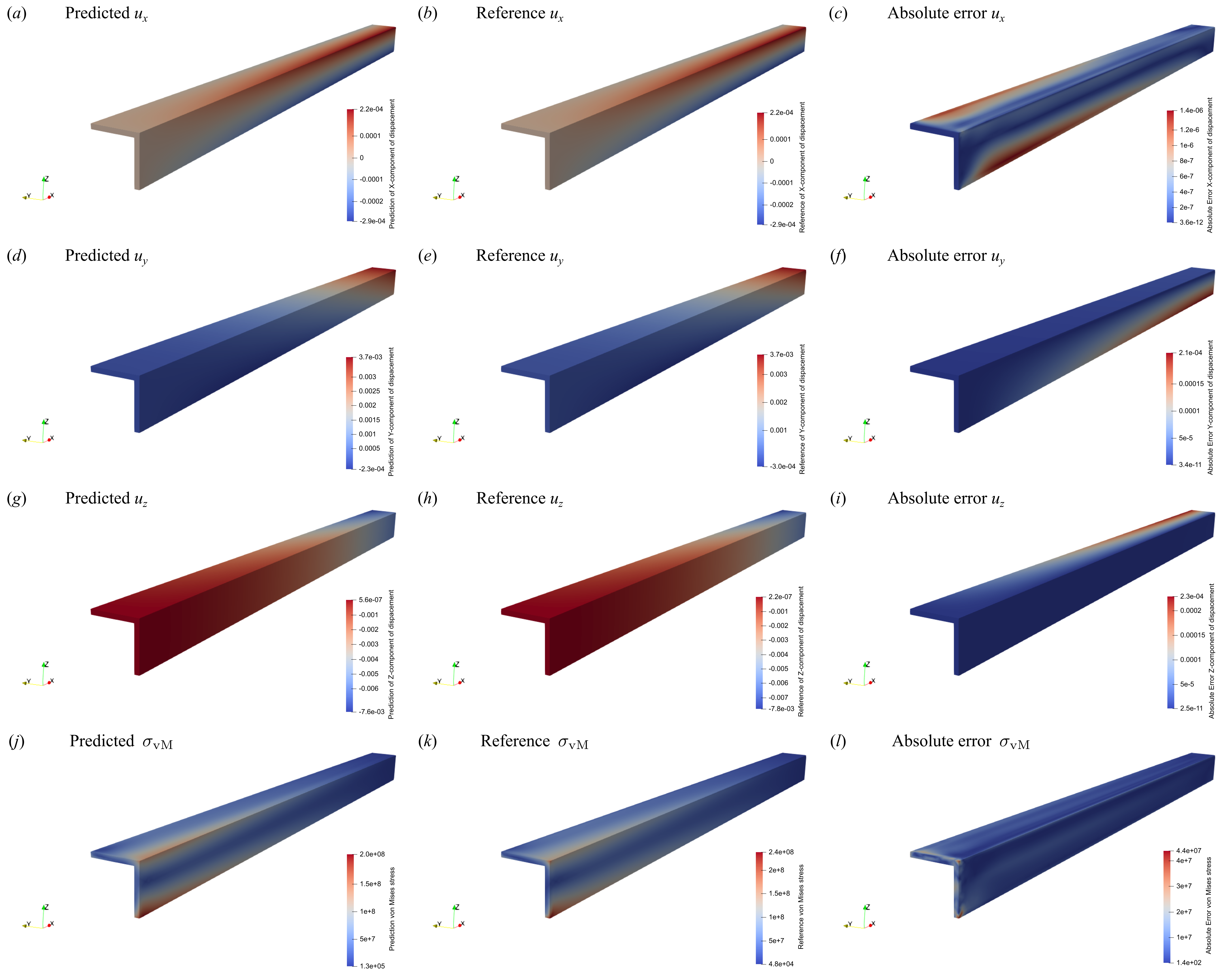
Figure 6: Thin-walled angle problem: (a), (d), (g) and (j) are prediction of a trained physics-informed neural network; (b), (e), (h) and (k) are reference solutions; (c), (f), (i) and (l) are absolute values of differences between reference and predicted solutions, for the value $u_{x}$, $u_{y}$, $u_{z}$ and $\sigma_{\rm vM}$, respectively..

5 Conclusion

In this article, we presented the method for solving elasticity problems based on separable physics-informed neural networks in conjunction with the deep energy method. The performance of this approach had been compared with the performances of the other method which are based on the solution of the partial differential equations which describe the elasticity problems. This comparison shows that the SPINN–DEM method has a convergence rate and accuracy that significantly exceeds the speed of convergence and accuracy of vanilla PINN and SPINN–PDE. In terms of the speed of solving of the problems, this method approaches the classical numerical finite element methods (FEM). In addition, the authors’ claim about original SPINN [50] is confirmed, that SPINN-based solution methods consume much less GPU memory than the vanilla PINN. Note another important feature of the methods of the PINN family is a significantly smaller amount of memory occupied by a trained neural network compared to the stored data which generated by classical FEMs. It was demonstrated that separable physics-informed neural networks in the framework of the deep energy method solve problems of the linear elasticity on complex geometries, which is not available to solve when using the PINNs in frames of partial differential equations. The proposed method without significant changes can be used for a number of other elasticity problems [43, 48].

Appendix A Nomenclature

The summarizes the main notations, abbreviations and symbols are given in table 8.

Notation	Description
MLP	Multilayer perceptron
PDE	Partial differential equation
PINN	Physic-informed neural network
DEM	Deep energy method
SPINN	Separable Physics-Informed Neural Networks
SPINN–PDE	SPINN for the loss problem based on PDE
SPINN–DEM	SPINN in conjunction with the deep energy method (loss is energy loss)
${\bf u}$	solution of problem
${\mathcal{B}}$	boundary operator
$\mathcal{R}$	PDE residual
${\bf u}^{\boldsymbol{\theta}}$	neural network representation of the problem solution
${\boldsymbol{\theta}}$	vector of the trainable parameters of the neural network
${\mathcal{L}(\boldsymbol{\theta})}$	aggregate training loss

Table 8: Nomenclature

References

- [1] Laith Alzubaidi, Jinglan Zhang, Amjad J Humaidi, Ayad Al Dujaili, Ye Duan, Omran Al Shamma, J Santamaría, Mohammed A Fadhel, Muthana Al Amidie, and Laith Farhan. Review of deep learning: concepts, CNN architectures, challenges, applications, future directions. Springer International Publishing, 2021.
- [2] Yann LeCun, Yoshua Bengio, and Geoffrey Hinton. Deep learning. Nature, 521(7553):436–444, may 2015.
- [3] Pantelis Linardatos, Vasilis Papastefanopoulos, and Sotiris Kotsiantis. Explainable AI: A Review of Machine Learning Interpretability Methods. Entropy, 23(1), 2021.
- [4] Salman Khan, Muzammal Naseer, Munawar Hayat, Syed Waqas Zamir, Fahad Shahbaz Khan, and Mubarak Shah. Transformers in Vision: A Survey. ACM Comput. Surv., 54(10s), sep 2022.
- [5] Ashish Vaswani, Samy Bengio, Eugene Brevdo, Francois Chollet, Aidan N. Gomez, Stephan Gouws, LLion Jones, Lukasz Kaiser, Nal Kalchbrenner, Niki Parmar, Ryan Sepassi, Noam Shazeer, and Jakob Uszkoreit. Tensor2Tensor for Neural Machine Translation, 2018.
- [6] Qiang Wang, Bei Li, Tong Xiao, Jingbo Zhu, Changliang Li, Derek F. Wong, and Lidia S. Chao. Learning Deep Transformer Models for Machine Translation, 2019.
- [7] Shaowei Yao and Xiaojun Wan. Multimodal transformer for multimodal machine translation. In Proceedings of the 58th Annual Meeting of the Association for Computational Linguistics, pages 4346–4350, Online, July 2020. Association for Computational Linguistics.
- [8] Aditya Ramesh, Mikhail Pavlov, Gabriel Goh, Scott Gray, Chelsea Voss, Alec Radford, Mark Chen, and Ilya Sutskever. Zero-Shot Text-to-Image Generation, 2021.
- [9] Stanislav Frolov, Tobias Hinz, Federico Raue, Jörn Hees, and Andreas Dengel. Adversarial text-to-image synthesis: A review. Neural Networks, 144:187–209, 2021.
- [10] David Silver, Thomas Hubert, Julian Schrittwieser, Ioannis Antonoglou, Matthew Lai, Arthur Guez, Marc Lanctot, Laurent Sifre, Dharshan Kumaran, Thore Graepel, Timothy Lillicrap, Karen Simonyan, and Demis Hassabis. A general reinforcement learning algorithm that masters chess, shogi, and Go through self-play. Science, 362(6419):1140–1144, 2018.
- [11] Julian Schrittwieser, Ioannis Antonoglou, Thomas Hubert, Karen Simonyan, Laurent Sifre, Simon Schmitt, Arthur Guez, Edward Lockhart, Demis Hassabis, Thore Graepel, Timothy Lillicrap, and David Silver. Mastering Atari, Go, chess and shogi by planning with a learned model. Nature, 588(7839):604–609, dec 2020.
- [12] Long Ouyang, Jeff Wu, Xu Jiang, Diogo Almeida, Carroll L. Wainwright, Pamela Mishkin, Chong Zhang, Sandhini Agarwal, Katarina Slama, Alex Ray, John Schulman, Jacob Hilton, Fraser Kelton, Luke Miller, Maddie Simens, Amanda Askell, Peter Welinder, Paul Christiano, Jan Leike, and Ryan Lowe. Training language models to follow instructions with human feedback, 2022.
- [13] M Raissi, P Perdikaris, and G E Karniadakis. Physics-informed neural networks: A deep learning framework for solving forward and inverse problems involving nonlinear partial differential equations. Journal of Computational Physics, 378:686–707, 2019.
- [14] Sifan Wang, Shyam Sankaran, and Paris Perdikaris. Respecting causality is all you need for training physics-informed neural networks. 2022. arXiv:2203.07404.
- [15] Haifeng Wang, Xu Qian, Yabing Sun, and Songhe Song. A Modified Physics Informed Neural Networks for Solving the Partial Differential Equation with Conservation Laws. —.
- [16] Vasiliy A. Es’kin, Danil V. Davydov, Ekaterina D. Egorova, Alexey O. Malkhanov, Mikhail A. Akhukov, and Mikhail E. Smorkalov. About optimal loss function for training physics-informed neural networks under respecting causality, 2023. arXiv:2304.02282.
- [17] Sifan Wang, Shyam Sankaran, Hanwen Wang, and Paris Perdikaris. An expert’s guide to training physics-informed neural networks, 2023. arXiv:2308.08468.
- [18] Lu Lu, Pengzhan Jin, Guofei Pang, Zhongqiang Zhang, and George Em Karniadakis. Learning nonlinear operators via DeepONet based on the universal approximation theorem of operators. Nature Machine Intelligence, 3(3):218–229, mar 2021.
- [19] Zongyi Li, Daniel Zhengyu Huang, Burigede Liu, and Anima Anandkumar. Fourier Neural Operator with Learned Deformations for PDEs on General Geometries. 2022. arXiv:2207.05209.
- [20] Mikhail A. Krinitskiy, Victor M. Stepanenko, Alexey O. Malkhanov, and Mikhail E. Smorkalov. A General Neural-Networks-Based Method for Identification of Partial Differential Equations, Implemented on a Novel AI Accelerator. Supercomputing Frontiers and Innovations, 9(3), sep 2022.
- [21] V. Fanaskov and I. Oseledets. Spectral Neural Operators. 2022. arXiv:2205.10573.
- [22] Oded Ovadia, Adar Kahana, Panos Stinis, Eli Turkel, and George Em Karniadakis. ViTO: Vision Transformer-Operator. mar 2023. arXiv:2303.08891.
- [23] Hanxun Jin, Enrui Zhang, Boyu Zhang, Sridhar Krishnaswamy, George Em Karniadakis, and Horacio D. Espinosa. Mechanical characterization and inverse design of stochastic architected metamaterials using neural operators, 2023. arXiv:2311.13812.
- [24] Maziar Raissi, Paris Perdikaris, and George Em Karniadakis. Physics Informed Deep Learning (Part I): Data-driven Solutions of Nonlinear Partial Differential Equations. (Part I):1–22. arXiv:1711.10561v1.
- [25] Maziar Raissi, Paris Perdikaris, and George Em Karniadakis. Physics Informed Deep Learning (Part II): Data-driven Discovery of Nonlinear Partial Differential Equations. (Part II):1–19. arXiv:1711.10566v1.
- [26] Shengze Cai, Zhicheng Wang, Frederik Fuest, Young Jin Jeon, Callum Gray, and George Em Karniadakis. Flow over an espresso cup: inferring 3-d velocity and pressure fields from tomographic background oriented schlieren via physics-informed neural networks. Journal of Fluid Mechanics, 915, March 2021.
- [27] Dimitris C. Psichogios and Lyle H. Ungar. A hybrid neural network-first principles approach to process modeling. Aiche Journal, 38:1499–1511, 1992.
- [28] I.E. Lagaris, A. Likas, and D.I. Fotiadis. Artificial neural networks for solving ordinary and partial differential equations. IEEE Transactions on Neural Networks, 9(5):987–1000, 1998.
- [29] Christopher Rackauckas, Yingbo Ma, Julius Martensen, Collin Warner, Kirill Zubov, Rohit Supekar, Dominic Skinner, Ali Ramadhan, and Alan Edelman. Universal Differential Equations for Scientific Machine Learning. pages 1–55, jan 2020. arXiv:2001.04385.
- [30] Lei Yuan, Yi-Qing Ni, Xiang-Yun Deng, and Shuo Hao. A-PINN: Auxiliary physics informed neural networks for forward and inverse problems of nonlinear integro-differential equations. Journal of Computational Physics, 462:111260, aug 2022.
- [31] Xiaowei Jin, Shengze Cai, Hui Li, and George Em Karniadakis. NSFnets (Navier-Stokes flow nets): Physics-informed neural networks for the incompressible Navier-Stokes equations. Journal of Computational Physics, 426:109951, 2021.
- [32] Lifei Zhao, Zhen Li, Zhicheng Wang, Bruce Caswell, Jie Ouyang, and George Em Karniadakis. Active- and transfer-learning applied to microscale-macroscale coupling to simulate viscoelastic flows. Journal of Computational Physics, 427:110069, 2021. arXiv:2005.04382.
- [33] Ehsan Kharazmi, Zhongqiang Zhang, and George E.M. Karniadakis. hp-VPINNs: Variational physics-informed neural networks with domain decomposition. Computer Methods in Applied Mechanics and Engineering, 374:113547, 2021. arXiv:2003.05385.
- [34] Liu Yang, Xuhui Meng, and George Em Karniadakis. B-PINNs: Bayesian physics-informed neural networks for forward and inverse PDE problems with noisy data. Journal of Computational Physics, 425:109913, 2021. arXiv:2003.06097.
- [35] Salvatore Cuomo, Vincenzo Schiano di Cola, Fabio Giampaolo, Gianluigi Rozza, Maziar Raissi, and Francesco Piccialli. Scientific Machine Learning through Physics-Informed Neural Networks: Where we are and What’s next. jan 2022. arXiv:2201.05624.
- [36] G. Pang, M. D’Elia, M. Parks, and G. E. Karniadakis. nPINNs: Nonlocal physics-informed neural networks for a parametrized nonlocal universal Laplacian operator. Algorithms and applications. Journal of Computational Physics, 422:109760, 2020. arXiv:2004.04276.
- [37] Ravi G. Patel, Indu Manickam, Nathaniel A. Trask, Mitchell A. Wood, Myoungkyu Lee, Ignacio Tomas, and Eric C. Cyr. Thermodynamically consistent physics-informed neural networks for hyperbolic systems. Journal of Computational Physics, 449:110754, jan 2022. arXiv:2012.05343.
- [38] Bokai Liu, Yizheng Wang, Timon Rabczuk, Thomas Olofsson, and Weizhuo Lu. Multi-scale modeling in thermal conductivity of polyurethane incorporated with phase change materials using physics-informed neural networks. Renewable Energy, 220:119565, 2024.
- [39] Shengze Cai, Zhiping Mao, Zhicheng Wang, Minglang Yin, and George Em Karniadakis. Physics-informed neural networks (PINNs) for fluid mechanics: a review. Acta Mechanica Sinica, 37(12):1727–1738, dec 2021.
- [40] Guochang Lin, Pipi Hu, Fukai Chen, Xiang Chen, Junqing Chen, Jun Wang, and Zuoqiang Shi. BINet: Learning to Solve Partial Differential Equations with Boundary Integral Networks. pages 1–27, oct 2021. arXiv:2110.00352.
- [41] QiZhi He, David Barajas-Solano, Guzel Tartakovsky, and Alexandre M. Tartakovsky. Physics-informed neural networks for multiphysics data assimilation with application to subsurface transport. Advances in Water Resources, 141:103610, jul 2020.
- [42] Ehsan Haghighat, Maziar Raissi, Adrian Moure, Hector Gomez, and Ruben Juanes. A physics-informed deep learning framework for inversion and surrogate modeling in solid mechanics. Computer Methods in Applied Mechanics and Engineering, 379:113741, 2021.
- [43] Zeng Meng, Qiaochu Qian, Mengqiang Xu, Bo Yu, Ali Rıza Yıldız, and Seyedali Mirjalili. Pinn-form: A new physics-informed neural network for reliability analysis with partial differential equation. Computer Methods in Applied Mechanics and Engineering, 414:116172, 2023.
- [44] E. Samaniego, C. Anitescu, S. Goswami, V.M. Nguyen-Thanh, H. Guo, K. Hamdia, X. Zhuang, and T. Rabczuk. An energy approach to the solution of partial differential equations in computational mechanics via machine learning: Concepts, implementation and applications. Computer Methods in Applied Mechanics and Engineering, 362:112790, 2020.
- [45] Luyuan Ning, Zhenwei Cai, Han Dong, Yingzheng Liu, and Weizhe Wang. A peridynamic-informed neural network for continuum elastic displacement characterization. Computer Methods in Applied Mechanics and Engineering, 407:115909, 2023.
- [46] W.Q. Hao, L. Tan, X.G. Yang, D.Q. Shi, M.L. Wang, G.L. Miao, and Y.S. Fan. A physics-informed machine learning approach for notch fatigue evaluation of alloys used in aerospace. International Journal of Fatigue, 170:107536, 2023.
- [47] Ben Moseley, Andrew Markham, and Tarje Nissen-Meyer. Solving the wave equation with physics-informed deep learning. jun 2020. arXiv:2006.11894.
- [48] Luyuan Ning, Zhenwei Cai, Han Dong, Yingzheng Liu, and Weizhe Wang. Physics-informed neural network frameworks for crack simulation based on minimized peridynamic potential energy. Computer Methods in Applied Mechanics and Engineering, 417:116430, 2023.
- [49] Ali Harandi, Ahmad Moeineddin, Michael Kaliske, Stefanie Reese, and Shahed Rezaei. Mixed formulation of physics-informed neural networks for thermo-mechanically coupled systems and heterogeneous domains. International Journal for Numerical Methods in Engineering, November 2023.
- [50] Junwoo Cho, Seungtae Nam, Hyunmo Yang, Seok-Bae Yun, Youngjoon Hong, and Eunbyung Park. Separable physics-informed neural networks, 2023. arXiv:2306.15969.
- [51] Lev D Landau and Evgeny M Lifshitz. Theory of Elasticity. Volume 7 if Course of Theoretical Physics. Pergamon press, third edition, 1986.
- [52] Kurt Hornik, Maxwell Stinchcombe, and Halbert White. Multilayer feedforward networks are universal approximators. Neural Networks, 2(5):359–366, 1989.
- [53] Andreas Griewank and Andrea Walther. Evaluating Derivatives. Society for Industrial and Applied Mathematics, second edition, 2008.
- [54] Sifan Wang, Yujun Teng, and Paris Perdikaris. Understanding and Mitigating Gradient Flow Pathologies in Physics-Informed Neural Networks. SIAM Journal on Scientific Computing, 43(5):A3055—-A3081, 2021.
- [55] Sifan Wang, Xinling Yu, and Paris Perdikaris. When and why PINNs fail to train: A neural tangent kernel perspective. Journal of Computational Physics, 449:110768, 2022.
- [56] Anthony L. Caterini and Dong Eui Chang. Generic Representation of Neural Networks, pages 23–34. Springer International Publishing, Cham, 2018.
- [57] Siddhartha Mishra and Roberto Molinaro. Estimates on the generalization error of physics-informed neural networks for approximating a class of inverse problems for PDEs. IMA Journal of Numerical Analysis, 42(2):981–1022, 06 2021.
- [58] Adam Paszke, Sam Gross, Francisco Massa, Adam Lerer, James Bradbury, Gregory Chanan, Trevor Killeen, Zeming Lin, Natalia Gimelshein, Luca Antiga, Alban Desmaison, Andreas Köpf, Edward Yang, Zach DeVito, Martin Raison, Alykhan Tejani, Sasank Chilamkurthy, Benoit Steiner, Lu Fang, Junjie Bai, and Soumith Chintala. PyTorch: An Imperative Style, High-Performance Deep Learning Library. Curran Associates Inc., Red Hook, NY, USA, 2019.
- [59] NVIDIA Modulus v22.09 linear elasticity. https://docs.nvidia.com/deeplearning/modulus/modulus-v2209/user_guide/foundational/linear_elasticity.html#:~:text=Modulus%20offers%20the%20capability%20of,a%20variety%20of%20boundary%20conditions. Accessed: 2023-11-21.
- [60] Diederik P. Kingma and Jimmy Ba. Adam: A Method for Stochastic Optimization, 2014.