Ordering kinetics in the active Ising model

Abstract

We undertake a numerical study of the ordering kinetics in the two-dimensional ($2d$) active Ising model (AIM), a discrete flocking model with a non-conserved scalar order parameter. We find that for a quench into the liquid-gas coexistence region and in the ordered liquid region, the characteristic length scale of both the density and magnetization domains follows the Lifshitz-Cahn-Allen (LCA) growth law: $R(t)\sim t^{1/2}$, consistent with the growth law of passive systems with scalar order parameter and non-conserved dynamics. The system morphology is analyzed with the two-point correlation function and its Fourier transform, the structure factor, which conforms to the well-known Porod’s law, a manifestation of the coarsening of compact domains with smooth boundaries. We also find the domain growth exponent unaffected by different noise strengths and self-propulsion velocities of the active particles. However, transverse diffusion is found to play the most significant role in the growth kinetics of the AIM. We extract the same growth exponent by solving the hydrodynamic equations of the AIM.

I Introduction

Active matter systems involve the movement of large assemblies of individual active particles that consume energy to self-propel and exhibit collective behavior in a non-equilibrium steady state Ramaswamy (2010); Marchetti et al. (2013); Needleman and Dogic (2017); Gompper et al. (2020). Collective motion is ubiquitous in nature, observed in a wide array of different living systems over a range of scales, from macroscopic fields like fleets of birds Ballerini et al. (2008) and schools of fish Becco et al. (2006); Calovi et al. (2014) to microscopic scales like hoards of bacteria Steager et al. (2008); Peruani et al. (2012), cytoskeletal filaments and molecular motors Schaller et al. (2010); Sumino et al. (2012); Sanchez et al. (2012). It leads to the emergence of ordered motion of large clusters, called flocks, with a typical size larger than an individual Ramaswamy (2010); Vicsek and Zafeiris (2012); Shaebani et al. (2020); De Magistris and Marenduzzo (2015); Krishnan et al. (2010). Over the past two decades, new models have emerged to understand the various physical principles governing active matter systems Shaebani et al. (2020).

Vicsek and collaborators years ago introduced a minimal model Vicsek et al. (1995) of active particles that move with a constant speed and orient via a ferromagnetic interaction with a neighborhood similar to the XY model. In the Vicsek model (VM) activity can stabilize the ordered phase even in two dimensions which is not possible in the $2d$ XY model where the long-range fluctuation destroys the ordered phase following Mermin-Wagner theorem  Toner and Tu (1995, 1998). Then, about a decade ago, Solon and Tailleur introduced the active Ising model (AIM) Solon and Tailleur (2013, 2015) where the continuous rotational symmetry of the VM is replaced by a discrete symmetry. In the AIM, each particle assumes two possible states allowing the particle to propel in a preferred direction which changes upon interaction with other particles at the same lattice site. The AIM retains the essential part of the VM physics and exhibits flocking behavior with three different phases at steady state: disordered gas at high noise and low densities, polar liquid at low noise and high densities, and a phase-separated liquid-gas coexistence state at intermediate densities. However, a key difference between the VM and the AIM arises in the steady-state behavior of the coexistence region. In this region, AIM shows a macrophase separation associated with normal density fluctuations whereas the VM is characterized by a microphase separation with giant density fluctuations. The flocking transition in the AIM is a first-order liquid-gas phase transition similar to the VM, however, for zero activity, despite the dynamics being non-equilibrium, the AIM shows a second-order phase transition belonging to the Ising universality class.

Although significant progress has been made to understand the steady state properties of various active systems Toner et al. (2005); Giomi et al. (2013); Cates and Tailleur (2015); Solon et al. (2015); Siebert et al. (2018); Wysocki and Rieger (2020); Mangeat et al. (2020); Chatterjee et al. (2020a); Kürsten and Ihle (2020); Fruchart et al. (2021); Solon et al. (2022); Chatterjee et al. (2022); Codina et al. (2022); Chatterjee et al. (2023); Karmakar et al. (2023), there is much to explore in the realm of ordering kinetics in active systems that relaxes to a non-equilibrium steady state (NESS). Understanding the intrinsic non-equilibrium dynamics that drive an active system towards its steady state is of fundamental as well as practical relevance. Unlike active systems, ordering kinetics in non-equilibrium passive systems have been studied over several decades Bray (2002, 1994); Puri (2009); Ahmad et al. (2012); Shrivastav et al. (2014); Kumar et al. (2017); Chatterjee et al. (2020b). Domain growth in passive systems with non-conserved scalar order parameters follows the Lifshitz-Cahn-Allen (LCA) growth law: $R(t)\sim t^{1/2}$ (Model A of order-parameter kinetics) whereas passive systems with conserved order parameter follow a Lifshitz-Slyozov-Wagner (LSW) growth law: $R(t)\sim t^{1/3}$ (Model B of order-parameter kinetics), $R$ being average size of domains. Using tools that quantify the kinetics of passive systems, several active systems have been explored. These include Active Model B Wittkowski et al. (2014); Pattanayak et al. (2021a, b), active nematics Mishra et al. (2014), self-propelled particles in disordered medium Das et al. (2018), Model B with nonreciprocal activity Saha et al. (2020), Kuramoto oscillators Rouzaire and Levis (2022), active Brownian particles Dittrich et al. (2023) and motility-induced phase separated (MIPS) clusters Caporusso et al. (2023). Moreover, an interesting observation of multiple coarsening length scales was made in the prototypical VM Katyal et al. (2020) where velocities are found to align over a faster-growing length scale compared to density. Another intriguing result of an active system with a non-conserved vector order parameter following the growth law of the non-conserved scalar order parameter field has also been observed Dikshit and Mishra (2023). Since AIM is a minimal flocking model with a rich phase behavior, studying the growth kinetics of this model will allow us to interpret the origin of large flocks in terms of microscopic interactions.

In this paper, we explore the phase ordering kinetics of the AIM with a non-conserved scalar order parameter. Quenching the AIM inside the spinodal region results in the formation of small positively or negatively magnetized clusters which in the late stage of the coarsening merge to form a single, macroscopic domain of one spin type Solon and Tailleur (2015). A few questions arise in this context: (a) Does the domain morphology follow the same pattern and growth law for quenches into the coexistence and in the ordered liquid region? (b) Since the order parameter is non-conserved in AIM, how does the growth law relate to the established growth law of similar passive systems? (c) Do the density and magnetization align over the same length scale? Katyal et al. (2020) (d) What is the impact of noise and particle activity on the domain growth? and (e) What is the role of diffusion in the domain growth dynamics? We address these issues by analyzing the ordering dynamics of the $2d$ AIM on a square lattice via Monte Carlo simulations and by solving the AIM hydrodynamic equations using the finite difference method.

This paper is organized as follows. In Sec. II we discuss the model and then present the details of numerical simulations in Sec. III. In Sec.IV, we present the growth law of the AIM from both numerical simulation and hydrodynamic description. Finally, in Sec. V, we conclude this paper with a summary and discussion of the results.

II Model

We consider $N$ particles on a two-dimensional square lattice $L\times L$ with periodic boundary conditions. Thus the average particle density is $\rho_{0}=N/L^{2}$. Each lattice site $i$ can accommodate an arbitrary number of particles $n_{i}^{\sigma}$ with spin $\sigma=\pm 1$. Defining local density $\rho_{i}=n_{i}^{+}+n_{i}^{-}$ and magnetization $m_{i}=n_{i}^{+}-n_{i}^{-}$ we note that $\rho_{i}$ has no upper bound, while $m_{i}$ is bounded by $\rho_{i}$: $-\rho_{i}\leq m_{i}\leq\rho_{i}$. Each particle with a given spin state $\sigma$ can either flip to $-\sigma$ or jump to a nearest-neighbor site probabilistically.

The flipping rates are derived from a local ferromagnetic Potts Hamiltonian Mangeat et al. (2020); Chatterjee et al. (2020a) defined as:

$$H_{i}=-\frac{J}{2\rho_{i}}\sum_{k=1}^{\rho_{i}}\sum_{l\neq k}\left(q\delta_{\sigma_{i}^{k},\sigma_{i}^{l}}-1\right)\,,$$ (1)

where $J$ is the coupling between any two particles at site $i$ and the Kronecker delta $\delta_{\sigma_{i}^{k},\sigma_{i}^{l}}$ survives only for $\sigma_{i}^{k}=\sigma_{i}^{l}$. Eq. (1) with $q=2$ is the local Hamiltonian defined for the AIM Solon and Tailleur (2015). Local interaction implies that a particle can align with the average direction of all other particles at the same site.

The spin-flip transition rates are derived from the Potts Hamiltonian $H_{\rm APM}=\sum_{i}H_{i}$ according to the energy difference before and after the spin flip. For $q=2$, a particle with spin $\sigma$ flips its state according to the transition rate  (Mangeat et al., 2020; Chatterjee et al., 2020a):

$$W_{\rm flip}(\sigma\rightarrow-\sigma)=\gamma\exp\left[-\frac{2\beta J}{\rho_{i}}\left(\sigma m_{i}-1\right)\right]\,,$$ (2)

where $\gamma$ is the rate of particle flipping when $\sigma m_{i}=1$. In this paper, we choose $J=1$, and $\gamma=1$ without any loss of generality. The parameter $\beta$, denoted as “inverse temperature”, $\beta=T^{-1}$, in passive systems, controls the flip noise strength. Although the system under consideration is athermal, we denote the parameter $T$ as “temperature” from now on.

Moreover, each particle performs a biased diffusion on the lattice depending on the spin state $\sigma$. For $q=2$ particles perform a one-dimensional biased hopping along the $\pm x$-direction with the following hopping rate Mangeat et al. (2020); Chatterjee et al. (2020a):

$$W_{\rm hop}(\sigma,p)=D\left[1+\epsilon({2\delta_{\sigma,p}-1})\right]\,,$$ (3)

where $p$ denotes the direction of bias-hopping ($p=+1$ along the $+x$ direction and $p=-1$ along the $-x$ direction). The presence of other particles does not influence hopping rates and hence is independent of particle density. The hopping rate $D=1$ is constant along the upward and downward directions ($\pm y$-direction). The parameter $\epsilon\in[0,1]$ $(0\leq\epsilon\leq q-1)$ controls the asymmetry between the purely diffusive limit $\epsilon=0$ and the purely ballistic limit $\epsilon=1$, while $D$ controls the overall hopping rate. On average, a particle drifts with speed $v=2D\epsilon$ in the direction set by the sign of its spin state (where lattice spacing is 1), while the total hopping rate $4D$, remains constant.

III Simulation details

A Monte Carlo (MC) simulation of the stochastic process defined above evolves in unit Monte Carlo steps (MCS) $\Delta t$ resulting from a microscopic time $\Delta t/N$. During $\Delta t/N$, a randomly chosen particle with spin $\sigma$ flips with probability $W_{\rm flip}\Delta t$ or hops to one of the neighboring sites with probability $W_{\rm hop}\Delta t$. Consequently, $1-[4D+W_{\rm flip}]\Delta t$ is the probability that the particle does nothing, and minimizing this we obtain $\Delta t=[4D+\exp(2\beta)]^{-1}$.

To study the morphology of the system during phase ordering kinetics, we use the two-point equal-time $(t)$ correlation function of the local scalar order parameters. The notion utilizes the spatial fluctuations in the density and magnetization fields to estimate Dikshit and Mishra (2023):

$$C_{\rho\rho}(r,t)=\frac{1}{L^{2}}\sum_{i=1}^{L^{2}}\langle\Delta\rho_{i,t}\Delta\rho_{i+r,t}\rangle$$ (4)

$$C_{mm}(r,t)=\frac{1}{L^{2}}\sum_{i=1}^{L^{2}}\langle\Delta m_{i,t}\Delta m_{i+r,t}\rangle\,,$$ (5)

where $\langle\cdots\rangle$ denotes averaging over independent initial realizations, $\Delta\rho_{i,t}=\rho_{i}-\rho_{0}$ and $\Delta m_{i,t}=m_{i}-m_{0}$ are the local fluctuations in density and magnetization from the mean, respectively. The above definition of $C_{\rho\rho}$ characterizes the morphology of the spatial structures and $C_{mm}$ evaluates the correlations in the polar alignment among the evolving structures separated by a distance $r$. Since we observe that $C_{\rho\rho}$ and $C_{mm}$ behave similarly in the AIM (see below), we focus here on $C_{\rho\rho}$, which we denote as $C$ [$C_{\rho\rho}(r,t)\equiv C(r,t)$] from now on. Following a temperature quench from a random initial configuration into the ordered state, domains of both spin types appear and grow with time. Similar morphology of the evolving domains with average domain size $R(t)$ would correspond to a dynamical scaling relation Puri (2009); Bray (2002, 1994):

$$C(r,t)=f\left(\frac{r}{R(t)}\right)$$ (6)

where $f(x)$ is a time-independent scaling function. $R(t)$, estimated from the decay of $C(r,t)$ generally show a power-law growth Puri (2009); Bray (2002, 1994):

$$R(t)\sim t^{\theta}\,,$$ (7)

with $\theta$ as the growth exponent. Typically, the morphology of an ordering system is studied by scattering experiments, which measure the structure factor $S(k,t)$, defined by the Fourier transform of the correlation function $C(r,t)$:

$$S(k,t)=\int_{-\infty}^{\infty}C(r,t)e^{ikr}dr\,,$$ (8)

and has a dynamical scaling form in $d$ dimensions:

$$S(k,t)=R(t)^{d}g\left[kR(t)\right]\,.$$ (9)

For scalar order parameters like the density field, the short-distance (large-$k$) behavior of the structure factor scaling function is given by the Porod’s law (for domains with smooth boundaries or scattering off sharp domain interfaces) which corresponds to $g(k)\sim k^{-(d+1)}$. Next, we present results for model parameters set by the average particle density $\rho_{0}$, temperature $T=\beta^{-1}$, self-propulsion velocity $\epsilon$, and diffusion constant $D$.

IV Results

IV.1 Phase diagram and domain morphology

The steady-state behavior of the AIM is summarized in the temperature-density ($T-\rho_{0}$) [Fig. 1(a)] and velocity-density ($\epsilon-\rho_{0}$) [Fig. 1(b)] phase diagrams. The general structure of the phase diagrams consists of a gas phase (G), a liquid phase (L), and a liquid-gas coexistence region (G+L) separated by the gas and liquid binodals. Qualitatively similar results were obtained earlier in Ref. Solon and Tailleur (2015). However, we obtain a critical temperature $T_{c}\simeq 2$ (above which no phase separation occurs irrespective of the density, critical density $\rho_{c}=\infty$) twice as large as in Ref. Solon and Tailleur (2015). This can be understood if one compares the flipping rate of Ref. Solon and Tailleur (2015), $W_{\rm flip}(\sigma\rightarrow-\sigma)=\gamma\exp\left(-\sigma\beta\frac{m_{i}}{\rho_{i}}\right)$ with Eq. (2) for $J=1$ which denotes that the effective $\beta$ considered in this paper is roughly twice as large as the $\beta$ of Ref. Solon and Tailleur (2015). In the $\epsilon-\rho_{0}$ phase diagram, the two binodals converge at a critical density $(\rho_{c}\simeq 2.9)$ for vanishing self-propulsion ($\epsilon=0$) which signifies a second-order phase transition belonging to the Ising universality class Solon and Tailleur (2013).

We chose to quench the random initial systems in two different regimes of the temperature-density phase diagram shown by the arrows in Fig. 1(a). The quench occurs instantaneously from a very high-temperature regime ($T\rightarrow\infty$) shown by the blue stars to the liquid-gas coexistence region or the polar liquid region, denoted by red stars, with the same final temperature $T=0.9$ ($T<T_{c}$, corresponds to $\beta=1.1$) but different densities.

To quantify the coarsening dynamics we performed simulations on a square lattice of size $400^{2}$ with periodic boundary conditions applied on both sides. Following quench at time $t=0$, the system is evolved up to $t=10^{5}$ using the MC algorithm described in Sec. III. All numerical data presented here are averaged over at least 300 independent realizations.

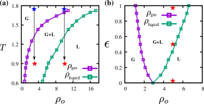
Figure 1: (Color online) Phase diagrams of the AIM showing the quench directions at fixed densities. (a) $(T,\rho_{0})$ phase diagram for self-propulsion velocity $\epsilon=1$. (b) $(\epsilon,\rho_{0})$ phase diagram at fixed temperature $T=0.9$. G and L denote the disordered gas and polar liquid regions whereas G+L denotes the phase-coexistence region. The blue stars indicate the initial high-temperature points in the phase diagram from where the system is quenched (indicated by arrows) into the coexistence region ($\rho_{0}=3$) and to the liquid region ($\rho_{0}=10$) [red stars]. $\rho_{\rm gas}$ and $\rho_{\rm liquid}$ are the gas and liquid binodal, respectively.

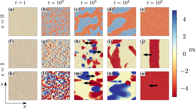
Figure 2: (Color online) Time evolution snapshots of the local magnetization field on a $400^{2}$ system after a quench from $T=\infty$ to $T=0.9$ for $\epsilon=0$ (top panel) and $\epsilon=1$ (middle and lower panel). The color bar denotes magnetization per site. (a–e) Curvature-driven domain growth of the diffusive Ising model ($\rho_{0}=5$, $\epsilon=0$). (f–j) Growth dominated by the dynamics of spinodal decomposition after the system is quenched inside the spinodal region ($\rho_{0}=3$, $\epsilon=1$) and (k–o) domain growth mediated by the merging of high-density clusters of $\sigma=\pm 1$ after the system is quenched deep inside the ordered liquid regime ($\rho_{0}=10$, $\epsilon=1$). Black arrows denote the direction of the movement of the clusters and bands.

A typical simulation of coarsening dynamics starts with a homogeneous initial configuration where particles with $\sigma=\pm 1$ are distributed randomly on each lattice site. This can also be described as an equilibrium configuration at infinite temperature because all configurations are equally likely. Then, after a quench well below the critical temperature ($T_{c}\simeq 2$), the homogeneous initial configuration starts evolving in time, and subsequent dynamics are governed by the formation and growth of $\sigma=1$ and $\sigma=-1$ rich domains. Such a time evolution of the local magnetization field is shown in Fig. 2 for $\epsilon=0$ and $\epsilon=1$. In the latter scenario, time evolution has been shown for a quench in both the coexistence (middle row) and liquid regions (bottom row). The non-equilibrium steady states (NESS) are characterized by a single band (at lower density) and a polar liquid (at higher density).

The top panel, Fig. 2(a–e), depicts the ordering kinetics of a purely diffusive $(\epsilon=0)$ polar liquid at $\rho_{0}=5$. The domain morphology with increasing time exhibits a close resemblance with the passive Ising model Majumder and Das (2011). In the Ising model, the driving force for the domain growth is the curvature of the domain wall since the system surface energy can only decrease through a reduction in the total net surface area. In the $\epsilon=0$ limit, particles do not form high-density domains due to the diffusive movement of particles. Therefore, density-wise, the system remains homogeneous as we observe a steady growth of small, high-curvature to large, low-curvature domains. This is unsurprising as the $2d$ AIM for $\epsilon=0$ belongs to the same universality class of the passive $2d$ Ising model Solon and Tailleur (2015).

Next, we looked at the evolution of AIM with self-propulsion velocity ($\epsilon=1$) quenching the system inside the spinodal [Fig. 2(f–j)] and homogeneous ordered regions [Fig. 2(k–o)]. The average densities representing these two regions correspond to $\rho_{0}=3$ and 10, respectively. Inside the spinodal region, the growth dynamics are driven by spinodal decomposition and result in the formation of numerous small clusters of negative and positive spins $(t=10^{2})$. The coarsening then stems from the merging of these clusters $(t=10^{3}$ and $t=10^{4})$, until a single, macroscopic domain emerges $(t=10^{5})$ in the steady state. A quench deep inside the homogeneous ordered region also results in similar dynamics of cluster formation and coalescence of those clusters into a single large liquid domain (in this paper, for $\epsilon>0$, the word cluster is used interchangeably with domain). With extreme self-propelled particles ($\epsilon=1$), although the high-density clusters are strongly biased along the horizontal directions, they can also grow along the transverse direction due to the constant transverse diffusion $D$. When these clusters merge into a larger cluster, it always tries to minimize the surface energy by decreasing the surface area. Accordingly, the coarsening process leads to a single band [Fig. 2(j)] with domain walls having the lowest curvature (the curvature of a straight line is zero but a liquid band with a perfectly straight domain boundary can only happen when there is no thermal fluctuation). The focus of this study is, therefore, to analyze the coarsening dynamics shown in Fig. 2 which we will do next.

IV.2 Dynamical scaling

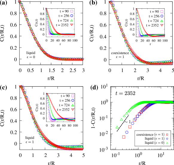
Figure 3: (Color online) (a–c) Scaled correlation functions $C(r/R,t)$ versus $r/R$, for the evolution of the $2d$ AIM shown in Fig. 2. Unscaled versions are shown in the inset. “Liquid” and “coexistence” signify the region where the system is quenched, $\epsilon$ denotes particle speed. (d) Log-log plot of $1-C(r/R)$ versus $r/R$. The cusp exponent is estimated as $\alpha\sim 1$. Parameters correspond to Fig. 2.

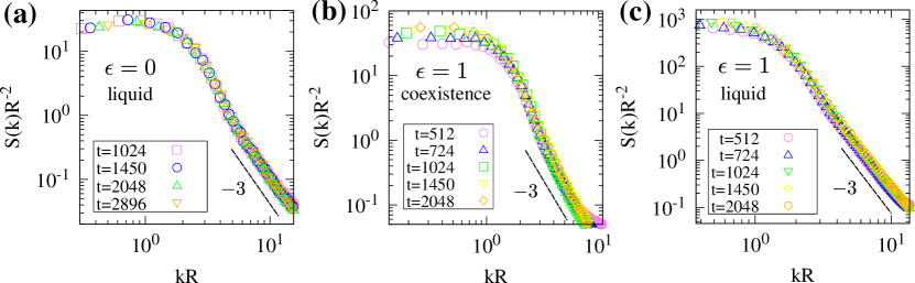
Figure 4: (Color online) (a–c) Scaled structure factors, $S(k,t)R(t)^{-2}$ versus $kR$, for the Fourier transform of the correlation function data sets corresponding to the same values of time. The line of slope $\simeq-3$ denotes the Porod’s law: $S(k)\sim k^{-(d+1)}$ for $d=2$.

In the theory of phase-ordering kinetics, the scaling hypothesis states that if the system is characterized by a single length scale $R(t)$ [$R(t)$ is equivalent to the average domain size], the domain morphology is statistically the same at all times, apart from a scale factor. When all domain lengths are measured in units of $R(t)$, the equal-time pair correlation function should exhibit the dynamical-scaling property of Eq. (6). The equal-time correlation function is a non-equilibrium quantity so as $R(t)$ which can be estimated from the decay of the correlation function. To identify the self-similar behavior of the evolving domains we plot the correlation function in Fig. 3. The scaled $C(r/R,t)$ and unscaled $C(r,t)$ correlation functions are shown in Fig. 3(a–c) for $\epsilon=0$ and $\epsilon=1$. $R(t)$ is determined from the distance over which the correlation function decays to e.g., 0.2 of its maximum value, that is, $C(r,t)=0.2C(0,t)$.

As the system coarsens, the correlation function decays slowly [insets of Fig. 3(a–c)], signifying the growth of the characteristic length scale $R(t)$. Upon rescaling the spatial coordinates by this length scale, the correlation function at different times collapses onto a single function $C(r/R,t)$ as shown in Fig. 3(a–c), thus confirming a universal coarsening behavior with time. Such scaling behavior implies that the structure is time-invariant and consistent with a power-law growth of $R(t)$ with increasing $t$. This scaling hypothesis is satisfied when the growing length is much smaller than the system size to avoid the finite size effect. We further examine the AIM domain morphology by approximating the small distance behavior of the scaled two-point correlation function

$$1-C(r)=\bar{C}(r)\sim r^{\alpha}$$ (10)

in Fig. 3(d) which yields the cusp exponent $\alpha\sim 1$. This signifies the existence of sharp domain interfaces [see Fig. 2(h) and Fig. 2(m)] and translates into the power-law behavior of the scaled structure factor plotted in Fig. 4 Shrivastav et al. (2014). Fig. 3(d) also signifies that the domain structure of the AIM for $\epsilon=1$ is statistically self-similar for quenches into the coexistence and liquid region whereas different from the domain morphology of the AIM for $\epsilon=0$, as evident from Fig. 2.

In Fig. 4, we plot the scaled structure factor, $S(k,t)R(t)^{-2}$ versus $kR$, which is the Fourier transform of the correlation function. In Fourier space, Eq. (10) translates into the following power-law behavior of the structure factor: $S(k)\sim k^{-(d+\alpha)}$ and therefore, the large-$k$ behavior of the structure factor tail generates a slope $\sim-3$ (in log-log plot) for $d=2$ and $\alpha=1$ which denotes “Porod’s decay”: $S(k)\sim k^{-(d+1)}$, associated with scattering from sharp interfaces Bray (2002, 1994). This naturally originates from the long-range ordering in AIM leading to compact high-density clusters with smooth boundaries. Domains with rough morphologies having fractal interfaces do not follow Porod’s law and the large-$k$ tail of the scaled structure factor yields a non-integer exponent Chatterjee et al. (2018). A similar violation of the Porod law was also observed in the coarsening of the VM due to the irregular morphology associated with the cluster boundaries Dey et al. (2012); Katyal et al. (2020). $C(r,t)$ [and consequently, $S(k,t)$] exhibits two distinct power laws for small and large $r/R$ limits [large and small $kR$ limits] in the VM Dey et al. (2012) which we do not observe in the AIM. Furthermore, density fluctuations might also play a role in determining whether a system will follow or violate Porod’s law. In the VM, giant density fluctuations break large liquid domains and restrict the formation of large compact domains (which eventually manifests in the microphase separation of the coexistence region in the steady-state) Solon et al. (2015) and might be responsible for the non-Porod behavior of the system Dey et al. (2012). On the other hand, AIM obeys the Porod behavior where density fluctuations are normal in the liquid phase Solon and Tailleur (2015) and the steady-state manifests a bulk phase separation.

IV.3 Growth law

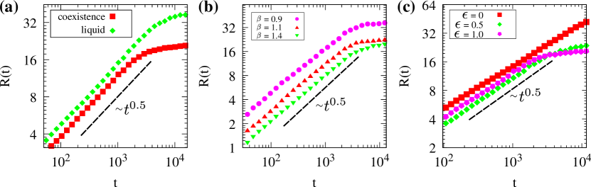
Figure 5: (Color online) (a) $R(t)\sim t^{1/2}$ for a quench into the coexistence and liquid regimes. The late time saturation of $R(t)$ signifies that the system has reached the corresponding NESS. As the density is higher for the liquid quench, the saturation appears late. Parameters: $\rho_{0}=3$ (coexistence), $\rho=10$ (liquid), $L=400$, $\beta=1.1$ and $\epsilon=1$. (b) $R(t)$ versus $t$ for different thermal noises ($T=\beta^{-1}$, coexistence regime). Parameters: $L=400$, $\rho_{0}=3$ and $\epsilon=1$. (c) Role of self-propulsion on the characteristic length $R(t)$ as a function of $t$. For a larger $\epsilon$, the system reaches the NESS faster while for $\epsilon=0$, the corresponding dynamics is slow. Parameters: $L=400$, $\beta=1.1$, and $\rho_{0}=5$. The growth law $R(t)\sim t^{1/2}$ is unaffected by thermal fluctuations and particle activity.

In passive systems with non-conserved scalar order parameters, the late-stage domain growth is governed by the diffusive Lifshitz-Cahn-Allen (LCA) growth law $R(t)\sim t^{1/2}$ Bray (1994). For non-conserved systems described by scalar fields such as the Ising model, the growth process is driven by the diffusion of the domain walls (the simplest form of topological defect) caused by the local changes in the order parameter. Diffusion also influences coarsening in non-conserved systems with vector fields, such as the $2d$ XY model, where domain evolution occurs when point topological defects, such as vortices and anti-vortices, diffuse, interact, and annihilate Yurke et al. (1993). Both systems exhibit a diffusive growth exponent $\theta=\frac{1}{2}$ (in the XY model, $R(t)\sim(t/\ln t)^{1/2}$, the logarithmic correction is due to the free vortices Yurke et al. (1993)). Therefore, a 0.5 growth exponent signifies a coarsening process dominated by the diffusion of defects. For example, if the time evolution of a non-conserved scalar order parameter such as the magnetization $m$ follows the diffusive equation $\dot{m}=D\nabla^{2}m$, then the length scale will exhibit a $\sqrt{t}$ dependence.

Therefore, the immediate question one can ask is whether the LCA growth law also governs the late-stage coarsening dynamics of an active system with non-conserved scalar order parameters such as the AIM and whether the coarsening process is diffusion-dominated. To characterize this, we plot the length scale data with time in Fig. 5 for various control parameters and quench regimes. We find that the late-stage growth kinetics of the domain in the coexistence and liquid regimes exhibit a $R(t)\sim t^{1/2}$ growth law [Fig. 5(a)]. We extract the same growth law for different temperatures [Fig. 5(b)], and self-propulsion velocities [Fig. 5(c)]. Domains identified by the correlation of density and magnetization fields also show similar growth behavior (see Appendix A). An interesting feature of the domain growth kinetics is that the domain size for a quench into the liquid regime is larger than the corresponding domain size in the coexistence regime [see Fig. 2 at $t=10^{3}$ and Fig.5(a)], although the domain morphologies for both these quench regimes are self-similar. The larger domains in the liquid regime are likely to be arising from higher density. Also, notice that a larger $\beta$ in Fig. 5(b) signifies a reduced thermal noise that slows down the local ordering of spins. Thus smaller $\beta$ allows the formation of larger domains. Nevertheless, different thermal fluctuations exhibit the same growth as thermal noise is asymptotically irrelevant for ordering in systems that are free from disorder Puri (2009).

Fig. 5(c) shows the increasing length scale with time for different $\epsilon$. For $\epsilon=0$, the system is purely diffusive, and domain growth proceeds via the coarsening of connected domains (curvature-driven growth facilitated by diffusing domain wall) [see Fig. 2(c–d)]. The domain morphology looks very similar to the evolution of an Ising ferromagnet quenched below the critical temperature. Thus, a $\sim t^{1/2}$ growth law for $\epsilon=0$ similar to the pure Ising model is physically plausible. But, when $\epsilon>0$, the domains of each spin no longer remain connected and form high-density clusters that self-propel along the horizontal direction. As time progresses, these clusters spread in the transverse direction due to constant diffusion ($D=1$) and merge with other clusters. Therefore, the domain growth for $\epsilon>0$ is again a diffusive phenomenon, and consequently, the growth kinetics exhibits a $R(t)\sim t^{1/2}$ growth law similar to $\epsilon=0$. We have identified this novel mechanism of diffusion-driven domain growth in the AIM after a thorough investigation of the altered diffusion coefficient in Sec. IV.4 and Appendix B.

It should also be noted that while approaching the NESS via coarsening, the high-density AIM domains of individual spins, upon merging, try to minimize the surface energy by decreasing the surface area similar to the dynamics of the passive non-conserved scalar order parameter. Therefore, although the system is active, the critical mechanisms (diffusion-dominated growth and minimization of surface energy during coarsening) of domain coarsening in AIM are similar to the $2d$ Ising model, and thus, it is not surprising that we extract a $R(t)\sim t^{1/2}$ growth law for both the passive and active models. For a more precise quantification of the asymptotic growth law, we determine the effective growth exponent, defined as:

$$Z_{\rm eff}=\frac{d[\ln R(t)]}{d[\ln t]}\,.$$ (11)

In Fig. 6(a), we plot $Z_{\rm eff}$ versus $t$ for different $\epsilon$ corresponding to the data in Fig.5(c). All data show extended flat regimes at late times (after $\sim t>10^{2}$). The effective exponent turns out to be in the regime $0.45<Z_{\rm eff}<0.52$, denoted by the dashed lines. We perform a similar study for the quench into the coexistence and liquid regimes. Fig. 6(b) shows $Z_{\rm eff}$ vs. $t$ once again confirms $Z_{\rm eff}\sim 0.5$, irrespective of the quench regimes.

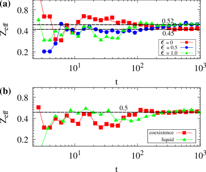
Figure 6: (Color online) Effective growth exponent $Z_{\rm eff}$ versus time $t$ for (a) different self-propulsion ($\epsilon=0,0.5$, and $1$, $\beta=1.1$ and $\rho_{0}=3$) and (b) quenching into different NESS ($\rho_{0}=3$ for coexistence and $\rho_{0}=10$ for liquid, $\beta=1.1$ and $\epsilon=1$). The dashed lines are a guide to the eyes.

IV.4 Role of transverse diffusion

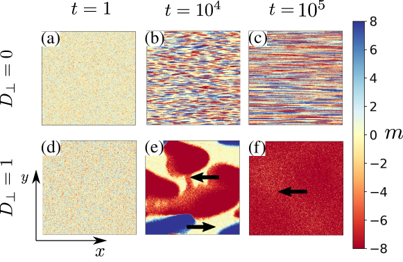
Figure 7: (Color online) Time evolution of the local magnetization field for $D_{\perp}=0$ [top panel, (a–c)] and $D_{\perp}=1$ [bottom panel, (d–f)] after quenching the system from a disordered gaseous phase to a high-density region. Parameters: $L=400,\beta=1.1$, $\rho_{0}=10$, and $\epsilon=1$.

In the AIM, particles self-propel only in the horizontal direction with average velocity $2D\epsilon$. The directional hopping of the particles is a function of the spin type ($+\sigma$ or $-\sigma$). To test the hypothesis that the late time domain growth in the AIM is also a diffusion-driven process, we decompose the diffusion into two components, $D_{\perp}$ (along $\pm y$ direction) and $D_{\parallel}$ (along $\pm x$ direction). We vary $D_{\perp}$, keeping $D_{\parallel}=D=1$ henceforth, and show the domain evolution in Fig.7.

The time evolution of the domains for $D_{\perp}=0$ is shown in Fig. 7(a–c). Starting from a disordered configuration, the time evolution of the system progresses via the formation of $1d$ rings with domains of alternating polarity along the horizontal direction ($x-$direction). These domains are one lattice unit wide along the transverse direction ($y-$direction) and are independent of the neighboring rings [Fig. 7(b)]. As particles can not diffuse along the transverse direction, these domains can only grow horizontally without merging with the neighboring rings. At late times, we observe narrow horizontal stripes of alternating magnetization [Fig. 7(c)]. Therefore, AIM with $D_{\perp}=0$ does not manifest the observed domain morphology representative of the growth law $\sim t^{1/2}$. $D_{\perp}=0$ also signifies $L_{y}$ numbers of one-dimensional periodic rings on which the AIM is defined. Such $1d$ AIM has been found to display flocking of a single dense ordered aggregate at intermediate temperatures (this flock undergoes stochastic reversals of its magnetization with time) but an aster phase consisting of sharp peaks of positive and negative magnetizations in a jammed state at lower temperatures Benvegnen et al. (2022). The one lattice unit-wide (along $y$) domains in Fig. 7(c) manifest the characteristics of the flocking state of $1d$ AIM for the given parameters (see Appendix B for details) but the system does not exhibit flocking as a whole since the $L_{y}$ number of $1d$ rings do not interact with each other for $D_{\perp}=0$. Altering the transverse diffusion $D_{\perp}$ to a nonzero value, particle diffusion occurs along the transverse $\pm y$ direction. Therefore, the random initial state coarsens to form high-density clusters which coarsen further to give rise to a large flocking domain [Fig. 7(d-f)].

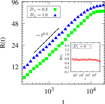
Figure 8: (Color online) $R(t)$ versus $t$ (on a log-log scale) showing a 0.5 growth exponent for different transverse diffusion $D_{\perp}=0.3$ and $D_{\perp}=1$. Inset: $R(t)$ versus $t$ in the absence of any transverse diffusion ($D_{\perp}=0$) showing no growth of domains with time. Parameters: $L=400$, $\beta=1.1$, $\epsilon=1$, and $\rho_{0}=8$.

To quantify the role of the magnitude of transverse diffusion coefficient ($D_{\perp}$), we plot $R(t)$ versus $t$ in Fig. 8 for two different values of $D_{\perp}$. The plot shows that the system exhibits the power-law growth of $R(t)\sim t^{1/2}$ for different values of $D_{\perp}$. Interestingly, even a small $D_{\perp}=0.3$ is sufficient to drive the proper domain growth. A larger $D_{\perp}$ only increases the average domain size. As discussed earlier in Fig. 7(b–c), a vanishing $D_{\perp}$ can not initiate a domain growth as $R(t)$ remains constant with $t$ (see inset of Fig. 8). Therefore, transverse diffusion plays the most crucial role in the AIM growth kinetics.

IV.5 Growth law from the hydrodynamic description of the AIM

In this section, we want to investigate whether the continuous description of the AIM also manifests the same time dependency $(\sim t^{1/2})$ of the coarsening length scale as observed in our numerical analysis. We consider refined mean-field equations similar to Ref. Solon and Tailleur (2015) for the spatiotemporal evolutions of the density $(\rho)$ and magnetization $(m)$ fields:

$$\dot{\rho}=D\nabla^{2}\rho-v\partial_{x}m\,,$$ (12)

$$\dot{m}=D\nabla^{2}m-v\partial_{x}\rho+2\left(2\beta-1-\frac{r}{\rho}\right)m-\alpha\frac{m^{3}}{\rho^{2}}\,,$$ (13)

where $v=2D\epsilon$, $\alpha=4\beta^{2}(1-2\beta/3)$, and $r=3\alpha\alpha_{m}/2$ is a positive function of $\beta$ Solon and Tailleur (2015). In constructing Eq. (13), we slightly modify the flipping rate equation of Eq. (2) to read $W_{\rm flip}=\exp\left(-2\beta\sigma m/\rho\right)$. For the mean-field equations, $r=0$, which can not capture the AIM physics correctly as the system always exhibits homogeneous profiles (gas and liquid), and the inhomogeneous phase-separated profiles are never observed Solon and Tailleur (2015). In Eqs. (12) and (13), local fluctuations are taken into account, which are generally neglected in the mean-field approximations Solon and Tailleur (2015).

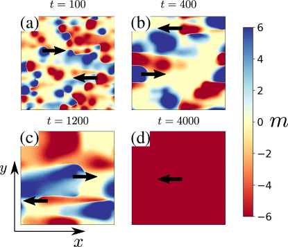
Figure 9: (Color online) Time evolution snapshots of the magnetization field $m$ obtained by solving the AIM hydrodynamic equations Eq. (12) and Eq. (13) after a quench from the homogeneous gaseous phase to an ordered liquid phase. Parameters: $L=400$, $\beta=0.75$, and $\rho_{0}=5$.

Eqs. (12) and (13) immediately show the importance of the transverse diffusion. If we start with a $x$-independent initial condition, for instance, a horizontal thin stripe of width $w$, where: $\rho(y)=\rho_{0}/w$, $m(y)=m_{0}>0$ is the stationary solution of Eq. (13) for $0<y<w$, and $\rho(y)=\delta\ll\rho_{0}/w$ and $m_{0}=0$ otherwise. Then the solution stays $x$-independent at all later times: $\rho(x,y,t)=\tilde{\rho}(y,t)$ and $m(x,y,t)=\tilde{m}(y,t)$ where the equations for $\tilde{\rho}$ and $\tilde{m}$ are:

$$\dot{\tilde{\rho}}=D\partial_{yy}\tilde{\rho}\,,$$ (14)

$$\dot{\tilde{m}}=D\partial_{yy}\tilde{m}+2\left(2\beta-1-\frac{r}{\tilde{\rho}}\right)\tilde{m}-\alpha\frac{\tilde{m}^{3}}{\tilde{\rho}^{2}}\,.$$ (15)

Eq. (14) shows that the thin stripe expands diffusively in the $y$-direction (transverse direction) yielding a $\sqrt{t}$ dependence of the stripe width. For general initial conditions, we use explicit Euler FTCS (Forward Time Centered Space) Press (2007) differencing scheme to numerically integrate Eqs. (12) and (13). We solve these two coupled partial differential equations on a square domain of size $L\times L$ with periodic boundary conditions applied in both directions. In our simulation, $L=400$ and the maximum simulation time is $t_{\rm sim}=5\times 10^{6}$. To maintain the numerical stability criteria, we set $\Delta x=1$ as the discretization in space and $\Delta t=10^{-3}$ as the discretization in time. These discretization parameters satisfy the Courant-Friedrichs-Lewy (CFL) stability condition. In our numerical implementation, we fix $D=r=v=1$ and the initial system is prepared as a high-noise homogeneous gas phase with $\rho=\rho_{0}$ and $m=0$ by adding a zero-mean scalar Gaussian white noise to Eq. (13) Solon et al. (2015). We then calculate the spatial dependence of the density and magnetization correlation using Eqs. (4) and (5) for 25 independent realizations. Finally, $R(t)$ is determined where the ensemble-averaged correlation functions decay to 0.2 of its maximum value.

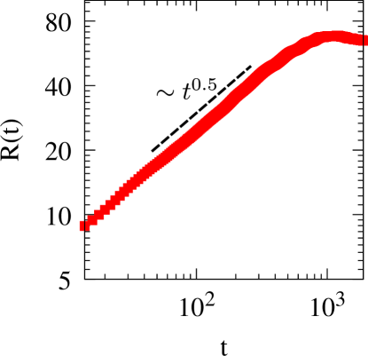
Figure 10: (Color online) $R(t)$ versus $t$ (on a log-log scale) exhibiting a growth exponent $\theta=1/2$ by solving the AIM hydrodynamic equations Eq. (12) and Eq. (13) using the FTCS scheme. Parameters: $L=400$, $\beta=0.75$, and $\rho_{0}=5$.

In Fig. 9, we plot the time evolution of the magnetization field $m$ by solving Eqs. (12) and (13) via the finite difference FTCS scheme. The formation of self-propelling clusters with smooth interfaces and their growth with time resembles the dynamics shown in Fig. 2 for the time-evolution of the microscopic model [Eqs. (1–3)]. We also extract the LCA growth law $R(t)\sim t^{1/2}$ (as shown in Fig. 10 on a logarithmic scale) by solving the hydrodynamic equations after quenching the system from a disordered gaseous phase to an ordered liquid phase. The length scale in Fig. 10 is obtained from the equal-time spatial correlation of the density fields although the length scale obtained from the correlation of the magnetization fields also exhibits the same growth law. Therefore, the self-propulsion terms in the hydrodynamic equations (12) and (13) of the AIM do not affect the asymptotic growth law of the non-conserved Model A.

V Summary and Discussion

We conclude this paper with a summary and discussion of our results. We study the ordering kinetics of the active Ising model (AIM), a flocking model with a non-conserved scalar order parameter, after it is quenched from a disordered high-temperature gaseous phase to the phase-coexistence region and the polar-ordered liquid phase. We observe the formation of connected domains of negative and positive spins similar to the ferromagnetic Ising model in the zero activity diffusive limit of the AIM. But for self-propelled particles, AIM manifests an extensive number of disconnected small clusters of the negative and positive spins which eventually merge to a single, macroscopic liquid domain Solon and Tailleur (2015). The domain evolution morphology is characterized by the equal-time two-point correlation function and its Fourier transform, the structure factor. The scaling of the correlation function exhibits good data collapse, signifying a self-similar nature of the domain growth and the large-$k$ behavior of the scaled structure factor tail shows the Porod’s decay which signifies the smooth spatial structure of the AIM domains. The growth law we extract for the AIM follows the Lifshitz-Cahn-Allen (LCA) growth law Bray (2002, 1994); Puri (2009) $R(t)\sim t^{1/2}$ of the non-conserved scalar order parameter and is unaffected by the system control parameters such as temperature, density, and particle velocity. Unlike the VM Katyal et al. (2020), in AIM, the density domain aligns over the same length scale as the orientation and we do not observe any activity-induced correction to the growth law of non-conserved scalar order parameter discussed in the context of the active polar fluid Dikshit and Mishra (2023). We further investigate the role of diffusion on the AIM growth kinetics. We observe that due to the horizontal biased hopping (along $\pm x$-direction) of the AIM clusters, particle diffusion along the vertical $\pm y$-direction is the predominant mechanism through which coarsening happens in the AIM. This establishes diffusion as the principal growth mechanism rather than activity, leading to a $R(t)\sim t^{1/2}$ growth law for the AIM. We further solve the AIM hydrodynamic equations via a finite difference scheme and the extracted coarsening length scale validates the growth exponent $\theta\simeq 1/2$ observed in the microscopic simulation.

An interesting extension of this study would be to explore the phase ordering kinetics in flocking models in the presence of disorder as experimental systems always contain both quenched and mobile impurities. The similarity in the growth law of a passive system and its active counterpart is an interesting result and therefore, further studies on the coarsening dynamics of active systems, such as the active Potts model or active clock model where the growth law of the corresponding passive models are well-known Grest et al. (1988); Chatterjee et al. (2018, 2020b), are required to confirm (or contradict) this theoretical observation.

VI Acknowledgments

MK acknowledges financial support through a research fellowship from CSIR, Govt. of India (Award Number: 09/080(1106)/2019-EMR-I). RP, SB, AD, and MK thank the Indian Association for the Cultivation of Science (IACS) for its computational facility and resources. SC and HR are financially supported by the German Research Foundation (DFG) within the Collaborative Research Center SFB 1027-A3 and INST 256/539-1. SC acknowledges many helpful discussions with Dr Matthieu Mangeat.

Appendix A Comparison of the growth law for the density and magnetization field

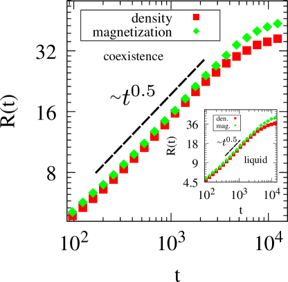
Figure 11: (Color online) $R(t)$ versus $t$ for density and magnetization field yields the same growth exponent 0.5 for a quench in the coexistence regime, $\rho_{0}=3$. (Inset) A similar growth law is extracted for a quench in the liquid regime, $\rho_{0}=10$. Parameters: $L=400$, $\beta=1.1$ and $\epsilon=1$.

The ordering kinetics of the AIM discussed in this paper are studied mainly by extracting the length scale $R(t)$ from the equal-time two-point density correlation function defined in Eq. (4). However, one can also extract $R(t)$ from the magnetization correlation function defined in Eq. (5). Now, it was argued in the context of the coarsening dynamics of the VM that, unlike generic coarsening systems which typically exhibit a single dominant length scale, the Vicsek model exhibits distinct coarsening length scales for the density and velocity correlations Katyal et al. (2020). In VM, despite the density and velocity fields being fully coupled, the velocity length scale grows much faster compared to the density length scale because velocity order extends over longer distances than density clusters due to the irregular fractal morphology of the density clusters. In AIM, however, besides being the density and magnetization fields fully coupled, the clusters are also regularly shaped with smooth boundaries, and therefore, the temporal behavior of the two length scales are found similar as shown in Fig. 11.

Fig. 11 shows, for the coarsening of the AIM, that the two length scales exhibit the same growth law, $R(t)\sim t^{1/2}$ (although the domain size for the density field is marginally larger than the corresponding magnetization field) for a quench into the coexistence region and into the polar ordered liquid regime (see inset of Fig. 11). Therefore, we can conclude that the $R(t)\sim t^{1/2}$ growth law is reasonably universal in the AIM as it neither depends on the quenching regime nor the local order parameter (be it density or magnetization).

Appendix B 2d AIM with $D_{\perp}=0$

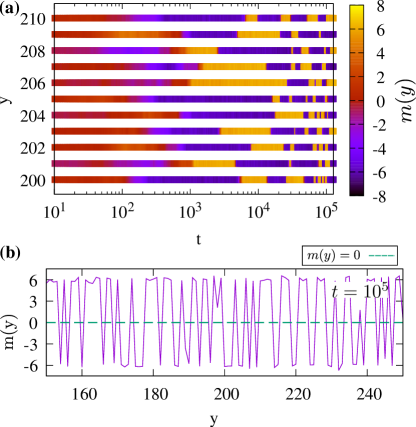
Figure 12: (Color online) (a) $m(y)$ versus $t$ for $L_{y}\in[200:210]$ starting from a random disordered configuration ($m\sim 0$). The color bar denotes the averaged magnetization along the $x$-axis. (b) Late time averaged magnetization profile as a function of $y$. Parameters: $L=400$, $\rho_{0}=10$, $\beta=1.1$, and $\epsilon=0.8$.

The role of transverse diffusion in domain growth of $2d$ AIM is immense. Here we present a more detailed picture of the $D_{\perp}=0$ scenario. In Fig. 12(a) we plot $m(y)=\frac{1}{L_{x}}\sum^{L_{x}}_{i=1}m(i,y)$ versus time $t$ for $L_{y}\in[200:210]$. As the density is very large $(\rho_{0}=10)$, we see highly magnetized one lattice unit-wide domains that can not merge to create a larger domain as time progresses because we inhibit the diffusive hopping in the transverse direction. These $1d$ domains are single dense ordered aggregates that stochastically reverse their magnetization Benvegnen et al. (2022). The magnetization profile in Fig. 12(b) is averaged over $x$ and shows sharp peaks of positive and negative magnetizations, spread over either one site or a few sites. The density profile of such an arrangement shows a homogeneous profile around the average density which is similar to the density profile of a large liquid domain but the alternating magnetization profile signifies that there is no domain growth at the asymptotic limit in the $2d$ AIM for $D_{\perp}=0$.

References

- Ramaswamy (2010) S. Ramaswamy, “The mechanics and statistics of active matter,” Annual Review of Condensed Matter Physics 1, 323–345 (2010).
- Marchetti et al. (2013) M. C. Marchetti, J. F. Joanny, S. Ramaswamy, T. B. Liverpool, J. Prost, M. Rao, and R. A. Simha, “Hydrodynamics of soft active matter,” Reviews of Modern Physics 85, 1143 (2013).
- Needleman and Dogic (2017) D. Needleman and Z. Dogic, “Active matter at the interface between materials science and cell biology,” Nature Reviews Materials 2, 1 (2017).
- Gompper et al. (2020) G. Gompper, R. G Winkler, T. Speck, A. Solon, C. Nardini, F. Peruani, H. Löwen, R. Golestanian, U. B. Kaupp, L. Alvarez, et al., “The 2020 motile active matter roadmap,” Journal of Physics: Condensed Matter 32, 193001 (2020).
- Ballerini et al. (2008) M. Ballerini, N. Cabibbo, R. Candelier, A. Cavagna, E. Cisbani, I. Giardina, V. Lecomte, A. Orlandi, G. Parisi, A. Procaccini, M. Viale, and V. Zdravkovic, “Interaction ruling animal collective behavior depends on topological rather than metric distance: Evidence from a field study,” Proceedings of the National Academy of Sciences 105, 1232 (2008).
- Becco et al. (2006) Ch. Becco, N. Vandewalle, J. Delcourt, and P. Poncin, “Experimental evidences of a structural and dynamical transition in fish school,” Physica A: Statistical Mechanics and its Applications 367, 487–493 (2006).
- Calovi et al. (2014) D. S. Calovi, U. Lopez, S. Ngo, C. Sire, H. Chaté, and G. Theraulaz, “Swarming, schooling, milling: phase diagram of a data-driven fish school model,” New Journal of Physics 16, 015026 (2014).
- Steager et al. (2008) E. B. Steager, C. B. Kim, and M. J. Kim, “Dynamics of pattern formation in bacterial swarms,” Physics of Fluids 20, 073601 (2008).
- Peruani et al. (2012) F. Peruani, J. Starruß, V. Jakovljevic, L. Søgaard-Andersen, A. Deutsch, and M. Bär, “Collective motion and nonequilibrium cluster formation in colonies of gliding bacteria,” Physical Review Letters 108 (2012).
- Schaller et al. (2010) V. Schaller, C. Weber, C. Semmrich, E. Frey, and A. R. Bausch, “Polar patterns of driven filaments,” Nature 467, 73–77 (2010).
- Sumino et al. (2012) Y. Sumino, K. H. Nagai, Y. Shitaka, D. Tanaka, K. Yoshikawa, H. Chaté, and K. Oiwa, “Large-scale vortex lattice emerging from collectively moving microtubules,” Nature 483, 448–452 (2012).
- Sanchez et al. (2012) T. Sanchez, D. T. N. Chen, S. J. DeCamp, M. Heymann, and Z. Dogic, “Spontaneous motion in hierarchically assembled active matter,” Nature 491, 431–434 (2012).
- Vicsek and Zafeiris (2012) T. Vicsek and A. Zafeiris, “Collective motion,” Physics Reports 517, 71–140 (2012).
- Shaebani et al. (2020) M. R. Shaebani, A. Wysocki, R. G. Winkler, G. Gompper, and H. Rieger, “Computational models for active matter,” Nature Reviews Physics 2, 181 (2020).
- De Magistris and Marenduzzo (2015) G. De Magistris and D. Marenduzzo, “An introduction to the physics of active matter,” Physica A: Statistical Mechanics and its Applications 418, 65–77 (2015).
- Krishnan et al. (2010) J. M. Krishnan, A. P. Deshpande, and P. B. S. Kumar, Rheology of complex fluids (Springer, 2010).
- Vicsek et al. (1995) T. Vicsek, A. Czirók, E. Ben-Jacob, I. Cohen, and O. Shochet, “Novel type of phase transition in a system of self-driven particles,” Physical Review Letters 75, 1226 (1995).
- Toner and Tu (1995) J. Toner and Y. Tu, “Long-range order in a two-dimensional dynamical model: How birds fly together,” Physical Review Letters 75, 4326 (1995).
- Toner and Tu (1998) J. Toner and Y. Tu, “Flocks, herds, and schools: A quantitative theory of flocking,” Physical Review E 58, 4828 (1998).
- Solon and Tailleur (2013) A. P. Solon and J. Tailleur, “Revisiting the flocking transition using active spins,” Physical Review Letters 111, 078101 (2013).
- Solon and Tailleur (2015) A. P. Solon and J. Tailleur, “Flocking with discrete symmetry: The two-dimensional active ising model,” Physical Review E 92, 042119 (2015).
- Toner et al. (2005) J. Toner, Y. Tu, and S. Ramaswamy, “Hydrodynamics and phases of flocks,” Annals of Physics 318, 170–244 (2005), special Issue.
- Giomi et al. (2013) L. Giomi, M. J. Bowick, X. Ma, and M. C. Marchetti, “Defect annihilation and proliferation in active nematics,” Physical Review Letters 110, 228101 (2013).
- Cates and Tailleur (2015) M. E. Cates and J. Tailleur, “Motility-induced phase separation,” Annual Review of Condensed Matter Physics 6, 219–244 (2015).
- Solon et al. (2015) A. P. Solon, H. Chaté, and J. Tailleur, “From phase to microphase separation in flocking models: The essential role of nonequilibrium fluctuations,” Physical Review Letters 114, 068101 (2015).
- Siebert et al. (2018) J. T. Siebert, F. Dittrich, F. Schmid, K. Binder, T. Speck, and P. Virnau, “Critical behavior of active brownian particles,” Physical Review E 98, 030601 (2018).
- Wysocki and Rieger (2020) A. Wysocki and H. Rieger, “Capillary action in scalar active matter,” Physical Review Letters 124, 048001 (2020).
- Mangeat et al. (2020) M. Mangeat, S. Chatterjee, R. Paul, and H. Rieger, “Flocking with a -fold discrete symmetry: Band-to-lane transition in the active potts model,” Physical Review E 102, 042601 (2020).
- Chatterjee et al. (2020a) S. Chatterjee, M. Mangeat, R. Paul, and H. Rieger, “Flocking and reorientation transition in the 4-state active potts model,” Europhysics Letters 130, 66001 (2020a).
- Kürsten and Ihle (2020) R. Kürsten and T. Ihle, “Dry active matter exhibits a self-organized cross sea phase,” Physical Review Letters 125, 188003 (2020).
- Fruchart et al. (2021) M. Fruchart, R. Hanai, P. B. Littlewood, and V. Vitelli, “Non-reciprocal phase transitions,” Nature 592, 363 (2021).
- Solon et al. (2022) A. Solon, H. Chaté, J. Toner, and J. Tailleur, “Susceptibility of polar flocks to spatial anisotropy,” Physical Review Letters 128, 208004 (2022).
- Chatterjee et al. (2022) S. Chatterjee, M. Mangeat, and H. Rieger, “Polar flocks with discretized directions: the active clock model approaching the vicsek model,” Europhysics Letters 138, 41001 (2022).
- Codina et al. (2022) J. Codina, B. Mahault, H. Chaté, J. Dobnikar, I. Pagonabarraga, and X. Shi, “Small obstacle in a large polar flock,” Physical Review Letters 128, 218001 (2022).
- Chatterjee et al. (2023) S. Chatterjee, M. Mangeat, C. U. Woo, H. Rieger, and J. D. Noh, “Flocking of two unfriendly species: The two-species vicsek model,” Physical Review E 107, 024607 (2023).
- Karmakar et al. (2023) M. Karmakar, S. Chatterjee, M. Mangeat, H. Rieger, and R. Paul, “Jamming and flocking in the restricted active potts model,” Physical Review E 108, 014604 (2023).
- Bray (2002) A. J. Bray, “Theory of phase-ordering kinetics,” Advances in Physics 51, 481–587 (2002).
- Bray (1994) A. J. Bray, “Theory of phase-ordering kinetics,” Advances in Physics 43, 357 (1994).
- Puri (2009) S. Puri, “Kinetics of phase transitions,” (CRC press, 2009) p. 13.
- Ahmad et al. (2012) S. Ahmad, F. Corberi, S. K. Das, E. Lippiello, S. Puri, and M. Zannetti, “Aging and crossovers in phase-separating fluid mixtures,” Physical Review E 86, 061129 (2012).
- Shrivastav et al. (2014) G. P. Shrivastav, M. Kumar, V. Banerjee, and S. Puri, “Ground-state morphologies in the random-field ising model: Scaling properties and non-porod behavior,” Physical Review E 90, 032140 (2014).
- Kumar et al. (2017) M. Kumar, S. Chatterjee, R. Paul, and S. Puri, “Ordering kinetics in the random-bond XY model,” Physical Review E 96, 042127 (2017).
- Chatterjee et al. (2020b) S. Chatterjee, S. Sutradhar, S. Puri, and R. Paul, “Ordering kinetics in a -state random-bond clock model: Role of vortices and interfaces,” Physical Review E 101, 032128 (2020b).
- Wittkowski et al. (2014) R. Wittkowski, A. Tiribocchi, J. Stenhammar, R. J. Allen, D. Marenduzzo, and M. E. Cates, “Scalar field theory for active-particle phase separation,” Nature Communications 5, 4351 (2014).
- Pattanayak et al. (2021a) S. Pattanayak, S. Mishra, and S. Puri, “Ordering kinetics in the active model B,” Physical Review E 104, 014606 (2021a).
- Pattanayak et al. (2021b) S. Pattanayak, S. Mishra, and S. Puri, “Domain growth in the active model b: Critical and off-critical composition,” Soft Materials 19, 286 (2021b).
- Mishra et al. (2014) S. Mishra, S. Puri, and S. Ramaswamy, “Aspects of the density field in an active nematic,” Philosophical Transactions of the Royal Society A: Mathematical, Physical and Engineering Sciences 372, 20130364 (2014).
- Das et al. (2018) R. Das, S. Mishra, and S. Puri, “Ordering dynamics of self-propelled particles in an inhomogeneous medium,” Europhysics Letters 121, 37002 (2018).
- Saha et al. (2020) S. Saha, J. Agudo-Canalejo, and R. Golestanian, “Scalar active mixtures: The nonreciprocal cahn-hilliard model,” Physical Review X 10, 041009 (2020).
- Rouzaire and Levis (2022) Y. Rouzaire and D. Levis, “Dynamics of topological defects in the noisy kuramoto model in two dimensions,” Frontiers in Physics 10, 976515 (2022).
- Dittrich et al. (2023) F. Dittrich, J. Midya, P. Virnau, and S. K. Das, “Growth and aging in a few phase-separating active matter systems,” Physical Review E 108, 024609 (2023).
- Caporusso et al. (2023) C. B. Caporusso, L. F. Cugliandolo, P. Digregorio, G. Gonnella, D. Levis, and A. Suma, “Dynamics of motility-induced clusters: coarsening beyond ostwald ripening,” Physical Review Letters 131, 068201 (2023).
- Katyal et al. (2020) N. Katyal, S. Dey, D. Das, and S. Puri, “Coarsening dynamics in the vicsek model of active matter,” The European Physical Journal E 43, 10 (2020).
- Dikshit and Mishra (2023) S. Dikshit and S. Mishra, “Ordering kinetics in active polar fluid,” Europhysics Letters 143, 17001 (2023).
- Majumder and Das (2011) S. Majumder and S. K. Das, “Diffusive domain coarsening: Early time dynamics and finite-size effects,” Physical Review E 84, 021110 (2011).
- Chatterjee et al. (2018) S. Chatterjee, S. Puri, and R. Paul, “Ordering kinetics in the -state clock model: Scaling properties and growth laws,” Physical Review E 98, 032109 (2018).
- Dey et al. (2012) S. Dey, D. Das, and R. Rajesh, “Spatial structures and giant number fluctuations in models of active matter,” Physical Review Letters 108, 238001 (2012).
- Yurke et al. (1993) B. Yurke, A. N. Pargellis, T. Kovacs, and D. A. Huse, “Coarsening dynamics of the XY model,” Physical Review E 47, 1525 (1993).
- Benvegnen et al. (2022) B. Benvegnen, H. Chaté, P. L. Krapivsky, J. Tailleur, and A. Solon, “Flocking in one dimension: Asters and reversals,” Physical Review E 106, 054608 (2022).
- Press (2007) W. H. Press, Numerical recipes: The art of scientific computing (Cambridge university press, 2007).
- Grest et al. (1988) G. S. Grest, M. P. Anderson, and D. J. Srolovitz, “Domain-growth kinetics for the Q-state potts model in two and three dimensions,” Physical Review B 38, 4752 (1988).