Generating random Gaussian states

Abstract.

We develop a method for the random sampling of (multimode) Gaussian states in terms of their covariance matrix, which we refer to as a random quantum covariance matrix (RQCM). We analyze the distribution of marginals and demonstrate that the eigenvalues of an RQCM converge to a shifted semicircular distribution in the limit of a large number of modes. We provide insights into the entanglement of such states based on the positive partial transpose (PPT) criteria. Additionally, we show that the symplectic eigenvalues of an RQCM converge to a probability distribution that can be characterized using free probability. We present numerical estimates for the probability of a RQCM being separable and, if not, its extendibility degree, for various parameter values and mode bipartitions.

Keywords. Gaussian state, random matrices, extendability, entanglement, PPT criterion, symplectic eigenvalues.

Mathematics Subject Classification (2010): 81P40, 81P99, 94A15.

1. Introduction

Quantum mechanics can be considered as a non-commutative version of classical probability theory [Mac63, Par92, Mey93, Par05]. However most often in quantum information theory, probability theory was used in the areas which rely on the measurement statistics. The trend changed with the seminal paper of Hayden et al [HLW06] which used random matrix and concentration of measure techniques in quantum information theory. Henceforth, random matrix techniques have been used extensively in this area. For construction of random states, see the paper of Życzkowski et al [ŻPNC11], and the review article [CN16].

Continuous variable quantum systems are one of the most useful systems for the quantum information processing. Among these, Gaussian states play a crucial role. Gaussian states and their applications are studied extensively in the literature. These concepts, explained from a mathematical point can been seen in the book of Holevo [Hol11]. Gaussian states are easy to prepare, manipulate, or measure and have wide range of applications in quantum optics and quantum communications [WPGP⁺12, ARL14].

There are very few works on using random matrix techniques and Gaussian states. The only attempt as per our knowledge if the work of Serafini et al [SDGP07] which was further developed by Fukuda and König [FK19]. In these papers, the authors introduced a method to generate the random Gaussian states. The novelty of the present work is that it uses a different method of sampling. Furthermore, this also explores the problem of entanglement detection for such states.

Gaussian states can be represented by their covariance matrices which are real positive definite matrices satisfying a Heisenberg-type uncertainty relation. This is the point of view we adopt in this work for sampling Gaussian states. We are going to modify a well-known ensemble of real random matrices (the Gaussian Orthogonal Ensemble - GOE) in order to impose the uncertainty condition.

Recall that an element of the GOE is a real symmetric random matrix, with Gaussian entries that are independent (up to the symmetry condition). Wigner [Wig55] famously showed that the eigenvalues of GOE random matrices converge to the semicircle distribution (see Figure 2). In particular, this means that GOE matrices are likely to have negative eigenvalues, so they cannot be covariance matrices of Gaussian quantum states. In order to fulfill the uncertainty principle, we shall uniformly shift the GOE element by the minimal amount needed to satisfy the uncertainty principle. We introduce in this way the ensemble of random matrices that we shall study:

Definition.

A random quantum covariance matrix (RQCM) is defined by

$$S_{G}:=G+\lambda_{\max}(\mathrm{i}J_{2n}-G)\cdot I_{2n},$$

where $G$ is a GOE random matrix and $J_{2n}=\big{[}\begin{smallmatrix}0&1\\ -1&0\end{smallmatrix}\big{]}^{\oplus n}$.

Note that one can choose freely the variance of the elements of the GOE ensemble, so in this way we obtain a one-parameter family of probability distributions on random quantum covariance matrices; we refer the reader to Definition 3.2 for the precise statements.

The rest of the paper is devoted to the study of this ensemble, with a focus on entanglement properties of random Gaussian states on $m+n$ modes. In particular, we show that:

• the choice of shifting a given matrix to enforce the Heisenberg uncertainty relation is motivated by an optimization problem related to the operator norm (Section 3.1)

• the distribution of the $m$-mode marginal of a $(m+n)$-mode RQCM is part of the same ensemble of distributions (3.2 and 4.3)

• the eigenvalues of a RQCM converge, in the large number of modes limit, to a shifted semicircular distribution (Theorem 4.1)

• RQCMs (almost) satisfy the positive partial transposition (PPT) criterion, in the same asymptotic regime (Theorem 4.2)

• the purity of a RQCM decreases exponentially with the number of modes (4.2)

• the symplectic eigenvalues of a RQCM converge to a probability distribution that can be characterized using free probability (Theorem 5.1)

• RQCM states have very interesting entanglement and extendability properties, that we probe numerically in Section 6, in different scenarios corresponding to several bipartitions of the number of modes and the variance parameter of the RQCM distribution.

The results described above encapsulate most of the important properties of random Gaussian states. We argue that the ensemble of quantum covariance matrices that we introduced is natural, both from a physical perspective (it is invariant with respect to the action of the ortho-symplectic group) and from a mathematical perspective. Importantly, we relate the study of their properties to free probability theory [VDN92, NS06, MS17].

Let us note that there has been earlier work on random Gaussian quantum states [Ser17, FK19]. Importantly, in the latter work, the authors take a completely different approach: they fix a set of symplectic eigenvalues, then they generate a random pure Gaussian state by randomly rotating the diagonal symplectic matrix, and finally they take the partial trace to obtain a general Gaussian state. In [FK19], the major hurdle is the fact that the group

$$\mathsf{Sp}(2n,\mathbb{R})=\{L\in M(2n,\mathbb{R}):LJ_{2n}L^{t}=J_{2n}\},$$

which is the symmetry group for pure Gaussian states, is not compact; hence sampling on this group is difficult. This approach is fundamentally different than ours: we construct directly the mixed quantum states, bypassing the pure states, for which there is no canonical invariant probability distribution. Our goal is to study different properties of typical Gaussian states by using random matrix theory. The key part in this work is the novel sampling technique which will be discussed in Section 3. In Sections 4, 5, 6 we study different spectral and entanglement properties of the newly introduced ensemble, using various techniques from random matrix theory and free probability theory. The results are presented in such a way that one can use them readily to perform analytical computations and numerical simulations for problems involving Gaussian states described by covariance matrices. Hence, we hope that our work provides a useful toolbox for researchers investigating entanglement properties of such quantum states, similarly to previous investigations in the discrete setting [ŻPNC11, KNP⁺21].

The paper is organized as follows. In Section 2, we are giving a short introduction of Gaussian states and entanglement, which will be used later in the paper. In Section 3.1 we justify our approach to defining random quantum covariance matrices by showing that our method is equivalent to picking the closest (in operator norm) quantum covariance matrix to a GOE element. In the rest of Section 3 we introduce random quantum covariance matrices and study their most basic properties. Sections 4 and 5 deal with properties related to usual and symplectic eigenvalues in the large number of modes asymptotic limit. Finally, Section 6, more numerical in nature, gathers results about the entanglement of typical quantum covariance matrices.

A Mathematica notebook containing numerical routines to sample random quantum covariance matrices and to test important entanglement-related properties is available at [LNS24].

2. Gaussian states and their entanglement

A quantum state is a positive semidefinite trace class operator with trace 1, in a separable complex Hilbert space. Consider the ‘$n$-mode’ Fock space $\Gamma(\mathbb{C}^{n})$. A Gaussian state $\rho$ acting on this space is a state such that its expectation with respect to the position or momentum operator in any mode gives a classical Gaussian distribution. In this work, we plan to explore properties of Gaussian states.

A state $\rho$ in $\Gamma(\mathcal{H})$ with a Hilbert space $\mathcal{H}=\mathbb{C}^{n}$ is an $n$-mode Gaussian state if its Fourier transform $\hat{\rho}$ is given by

$$\hat{\rho}(\bm{x}+\imath\bm{y})=\exp\left[-\imath\sqrt{2}(\bm{l}^{T}\bm{x}-\bm{m}^{T}\bm{y})-\frac{1}{2}\left[\tau\begin{pmatrix}\bm{x}\\ \bm{y}\end{pmatrix}\right]^{T}S\left[\tau\begin{pmatrix}\bm{x}\\ \bm{y}\end{pmatrix}\right]\right].$$ (2.1)

for all $\bm{x},~{}\bm{y}\in\mathbb{R}^{n}$ where $\bm{l},~{}\bm{m}$ are the momentum-position mean vectors and $S/2$ their covariance matrix. $\tau:\mathbb{R}^{2n}\rightarrow\mathbb{R}^{2n}$ is given by $\tau(x_{1},\cdots,x_{n},y_{1},\cdots,y_{n})^{T}=(x_{1},y_{1},\cdots,x_{n},y_{n})^{T}$ [Par10].

If $\rho$ is a state of a quantum system and $X_{i},\,i=1,2$ are two real-valued observables, or equivalently, self-adjoint operators with finite second moments in the state $\rho$ then the covariance between $X_{1}$ and $X_{2}$ in the state $\rho$ is the scalar quantity

$$\mathrm{Tr\,}\left(\frac{1}{2}(X_{1}X_{2}+X_{2}X_{1})\rho\right)-\left(\mathrm{Tr\,}X_{1}\rho\right)\cdot\left(\mathrm{Tr\,}X_{2}\rho\right),$$

which is denoted by $\mathrm{Cov}_{\rho}(X_{1},X_{2})$. Suppose $q_{1},p_{1};\,q_{2},p_{2};\,\cdots;\,q_{n},p_{n}$ are the position - momentum pairs of observables of a quantum system with $n$ degrees of freedom obeying the canonical commutation relations. Then we express

$$(X_{1},X_{2},\cdots,X_{2n})=(q_{1},-p_{1},q_{2},-p_{2},\cdots,q_{n},-p_{n}).$$

If $\rho$ is a state in which all the $X_{j}$’s have finite second moments we write

$$S_{\rho}=\Big{[}\mathrm{Cov}_{\rho}(X_{i},X_{j})\Big{]}_{i,j=1}^{2n}.$$ (2.2)

We call $S_{\rho}$ the covariance matrix of the position momentum observables. If we write

$$J_{2n}=\begin{bmatrix}\begin{array}[]{rr}0&1\\ -1&0\end{array}&&&\\ &\begin{array}[]{rr}0&1\\ -1&0\end{array}&&\\ &&\ddots&\\ &&&\begin{array}[]{rr}0&1\\ -1&0\end{array}\end{bmatrix}=\begin{bmatrix}0&1\\ -1&0\end{bmatrix}\otimes I_{n}$$ (2.3)

where $I_{n}$ is the identity matrix of order $n$; or equivalently we may write it as $\big{[}\begin{smallmatrix}0&1\\ -1&0\end{smallmatrix}\big{]}^{\oplus n}$ for the $2n\times 2n$ block diagonal matrix, the complete Heisenberg uncertainty relations for all the position and momentum observables assume the form of the following matrix inequality

$$S_{\rho}+\mathrm{i}J_{2n}\geq 0.$$ (2.4)

Conversely, if $S$ is any real $2n\times 2n$ symmetric matrix obeying the inequality $S+\mathrm{i}J_{2n}\geq 0$, then there exists a state $\rho$ such that $S$ is the covariance matrix $S_{\rho}$ of the observables $q_{1},-p_{1};\,q_{2},-p_{2};\,\cdots;\,q_{n},-p_{n}$. In such a case $\rho$ can be chosen to be a Gaussian state with mean zero. For a $n$-mode covariance matrix $S$ the positive eigenvalues of the matrix $\mathrm{i}J_{2n}S$ are called the symplectic eigenvalues of $S$.

The importance of finite mode Gaussian states and their covariance matrices in general quantum theory as well as quantum information has been highlighted extensively in the literature. A comprehensive survey of Gaussian states and their properties can be found in the book of Holevo [Hol11]. For their applications to quantum information theory the reader is referred to the survey article by Weedbrook et al [WPGP⁺12] as well as Holevo’s book [Hol12]. For our reference we use [ADMS95, Par10, Par13] for Gaussian states. For notations in the following sections we use [PS15b] and [PS15a].

2.1. Entanglement of Gaussian states

One of the most important problems in quantum mechanics as well as quantum information theory is to determine whether a given bipartite state is separable or entangled [NC10]. There are several methods in tackling this problem leading to a long list of important publications. A detailed discussion on this topic is available in the survey articles by Horodecki et al [HHHH09], and Gühne and Tóth [GT09]. One such condition which is both necessary and sufficient for separability in finite dimensional product spaces is complete extendability [DPS04]. Let us denote by $\mathcal{B(H)}$ the set of bounded operators on a Hilber space $\mathcal{H}$.

Definition 2.1.

Let $k\in\mathbb{N}$. A state $\rho\in\mathcal{B}(\mathcal{H}_{A}\otimes\mathcal{H}_{B})$ is said to be $k$-extendable with respect to system $B$ if there is a state $\tilde{\rho}\in\mathcal{B}(\mathcal{H}_{A}\otimes\mathcal{H}_{B}^{\otimes k})$ which is invariant under any permutation in $\mathcal{H}_{B}^{\otimes k}$ and $\rho=\mathrm{Tr\,}_{\mathcal{H}_{B}^{\otimes(k-1)}}\tilde{\rho}$, $k\geq 2$.

A state $\rho\in\mathcal{B}(\mathcal{H}_{A}\otimes\mathcal{H}_{B})$ is said to be completely extendable if it is $k$-extendable for all $k\in\mathbb{N}$.

The following theorem of Doherty, Parrilo, and Spedalieri [DPS04] emphasizes the importance of the notion of complete extendability.

Theorem A.

[DPS04] A bipartite state $\rho\in\mathcal{B}(\mathcal{H}_{A}\otimes\mathcal{H}_{B})$ is separable if and only if it is completely extendable with respect to one of its subsystems.

It is fairly simple to see that separability implies complete extendability. The proof of the converse depends on an application of the quantum de Finetti theorem [Stø69, HM76], according to which any exchangable state is, indeed, separable. The link between separability and extendability has found applications in quantum information theory [BCY11, BH13]. Here we study the same in the context of quantum Gaussian states.

This proof directly follows from work of Hudson and Moody [HM76]. The problem of finding necessary and sufficient conditions for $k$-extendability of non-Gaussian states is open.

Definition 2.2 (Gaussian extendability).

Let $k\in\mathbb{N}$. A Gaussian state $\rho_{g}$ in $\Gamma(\mathbb{C}^{m})\otimes\Gamma(\mathbb{C}^{n})$ is said to be Gaussian $k$-extendable with respect to the second system if there is a Gaussian state $\tilde{\rho_{g}}$ in $\Gamma(\mathbb{C}^{m})\otimes\Gamma(\mathbb{C}^{n})^{\otimes k}$ which is invariant under any permutation in $\Gamma(\mathbb{C}^{n})^{\otimes k}$ and $\rho_{g}=\mathrm{Tr\,}_{\Gamma(\mathbb{C}^{n})^{\otimes(k-1)}}\tilde{\rho_{g}}$, $k\geq 2$.

A Gaussian state $\rho_{g}$ in $\Gamma(\mathbb{C}^{m})\otimes\Gamma(\mathbb{C}^{n})$ is said to be Gaussian completely extendable if it is Gaussian $k$-extendable for every $k\in\mathbb{N}$.

Entanglement property of a Gaussian state depends only on its covariance matrix. Hence without loss of generality, we can confine our attention to the Gaussian states with mean zero. Thus an $(m+n)$-mode mean zero Gaussian state in $\Gamma(\mathbb{C}^{m})\otimes\Gamma(\mathbb{C}^{n})$ is uniquely determined by a $2(m+n)\times 2(m+n)$ covariance matrix

$$S=\begin{bmatrix}A&B\\ B^{T}&C\end{bmatrix}.$$ (2.5)

In this paper, we shall call the matrices above quantum covariance matrices, following the terminology from [LRW⁺18]. Here $A$ and $C$ are covariance matrices of the $m$ and $n$-mode marginal states respectively.

If $\rho(\bm{0},\bm{0};S)$, written in short as $\rho(S)$ in $\Gamma(\mathbb{C}^{m})\otimes\Gamma(\mathbb{C}^{n})$ is $k$-extendable with respect to the second system, then there exists a real matrix $\theta_{k}$ of order $2n\times 2n$ such that the extended matrix

$$S_{k}=\left[\begin{array}[]{c|cccc}A&B&B&\cdots&B\\ \hline\cr B^{T}&C&\theta_{k}&\cdots&\theta_{k}\\ B^{T}&\theta_{k}^{T}&C&\cdots&\theta_{k}\\ \vdots&\vdots&\vdots&\ddots&\vdots\\ B^{T}&\theta_{k}^{T}&\theta_{k}^{T}&\cdots&C\end{array}\right]$$ (2.6)

is the covariance matrix of a Gaussian state in $\Gamma(\mathbb{C}^{m})\otimes\Gamma(\mathbb{C}^{n})^{\otimes k}$. Then it satisfies inequality (2.4) in the form

$$S_{k}+\mathrm{i}J_{2(m+kn)}\geq 0.$$ (2.7)

Theorem B.

[BPS17] Let $\rho$ be a bipartite Gaussian state in $\Gamma(\mathbb{C}^{m})\otimes\Gamma(\mathbb{C}^{n})$ with covariance matrix $S=\begin{bmatrix}A&B\\ B^{T}&C\end{bmatrix}$, where $A$ and $C$ are marginal covariance matrices of the first and second system respectively. Then $\rho$ is completely extendable with respect to the second system if and only if there exists a real positive matrix $\theta$ such that

$$C+\mathrm{i}J_{2n}\geq\theta\geq B^{T}\left(A+\mathrm{i}J_{2m}\right)^{-}B,$$ (2.8)

where $\left(A+\mathrm{i}J_{2m}\right)^{-}$ is the Moore-Penrose inverse of $A+\mathrm{i}J_{2m}$.

From this the following result can be constructed.

Theorem C.

Any separable Gaussian state in a bipartite system is completely extendable and conversely every completely extendable Gaussian state is separable.

The authors of the paper [BPS17] have shown that the result in C is true for any state (need not be Gaussian) in bipartite Fock space as well. However it may not be possible to get any analogous matrix inequality as entanglement in such systems is more completed than the finite dimensional versions. Later Lami et al [LKAW19] gave an improved version of the B where they gave explicit bounds for the different level of entanglement. The result is as follows.

Theorem D.

Let $\rho_{AB}$ be a $k$-extendible (not necessarily Gaussian) state of $m+n$ modes with covariance matrix $S$. Then there exists a $2n\times 2n$ quantum covariance matrix $\Delta\geq\mathrm{i}J_{2n}$ for the space $B$ such that

$$S\geq\mathrm{i}J_{2m}\oplus\left[\left(1-\frac{1}{k}\right)\Delta+\frac{1}{k}\mathrm{i}J_{2n}\right].$$ (2.9)

Moreover, the above condition is necessary and sufficient for $k$-extendibility when $\rho_{AB}$ is Gaussian. In this case the equation (2.9) can further be simplified as

$$\mathrm{i}J_{2n}\leq\Delta\leq\frac{k}{k-1}\left[C-B^{T}(A-\mathrm{i}J_{2m})^{-1}B\right]-\frac{1}{k-1}\mathrm{i}J_{2n}.$$ (2.10)

Furthermore, if $\rho_{AB}$ is an $m+n$ mode $k$-extendible Gaussian state, then

$$\|\rho_{AB}-\mathrm{SEP}(m,l)\|_{1}\leq 2n/k,$$ (2.11)

where $\mathrm{SEP}(m,n)$ is the set of bipartite separable states of the systems of $m$ and $n$ modes and $||\cdot||_{1}$ is the trace norm.

Both the complete extendability and $k$-compatibility criteria can be cast as semidefinite programs (SDPs). While one can in principle determine the separability of any covariance matrix by running the SDPs, for sufficiently large matrices solving the SDPs might become cumbersome because of the excessive run-time. However, there are also other, perhaps simpler, entanglement criteria. One of the most well-known is the positive partial transpose (PPT) criteria. The PPT criteria of Gaussian states can be expressed in the following way. Consider a $(m+n)$-mode Gaussian state with covariance matrix $S$ as given in the Theorem C. It naturally satisfies the equation (2.3) with appropriate dimension. It is considered a PPT state if

$$S+\mathrm{i}\begin{bmatrix}J_{2m}&\\ &-J_{2n}\end{bmatrix}\geq 0.$$ (2.12)

Simon [Sim00] showed that a 2-mode Gaussian state is separable if and only if its covariance matrix $S$ satisfies (2.12). Furthermore it has been proven that this also holds for any $(n+1)$-mode Gaussian state where the bipartition is taken as in the $n$-mode vs 1-mode way. However, in general the PPT condition is not necessary and sufficient for separability. In fact, Werner and Wolf [WW01] constructed examples of Gaussian states on 2-mode $\times$ 2-modes settings which satisfies (2.12) but is entangled.

2.2. Previous work on random Gaussian states

Here we give the two different methods of sampling given in Fukuda and König [FK19] using techniques proposed earlier by Serafini et al [SDGP07].

Consider the system $\mathcal{H}_{A}\otimes\mathcal{H}_{B}=L^{2}(\mathbb{R})^{\otimes k}\otimes L^{2}(\mathbb{R})^{\otimes(n-k)}$, where the system is of $k$-modes with $(n-k)$-modes of environment. Consider a pure Gaussian state $\ket{\Phi}\in\mathcal{H}_{A}\otimes\mathcal{H}_{B}$ bounded by the compactness criteria (i.e. energy constrain)

$$\langle\Phi|H_{AB}|\Phi\rangle\leq E,$$

with the Hamiltonian

$$H_{AB}=\sum_{j=1}^{n}(Q_{j}^{2}+P_{j}^{2}).$$

This can be diagonalised by passive way, i.e. by using the ortho-symplectic group $\mathsf{K}(2n):=\mathsf{Sp}(2n)\cap\mathsf{O}(2n)$ we can write this as the diagonal matrix $\hat{Z_{n}}=Z_{n}\oplus Z_{n}^{-1}$ where $Z_{n}=\operatorname{diag}(z_{1},\cdots,z_{n})$, with $z_{j}\geq 1$ for all $j$, and

$$\sum_{j=1}^{n}\left(z_{j}+\frac{1}{z_{j}}\right)\leq E.$$

The left hand side is actually the energy $\langle\Phi|H_{AB}|\Phi\rangle$ of the state $\ket{\Phi}$. The method can be expressed as fellows. First to choose $z_{j}$’s randomly with required properties and bounds, which in turn gives a pure state in the state space. After this we may apply a random ortho-symplectic transformation. This is allowed as the group $\mathsf{K}(2n)$ is compact. Following this we may remove the extra $(n-k)$ modes associated with environment by using partial trace to generate a $k$-mode random mixed Gaussian state.

Previously, Serafini et al [SDGP07] considered the two following measured based on the above protocol.

Microcanonical measure $\mu_{micro}$:

This is done by first drawing $(E_{1},\cdots,E_{n})$ uniformly (according to the measure induced by the Lebesgue measure on $\mathbb{R}^{n}$) from the set

$$\Gamma_{E}=\left\{(E_{1},\cdots,E_{n}):E_{j}\geq 2~{}\forall j,~{}\sum_{j=1}^{n}E_{j}\leq E\right\}.$$

Then

$$z_{j}=\frac{1}{2}(E_{j}+\sqrt{E_{j}^{2}-4}),$$

for $j=1,\cdots,n$ and drawing pure states from $\mu_{micro}$.

Canonical measure $\mu_{canonical}$:

This is achieved by drawing $E=(E_{1},\cdots,E_{n})$ based on Boltzmann distribution

$$\mathrm{d}p(E)=\frac{1}{T^{n}}\exp\left[-\frac{1}{T}\left(\sum_{j=1}^{n}E_{j}-2n\right)\right]\mathrm{d}E_{1}\cdots\mathrm{d}E_{n}$$

with temperature $T=\frac{E}{n}$ and setting

$$z_{j}=\frac{1}{2}(E_{j}+\sqrt{E_{j}-4})$$

for $j=1,\cdots,n$ and drawing pure states.

3. Random quantum covariance matrices

In this section, we shall introduce a random matrix ensemble of Gaussian covariance matrices. Our inspiration comes from the discrete case, where such ensembles of random density matrices have found many applications in quantum information theory and beyond. Ensembles of (finite dimensional) density matrices [Bra96, Hal98, ŻS01, SŻ04, ŻPNC11] have been studied thoroughly in relation to many topics such as quantum entanglement or quantum chaos. Ensembles of quantum channels have been successfully used to prove many important results in quantum information theory [HLW06, Has09]; see [CN16] for a review of these topics.

Recall that a Gaussian covariance matrix is a real symmetric matrix $S\in\mathcal{M}_{2n}(\mathbb{R})$ satisfying the condition

$$S\geq\mathrm{i}J_{2n}.$$

Mathematically, the condition above is interesting since it requires a complex positive semidefiniteness condition of a real object. A random quantum covariance matrix will be defined to be an element of the Gaussian Orthogonal Ensemble (GOE) shifted by a multiple of the identity matrix in order for the condition $S\geq\mathrm{i}J_{2n}$ to be satisfied. Our approach is motivated by the following two independent facts:

• the ensemble of random quantum covariance matrices we construct has is invariant under the ortho-symplectic group $\mathsf{K}(2n)=\mathsf{Sp}(2n)\cap\mathsf{O}(2n)$, see 3.1;

• to a GOE element $G$, we associate the closest (in operator norm) quantum covariance matrix $H$, see Section 3.1.

We start by investigating the problem of finding the closes quantum covariance matrix to a given matrix. After recalling some basic facts about GOE random matrices, we introduce the ensemble of random quantum covariance matrices (RQCM) along with some of its basic properties. Later, in Section 4 we study the large $n$ limit of this ensemble.

3.1. Closest quantum covariance matrix

Consider an arbitrary real symmetric matrix $G\in\mathcal{M}_{2n}^{sa}(\mathbb{R})$. We are interested in finding the closest quantum covariance matrix to $G$, that is

$$\min \quad\|G-H\|$$

s.t. $$\quad H\in\mathcal{M}_{2n}^{sa}(\mathbb{R})$$ (3.1)

$$\quad H\geq\mathrm{i}J_{2n},$$

where $\mathcal{M}^{sa}_{2n}(\mathbb{R})$ denotes the set of $2n\times 2n$ real and self-adjoint, i.e., symmetric matrices.

The geometry of the optimization problem above depends on the norm used as a cost function. We consider here the operator norm $\|\cdot\|_{\infty}$. The optimization problem (3.1) becomes an SDP:

$$\min \quad t$$

s.t. $$\quad H\in\mathcal{M}_{2n}^{sa}(\mathbb{R}),t\in\mathbb{R}$$

$$\quad H\geq\mathrm{i}J_{2n}$$

$$\quad-tI_{2n}\leq G-H\leq tI_{2n}.$$

The dual SDP can be easily computed:

$$\max \quad\langle Z,iJ_{2n}-G\rangle$$

s.t. $$\quad Z\in\mathcal{M}_{2n}^{sa}(\mathbb{C})$$ (3.2)

$$\quad Z\geq 0$$

$$\quad\|\operatorname{Re}Z\|_{1}\leq 1.$$

However, since $Z\geq 0$, we also have $\operatorname{Re}Z\geq 0$ and thus the last condition above reads simply $\operatorname{Tr}Z\leq 1$, yielding the explicit solution

$$\lambda(G)=\max(0,\lambda_{\max}(\mathrm{i}J_{2n}-G)).$$ (3.3)

In particular, we see that in the case when $G\geq\mathrm{i}J_{2n}$, one can simply take $H=G$, obtaining the optimum 0.

Importantly, there is a trivial solution $H=G+\lambda(G)I_{2n}$ achieving the value above. Indeed, write the decomposition of the matrix $G-\mathrm{i}J_{2n}$ into its positive and negative parts:

$$G-\mathrm{i}J_{2n}=A-B,$$

with $A,B\geq 0$ having orthogonal supports. Clearly, $\lambda(G)=\lambda_{\max}(B)\geq 0$, and we have

$$G+\lambda_{\max}(B)I_{2n}=\mathrm{i}J_{2n}+A+(\lambda_{max}(B)I_{2n}-B)\geq\mathrm{i}J_{2n},$$

proving that $G+\lambda_{\max}(B)I_{2n}$ achieves the optimum value in the primal program. The geomtry of the problem and the closest matrix $H$ described above are presented graphically in Figure 1.

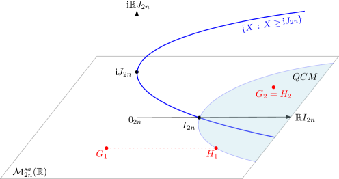
Figure 1. Finding the closest (in operator norm) quantum covariance matrix $H$ to a given real symmetric matrix $G$. We display two examples: $G_{1}$ is not a quantum covariance matrix, so it needs to be shifted by a multiple of the identity matrix to become one ($H_{1}$); $G_{2}$ is already a quantum covariance matrix, so $H_{2}=G_{2}$.

3.2. Basic properties of GOE matrices

The Gaussian orthogonal ensemble $\mathrm{GOE}$ is arguably the most studied ensemble of random matrices. It consists of real symmetric matrices distributed along the Gaussian distribution on the corresponding vector space.

Definition 3.1.

A random symmetric matrix $G\in\mathcal{M}^{sa}_{n}(\mathbb{R})$ is said to have a $\mathrm{GOE}(n,\sigma)$ distribution if:

• the random variables $\{G_{ij}\}_{1\leq i\leq j\leq n}$ are independent;

• the diagonal entries have distribution

  $$\forall i\in[n],\qquad G_{ii}\sim\mathcal{N}(0,2\sigma^{2})$$

• the off-diagonal entries have distribution

  $$\forall i<j\in[n],\qquad G_{ij}=G_{ji}\sim\mathcal{N}(0,\sigma^{2}).$$

On the space of real symmetric matrices, random $\mathrm{GOE}(n,\sigma=1)$ matrices have distribution given by [AGZ10, Section 2.5.1]

$$\frac{\mathrm{d}G}{\mathrm{d}\mathrm{Leb}}=2^{-n/2}(2\pi)^{-n(n+1)/4}\exp\big{(}-\operatorname{Tr}(G^{2})/4\big{)},$$

where $\mathrm{Leb}$ is the Lebesgue measure on the vector space of $n\times n$ real symmetric matrices.

Wigner famously showed that the empirical eigenvalue distribution

$$\mu_{G}:=\frac{1}{n}\sum_{i=1}^{n}\delta_{\lambda_{i}(G)}$$

converges to the (centered) semicircle distribution defined by

$$\mathrm{d}\mathrm{SC}_{\sigma}=\frac{\sqrt{4\sigma^{2}-x^{2}}}{2\pi\sigma^{2}}\mathbf{1}_{|x|\leq 2\sigma}(x)\mathrm{d}x.$$

Theorem 3.1.

[Wig55] Let $\sigma>0$ and $G_{n}\sim\mathrm{GOE}(n,\sigma)$ be a sequence of $\mathrm{GOE}$ random matrices. Then, almost surely,

$$\lim_{n\to\infty}\mu_{G_{n}/\sqrt{n}}=\mathrm{SC}_{\sigma},$$

where the convergence of probability measures is considered in the weak sense.

We plot in Figure 2 the empirical histogram of eigenvalues versus the theoretical curve of the semicircular distribution. Note also that the largest and the smallest eigenvalues of a $\mathrm{GOE}$ matrix also converge to the edges of the support of the semicircular distribution.

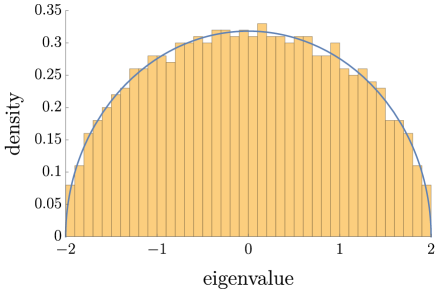
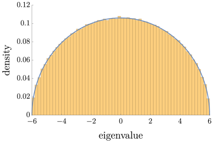
Figure 2. Theoretical curve (blue) and histogram of eigenvalues of one realization of $\mathrm{GOE}$ matrices (yellow). Left: $n=500$, $\sigma=1$; right: $n=5000$, $\sigma=3$.

Theorem 3.2.

[FK81] Let $\sigma>0$ and $G_{n}\sim\mathrm{GOE}(n,\sigma)$ be a sequence of $\mathrm{GOE}$ random matrices. Then, almost surely,

$$\lim_{n\to\infty}\lambda_{\min}(G_{n}/\sqrt{n})=-2\sigma\quad\text{ and }\quad\lim_{n\to\infty}\lambda_{\max}(G_{n}/\sqrt{n})=2\sigma.$$

3.3. Random Quantum Covariance Matrices — RQCM

As motivated at the beginning of the section, we shall define the ensemble of random quantum covariance matrices associating to an element $G$ of the GOE ensemble the closest quantum covariance matrix, see Eq. 3.1. Note however that if $G$ is already a quantum covariance matrix, we still shift $G$ by a multiple of the identity.

Definition 3.2.

For a given $n\geq 1$, let $G\in\mathrm{GOE}(2n,\sigma)$ be an element of the Gaussian Orthogonal Ensemble with mean $0$ and variance $\sigma^{2}$. A random quantum covariance matrix of parameter $\sigma$ is a matrix

$$S_{G}:=G+\lambda_{\max}(\mathrm{i}J_{2n}-G)\cdot I_{2n}.$$

We denote by $\mathrm{RQCM}(2n,\sigma)$ the ensemble of such random matrices.

Clearly, every element of $\mathrm{RQCM}(2n,\sigma)$ is a Gaussian covariance matrix:

$$\lambda_{\min}(S_{G}-\mathrm{i}J_{2n})=\lambda_{\min}(G-\mathrm{i}J_{2n})+\lambda_{\max}(\mathrm{i}J_{2n}-G)=0.$$

The $\mathrm{RQCM}$ ensemble has $\mathsf{K}(2n)=\mathsf{O}(2n)\cap\mathsf{Sp}(2n)$ symmetry, as it is shown in the following proposition.

Proposition 3.1.

For any real matrix $G\in\mathcal{M}_{2n}(\mathbb{R})$ and any operator $U\in\mathsf{K}(2n)$, we have

$$S_{UGU^{\top}}=US_{G}U^{\top}.$$

In particular, if $S$ is a random matrix having $\mathrm{RQCM}(2n,\sigma)$ distribution, then so does $UGU^{\top}$. In other words, the ensemble $\mathrm{RQCM}(2n,\sigma)$ is invariant with respect to the ortho-symplectic group.

Proof.

Compute

$$S_{UGU^{\top}} =UGU^{\top}+\lambda_{\max}(\mathrm{i}J_{2n}-UGU^{\top})I_{2n}$$

$$=UGU^{\top}+\lambda_{\max}\bigg{(}U(\mathrm{i}\underbrace{U^{\top}J_{2n}U}_{J_{2n}}-G)U^{\top}\bigg{)}I_{2n}$$

$$=UGU^{\top}+\lambda_{\max}(\mathrm{i}J_{2n}-G)I_{2n}$$

$$=U\bigg{(}G+\lambda_{\max}(\mathrm{i}J_{2n}-G)I_{2n}\bigg{)}U^{\top}$$

$$=US_{G}U^{\top}.$$

For the second claim, if $S$ has $\mathrm{RQCM}(2n,\sigma)$ distribution, then $S=S_{G}$ for a random matrix $G$ having $\mathrm{GOE}(2n,\sigma)$ distribution. It follows that $UGU^{\top}$ also has $\mathrm{GOE}(2n,\sigma)$ distribution, and thus $USU^{\top}=US_{G}U^{\top}=S_{UGU^{\top}}$ has $\mathrm{RQCM}(2n,\sigma)$ distribution. ∎

Let us consider now the partial trace operator, where, given a Gaussian covariance matrix $S\in\mathcal{M}_{2n}(\mathbb{R})$ corresponding to a $n$-mode Gaussian state, we associate its $m$-mode marginal $S^{(2m)}$, obtained as its top-left $2m\times 2m$ block, see Eq. (2.5). The following result shows that the $\mathrm{RQCM}$ ensemble is, up to translations, stable under taking marginals.

Proposition 3.2.

Let $S$ be a random quantum covariance matrix having $\mathrm{RQCM}(2n,\sigma)$ distribution, and let $1\leq m<n$. Then, its $m$-mode marginal has a shifted $\mathrm{RQCM}(2m,\sigma)$ distribution.

Proof.

Writing $S=S_{G}$ for $G\sim\mathrm{GOE}(2n,\sigma)$, we have

$$(S_{G})^{(2m)}=G^{(2m)}+\lambda_{\max}(\mathrm{i}J_{2n}-G)I_{2m}=S_{G^{(2m)}}+\delta I_{2m},$$

where

$$\delta:=\lambda_{\max}(\mathrm{i}J_{2n}-G)-\lambda_{\max}\big{(}(\mathrm{i}J_{2n}-G)^{(2m)}\big{)}\geq 0.$$

Since the $2m\times 2m$ top-left corner of a $\mathrm{GOE}(2n,\sigma)$ is a $\mathrm{GOE}(2m,\sigma)$ matrix, the claim follows. ∎

4. The large number of modes limit of random quantum covariance matrices

We discuss in this section behavior of the $\mathrm{RQCM}$ ensemble in the large dimension limit, i.e. in the limit where the number of modes $n$ goes to infinity.

The first question we shall address is the large $n$ behavior of the quantity

$$\lambda_{\max}(\mathrm{i}J_{2n}-G)$$

from Definition 3.2. This quantity is the minimal amount by which one needs to shift a $\mathrm{GOE}$ element in order to obtain a quantum covariance matrix. In other words, this is the minimal shift such that the smallest symplectic eigenvalue of the resulting matrix is 1.

Proposition 4.1.

Let $G_{2n}\in\mathrm{GOE}(2n,\sigma)$ an element from the GOE ensemble having variance $\sigma$. Then, almost surely, the random matrix

$$\mathrm{i}J_{2n}-\frac{G_{2n}}{\sqrt{2n}}$$

converges strongly, as $n\to\infty$ to the measure $\mu_{\sigma}$ given by

$$\mu_{\sigma}:=\Big{(}\frac{1}{2}\delta_{-1}+\frac{1}{2}\delta_{1}\Big{)}\boxplus\mathrm{SC}_{\sigma},$$ (4.1)

where $\boxplus$ denotes Voiculescu’s free additive convolution. The measure $\mu_{\sigma}$ has support

$$\operatorname{supp}(\mu_{\sigma})=\begin{cases}[-R(\sigma),-L(\sigma)]\sqcup[L(\sigma),R(\sigma)]&\qquad\text{ if }\sigma<1\\ [-R(\sigma),R(\sigma)]&\qquad\text{ if }\sigma\geq 1,\end{cases}$$

with

$$R(\sigma) :=\Big{(}1+\frac{\sigma}{4}(\sqrt{8+\sigma^{2}}-\sigma)\Big{)}\sqrt{1+\frac{\sigma}{2}(\sqrt{8+\sigma^{2}}+\sigma)}\qquad\forall\,\sigma>0$$ (4.2)

$$L(\sigma) :=\Big{(}1-\frac{\sigma}{4}(\sqrt{8+\sigma^{2}}+\sigma)\Big{)}\sqrt{1-\frac{\sigma}{2}(\sqrt{8+\sigma^{2}}-\sigma)}\qquad\forall\,\sigma\in(0,1).$$ (4.3)

In particular, we have, almost surely,

$$\lim_{n\to\infty}\lambda_{\max}\Big{(}\mathrm{i}J_{2n}-\frac{G_{2n}}{\sqrt{2n}}\Big{)}=R(\sigma).$$

Proof.

We shall first compute the asymptotic limit of the empirical eigenvalue distribution of the random matrix

$$X_{n}:=\mathrm{i}J_{2n}-\frac{G_{2n}}{\sqrt{2n}}.$$

From Theorem 3.1, we know that the asymptotic limit of the second term $G_{n}/\sqrt{2n}$ is the semicircular distribution $\mathrm{SC}_{\sigma}$. The first term, $\mathrm{i}J_{2n}$ converges to the Bernoulli distribution

$$\mathrm{i}J_{2n}\to\frac{1}{2}\delta_{-1}+\frac{1}{2}\delta_{1}.$$ (4.4)

Hence, by Voiculescu’s theorem about sums of unitarily invariant random matrices (see, e.g., [NS06, Theorem 22.35]),

$$X_{n}\to\mu_{\sigma}=\Big{(}\frac{1}{2}\delta_{-1}+\frac{1}{2}\delta_{1}\Big{)}\boxplus\mathrm{SC}_{\sigma},$$

where we have used implicitly the symmetry of the semicircular distribution. The study of the free additive convolutions of semicircular distributions was initiated by Biane [Bia97] using the subordination property. Here, we use the (equivalent) statements from [CDMF⁺11, Theorem 2.1], with $\nu$ being the Bernoulli distribution from Eq. (4.4): the complementary support of the measure $(\frac{1}{2}\delta_{-1}+\frac{1}{2}\delta_{1})\boxplus\mathrm{SC}_{\sigma}$ is given by

$$H_{\sigma}(\mathbb{R}\setminus U_{\sigma}),$$

where $H_{\sigma}$ is the function

$$H_{\sigma}(z):=z+\frac{\sigma^{2}z}{z^{2}-1}$$

and $U_{\sigma}$ is the set

$$U_{\sigma}:=\Big{\{}u\in\mathbb{R}\,:\,\frac{u^{2}+1}{(u-1)^{2}(u+1)^{2}}>\frac{1}{\sigma^{2}}\Big{\}}.$$

Solving for $u$ in the equation above and plugging the values in the formula for $H_{\sigma}$ yield the values for $L,R$ from the statement. The strong convergence of the random matrix towards the limit element follows from general results about the almost sure strong convergence of Gaussian and deterministic matrices [Mal12, CM14]. The almost sure strong convergence implies in turn the almost sure convergence of the largest eigenvalue of $\mathrm{i}J_{2n}-G_{2n}/\sqrt{2n}$ towards the supremum of the support of the limiting measure $\mu_{\sigma}$, i.e. $R(\sigma)$. ∎

We plot the support of the measure $\mu_{\sigma}$, as a function of $\sigma$, in Figure 3. Note that at $\sigma=1$ the is a phase transition between a measure supported on two intervals (for $\sigma<1$) and a measure supported on one interval ($\sigma\geq 1$).

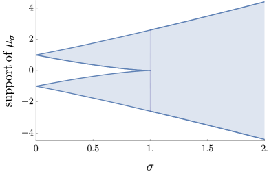
Figure 3. The support of the measure $\mu_{\sigma}=(1/2\delta_{-1}+1/2\delta_{1})\boxplus\mathrm{SC}_{\sigma}$ as a function of $\sigma$. For $\sigma<1$, the measure is supported on two intervals $\pm[L(\sigma),R(\sigma)]$, while for $\sigma\geq 1$, the support is the interval $[-R(\sigma),R(\sigma)].$

One could have obtained the result above on the support of the measure $\mu_{\sigma}$ using directly the machinery of Voiculescu’s $\mathcal{R}$-transform, see [NS06, Lecture 12]. The $\mathcal{R}$-transform of the measure $\mu_{\sigma}$ is the sum of the $\mathcal{R}$-transforms of the Bernoulli, resp. the semicircular distributions:

$$\mathcal{R}_{\mu_{\sigma}}(z)=\mathcal{R}_{\textrm{Bernoulli}}(z)+\mathcal{R}_{\textrm{SC}_{\sigma}}(z)=\frac{\sqrt{1+4z^{2}}-1}{2z}+\sigma z.$$

From the $\mathcal{R}$-transform one can obtain a cubic equation satisfied by the Cauchy transform of the measure $\mu_{\sigma}$. Then, using Stieltjes’ inversion formula, we can compute (intricate cubic roots) formulas for the density of the measure $\mu_{\sigma}$. We plot these theoretic curves against histograms of the random matrices $\mathrm{i}J_{2n}-G_{n}/\sqrt{2n}$ in Figure 4.

Figure 4. Theoretical limit densities (blue) vs. empirical eigenvalue histograms (yellow) for a single realization of $\mathrm{i}J_{2n}-G_{2n}/\sqrt{2n}$, with $n=1000$. From top to bottom, left to right: $\sigma=0.5,1,1.2,2$.

From result above, we have seen that the proper normalization of the $\mathrm{GOE}(2n,\sigma)$ matrix (with $\sigma>0$ fixed) is $(2n)^{-1/2}$, hence we need to consider elements of the ensemble $\mathrm{RQCM}(2n,\sigma/\sqrt{2n})$.

Theorem 4.1.

The limiting eigenvalue distribution of a random quantum covariance matrix $S_{2n}\in\mathrm{RQCM}(2n,\sigma/\sqrt{2n})$ is a shifted semicircular distribution $\mathrm{SC}_{R(\sigma),\sigma}$, where

$$\mathrm{d}\mathrm{SC}_{m,\sigma}=\frac{\sqrt{4\sigma^{2}-(x-m)^{2}}}{2\pi\sigma^{2}}\mathbf{1}_{|x-m|\leq 2\sigma}(x)\mathrm{d}x.$$ (4.5)

Let us record the behavior in $\sigma$ of the shift parameter $R$ from Eq. (4.2):

$$\text{as }\sigma\to 0,\qquad R(\sigma) =1+\sqrt{2}\sigma+\frac{\sigma^{2}}{4}+O(\sigma^{3})$$

$$\text{as }\sigma\to\infty,\qquad R(\sigma) =2\sigma+\frac{1}{\sigma}-\frac{5}{4\sigma^{3}}+O(\sigma^{-5}).$$

Note that the leading order of the expressions above match, respectively, the negative parts of the Bernoulli and semicircular distributions.

We now consider the partial transposition of the random covariance matrices introduced in Definition 3.2. Recall from Eq. (2.12) that a $n$-mode quantum covariance matrix $S$ satisfies the positive partial transposition (PPT) entanglement criterion with respect to the mode bipartition

$$n=m+(n-m)$$

if the following matrix is positive semidefinite:

$$S+\mathrm{i}\begin{bmatrix}J_{2m}&0_{2m\times 2(n-m)}\\ 0_{2(n-m)\times 2m}&J_{2(n-m)}\end{bmatrix}.$$

In the following proposition, we show that, in the limit of large $n$, random quantum covariance matrices satisfy automatically the PPT criterion. Later, in Section 6, we show that there exists a large proportion of PPT entangled Gaussian states.

Theorem 4.2.

Let $S_{2n}\in\mathrm{RQCM}(2n,\sigma/\sqrt{2n})$ be a normalized random quantum covariance matrix and $1\leq m=m(n)<n$ be a parameter introducing a bipartition of the modes. Then, almost surely as $n\to\infty$, the smallest eigenvalue of the matrix

$$S_{2n}+\mathrm{i}\begin{bmatrix}J_{2m}&0_{2m\times 2(n-m)}\\ 0_{2(n-m)\times 2m}&J_{2(n-m)}\end{bmatrix}$$

converges to 0. In particular, for all $\varepsilon>0$, the random quantum covariance matrix $S_{2n}+\varepsilon I_{2n}$ satisfies the PPT criterion from Eq. (2.12).

Proof.

First, note that the deterministic matrices $J_{2n}$ and $\left[\begin{smallmatrix}J_{2m}&0\\ 0&J_{2(n-m)}\end{smallmatrix}\right]$ have the same spectrum ($\pm 1$ with multiplicity $n$). Hence, the almost sure convergence of the smallest eigenvalue of the matrix from the statement follows in the same way as in the proof of Proposition 4.1. Adding an arbitrary positive number $\varepsilon$ to the random quantum covariance matrix ensures the positivity as $n\to\infty$. ∎

The purity $\mu$ of a Gaussian quantum state can be expressed in terms of its covariance matrix as [Ser17, Section 3.5], [dG19]

$$\mu=\frac{1}{\sqrt{\det S}}.$$

In the case of the model of random quantum covariance matrices we study, the asymptotic behavior of the purity can be described as follows.

Proposition 4.2.

Let $S_{2n}\in\mathrm{RQCM}(2n,\sigma/\sqrt{2n})$ be a normalized random quantum covariance matrix. Define the following quantity (see Eqs. (4.2), (4.5)):

$$\mathrm{LD}(\sigma):=\int_{R(\sigma)-2\sigma}^{R(\sigma)+2\sigma}\log(x)\mathrm{d}\mathrm{SC}_{R(\sigma),\sigma}(x).$$ (4.6)

Then, as $n\to\infty$, in probability,

$$-\frac{1}{n}\log\mu(S_{2n})\to\mathrm{LD}(\sigma).$$

In other words, the purity of a random quantum covariance matrix behaves as

$$\mu(S_{2n})\sim\exp(-n\mathrm{LD}(\sigma))$$

in the limit of large number of modes.

Proof.

The result is a consequence of the convergence of linear statistics of eigenvalues for the random matrix model in Proposition 4.1. Note that in our case, $R(\sigma)>2\sigma$, so the $\log$ function is bounded on the compact interval $[R(\sigma)-2\sigma,R(\sigma)+2\sigma)]$. ∎

The integral in Eq. (4.6) is transcendental and cannot be provided in closed form. We plot in Figure 5 the behavior of this function of $\sigma$. For $\sigma=1$, we obtain approximately

$$\mu(S_{2n})\sim\exp(-0.865668\cdot n).$$

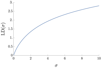
Figure 5. The rate function $\mathrm{LD}(\sigma)$ of the purity of a random quantum covariance matrix $\mu(S_{2n})\sim\exp(-n\mathrm{LD}(\sigma))$.

Let us now consider how the eigenvalue distribution of marginals of $\mathrm{RQCM}$ elements behaves in the large $n$ limit.

Proposition 4.3.

Let $S_{2n}\in\mathrm{RQCM}(2n,\sigma/\sqrt{2n})$ be a normalized random quantum covariance matrix. Consider its $m$-mode marginal $S_{2n}^{(2m)}$, where $m\to\infty$ such that $m/n\to t\in(0,1)$. Then, as $n\to\infty$, the random matrix $S_{2n}^{(2m)}$ behaves like shifted $\mathrm{RQCM}(2m,\sqrt{t}\sigma)$ element, where the asymptotic shift is given by

$$\delta_{t,\sigma}=R(\sigma)-R(\sqrt{t}\sigma).$$

In particular, its limiting eigenvalue distribution is $\mathrm{SC}_{R(\sigma),\sqrt{\sigma}}$.

Proof.

The result follows easily from Proposition 3.2:

$$S_{2n}^{(2m)}=\Big{(}\frac{G_{2n}}{\sqrt{2n}}+\lambda_{\max}(\mathrm{i}J_{2n}-G_{2n}/\sqrt{2n})\Big{)}^{(2m)}\sim\frac{G_{2m}}{\sqrt{2m}}\frac{\sqrt{2m}}{\sqrt{2n}}+R(\sigma)-R(\sqrt{t}\sigma).$$

∎

5. Symplectic eigenvalues

In this section, we compute the limiting distribution (in the large $n$ limit) of the symplectic eigenvalues of a random Gaussian covariance matrix. Recall from Section 2 that the symplectic eigenvalues of a covariance matrix $S$ are the non-negative (usual) eigenvalues of the matrix $\mathrm{i}J_{2n}\cdot S$. As in the previous section, we shall use free probability theory to compute the limiting spectrum of this matrix, in particular, the theory of $\mathcal{S}$-transform, see [NS06, Lecture 18].

We are interested in the free multiplicative product between a general semicircular distribution (with non-negative support) $\mathrm{SC}_{m,\sigma}$ and a Bernoulli distribution $\mathrm{B}:=(\delta_{-1}+\delta_{1})/2$. Recall that the (shifted) semicircular distribution with mean $m$ and variance $\sigma^{2}$ is given by

$$\mathrm{d}\mathrm{SC}_{m,\sigma}:=\frac{\sqrt{4\sigma^{2}-(x-m)^{2}}}{2\pi\sigma^{2}}\mathbf{1}_{|x-m|\leq 2\sigma}(x)\mathrm{d}x.$$

It is supported on the interval $[m-2\sigma,m+2\sigma]$; in what follows we shall assume implicitly that $m\geq 2\sigma$, although this assumption is not needed in the $\mathcal{S}$-transform computations. In free probability theory, the $\mathcal{S}$-transform has the property that, given two non-commutative random variables $x,y$, with $x\geq 0$,

$$\mathcal{S}(\sqrt{x}y\sqrt{x})=\mathcal{S}(x)\cdot\mathcal{S}(y).$$

It is a complex variable function defined by

$$\mathcal{S}(z)=\frac{1+z}{z}\chi(z),$$

where $\chi(\cdot)$ is the functional inverse of the moment generating function $\psi$

$$\psi(z)=\sum_{n=1}^{\infty}z^{n}m_{n},$$

where $m_{n}$ are the moments of the corresponding non-commutative random variable. Direct computations yield

$$\mathcal{S}_{\mathrm{B}}(z) =\frac{\sqrt{1+z}}{\sqrt{z}}$$

$$\mathcal{S}_{\mathrm{SC}_{m,\sigma}}(z) =\frac{2}{m+\sqrt{m^{2}+4\sigma^{2}z}},$$

which yield

$$\mathcal{S}_{\mathrm{B}\boxtimes\mathrm{SC}_{m,\sigma}}(z)=\frac{2\sqrt{1+z}}{\sqrt{z}(m+\sqrt{m^{2}+4\sigma^{2}z})}.$$

We now follow the inverse procedure, extracting the distribution $\mathrm{B}\boxtimes\mathrm{SC}_{m,\sigma}$ from its $\mathcal{S}$-transform. We find that the Stieltjes transform $G(z)=(1+\psi(1/z))/z$ of the free product distribution satisfies the algebraic equation

$$\frac{2\sqrt{zG-1}}{\sqrt{zG}(m+\sqrt{m^{2}+4\sigma^{2}(zG-1)})}=\frac{1}{z}.$$

After some simplifications, we find that $G$ satisfies the cubic equation

$$z\sigma^{2}G^{3}-\sigma^{2}(2z^{2}+\sigma^{2})G^{2}+z(z^{2}+2\sigma^{2}-m^{2})G-z^{2}=0.$$

We summarize these computations in the result below.

Theorem 5.1.

The limiting symplectic eigenvalue distribution of a random quantum covariance matrix $S_{2n}\in\mathrm{RQCM}(2n,\sigma/\sqrt{2n})$ is the non-negative part of the probability measure $\mathrm{B}\boxtimes\mathrm{SC}_{R(\sigma),\sigma}$, a free multiplicative convolution of a Bernoulli distribution and a non-centered semicircular distribution. The Stieltjes transform of this distribution satisfies the cubic equation

$$z\sigma^{2}G^{3}-\sigma^{2}(2z^{2}+\sigma^{2})G^{2}+z(z^{2}+2\sigma^{2}-R(\sigma)^{2})G-z^{2}=0.$$

The support of the non-negative part of this distribution is the interval $[1,\sqrt{F(\sigma)}]$, with

$$F(\sigma) :=\frac{1}{2}-\frac{\sigma^{4}}{8}+4\sigma^{2}+\sqrt{\sigma^{2}+8}\sigma+\frac{1}{8}\sqrt{\sigma^{2}+8}\sigma^{3}+$$

$$\qquad\frac{1}{64}\left(-4096\sigma^{6}+78336\sigma^{4}+49152\sigma^{2}+\right.$$

$$\qquad\left.4096\sqrt{\sigma^{2}+8}\sigma+4096\sqrt{\sigma^{2}+8}\sigma^{5}+33280\sqrt{\sigma^{2}+8}\sigma^{3}+1024\right)^{1/2}.$$

Proof.

The only statement to be proven is the formula for the right end of the support of $\mathrm{B}\boxtimes\mathrm{SC}_{R(\sigma),\sigma}$. Computing the discriminant of the cubic equation satisfied by $G$ and solving for $z$ yields a set of $6$ solutions: $z=\pm 1$, two complex solutions, and two opposite real solutions. The formula in the statement corresponds to largest positive real solution. ∎

Remark 5.1.

The behavior of the right edge of the support $\sigma\mapsto\sqrt{F(\sigma)}$ is surprisingly close to a linear function. The asymptotic behavior in the limiting cases is given by

$$\text{as $\sigma\to 0$: }\sqrt{F(\sigma)}\sim 1+2\sqrt{2}\sigma\qquad\text{ and }\qquad\text{as $\sigma\to\infty$: }\sqrt{F(\sigma)}\sim\sqrt{\frac{11}{2}+\frac{5\sqrt{5}}{2}}\sigma.$$

Writing down the cubic equation solutions is cumbersome, so we decide here to focus on some special cases and on the support of the measure $\mathrm{B}\boxtimes\mathrm{SC}_{m,\sigma}$. For example, after replacing $m=R(\sigma)$ with the value from Eq. (4.2) and taking $\sigma=1$, we find that the symplectic eigenvalues of $S_{2n}$ have, in the limit $n\to\infty$, density

$$\frac{-4x^{4}-73x^{2}+\left(-8x^{6}+510x^{4}+3\left(9\sqrt{-16x^{6}+264x^{4}-237x^{2}-11}+73\right)x^{2}+8\right)^{2/3}-4}{2\sqrt{3}\pi x\sqrt[3]{-8x^{6}+510x^{4}+3\left(9\sqrt{-16x^{6}+264x^{4}-237x^{2}-11}+73\right)x^{2}+8}}$$

supported on the interval

$$x\in\left[1,\sqrt{\frac{9\sqrt{3}}{2}+\frac{31}{4}}\right]\approx[1,3.94262].$$

We display this density along with numerical experiments in Figure 6, left panel; in the right panel we plot the analytical curve along with the histogram in the case $\sigma=10$.

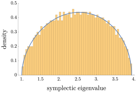
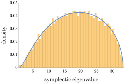
Figure 6. Numerical histograms for the symplectic eigenvalues of a random quantum covariance matrices for $n=1000$ versus theoretical densities. Left panel: $\sigma=1$; right panel: $\sigma=10$.

Concerning the physical interpretation of the above result, the largest symplectic eigenvalue $\sqrt{F(\sigma)}$ can be understood at an energy upper bound for the random quantum covariance matrix. It would be interesting to derive an explicit formula for the average energy per mode of the Gaussian state, given in the limit $n\to\infty$ as the integral

$$\int|x|\mathrm{d}(\mathrm{B}\boxtimes\mathrm{SC}_{R(\sigma),\sigma})(x).$$

Given that a tractable formula for the density of the limiting measure is unavailable in the general case, we can only compute it for special values of $\sigma$. In the case $\sigma=1$, we obtain an approximate value $2.49289$ for the energy per mode, to be compared wit the maximal energy $3.94262$ for the same value of $\sigma$.

6. Entanglement and extendability of random quantum covariance matrices

In the last part of our investigation we look at the entanglement and extendability properties of the matrices in the set $\mathrm{RQCM}(2n,\sigma)$. As was reviewed in Section 2, a Gaussian state in a bipartite state is separable if and only if its covariance matrix is completely extendable (Theorem C). The complete extendability criterion is a semi-definite program (SDP) which we can use to numerically investigate the proportions of separable and entangled Gaussian states corresponding to the random quantum covariance matrices. Since the entanglement problem is formulated as an SDP, it renders it hard to analytically analyze. It is for this reason that we resort in this section to a numerical analysis, leaving analytical results for future investigation. For comparison we also explore the PPT criterion Eq. (2.12) and numerically analyze the proportion of PPT and non-PPT random quantum covariance matrices.

Furthermore, for entangled Gaussian states we can do a finer numerical analysis to see up to which value of $k$ the corresponding random quantum covariance matrices are $k$-extendable. As pointed out in Theorem D we can take this maximum value of $k$ to depict the level of entanglement: the lower this maximum value of $k$ is the further away from complete extendability, or equivalently, from the set of separable states the covariance matrix is. Theorem D also shows that the problem of checking $k$-extendability for some fixed value of $k$ can also be cast as an SDP which allows us to perform our numerical analysis described above.

We note that in the SDPs when determining whether a random quantum covariance matrix represents a separable state or not or whether it is $k$-extendible or not we must do it within some numerical precision which we must choose. For example, we used the precision of $10^{-8}$ so that every RQCM that is within that range of being determined separable is labeled as separable. Thus, for individual samples the labels are not completely error-free but since we have used the same precision throughout our calculations, it still gives us a clear idea of the entanglement and extendibility properties of the set $\mathrm{RQCM}(2n,\sigma)$ as a whole. We also noticed that in certain cases (with very large $\sigma$ for example) the samples seem to be drawn from some kind of boundary of the set so in these cases the error caused by the numerical precision is even larger. In our calculations we tried to avoid such cases to the best of our abilities.

The numerical calculations were performed by using a Mathematica notebook containing numerical routines to sample random quantum covariance matrices and to test the extendability properties of the generated random quantum covariance matrices. The notebook is available at [LNS24].

6.1. Varying the total number of modes with even partition of subsystems

Our first analysis was done in the case when the matrices in $\mathrm{RQCM}(2n,\sigma)$ with $\sigma=1$ are assumed to correspond to bipartite states with $n=m+m$ modes for various values of $m$. In particular, we chose the cases when $n=10$, $n=20$, $n=50$ and $n=100$ in which cases we could still obtain decent sample sizes and run the extendability SDPs in reasonable time. The portions of separable/entangled states and PPT/non-PPT states are represented in Fig. 7. For the entangled states we did the finer analysis of determining for each sample what is the maximum $k$ such that the matrix is $k$-extendable and our findings can be found in Fig. 8.

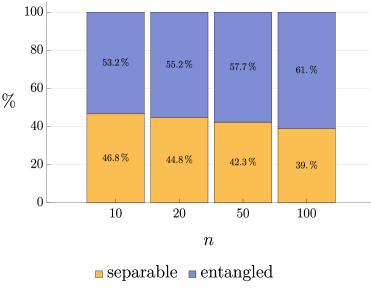
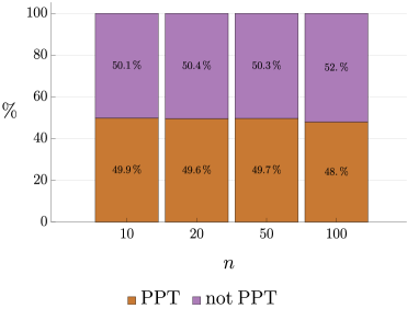
Figure 7. Numerical histograms in the case of $n=m+m$ modes for the proportion of entangled/separable states (left) and PPT/non-PPT states (right) when $\sigma=1$. The sample sizes were 50 000 for $n=10$, 10 000 for $n=20$, 5 000 for $n=50$ and $400$ for $n=100$.

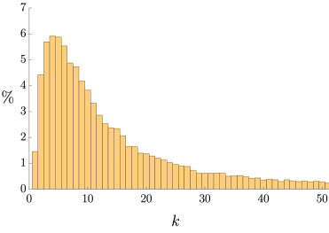
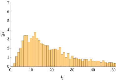
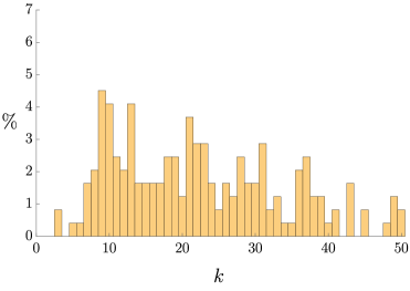
Figure 8. Numerical histograms in the case of $n=m+m$ modes ($m=5$ top left, $m=10$ top right, $m=25$ bottom left and $m=50$ bottom right) for the distribution of maximum values of $k$ for each entangled random quantum covariance matrix such that the matrix is $k$-extendable. The percentage is calculated from the total number of entangles states. The sample sizes were 50 000 for $n=10$, 10 000 for $n=20$, 5 000 for $n=50$ and $400$ for $n=100$.

From Fig. 7 it would seem that with an even partition of subsystems, the portion of separable states decreases as we increase the total number of modes. However, for all number of modes, roughly half of the samples are PPT and the proportion of PPT states vs. non-PPT states seems not to be affected by the increase of the number of modes. Further numerical analysis for the minimal eigenvalues of the PPT condition (Eq. (2.12)) for the random quantum covariance matrices shows that for all different total number of modes (with equal partitioning of subsystems) the minimal eigenvalues seem to have a Gaussian distribution around zero. However, we find that the variance of the distribution decreases as the total number of modes increases. This is supported by Theorem 4.2 which states that in the limit $n\to\infty$ the minimum eigenvalue of the PPT condition (Eq. (2.12)) for a random quantum covariance matrix converges to zero. Thus, at fixed $n$ the minimum eigenvalues have fluctuations around its average but as $n$ increases the fluctuations decrease and in the limit $n\to\infty$ the fluctuations disappear making all the states almost surely PPT.

Although a higher portion of states are entangled for increasing number of modes, from Fig. 8 we see that as the total number of modes increases, the entangled states become less entangled, i.e., they are closer to the set of separable states. However, since we are only looking at even partitions, so that as the total number of modes increases also the subsystem sizes increase, we cannot conclude from this analysis whether the increase of entangled states and the decrease in the level of entanglement results from the increase of the total number of modes or from the increase of the subsystem sizes. Thus, next we will consider the case when we fix one of the subsystem sizes and increase the total number of modes.

6.2. Varying the total number of modes with fixed subsystem size

For our subsequent analysis we chose to fix the second subsystem to consist of only two modes; for $m+1$ modes it is known that the PPT criterion Eq. (2.12) detects all the separable states.

In particular, we looked at the case when we have a total of $n=m+2$ modes for the cases when $n=10$, $n=20$, $n=50$ and $n=100$. We kept the choice $\sigma=1$ as before. The portions of separable/entangled states and PPT/non-PPT states are represented in Fig. 9. For the entangled states we did the finer analysis of determining for each sample what is the maximum $k$ such that the matrix is $k$-extendable and our findings can be found in Fig. 10.

Figure 9. Numerical histograms in the case of $n=m+2$ modes for the proportion of entangled/separable states (left) and PPT/non-PPT states (right) when $\sigma=1$ and $n\in\{10,20,50,100\}$. For all $n$ we used 5 000 samples.

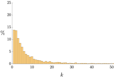
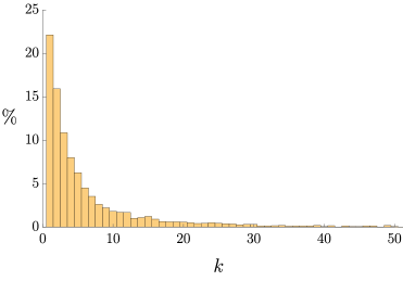
Figure 10. Numerical histograms in the case of $n=m+2$ modes ($n=10$ top left, $n=20$ top right, $n=50$ bottom left and $n=100$ bottom right) for the distribution of maximum values of $k$ for each entangled random quantum covariance matrix such that the matrix is $k$-extendable. The percentage is calculated from the total number of entangles states. For all $n$ we used 10 000 samples.

Now we see from Fig. 9 that when the second subsystem size is fixed to two modes then the number of separable states remains roughly the same even when the total number of modes is increased. This would suggest that the increase in the number of entangled states which we witnessed in Sec. 6.2 in the case of even subsystem partition is more of a result from the increase of the size of one of the subsystems rather than the increase of the total number of modes. For the proportion of PPT/non-PPT states we find a similar behaviour as in the previous case: roughly half of the samples are PPT states and even a further numerical analysis on the minimal eigenvalue distributions of the PPT condition (Eq. 2.12) for the random quantum covariance matrices again confirms this.

On the other hand, from Fig. 10 we see that when the second subsystem is fixed to have precisely two modes then the level of entanglement of the entangled states increases as the total number of modes, and thus the size of the first subsystem, increases. This is contrary to Fig. 8 in the case of even partition of subsystems which leads us to believe that the level of entanglement of the entangled random quantum covariance matrices is more proportional to the size of the first subsystem rather than the total number of modes. In order to see more evidence for this we will next fix the total number of modes and merely vary the partition of the subsystems.

6.3. Varying the partition size with fixed number of total modes

Next we looked at the case when we have a fixed number of total modes $n=m+l$, where we chose $n=20$ (for convenience), and considered the cases when the number of modes of the first subsystem are $m=2$, $m=10$ and $m=18$. Again we kept $\sigma=1$. The portions of separable/entangled states and PPT/non-PPT states are represented in Fig. 11. For the entangled states we did the finer analysis of determining for each sample what is the maximum $k$ such that the matrix is $k$-extendable and our findings can be found in Fig. 12.

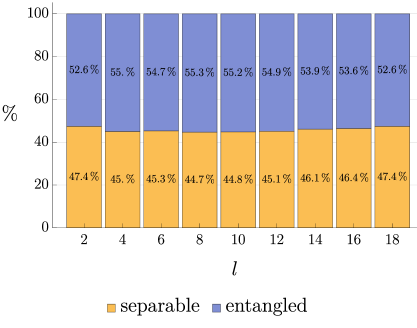
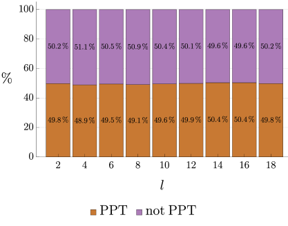
Figure 11. Numerical histograms in the case of $n=m+l=20$ modes for the proportion of entangled/separable states (left) and PPT/non-PPT states (right) when $\sigma=1$ and $l\in\{2,4,6,8,10,12,14,16,18\}$. For all subsystem partitions we used the same 10 000 samples.

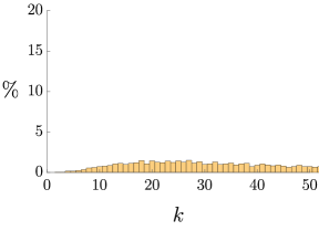
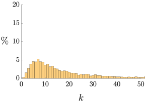
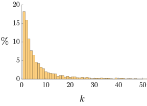
Figure 12. Numerical histograms in the case of $n=m+l=20$ modes ($m=2$ left, $m=10$ center and $m=18$ right) for the distribution of maximum values of $k$ for each entangled random quantum covariance matrix such that the matrix is $k$-extendable. The percentage is calculated from the total number of entangles states. For all subsystem partitions we used the same 10 000 samples.

By looking at Fig. 11 we find that as one of the subsystem sizes increases, then the number of separable states increases. This seems to support the claim we made earlier in Sec. 6.3: it is the increase of the size of one of the subsystems rather than the increase of the total number of modes which results in the increase of the number of the entangled states. Also Fig. 12 seems to drastically support our previous conclusion that it is the size of the first subsystem which the level of entanglement of the entangled states is proportional to. For the proportion of PPT/non-PPT states we again find a similar behaviour as in the previous cases: roughly half of the samples are PPT states and even a further numerical analysis on the minimal eigenvalue distributions of the PPT condition (Eq. 2.12) for the random quantum covariance matrices confirms this.

6.4. Varying the standard deviation $\sigma$

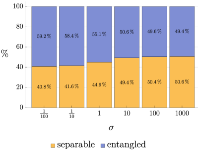
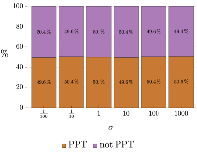
Figure 13. Numerical histograms in the case of $n=10+10$ modes for the proportion of entangled/separable states (left) and PPT/non-PPT states (right) when $\sigma\in\{\frac{1}{100},\frac{1}{10},1,10,100,1000\}$. The sample size was 10 000 for all $\sigma$.

Lastly, we want to explore how changing the parameter $\sigma$ controlling the spread of the $\mathrm{GOE}$ random matrix affects the entanglement properties of the elements in $\mathrm{RQCM}(2n,\sigma)$. In the previous cases we had fixed $\sigma=1$ but now we will vary $\sigma$ in the case when we have a fixed number of total modes $n=20$ with an even partition $n=10+10$. In particular, we look at different values of the variance parameter $\sigma\in\{\frac{1}{100},\frac{1}{10},1,10,100,1000\}$. The details of the sample sizes and the portions of separable states and PPT states is represented in Fig. 13. For the entangled states we again did the finer analysis of determining for each sample what is the maximum $k$ such that the matrix is $k$-extendible. Our findings can be found in Fig. 14.

From Fig. 13 we see that as we increase $\sigma$ also the fraction of separable states increases. This corresponds to the intuition that larger $\sigma$ yields more spread-out GOE matrices $G$ with a larger probability that $H=G$. On the other hand, models with small $\sigma$ would need to be shifted to land in the set of quantum covariance matrices. Since the resulting matrix is on the boundary of this set, the probability that it is separable tends to be smaller, see Fig. 1. In a similar vein, Fig. 14 shows that those states that are entangled will have a higher level of entanglement as $\sigma$ increases. Also it is noteworthy that as $\sigma$ increases the PPT criterion seems to be better at detecting the separable states.

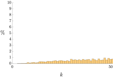
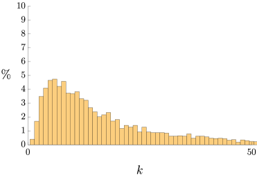
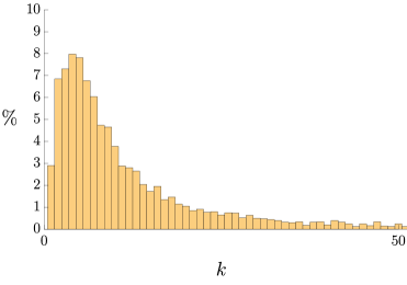
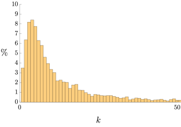
Figure 14. Numerical histograms in the case of $n=10+10$ modes ($\sigma=\frac{1}{10}$ top left, $\sigma=1$ top right, $\sigma=10$ bottom left and $\sigma=100$ bottom right) for the distribution of maximum values of $k$ for each entangled random quantum covariance matrix such that the matrix is $k$-extendable.

Acknowledgements. LL acknowledges support from the European Union’s Horizon 2020 Research and Innovation Programme under the Programme SASPRO 2 COFUND Marie Sklodowska-Curie grant agreement No. 945478 as well as from projects APVV22-0570 (DeQHOST) and VEGA 2/0183/21 (DESCOM). LL also acknowledges support from the collaboration of the French Embassy in Slovakia, the French Institute in Slovakia and the Slovak Ministry of Education, Science, Research and Sports for funding the research visit to Toulouse where this project was started. I.N. was supported by the ANR projects ESQuisses, grant number ANR-20-CE47-0014-01 and STARS, grant number ANR-20-CE40-0008, and by the PHC program Star (Applications of random matrix theory and abstract harmonic analysis to quantum information theory). R.S. acknowledges financial support from DST, Govt. of India, project number DST/ICPS/QuST/Theme- 2/2019/General Project Q-90, and the French CNRS, for supporting a visit to Toulouse, where this project was started.

References

- [ADMS95] Arvind, B. Dutta, N. Mukunda, and R. Simon. The real symplectic groups in quantum mechanics and optics. Pramana, 45:471–497, 1995.
- [AGZ10] Greg W Anderson, Alice Guionnet, and Ofer Zeitouni. An introduction to random matrices. Cambridge University Press, 2010.
- [ARL14] Gerardo Adesso, Sammy Ragy, and Antony R. Lee. Continuous variable quantum information: Gaussian states and beyond. Open Systems & Information Dynamics, 21(01n02):1440001, 2014.
- [BCY11] Fernando G. S. L. Brandão, Matthias Christandl, and Jon Yard. Faithful squashed entanglement. Comm. Math. Phys., 306(3):805–830, 2011.
- [BH13] Fernando G. S. L. Brandão and Aram W. Harrow. Quantum de Finetti theorems under local measurements with applications (extended abstract). In STOC’13—Proceedings of the 2013 ACM Symposium on Theory of Computing, pages 861–870. ACM, New York, 2013.
- [Bia97] Philippe Biane. On the free convolution with a semi-circular distribution. Indiana University Mathematics Journal, pages 705–718, 1997.
- [BPS17] B. V. Rajarama Bhat, K. R. Parthasarathy, and Ritabrata Sengupta. On the equivalence of separability and extendability of quantum states. Rev. Math. Phys., 29(4):1750012, 16, 2017.
- [Bra96] Samuel L Braunstein. Geometry of quantum inference. Physics Letters A, 219(3):169–174, 1996.
- [CDMF+11] Mireille Capitaine, Catherine Donati-Martin, Delphine Féral, Maxime Février, et al. Free convolution with a semicircular distribution and eigenvalues of spiked deformations of wigner matrices. Electron. J. Probab, 16(64):1750–1792, 2011.
- [CM14] Benoit Collins and Camille Male. The strong asymptotic freeness of Haar and deterministic matrices. Annales scientifiques de l’Ecole Normale Supérieure, 47:147–163, 2014.
- [CN16] Benoit Collins and Ion Nechita. Random matrix techniques in quantum information theory. Journal of Mathematical Physics, 57(1), 2016.
- [dG19] Maurice de Gosson. On the Purity and Entropy of Mixed Gaussian States, pages 145–158. Springer International Publishing, Cham, 2019.
- [DPS04] Andrew C. Doherty, Pablo A. Parrilo, and Federico M. Spedalieri. Complete family of separability criteria. Phys. Rev. A, 69:022308, Feb 2004.
- [FK81] Zoltán Füredi and János Komlós. The eigenvalues of random symmetric matrices. Combinatorica, 1:233–241, 1981.
- [FK19] Motohisa Fukuda and Robert König. Typical entanglement for Gaussian states. J. Math. Phys., 60(11):112203, 16, 2019.
- [GT09] Otfried Gühne and Géza Tóth. Entanglement detection. Phys. Rep., 474(1-6):1–75, 2009.
- [Hal98] Michael JW Hall. Random quantum correlations and density operator distributions. Physics Letters A, 242(3):123–129, 1998.
- [Has09] Matthew B Hastings. Superadditivity of communication capacity using entangled inputs. Nature Physics, 5(4):255–257, 2009.
- [HHHH09] Ryszard Horodecki, Paweł Horodecki, Michał Horodecki, and Karol Horodecki. Quantum entanglement. Rev. Mod. Phys., 81(2):865–942, Jun 2009.
- [HLW06] Patrick Hayden, Debbie W Leung, and Andreas Winter. Aspects of generic entanglement. Communications in Mathematical Physics, 265(1):95–117, 2006.
- [HM76] R. L. Hudson and G. R. Moody. Locally normal symmetric states and an analogue of de Finetti’s theorem. Z. Wahrscheinlichkeitstheorie und Verw. Gebiete, 33(4):343–351, 1975/76.
- [Hol11] Alexander Holevo. Probabilistic and statistical aspects of quantum theory, volume 1 of Quaderni. Monographs. Edizioni della Normale, Pisa, second edition, 2011. With a foreword from the second Russian edition by K. A. Valiev.
- [Hol12] Alexander S. Holevo. Quantum systems, channels, information, volume 16 of De Gruyter Studies in Mathematical Physics. De Gruyter, Berlin, 2012. A mathematical introduction.
- [KNP+21] Ryszard Kukulski, Ion Nechita, Ł ukasz Pawela, Zbigniew Puchał a, and Karol Życzkowski. Generating random quantum channels. J. Math. Phys., 62(6):Paper No. 062201, 24, 2021.
- [LKAW19] Ludovico Lami, Sumeet Khatri, Gerardo Adesso, and Mark M. Wilde. Extendibility of bosonic Gaussian states. Phys. Rev. Lett., 123(5):050501, 7, 2019.
- [LNS24] Leevi Leppäjärvi, Ion Nechita, and Ritabrata Sengupta. Mathematica notebook containing numerical routines used in this paper, available at https://github.com/leevi-leppajarvi/random-quantum-covariance-matrices, 2024.
- [LRW+18] Ludovico Lami, Bartosz Regula, Xin Wang, Rosanna Nichols, Andreas Winter, and Gerardo Adesso. Gaussian quantum resource theories. Phys. Rev. A, 98:022335, Aug 2018.
- [Mac63] George W. Mackey. The mathematical foundations of quantum mechanics: A lecture-note volume. W., A. Benjamin, Inc., New York-Amsterdam, 1963.
- [Mal12] Camille Male. The norm of polynomials in large random and deterministic matrices. Probability Theory and Related Fields, 154(3-4):477–532, 2012.
- [Mey93] Paul-André Meyer. Quantum probability for probabilists, volume 1538 of Lecture Notes in Mathematics. Springer-Verlag, Berlin, 1993.
- [MS17] James A Mingo and Roland Speicher. Free probability and random matrices, volume 35. Springer, 2017.
- [NC10] Michael A. Nielsen and Isaac L. Chuang. Quantum Computation and Quantum Information. Cambridge University Press, 10th anniversary edition, 2010. Cambridge Books Online.
- [NS06] Alexandru Nica and Roland Speicher. Lectures on the combinatorics of free probability, volume 13. Cambridge University Press, 2006.
- [Par92] K. R. Parthasarathy. An introduction to quantum stochastic calculus. Modern Birkhäuser Classics. Birkhäuser/Springer Basel AG, Basel, 1992. [2012 reprint of the 1992 original] [MR1164866].
- [Par05] K. R. Parthasarathy. Mathematical foundations of quantum mechanics, volume 35 of Texts and Readings in Mathematics. Hindustan Book Agency, New Delhi, 2005.
- [Par10] K. R. Parthasarathy. What is a Gaussian state? Commun. Stoch. Anal., 4(2):143–160, 2010.
- [Par13] Kalyanapuram R. Parthasarathy. The symmetry group of Gaussian states in . In Prokhorov and contemporary probability theory, volume 33 of Springer Proc. Math. Stat., pages 349–369. Springer, Heidelberg, 2013.
- [PS15a] K. R. Parthasarathy and Ritabrata Sengupta. Exchangeable, stationary and entangled chains of Gaussian states. J. Math. Phys., 56(10):102203, 11, 2015.
- [PS15b] K. R. Parthasarathy and Ritabrata Sengupta. From particle counting to Gaussian tomography. Infin. Dimens. Anal. Quantum Probab. Relat. Top., 18(4):1550023, 21, Dec 2015.
- [SDGP07] A. Serafini, O. C. O. Dahlsten, D. Gross, and M. B. Plenio. Canonical and micro-canonical typical entanglement of continuous variable systems. J. Phys. A, 40(31):9551–9576, 2007.
- [Ser17] Alessio Serafini. Quantum continuous variables. CRC Press, Boca Raton, FL, 2017. A primer of theoretical methods.
- [Sim00] R. Simon. Peres-Horodecki separability criterion for continuous variable systems. Phys. Rev. Lett., 84:2726–2729, Mar 2000.
- [Stø69] Erling Størmer. Symmetric states of infinite tensor products of -algebras. J. Functional Analysis, 3:48–68, 1969.
- [SŻ04] Hans-Jürgen Sommers and Karol Życzkowski. Statistical properties of random density matrices. Journal of Physics A: Mathematical and General, 37(35):8457, 2004.
- [VDN92] Dan V Voiculescu, Ken J Dykema, and Alexandru Nica. Free random variables. 1. American Mathematical Soc., 1992.
- [Wig55] Eugene P Wigner. Characteristic vectors of bordered matrices with infinite dimensions. Annals of Mathematics, pages 548–564, 1955.
- [WPGP+12] Christian Weedbrook, Stefano Pirandola, Raúl García-Patrón, Nicolas J. Cerf, Timothy C. Ralph, Jeffrey H. Shapiro, and Seth Lloyd. Gaussian quantum information. Rev. Mod. Phys., 84:621–669, May 2012.
- [WW01] R. F. Werner and M. M. Wolf. Bound entangled gaussian states. Phys. Rev. Lett., 86:3658–3661, Apr 2001.
- [ŻPNC11] Karol Życzkowski, Karol A Penson, Ion Nechita, and Benoit Collins. Generating random density matrices. Journal of Mathematical Physics, 52(6):062201, 2011.
- [ŻS01] Karol Życzkowski and Hans-Jürgen Sommers. Induced measures in the space of mixed quantum states. Journal of Physics A: Mathematical and General, 34(35):7111, 2001.