Numerical Approximations and Convergence Analysis of Piecewise Diffusion Markov Processes, with Application to Glioma Cell Migration

Abstract

In this paper, we focus on numerical approximations of Piecewise Diffusion Markov Processes (PDifMPs), particularly when the explicit flow maps are unavailable. Our approach is based on the thinning method for modelling the jump mechanism and combines the Euler-Maruyama scheme to approximate the underlying flow dynamics. For the proposed approximation schemes, we study both the mean-square and weak convergence. Weak convergence of the algorithms is established by a martingale problem formulation. Moreover, we employ these results to simulate the migration patterns exhibited by moving glioma cells at the microscopic level. Further, we develop and implement a splitting method for this PDifMP model and employ both the Thinned Euler-Maruyama and the splitting scheme in our simulation example, allowing us to compare both methods.

Keywords— Piecewise Diffusion Markov Processes, Thinning Method, Splitting Method,
Low Grade Glioma model

1 Introduction

Over the past decades, stochastic hybrid systems (SHS) have emerged as a powerful modelling technique in a wide range of application areas such as mathematical biology [7, 21], neuroscience [46, 14], biochemistry [52], finance [33], and power systems [39], to name a few.
A well-known and very powerful class of SHS, characterised by continuous dynamics and stochastic jumps, is the piecewise deterministic Markov process (PDMP), introduced in $1984$ by Davis [23]. Davis’s pioneering work focused on endowing PDMPs with general tools, similar to the already existing one for diffusion processes. Essentially, PDMPs form a family of non-diffusive càdlàg Markov processes, involving a deterministic motion punctuated by random jumps.
A few years later, a very general formal model for stochastic hybrid systems was proposed by Blom in [11]. This model expanded upon the foundational principles of the PDMPs by substituting the ordinary differential equations (ODEs), which govern continuous dynamics, with their stochastic counterparts. Moreover, the author introduced generalised reset maps that incorporated state-dependent distributions, characterising the probability density of the system state after each transition. This class of newly formulated hybrid systems was named Piecewise Diffusion Markov processes (PDifMPs).
Subsequently, in 2003, a follow-up work by Bujorianu et al. [16] rigorously established the theory underlying PDifMPs and defined their extended generators.
While PDifMPs are amenable to analytical solutions in certain cases, numerical approximation techniques are often required in practice. One of the main challenges in numerically approximating PDifMPs lies in handling stochastic jumps, which occur at random times and exert a substantial influence on the system dynamics. Furthermore, it is essential to efficiently combine these jumps with the discretisation of the continuous dynamics. Numerous publications have addressed numerical approximations for PDMPs, e.g. [36, 37, 49, 34, 8]. In particular, [8] provides a thorough overview of issues arising, when approximating all characteristics of PDMPs with a focus on simulating the underlying distributions. However, there appears to be a gap in the literature regarding the development and analysis of numerical schemes for PDifMPs. Although, simulations of generalised stochastic hybrid systems are presented in [12], these are limited to specific examples.
To address this issue, we propose two distinct approaches that combine different techniques for approximating both the continuous and discrete aspects of the process. Inspired by the work of Lemaire et al. [36, 37], we introduce a first approach for approximating the flow maps of PDifMPs. This approach leverages a combination of the thinning method and the Euler-Maruyama scheme. Additionally, we provide estimates for the mean-square error and introduce a framework for a weak error expansion.
Furthermore, we propose a second numerical method that integrates the thinning method with the splitting method to approximate the continuous dynamics of the process between jump times.
The fundamental idea behind the splitting method is to decompose the stochastic differential equations (SDEs) governing the continuous component of the process into exactly solvable subequations, derive their solutions and compose them in a suitable way. We refer to [41, 18] for a thorough discussion of splitting methods for ODEs and to [15, 1, 3, 50, 47] among many others, for references considering extensions to SDEs. To the best of our knowledge, this approach has not yet been explored in the context of PDifMPs.

As an application we consider a PDifMP describing glioma cell migration at a microscopic scale, simplifying the model to one dimension for clarity of exposition. Gliomas, the most prevalent type of intracranial tumour, account for over $70\%$ of all brain cancers. These tumours arise from mutated glial cells, which are a type of cell that provides physical and chemical support to neurons [43]. For an extensive discussion on low-grade gliomas and various mathematical models for studying brain tumours we refer to our work [42] and the references therein.
The paper is organised as follows. In Section 2, we provide a concise introduction to PDifMPs. Section 3 introduces the Thinned Euler-Maruyama (TEM) method for PDifMPs. Sections 4 and 5 are dedicated to the numerical analysis, exploring both mean-square and weak convergence. Section 6 presents an extended model from [42], considering microenvironmental effects on cellular movement, and includes numerical simulations using the TEM method, comparing it with the splitting method. These simulations focus on the impact of parameters like the jump intensity of PDifMPs and the time step size. Section 7 concludes with a review of our findings and discusses potential future research directions.

2 Preliminaries

In this section, we present the preliminary concepts necessary to understand PDifMPs. For more detailed information, we refer the reader to [17, 16, 6].
We consider a complete probability space $\left(\Omega,\mathcal{F},(\mathcal{F})_{t\geq 0},\mathbb{P}\right)$ with filtration $(\mathcal{F})_{t\geq 0}$ on $\Omega$ satisfying the usual conditions, i.e $(\mathcal{F})_{t\geq 0}$ is right continuous and $\mathcal{F}_{0}$ contains all $\mathbb{P}$-null sets in $\mathcal{F}$. Further, we consider $(W_{t})_{t\in[0,T]}\in\mathbb{R}^{m}$, $m\in\mathbb{N}$ and $T>0$, to be a standard Wiener process defined on $\left(\Omega,\mathcal{F},(\mathcal{F})_{t\geq 0},\mathbb{P}\right)$. We assume that $W_{t}$ is $\mathcal{F}_{t}$-adapted.
The PDifMP we consider consists of two non-exploding processes $(y_{t},v_{t})$, with values in $E=E_{1}\times\mathbf{V}$. Here, $E_{1}$ and $\mathbf{V}$ are subsets of $\mathbb{R}^{d}$, $d\in\mathbb{N}$, such that $\mathbf{V}$ is finite or a countable set. The Borel $\sigma$-algebra $\mathcal{B}(E)$ is generated by the topology of $E$.
The first stochastic component $(y_{t})_{t\in[0,T]}$ possesses continuous paths in $E_{1}$, while the second component $(v_{t})_{t\in[0,T]}$ is a jump process with right-continuous paths and piecewise constant values in $\mathbf{V}$. Additionally, we denote by $(T_{n})_{n\in\mathbb{N}}$ the times at which the second component jumps. These times form a sequence of randomly distributed grid points in the interval $[0,T]$.
The dynamics of the PDifMP $(x_{t})=(y_{t},v_{t})$, $t\in[0,T]$, on $(E,\mathcal{B}(E))$ are defined by its characteristic triple $(\phi,\lambda,\mathcal{Q})$. The parameter $\phi:[0,T]\times E\rightarrow E_{1}$, given by $(t,x)\mapsto\phi(t,x)$, represents the stochastic flow map of the continuous component $(y_{t})_{t\in[0,T]}$. Starting at $T_{0}=0$ with an initial value $x_{0}=(y_{0},v_{0})\in E$, the process $\phi(t,x)$ represents the solution of a sequence of SDEs over consecutive intervals $[T_{n},T_{n+1})$ with random lengths. At each random point $T_{n}\in[0,T]$, $n\geq 1$, there are updated initial values $x_{n}=(y_{n},v_{n})\in E$. Here, $y_{n}$ serves as the initial value, and $v_{n}$ acts as a parameter in SDE (1), stated below, defined on the interval $[T_{n},T_{n+1})$.
For $p\geq 1$, let $\mathcal{L}_{\text{ad}}\left(\Omega,L^{p}[T_{n},T_{n+1}]\right)$ denote the class of random processes that are $\mathcal{F}_{t}$-adapted and exhibit almost surely $p$-integrable sample paths. In the context of Equation (1), we define the drift vector $b(\cdot,v_{n})$ mapping $E$ into $\mathbb{R}^{d}$ as an element of $\mathcal{L}_{\text{ad}}\left(\Omega,L^{1}[T_{n},T_{n+1}]\right)$. Further, the diffusion matrix $\sigma(\cdot,v_{n})$, mapping $E$ into $\mathbb{R}^{{d}\times m}$ is a class $\mathcal{L}_{ad}\left(\Omega,L^{2}[T_{n},T_{n+1}]\right)$ function. Let

$$\left\{\begin{array}[]{ll}d\phi(t,x_{n})=b(\phi(t,x_{n}),v_{n})dt+\sigma(\phi(t,x_{n}),v_{n})dW_{t},\qquad t\in[T_{n},T_{n+1}),\\[5.69046pt] \phi(T_{n},x_{n})=y_{n}.\end{array}\right.$$ (1)

At the end point $T_{n+1}$ of each interval, $y_{n+1}$ is set to the current value of $\phi(\,\cdot\,,x_{n})$ to ensure the continuity of the path. Further, a new value $v_{n+1}$ is chosen as fixed parameter for the next interval according to the jump mechanism described below. Equation (1) can be formulated equivalently as

$$\phi(t,x_{n})=y_{n}+\int_{0}^{t}b(\phi(s,x_{n}),v_{n})ds+\int_{0}^{t}\sigma(\phi(s,x_{n}),v_{n})dW_{s},\qquad t\in[T_{n},T_{n+1}).$$ (2)

For ease of understanding, we adopt the notation $x_{t}=(y_{t},v_{t})$ to represent the sample paths of the PDifMP, with $x=(y,v)$ denoting the initial conditions following each jump. Henceforth, unless otherwise specified, $x=(y,v)$ consistently indicates the starting point for each interval, irrespective of the specific time point under consideration.
The following theorem establishes the existence of a unique solution for Equation (2) in $E$.

Theorem 2.1 (Mao [40]).

Assume that there exist two positive constants $K_{1}$ and $K_{2}$, such that

1. (Lipschitz condition) for all $x=(y,v)\in E$, $\tilde{x}=(\tilde{y},v)\in E$ and $\phi:[0,T]\times E\rightarrow E_{1}$

   $$\lvert b(\phi(t,x),v)-b(\phi(t,\tilde{x}),v)\rvert^{2}\bigvee\lvert\sigma(\phi(t,x),v)-\sigma(\phi(t,\tilde{x}),v)\rvert^{2}\leq K_{1}\lvert\phi(t,x)-\phi(t,\tilde{x})\rvert^{2},$$ (3)

2. (Linear growth condition) for all $(t,x)\in[0,T]\times E$

   $$\lvert b(\phi(t,x),v)\rvert^{2}\bigvee\lvert\sigma(\phi(t,x),v)\rvert^{2}\leq K_{2}(1+|\phi(x)|^{2}).$$ (4)

Then, for any $v\in\mathbf{V}$, there exists a unique solution to Equation (2) in $E$.

The stochastic flow $\phi$ possesses the semi-group property

$$\phi\big{(}(t+s),(\,\cdot\,,v)\big{)}=\phi\big{(}t,\,(\phi(s,(\,\cdot\,,v)),v)\big{)}\,,\quad\forall\,t,\,s\in[0,T].$$ (5)

The jump mechanism of the PDifMP is governed by the remaining components of its characteristic triple, namely $\lambda$ and $\mathcal{Q}$. Specifically, the function ${\lambda:E\rightarrow\mathbb{R}_{+}}$ quantifies the rate at which jumps take place in the second component of the process $(x_{t})_{t\in[0,T]}$, which in turn determines the sequence of random times $(T_{n})_{n>0}$.

Assumption 2.1.

Let $\lambda:E\rightarrow\mathbb{R}_{+}$ be a measurable function. For all $\omega\in\Omega$, $x=(y,v)\in E$, and $T>0$, we assume that

$$\int_{0}^{T}\lambda(\phi(t,x),v)dt<\infty\hskip 28.45274pt\text{and}\hskip 28.45274pt\int_{0}^{\infty}\lambda(\phi(t,x),v)dt=\infty.$$ (6)

The first condition in Assumption 2.1 ensures that the total jump rate over any finite time interval is bounded, preventing excessively frequent jumps. The second condition ensures that the total jump rate over infinite time intervals is unbounded, allowing for a nontrivial occurrence of jumps over time.
Additionally, the transition kernel $\mathcal{Q}:(E,\mathcal{B}(E))\rightarrow[0,1]$ determines the new value of the second component following a jump event. It defines the probability distribution that governs the transition from the pre-jump state to the post-jump state. Importantly, the condition $\mathcal{Q}(x,{x})=0$ holds for all $x\in E$, effectively preventing the process from having a no-move jump.

Assumption 2.2.

For all $x\in\overline{E}$, where $\overline{E}$ denotes the closure of the set $E$, the function $\mathcal{Q}(x,\,\cdot\,)$ is a probability measure. Further, For all $A\in\mathcal{B}(E)$, $\mathcal{Q}(\,\cdot\,,A)$ is measurable.

In this work, we only consider PDifMPs with a continuous state component $y$. This implies that for any $A\in\mathcal{B}(E_{1})$ and $B\in\mathcal{B}(\mathbf{V})$, the following holds

$$\mathcal{Q}(x,A\times B)=\mathcal{Q}(x,A)\delta_{y}(B),$$ (7)

where $\delta$ refers to the Dirac delta function.

Definition 2.1.

For any $t\in[T_{n},T]$ with $n\geq 0$, the survival function of the inter-jump times $\mathcal{S}(t,x)$ is defined as follows

$$\mathcal{S}(t,x):=\exp\left(-\int_{T_{n}}^{t}\lambda(\phi(s,x),v)ds\right),\qquad x\in E.$$ (8)

The function $\mathcal{S}(t,x)$ represents the probability of no jump occurring in the time interval $[T_{n},t)$ given that the process is in the initial state $x$. For simplicity, we assume that $\mathcal{S}$ is explicitly invertible, and refer to several works where an approximation of the inverse is proposed [49, 55, 36].
Further, we introduce the uniformly distributed random variable $\mathcal{U}$ on $[0,1]$ and define the generalised inverse of $\mathcal{S}(t,x)$ as $\zeta:[0,1]\times E\rightarrow\mathbb{R}_{+}$, given by

$$\zeta(\mathcal{U},x)=\inf\{t\in[0,T]\,;\,\mathcal{S}(t,x)\leq\mathcal{U}\}.$$ (9)

Here, $\zeta(\mathcal{U},x)$ serves as a threshold time that determines the occurrence of jumps in the process and their associated probabilities.

Definition 2.2.

Let $\psi:[0,1]\times E\rightarrow E$ be a measurable function. We say that $\psi$ is the generalised inverse function of $\mathcal{Q}$ if, for any initial state $x\in E$ and any measurable set $A\in\mathcal{B}(E)$, the following holds

$$\mathbb{P}(\psi(\mathcal{U},x)\in A)=\mathcal{Q}(x,A).$$ (10)

For each $\omega\in\Omega$, the random variable $\psi(\mathcal{U}(\omega),x(\omega))$ describes the post-jump locations of the second component of $x$.
For ease of exposition we only discuss the case $d=1$ throughout the rest of the article, the results also hold for $d>1$.

3 Thinned Euler-Maruyama Method for PDifMP

In this section, we build upon the work in [37] by adapting the PDMP simulation techniques for PDifMPs. To do that, we propose a simulation technique that we call the thinned Euler-Maruyama method (TEM). This method offers a twofold approach to approximating PDifMPs. Firstly, it addresses scenarios where the flow maps within PDifMPs may not have explicit analytical solutions. Here, we employ the Euler-Maruyama method to approximate the flow maps between jump events. Secondly, we leverage the thinning method to approximate the jump times within the PDifMP.
The thinning method, initially developed for Non-Homogeneous Poisson Processes (NHPPs) [38], and later adapted to the simulation of the jump rate of PDMPs, is akin to an acceptance-rejection algorithm, [10, 36, 37]. It effectively simulates PDifMP jump times by generating potential transition times from a homogeneous Poisson process with rate $\lambda^{*}$, $\lambda^{*}>0$. These times are accepted with a probability determined by the ratio $\lambda(\,\cdot\,)/\lambda^{*}$.
Note that our approach assumes a globally bounded jump rate $\lambda^{*}$ as an upper bound. However, the use of Poisson thinning can be extended to varying bounds $\lambda^{*}(t)$ along trajectories. This extension is feasible as long as it remains possible to simulate from a NHPP with rate $\lambda^{*}(t)$. We refer to [13, 9, 36] and the references therein for more details about Poisson thinning.

3.1 Simulation of PDifMPs and thinning

Let $T>0$ be a fixed time horizon. Let $(N^{*}_{t})_{t\in[0,T]}$ be a homogeneous Poisson process on the probability space $(\Omega,\mathcal{F},\mathbb{P})$ with intensity $\lambda^{*}$. We assume that $\lambda^{*}$ satisfies the following assumption :

Assumption 3.1.

There exists a finite positive constant $\lambda^{*}$ such that, for all $x\in E$, ${\lambda(x)\leq\lambda^{*}}$.

Let $(T^{*}_{k})_{k\geq 1}$ denote the successive jump times of $(N^{*}_{t})_{t\in[0,T]}$ with $T^{*}_{0}=0$. Additionally, we define two i.i.d sequences of random variables; $(\mathcal{U}_{k})_{k\geq 1}$ and $(\mathcal{V}_{k})_{k\geq 1}$, both uniformly distributed on the interval $[0,1]$. These sequences are independent of each other and independent of $(T^{*}_{k})_{k\geq 1}$.
Let $(x_{t})_{t\in[0,T]}$ be a PDifMP satisfying (7). Using these sequences, we iteratively construct a sequence of jump times $(T_{n})_{n\geq 0}$ and post-jump locations $(y_{n},v_{n})_{n\geq 0}$ of $(x_{t})_{t\in[0,T]}$ as follows.
Starting at $T_{0}$ with a fixed initial state $(y_{0},v_{0})\in E$, we determine the subsequent jump time $T_{1}$ of the process $(x_{t})_{t\in[0,T]}$ using the thinning technique applied to the sequence $(T^{*}_{k})_{k\geq 1}$:

$$T_{1}:=T^{*}_{\tau_{1}},$$ (11)

where $\tau_{1}$ is given by

$$\tau_{1}:=\inf\left\{k>0:\mathcal{U}_{k}\lambda^{*}\leq\lambda\big{(}\phi(T^{*}_{k},x_{0}),v_{0}\big{)}\right\}.$$ (12)

Since $\mathbf{V}$ is at most a countable set, we can write it as $\mathbf{V}=\{k_{1},\ldots,k_{|\mathbf{V}|}\}$, where $|\mathbf{V}|$ is the cardinal number of the set $\mathbf{V}$. This implies that we can provide a more specific form of the generalised inverse function of $\mathcal{Q}$ given in Definition 2.2. To this end, we introduce the following definition.

Definition 3.1.

For $j\in\{1,\ldots,|\mathbf{V}|\}$, let $a_{j}$ define the cumulative distribution function of $\mathcal{Q}$ such that, for any $x=(y,v)\in E$, and $\tilde{y}\in E_{1}$, we have $a_{0}(x)=0$ and

$$a_{j}(x)=a_{j}(y,v):=\sum_{i=1}^{j}\mathcal{Q}\big{(}(y,v),\{\tilde{y},k_{i}\}\big{)}.$$ (13)

Then, for any generic $x\in E$, the discretised form of the inverse of the cumulative distribution function $\psi(\,\cdot\,,x)$ of $\mathcal{Q}(x,\,\cdot\,)$ is given by

$$\psi(u,x):=\sum_{i=1}^{|\mathbf{V}|}k_{i}\mathbbm{1}_{a_{i-1}(x)<u\leq a_{i}(x)},\quad\forall\,x\in E,\,\forall\,u\in[0,1].$$ (14)

Now, we can construct $(y_{1},v_{1})$ from the uniform random variable $\mathcal{V}_{1}$ and the function $\psi$ defined in (14) as

$$(y_{1},v_{1})= \big{(}\phi(T^{*}_{\tau_{1}},x_{0}),\psi(\mathcal{V}_{1},(\phi(T^{*}_{\tau_{1}},x_{0}),v_{0}))\big{)},$$

$$= \big{(}\phi(T_{1},x_{0}),\psi(\mathcal{V}_{1},(\phi(T_{1},x_{0}),v_{0}))\big{)}.$$

Conditioning on $(\tau_{1},(T^{*}_{k})_{k\leq\tau_{1}})$, the distribution of $(y_{1},v_{1})$ is determined by the transition kernel $\mathcal{Q}$ evaluated at the state $(\phi(T^{*}_{\tau_{1}},x_{0}),v_{0})$. In other words, using (7), the conditional distribution of $(y_{1},v_{1})$ is given by

$$\sum_{k\in\mathbf{V}}\mathcal{Q}\big{(}(\phi(T^{*}_{\tau_{1}},x_{0}),v_{0}),\{k\}\big{)}\delta_{(k,\phi_{(T^{*}_{\tau_{1}},x_{0})})}.$$

Let $(\tau_{n-1},(T^{*}_{k})_{k\leq\tau_{n-1}},(y_{n-1},v_{n-1}))$, $n>1$, be the information obtained up to time $T_{n-1}$. To construct $T_{n}$, we perform thinning on the point process $(T^{*}_{k})$ based on the process being in the state $(y_{n-1},v_{n-1})$ and time $\tau_{n-1}$ for $k\leq\tau_{n-1}$. This is done by removing points $T^{*}_{k}$ for which the corresponding random variable $\mathcal{U}_{k}$ is greater than $\lambda\big{(}\phi(T^{*}_{k}-T^{*}_{\tau_{n-1}},x_{n-1}),v_{n-1}\big{)}/\lambda^{*}$. The resulting thinned point process is denoted by

$$T_{n}:=T^{*}_{\tau_{n}},$$ (15)

where

$$\tau_{n}:=\inf\{k>\tau_{n-1}\,:\,\mathcal{U}_{k}\lambda^{*}\leq\lambda\big{(}\phi(T^{*}_{k}-T^{*}_{\tau_{n-1}},x_{n-1}),v_{n-1}\big{)}\}.$$ (16)

This process repeats for each jump event $n$, and the resulting PDifMP $(y_{n},v_{n})$ evolves in accordance with the defined jump times and post-jump states such that

$$(y_{n},v_{n})= \big{(}\phi(T^{*}_{\tau_{n}}-T^{*}_{\tau_{n-1}},x_{n-1}),\psi(\mathcal{V}_{n},(\phi(T^{*}_{\tau_{n}}-T^{*}_{\tau_{n-1}},x_{n-1}),v_{n-1}))\big{)},$$

$$= \big{(}\phi(T_{\tau_{n}}-T_{\tau_{n-1}},x_{n-1}),\psi(\mathcal{V}_{n},(\phi(T_{\tau_{n}}-T_{\tau_{n-1}},x_{n-1}),v_{n-1}))\big{)}.$$

Next, we define the PDifMP $(x_{t})_{t\in[0,T]}$ at time $T_{n}$ from the sequence $(y_{n},v_{n})$ by

$$x_{t}:=\big{(}\phi((t-T_{n}),x_{n}),v_{n}\big{)},\quad t\in[T_{n},T_{n+1}).$$ (17)

Therefore, for $n\geq 1$, $x_{T_{n}}=(y_{n},v_{n})$ and the pre-jump state $x^{-}_{T_{n}}=(y_{n},v_{n-1})$.
Furthermore, we define the counting process $N_{t}$ associated with the jump times $T_{n}$ as

$$N_{t}:=\sum_{n\geq 1}\mathbbm{1}_{T_{n}\leq t}.$$ (18)

We require that the counting process $N_{t}$ satisfies the following assumption for every state $x\in E$ and $t\in[0,T]$.

Assumption 3.2.

The expected value of $N_{t}$ is finite, i.e., $\mathbb{E}[N_{t}]<\infty$.

3.2 Approximation of the flow maps

In practical applications, it is often difficult to obtain explicit expressions for the characteristics of PDifMPs when certain conditions are not met. For an extensive review and detailed discussion on various simulation methods applicable to these characteristics, we refer the reader to [8].
In this article, we propose two approximation schemes for the function $\phi$; the Euler-Maruyama scheme for general applications, and the splitting method for a particular model (see Section 6). We combine both methods with the thinning technique for the jump times and analyse this combination with the Euler-Maruyama method (see Sections 4-5).
Throughout our analysis, we assume that $b$ and $\sigma$ satisfy the assumptions stated in Theorem 2.1 for all $v\in\mathbf{V}$. For any $x=(y,v)\in E$, we denote by $\phi(t,x)$, $t\in[0,T]$, the unique solution of the SDE

$$\left\{\begin{array}[]{ll}d\phi(t,x_{t})&=b(\phi(t,y_{t}),v_{t})dt+\sigma(\phi(t,y_{t}),v_{t})dW_{t},\\ \phi(0,x)&=y,\end{array}\right.$$ (19)

where $y$ can be a constant or an $\mathcal{F}_{0}$-measurable random variable. Note that, the $0$ in $\phi(0,x)$ is a symbolic reset point, which updates $y$ to the system state at the beginning of each jump, thereby dynamically setting the initial condition for the evolution of $\phi$.
Now, given a time step $h>0$, we define the partition points of the interval $[0,T]$ as $\overline{t}_{i}=ih$ for $i\geq 0$. For all $x=(y,v)\in E$, we iteratively construct the discrete-time process $\overline{y}_{i}$ as follows:

$$\overline{y}_{i+1}=\overline{y}_{i}+b(\overline{t}_{i},(\overline{y}_{i},v))h+\sigma(\overline{t}_{i},(\overline{x}_{i},v))\Delta W_{i},$$ (20)

where $\Delta W_{i}=W_{\overline{t}_{i+1}}-W_{\overline{t}_{i}}$ is the increment of a standard Wiener process between times $\overline{t}_{i}$ and $\overline{t}_{i+1}$.
For any $x=(y,v)\in E$ and $t\in[\overline{t}_{i},\overline{t}_{i+1}]$, we set the continuous time interpolation of the numerical solution

$$\overline{\phi}(t,x)=\overline{y}_{i}+b(\overline{t}_{i},\overline{x}_{i})(t-\overline{t}_{i})+\sigma(\overline{t}_{i},\overline{x}_{i})(W_{t}-W_{\overline{t}_{i}}).$$ (21)

In other words, the scheme approximates the coefficients $b$ and $\sigma$ as piecewise constant within each time interval $t\in[\overline{t}_{i},\overline{t}_{i+1}]$. Note that $\overline{y}_{i}$ in Equation (21) represents the starting value for each successive time interval $[t_{i},t_{i+1}]$, rather than the post-jump values.
To ensure that the flow maps and their approximations remain bounded in expectation for all $v\in\mathbf{V}$, we introduce the following lemma.

Lemma 3.1.

(Mao [40]) Assuming the linear growth condition (4) holds for all $x=(y,v)\in E$ with $y=\overline{y}$, there exists a positive constant $K$ such that the functions $\phi(t,x)$ and $\overline{\phi}$ satisfy

$$\mathbb{E}[\sup_{t\in[0,T]}\lvert\phi(t,x)\rvert^{2}]\leq(1+3\mathbb{E}\lvert y\rvert^{2})e^{3KT(T+1)},$$

and

$$\mathbb{E}[\sup_{t\in[0,T]}\lvert\overline{\phi}(t,x)\rvert^{2}]\leq(1+3\mathbb{E}\lvert y\rvert^{2})e^{3KT(T+1)}.$$

The purpose of this construction is to approximate the solution of the PDifMP $(x_{t})_{t\in[0,T]}$ by a process $(\overline{x}_{t})_{t\in[0,T]}$. The approach involves simulating the continuous part of $(x_{t})_{t\in[0,T]}$ using the Euler-Maruyama scheme with a step size $h$ and determining the jump times by simulating a Poisson process with intensity function $\lambda(\overline{\phi}(t,x))$. The construction follows these steps:

1. At time $t=0$, the continuous stochastic component $y_{t}$ of $(x_{t})_{t\in[0,T]}$ is initialised at $y_{0}=y$. Then, the Euler-Maruyama scheme is used to construct a discrete-time process $\overline{y}_{i}$, and define the piecewise linear interpolation $\overline{\phi}(t,x)$ as in Equation (21).

2. The continuous stochastic component $y_{t}$ follows the flow $\overline{\phi}(t,x_{0})$ until the next jump time $\overline{T}_{1}$ occurs, which is constructed as in Equations (11) and (12), where we replace $\phi(T^{*}_{k},x_{0})$ by $\overline{\phi}(T^{*}_{k},x_{0})$.

3. At time $\overline{T}_{1}$, the continuous component of $\overline{x}_{\overline{T}_{1}}$ is set to $\overline{\phi}(\overline{T}_{1},x_{0}):=\overline{y}_{1}$ since the continuous state does not undergo any jumps until $\overline{T}_{1}$.

4. Then, when $\overline{v}_{0}$ jumps to $\overline{v}_{1}$, the procedure is iterated with the new flow $\overline{\phi}(t-\overline{T}_{1},\overline{x}_{1})$ until the next jump time $\overline{T}_{2}$ with flow $\overline{\phi}(T^{*}_{k}-\overline{T}_{1},\overline{x}_{1})$.

The recursive construction of the process $(\overline{x}_{t})_{t\in[0,T]}$ continues until the final time $T$ is reached, providing an approximation of the PDifMP $(x_{t})_{t\in[0,T]}$. Note that, while both processes are derived from the same data $N^{*}_{t}$, $\mathcal{U}_{k}$ and $\mathcal{V}_{k}$, there’s a probability that they may jump at different times and to different states. However, considering certain types of PDifMPs where the jump characteristics $(\lambda,\mathcal{Q})$ depend only on the jump component $v$, this PDifMP and its approximation always jump at the same times, and their $v$-components jump to exactly the same states. These concepts are further elaborated in [24], primarily focusing on PDMPs, but their extension to PDifMPs is straightforward.

Remark 3.1.

Due to the dependence of the intensity function on the entire path of the continuous state, the flow of the Euler-Maruyama scheme needs to be employed at each step to determine the intensity function at the current time.

Notation 3.1.

Hereafter, we denote by $\overline{T}_{n}$ the sequence of jump times of the process $(\overline{x}_{t})_{t\in[0,T]}$ and by $(\overline{N}_{t})_{t\in[0,T]}$ the associated counting process.

Remark 3.2.

(Adaptive Grid) Our approach, in contrast to traditional Euler-Maruyama methods with fixed time grids, employs a jump-adapted time discretisation scheme as in [48]. This method dynamically adjusts the discretisation grid to match the process dynamics. The time points of interest $\overline{T}_{n},\{n=0,\ldots,\overline{N}_{T}\}$ are determined by (15) and (16), where $\overline{N}_{T}$ is the total number of intervals in the adaptive grid. For each interval $[\overline{T}_{n},\overline{T}_{n+1})$, we introduce grid points

$$\{\overline{T}_{n}+kh\},\quad k=0,\ldots,\left(\frac{(\overline{T}_{n+1}\wedge T)-\overline{T}_{n}}{h}\right),$$

to ensure an adaptive number of subdivisions based on the process variability and the rate of change.

For later purposes, we introduce the following results.

Definition 3.2.

Analogously to [37], we define $\overline{\tau}^{\star}:=\inf\{k>0:(\tau_{k},v_{k})\neq(\overline{\tau}_{k},\overline{v}_{k})\}$.

The random variable $\overline{\tau}^{\star}$ allows us to partition the trajectories of the couple of processes $(x_{t},\overline{x}_{t})$ based on whether the first thinned point in the approximating process occurs at the same time as in the true process. More specifically, we can define the following event:

$$\{\min(T_{\overline{\tau}^{\star}},\overline{T}_{\overline{\tau}^{\star}})>T\}=\{N_{T}=\overline{N}_{T},\,(T_{1},v_{1})=(\overline{T}_{1},\overline{v}_{1}),\ldots,(T_{N_{T}},v_{N_{T}})=(\overline{T}_{\overline{N}_{T}},\overline{v}_{\overline{N}_{T}})\}.$$ (22)

Theorem 3.1.

(Yuan et al. [58]) Assuming the global Lipschitz conditions (3) in Theorem 2.1, we have

$$\mathbb{E}[\sup_{t\in[0,T]}|\phi(t,x)-\overline{\phi}(t,x)|^{2}]\leq C_{2}h,\quad\forall x\in E,$$ (23)

where $C_{2}$ is a positive constant independent of $v$ and $h$.

Lemma 3.2.

Assume that the assumptions of Theorem 2.1 are verified. Then, for all $(y_{1},v)\in E$ and $(y_{2},v)\in E$, there exists a positive constant $C_{2}$ independent of $v$ and $h$ such that

$$\mathbb{E}[\sup_{t\in[0,T]}|\phi(t,(y_{1},v))-\phi(t,(y_{2},v))|^{2}]\leq e^{C_{1}T}|y_{1}-y_{2}|^{2},$$ (24)

where $y_{1}$ and $y_{2}$ refer to the initial conditions, and they are updated after each jump.

Proof.

We refer to Appendix A for the proof of Lemma 3.2. ∎

Following the idea in [37], we introduce the following lemmas, to provide a quantitative estimate for the difference between the exact solution $\phi$ and the numerical solution $\overline{\phi}$ in terms of the initial conditions and the time step size.

Lemma 3.3.

Assume that the conditions of Theorem 2.1 hold. Let $\phi(t,x)=\phi(t,(y_{1},v))$ and $\overline{\phi}(t,x)=\overline{\phi}(t,(y_{2},v))$ be the exact and approximating solutions, respectively, of the system (19) with deterministic initial conditions $(y_{1},y_{2})\in E_{1}^{2}$.

1. For all fixed $\omega\in\Omega$, there exist two positive constants $C_{1}$ and $C_{2}$ independent of $v$ and $h$ such that the following holds

   $$\sup_{t\in[0,T]}|\phi(t,x)-\overline{\phi}(t,x)|\leq e^{C_{1}T}|y_{1}-y_{2}|+C_{2}h,\quad\forall v\in\mathbf{V},\,\,\forall\,(y_{1},y_{2})\in E_{1}^{2}.$$ (25)

2. For all fixed $t\in[0,T]$, there exist two positive constants $C_{3}$ and $C_{4}$ independent of $v$ and $h$ such that the following holds

   $$\mathbb{E}[\sup_{t\in[0,T]}|\phi(t,x)-\overline{\phi}(t,x)|^{2}]\leq e^{C_{3}T}|y_{1}-y_{2}|^{2}+C_{4}h,\quad\forall\,v\in\mathbf{V},\,\,\forall\,(y_{1},y_{2})\in E_{1}^{2}.$$ (26)

Proof.

The proof is straightforward using Theorem 3.1 and Lemma 3.2. ∎

Lemma 3.4.

Let $\phi$ and $\overline{\phi}$ satisfy the conditions of Lemma 3.3. Let $(t_{n})_{n\geq 0}$ be an increasing sequence of non-negative real numbers with $t_{0}=0$ and let $(\alpha_{n})_{n\geq 0}$ be a sequence of $\mathbf{V}$-valued components. For a given $y\in E_{1}$, we define iteratively the sequences $(\beta_{n})_{n\geq 0}$ and $(\overline{\beta}_{n})_{n\geq 0}$ as follows

$$\left\{\begin{array}[]{ll}\beta_{n}&=\phi((t_{n}-t_{n-1}),(\beta_{n-1},\alpha_{n-1})),\\ \beta_{0}&=y,\end{array}\right.$$

and

$$\left\{\begin{array}[]{ll}\overline{\beta}_{n}&=\overline{\phi}((t_{n}-t_{n-1}),(\overline{\beta}_{n-1},\alpha_{n-1})),\\ \overline{\beta}_{0}&=y.\end{array}\right.$$

1. For all fixed $\omega\in\Omega$, for all $n\geq 1$ and for all $C_{5}>0$ and $C_{6}>0$, we have

   $$|\overline{\beta}_{n}-\beta_{n}|\leq e^{C_{5}t_{n}}nC_{6}h,$$ (27)

   where $C_{5}$ and $C_{6}$ are independent of the discretisation step size $h$.

2. For all fixed $t\in[0,T]$, for all $n\geq 1$ and for all $C_{7}>0$ and $C_{8}>0$, we have

   $$\mathbb{E}[|\overline{\beta}_{n}-\beta_{n}|]^{2}\leq e^{C_{7}t_{n}}nC_{8}h,$$ (28)

   where $C_{7}$ and $C_{8}$ are independent of the discretisation step size $h$.

Proof.

We present here the proof of the second part of Lemma 3.4, where $\eqref{Beta_est_fix_t}$ is to be shown. The proof for the first part is similar and can be found in [37].
Let $n\geq 1$, $C_{8}>0$, and $C_{9}>0$. From estimate $\eqref{estimator_phi_random}$, we have for all $k\leq n$,

$$|\overline{\beta}_{k}-{\beta}_{k}|^{2}\leq e^{C_{1}(t_{k}-t_{k-1})}|\overline{\beta}_{k-1}-{\beta}_{k-1}|^{2}+C_{2}h,$$

by rearranging the terms, we obtain

$$e^{-C_{1}t_{k}}|\overline{\beta}_{k}-{\beta}_{k}|^{2}\leq e^{-C_{1}t_{k-1}}|\overline{\beta}_{k-1}-{\beta}_{k-1}|^{2}+C_{2}h.$$ (29)

Sine $\overline{\beta}_{0}={\beta}_{0}$, we sum up $\eqref{eq_n}$ for $1\leq k\leq n$ to obtain

$$\mathbb{E}[|\overline{\beta}_{n}-\beta_{n}|^{2}]\leq e^{C_{1}t_{n}}nC_{2}h.$$

∎

4 Convergence in the mean-square sense

The main result of this section is Theorem 4.1 that establishes mean-square error estimates for the approximation scheme. Let us first present the essential assumptions on the process characteristics required to show Theorem 4.1.

Assumptions 4.1.

Assume that $b$ and $\sigma$ satisfy condition (3) of Theorem 2.1 and let $\lambda$ verify Assumption 2.1. For all $v\in\mathbf{V}$ and all $B\in\mathcal{B}(\mathbf{V})$, the following hold

1. for any $y_{1},y_{2}\in E_{1}\times E_{1}$ there exists a positive constant $C_{\lambda}$ independent of $v$, such that

   $$|\lambda(y_{1},v)-\lambda(y_{1},v)|\leq C_{\lambda}|y_{1}-y_{2}|,$$ (30)

2. for any $y_{1},y_{2}\in E_{1}\times E_{1}$ there exists a positive constant $C_{\mathcal{Q}}$ independent $v$, such that

   $$|\mathcal{Q}(y_{1},v)-\mathcal{Q}(y_{1},v)|\leq C_{\mathcal{Q}}|y_{1}-y_{2}|.$$ (31)

Assumption 4.1.

Let $F:E\rightarrow\mathbb{R}$ be a bounded measurable function. For any $x=(y,v),\,\tilde{x}=(\tilde{y},v)\in E$ and $\phi:[0,T]\times E\rightarrow E_{1}$, assume there exists a positive constant $C_{F}$, independent of $v$, such that

$$\lvert F(\phi(t,x),v)-F(\phi(t,\tilde{x}),v)\rvert^{2}\leq C_{F}\lvert\phi(t,x)-\phi(t,\tilde{x})\rvert^{2}.$$ (32)

Theorem 4.1.

Let the flow maps $\phi$ and $\overline{\phi}$ satisfy Lemma 3.3 and let $(x_{t})_{t\in[0,T]}$ be a PDifMP and $(\overline{x}_{t})_{t\in[0,T]}$ be its approximation constructed as described in Section 3 with $x_{0}=\overline{x}_{0}=x$ for some $x\in E$. Let $F$ be a bounded measurable function on $E$ satisfying Assumption 4.1. Then, there exists a positive constant $L_{1}$ independent of $h$ and $v$ such that

$$\mathbb{E}\big{[}|F(\overline{x}_{T})-F(x_{T})|^{2}\big{]}\leq L_{1}h.$$ (33)

Proof.

The proof consists of two steps, with the main part being inspired by [37]. Using Definition 3.2, the term in the left-hand side of (33) can be written as follows

$$\mathbb{E}\big{[}|F(\overline{x}_{T})-F(x_{T})|^{2}\big{]} =\mathbb{E}\big{[}|F(\overline{x}_{T})-F(x_{T})|^{2}\mathbbm{1}_{\min(T_{\overline{\tau}^{\star}},\overline{T}_{\overline{\tau}^{\star}})\leq T}\big{]}+\mathbb{E}\big{[}|F(\overline{x}_{T})-F(x_{T})|^{2}\mathbbm{1}_{\min(T_{\overline{\tau}^{\star}},\overline{T}_{\overline{\tau}^{\star}})>T}\big{]}$$

$$=:D_{1}+D_{2}.$$

The order of $D_{1}$ is given by the order of the probability that the discrete processes $(T_{n},v_{n})$ and $(\overline{T}_{n},\overline{v}_{n})$ differ on the interval $[0,T]$. The order of $D_{2}$ is determined by the order of the Euler-Maruyama scheme squared under the assumption that $(T_{n},v_{n})$ and $(\overline{T}_{n},\overline{v}_{n})$ remain equal on $[0,T]$. Thus, we proceed to show that both $D_{1}$ and $D_{2}$ are of order $h$.

Step 1: Estimation of $D_{1}$.

Under Assumption 4.1, the function $F$ is bounded with a constant $M_{F}>0$. Consequently, by applying the triangle inequality, we obtain

$${\lvert F(\overline{x}_{T})-F(x_{T})\rvert^{2}\leq 4M^{2}_{F}}.$$

This implies that

$$D_{1}\leq 4M^{2}_{F}\mathbb{P}\big{(}\min(T_{\overline{\tau}^{\star}},\overline{T}_{\overline{\tau}^{\star}})\leq T\big{)}.$$

Furthermore, for $k\geq 1$, we have

$$\{\overline{\tau}^{\star}=k\}=\{\overline{\tau}^{\star}>k-1\}\cap\{(\tau_{k},v_{k})\neq(\overline{\tau}_{k},\overline{v}_{k})\}.$$

Hence,

$$\mathbb{P}\left(\min\left(T_{\overline{\tau}^{\star}},\overline{T}_{\overline{\tau}^{\star}}\right)\leq T\right) =\sum_{k\geq 1}\mathbb{E}\left[\mathbbm{1}_{\min\left(T_{k},\overline{T}_{k}\right)\leq T}\mathbbm{1}_{\overline{\tau}^{\star}=k}\right],$$

$$=\sum_{k\geq 1}\mathbb{E}\left[\mathbbm{1}_{\min\left(T_{k},\overline{T}_{k}\right)\leq T}\mathbbm{1}_{\overline{\tau}^{\star}>k-1}\mathbbm{1}_{\left(\tau_{k},v_{k}\right)\neq\left(\overline{\tau}_{k},\overline{v}_{k}\right)}\right],$$

$$\leq\sum_{k\geq 1}\overline{J}_{k}+2\overline{I}_{k},$$

where

$$\small{\overline{J}_{k}:=\mathbb{E}\left[\mathbbm{1}_{\min\left(T_{k},\overline{T}_{k}\right)\leq T}\mathbbm{1}_{\overline{\tau}^{\star}>k-1}\mathbbm{1}_{\tau_{k}=\overline{\tau}_{k}}\mathbbm{1}_{v_{k}\neq\overline{v}_{k}}\right]\quad\text{and}\quad\overline{I}_{k}:=\mathbb{E}\left[\mathbbm{1}_{\min\left(T_{k},\overline{T}_{k}\right)\leq T}\mathbbm{1}_{\overline{\tau}^{\star}>k-1}\mathbbm{1}_{\tau_{k}\neq\overline{\tau}_{k}}\right].}$$ (34)

We consider the first term $\overline{J}_{k}$. For $k\geq 1$, we have $\left\{\tau_{k}=\overline{\tau}_{k}\right\}=\left\{T_{k}=\overline{T}_{k}\right\}$, and on the event $\left\{T_{k}=\overline{T}_{k}\right\}$, we have $\min\left(T_{k},\overline{T}_{k}\right)=T_{k}=\overline{T}_{k}$. Thus, $\overline{J}_{k}$ can be written as

$$\overline{J}_{k}=\mathbb{E}\left[\mathbbm{1}_{T_{k}\leq T}\mathbbm{1}_{\overline{\tau}^{\star}>k-1}\mathbbm{1}_{\tau_{k}=\overline{\tau}_{k}}\mathbbm{1}_{v_{k}\neq\overline{v}_{k}}\right].$$

Since $\overline{\tau}^{\star}>k-1$ if and only if $\left(\tau_{i},v_{i}\right)=\left(\overline{\tau}_{i},\overline{v}_{i}\right)$ for all $i=0,\ldots,k-1$, we can express $\overline{J}_{k}$ as

$$\overline{J}_{k}=\sum_{\begin{subarray}{c}1\leq p_{1}<\ldots<p_{k}\\ \alpha_{1},\ldots,\alpha_{k-1}\in\mathbf{V}\end{subarray}}\mathbb{E}\left[\underbrace{\mathbbm{1}_{\left\{\tau_{i}=\overline{\tau}_{i}=p_{i},1\leq i\leq k\right\}}\mathbbm{1}_{\left\{v_{i}=\overline{v}_{i}=\alpha_{i},1\leq i\leq k-1\right\}}\mathbbm{1}_{(T^{*}_{p_{k}}\leq T)}}_{:=P^{J}_{k}}\mathbbm{1}_{(v_{k}\neq\overline{v}_{k})}\right].$$ (35)

Recall the sequence of jump times $(T^{*}_{k})_{k\geq 1}$ and the two i.i.d sequences of random variables $(\mathcal{U}_{k})_{k\geq 1}$ and $(\mathcal{V}_{k})_{k\geq 1}$ defined in Section 3.1. The discrete processes $v_{k}$ and $\overline{v_{k}}$ are given by

$$v_{k}=(\psi(y_{k},v_{k-1}),\mathcal{V}_{k}),\qquad\overline{v}_{k}=(\psi(\overline{y}_{k},\overline{v}_{k-1}),\mathcal{V}_{k}).$$

Let $\mathcal{J}=(\mathcal{U}_{i},T_{j}^{*},\mathcal{V}_{q})$ for $1\leq i\leq p_{k}$, $1\leq j\leq p_{k}$, and $1\leq q\leq k-1$. The vector $\mathcal{J}$ is independent of $\mathcal{V}_{k}$. Since the random variable $P^{J}_{k}$ depends on $\mathcal{J}$, conditioning by $\mathcal{J}$ in (35) and applying Lemma 1 (see Appendix B) we obtain

$$\mathbb{E}\left[P^{J}_{k}\mathbbm{1}_{v_{k}\neq\overline{v}_{k}}\right] \leq\mathbb{E}\left[P^{J}_{k}\sum_{j=1}^{|\mathbf{V}|-1}\lvert a_{j}\left(\overline{y}_{k},\alpha_{k-1}\right)-a_{j}\left(y_{k},\alpha_{k-1}\right)\rvert\right].$$ (36)

Using the definition of $a_{j}$ (see Equation (13)), the triangle inequality and Assumption 4.1, we have

$$\sum_{j=1}^{|\mathbf{V}|-1}\left|a_{j}\left(\overline{y}_{k},\alpha_{k-1}\right)-a_{j}\left(y_{k},\alpha_{k-1}\right)\right|\leq\frac{{\textstyle(|\mathbf{V}|-1)|\mathbf{V}|}}{{\textstyle 2}}C_{\mathcal{Q}}\left|\overline{y}_{k}-y_{k}\right|,$$

where $C_{\mathcal{Q}}$ is the Lipschitz constant for $\mathcal{Q}$. Given that in (36) we are on the event

$$\left\{\tau_{i}=\overline{\tau}_{i}=p_{i},1\leq i\leq k\right\}\bigcap\left\{v_{i}=\overline{v}_{i}=\alpha_{i},1\leq i\leq k-1\right\},$$

applying Lemma 3.4 implies

$$\left|\overline{y}_{k}-y_{k}\right|\leq e^{LT_{p_{k}}^{*}}kCh.$$

Therefore, $\overline{J}_{k}\leq C_{1}h\mathbb{E}\left[k\mathbbm{1}_{(T_{k}\leq T)}\right]$, where $C_{1}$ is a constant independent of $h$. The summation $\sum_{k\geq 1}k\mathbbm{1}_{(T_{k}\leq T)}$ represents the total number of jump times up to time $T$. Since the number of jump times $N_{T}$ is finite (see Assumption 3.2), we have

$$\sum_{k\geq 1}k\mathbbm{1}_{(T_{k}\leq T)}=\sum_{k=1}^{N_{T}}k\leq N_{T}^{2}\qquad\text{and}\qquad\mathbb{E}\left[N_{T}^{2}\right]\leq\mathbb{E}\left[\left(N_{T}^{*}\right)^{2}\right]<+\infty.$$

Hence,

$$\sum_{k\geq 1}\overline{J}_{k}=O\left(h\right).$$ (37)

We now focus the second term $\overline{I}_{k}$ in Equation (34). Since $\tau_{k}\neq\overline{\tau}_{k}$, this implies either $\tau_{k}>\overline{\tau}_{k}$, or $\tau_{k}<\overline{\tau}_{k}$, thus we can express $\overline{I}_{k}$ as

$$\overline{I}_{k} =\mathbb{E}\left[\mathbbm{1}_{\min\left(T_{k},\overline{T}_{k}\right)\leq T}\mathbbm{1}_{\overline{\tau}^{\star}>k-1}\mathbbm{1}_{\tau_{k}<\overline{\tau}_{k}}+\mathbbm{1}_{\min\left(T_{k},\overline{T}_{k}\right)\leq T}\mathbbm{1}_{\overline{\tau}^{\star}>k-1}\mathbbm{1}_{\tau_{k}>\overline{\tau}_{k}}\right].$$

Given that $\left\{\tau_{k}<\overline{\tau}_{k}\right\}=\left\{T_{k}<\overline{T}_{k}\right\}$ and $\left\{\tau_{k}>\overline{\tau}_{k}\right\}=\left\{T_{k}>\right.$ $\left.\overline{T}_{k}\right\}$, we can further simplify $\overline{I}_{k}$ as

$$\overline{I}_{k} =\mathbb{E}\left[\mathbbm{1}_{T_{k}\leq T}\mathbbm{1}_{\overline{\tau}^{\star}>k-1}\mathbbm{1}_{\tau_{k}<\overline{\tau}_{k}}\right]+\mathbb{E}\left[\mathbbm{1}_{\overline{T}_{k}\leq T}\mathbbm{1}_{\overline{\tau}^{\star}>k-1}\mathbbm{1}_{\tau_{k}>\overline{\tau}_{k}}\right],$$

$$=:\overline{I}_{k}^{(1)}+\overline{I}_{k}^{(2)}.$$

To simplify the presentation, we will focus on one of the two terms in $\overline{I}_{k}$, namely $\overline{I}_{k}^{(1)}$. The analysis of $\overline{I}_{k}^{(2)}$ can be done analogously by exchanging the roles of $\left(\tau_{k},T_{k}\right)$ and $\left(\overline{\tau}_{k},\overline{T}_{k}\right)$.
Similarly to the previous case, we can rewrite $\overline{I}_{k}^{(1)}$ as

$$\overline{I}_{k}^{(1)}=\sum_{\begin{subarray}{c}1\leq p_{1}<\ldots<p_{k}\\ \alpha_{1},\ldots,\alpha_{k-1}\in\mathbf{V}\end{subarray}}\mathbb{E}\left[\underbrace{\mathbbm{1}_{\left\{\tau_{i}=\overline{\tau}_{i}=p_{i},1\leq i\leq k-1\right\}}\mathbbm{1}_{\left\{v_{i}=\overline{v}_{i}=\alpha_{i},1\leq i\leq k-1\right\}}\mathbbm{1}_{(T^{*}_{p_{k}}\leq T)}}_{:=P^{I}_{k}}\mathbbm{1}_{\tau_{k}=p_{k}}\mathbbm{1}_{p_{k}<\overline{\tau}_{k}}\right].$$ (38)

Further, we have

$$\{\tau_{k}=p_{k}\}\cap\{p_{k}<\overline{\tau}_{k}\}\subseteq\\ \left\{\lambda\bigg{(}\overline{\phi}\big{(}T_{p_{k}}^{*}-T_{p_{k-1}}^{*},(\overline{y}_{k-1},\alpha_{k-1})\bigg{)},\alpha_{k-1}\big{)}<U_{p_{k}}\lambda^{*}\leq\lambda\bigg{(}\phi\big{(}T_{p_{k}}^{*}-T_{p_{k-1}}^{*},(y_{k-1},\alpha_{k-1})\big{)},\alpha_{k-1}\bigg{)}\right\}.$$

Let $\mathcal{I}=(\mathcal{U}_{i},T_{j}^{*},\mathcal{V}_{q})$ for $1\leq i\leq p_{k-1}$, $1\leq j\leq p_{k}$, $1\leq q\leq k-1$. The vector $\mathcal{I}$ is independent of $\mathcal{U}_{p_{k}}$. Since the random variable $P^{I}_{k}$ depends on $\mathcal{I}$, conditioning by $\mathcal{I}$ in (38), we obtain

$$\mathbb{E}\left[P^{I}_{k}\mathbbm{1}_{\tau_{k}=p_{k}}\mathbbm{1}_{p_{k}<\overline{\tau}_{k}}\right]\leq$$

$$\qquad\mathbb{E}\left[P^{I}_{k}\times\left|\lambda\left(\overline{\phi}\left(T_{p_{k}}^{*}-T_{p_{k-1}}^{*},(\overline{y}_{k-1},\alpha_{k-1})\right),\alpha_{k-1}\right)-\lambda\left(\phi\left(T_{p_{k}}^{*}-T_{p_{k-1}}^{*},(y_{k-1},\alpha_{k-1})\right),\alpha_{k-1}\right)\right|\right].$$

Applying the Lipschitz continuity of $\lambda$ and Lemma 3.4, we obtain

$$\overline{I}_{k}^{(1)}\leq C_{2}h\mathbb{E}\left[\mathbbm{1}_{T_{k}\leq T}k\right],$$

where $C_{2}$ is a constant independent of $h$. A similar bound can be obtained for $\overline{I}_{k}^{(2)}$. Therefore, we have

$$\sum_{k\geq 1}\overline{I}_{k}=O\left(h\right).$$

Step 2:Estimation of $D_{2}$.

For $n\geq 0$ we have

$$\left\{N_{T}=n\right\}\cap\left\{\min\left(T_{\overline{\tau}^{\star}},\overline{T}_{\overline{\tau}^{\star}}\right)>T\right\}=\left\{N_{T}=n\right\}\cap\left\{\overline{N}_{T}=\right.n\}\cap\left\{\overline{\tau}^{\star}>n\right\},$$

where we can interchange $\left\{N_{T}=n\right\}$ and $\left\{\overline{N}_{T}=n\right\}$. Hence, using the partition $\left\{N_{T}=n,n\geq 0\right\}$, we have

$$D_{2}=\sum_{n\geq 0}\mathbb{E}\left[\left|F\left(\overline{\phi}\left(T-T_{n},(\overline{y}_{n},v_{n})\right),v_{n}\right)-F\left(\phi\left(T-T_{n},(y_{n},v_{n})\right),v_{n}\right)\right|^{2}\mathbbm{1}_{N_{T}=n}\mathbbm{1}_{\overline{N}_{T}=n}\mathbbm{1}_{\overline{\tau}^{\star}>n}\right].$$

Using Assumption 4.1 and Lemma 3.4, we get

$$\lvert F\left(\overline{\phi}\left(T-T_{n},(\overline{y}_{n},v_{n})\right),v_{n}\right)-F\left({\phi}\left(T-T_{n},(y_{n},v_{n})\right),v_{n}\right)\rvert^{2}\leq C_{F}e^{LT}(n+1)Ch.$$

Then we have $D_{2}\leq C_{3}h\sum_{n\geq 0}\mathbb{E}\left[\mathbbm{1}_{N_{T}=n}(n+1)\right]$, where $C_{3}$ is a constant independent of $h$. Using Assumption 3.2, we have

$$\sum_{n\geq 0}\mathbb{E}\left[\mathbbm{1}_{N_{T}=n}(n+1)\right]=\mathbb{E}\left[\left(N_{T}+1\right)\right]\leq\mathbb{E}\left[\left(N_{T}^{*}+1\right)\right]<+\infty.$$

Subsequently, $D_{2}=O\left(h\right)$. ∎

5 Weak error expansion

In this section, we aim to derive a weak error expansion for the PDifMP $(x_{t})_{t\in[0,T]}$ and its corresponding Euler-Maruyama scheme $(\overline{x}_{t})_{t\in[0,T]}$. To this end, we start by setting up the necessary framework.

5.1 Setting

Let $C^{m}(E_{1})$, $m\in\mathbb{N}$, denote the space of functions defined on $E_{1}$ and possessing bounded and continuous derivatives with respect to $y$ of orders up to $m$ and let $C_{0}^{m}(E_{1})$ be the space of functions in $C^{m}(E_{1})$ with compact support in $E_{1}$. Further, let $C^{l,m}([0,T]\times E_{1})$ represents the set of all real-valued functions defined on $[0,T]\times E_{1}$ such that the are $l$-times continuously differentiable in $t$ and $m$-times in $y$.
Recall the second order operator associated with the process $x_{t}=(y_{t},v_{t})$, acting on test functions $g$ of class $C^{2}(E_{1})$. For all $x=(y,v)\in E$, $\mathcal{L}$ is given by

$$\mathcal{L}g(y,v)=b(y,v)\partial_{y}g(y,v)+\frac{1}{2}\sigma^{2}(y,v)\partial^{2}_{y}g(y,v)+\lambda(y,v)\int_{E}\left(g(y,\xi)-g(y,v)\right)\mathcal{Q}((y,v),d\xi).$$ (39)

Here, $\partial_{y}g(y,v)=\frac{{\textstyle\partial g}}{{\textstyle\partial y}}(y,v)$ and $\partial^{2}_{y}g(y,v)=\frac{{\textstyle\partial^{2}g}}{{\textstyle\partial{y^{2}}}}(y,v)$. The detailed derivation of this operator can be found in [17, 6, 28]. Further, for $A\in\mathcal{B}(E)$, we introduce the random counting measure $p(t,A)$ associated to $(x_{t})_{t\in[0,T]}$, given by

$$p(t,A):=\sum_{n\geq 1}\mathbbm{1}_{(t\geq T_{n})}\mathbbm{1}_{(x_{\scalebox{0.6}{T}_{n}}\in A)}.$$

Further, let $\tilde{p}(t,A)$ be the compensator of $p(t,A)$, given by

$$\tilde{p}(t,A)=\int_{0}^{t}\lambda(x_{s})\mathcal{Q}(x_{s},A)ds.$$

Consequently the compensated measure

$$q(t,A)=p(t,A)-\tilde{p}(t,A)$$

becomes an $\left(\mathcal{F}_{t}\right)_{t\in[0,T]}$-martingale generated by $p$, see [57, 23, 56]. Analogously, we define $\overline{p},\tilde{\overline{p}},\overline{q}$ to be the same objects associated to the approximation $(\overline{x}_{t})_{t\in[0,T]}$.
The extended generator (39) leads to the generalised Itô formula, a concept further detailed in [6, 56, 28].
Before discussing the validity of the Itô lemma, we first introduce the following notation.

$$R^{(g)}_{t}:= \int_{0}^{t}\int_{E}(g(s,\xi)-g(t,x_{s^{-}}))q(ds,d\xi),$$

$$L^{(g)}_{t}:= \int_{0}^{t}\sigma(x_{s})\partial_{y}g(s,x_{s})dW_{s},$$

$$\overline{R}^{(g)}_{t}:= \int_{0}^{t}\int_{E}(g(s,\xi)-g(t,\overline{x}_{s^{-}}))q(ds,d\xi),$$

$$\overline{L}^{(g)}_{t}:= \int_{0}^{t}\sigma(\overline{x}_{s})\partial_{y}g(s,\overline{x}_{s})dW_{s}.$$

Definition 5.1.

We define the following operators acting on functions $g\in C^{1,2}\left([0,T]\times E\right)$

$$\mathcal{T}g(t,x):= \partial_{t}g(t,x)+b(x)\partial_{y}g(t,x)+\frac{1}{2}\sigma^{2}(x)\partial^{2}_{y}g(t,x),$$

$$\mathcal{R}g(t,x):= \lambda(x)\int_{E}\big{(}g(t,\xi)-g(t,x)\big{)}\mathcal{Q}(x,d\xi),$$

$$\mathcal{A}g(t,x):= \mathcal{T}g(t,x)+\mathcal{R}g(t,x),$$

$$\overline{\mathcal{T}}g(t,x,\xi):= \partial_{t}g(t,x)+b(\xi)\partial_{y}g(t,x)+\frac{1}{2}\sigma^{2}(\xi)\partial^{2}_{y}g(t,x),$$

$$\overline{\mathcal{A}}g(t,x,\xi):= \overline{\mathcal{T}}g(t,x,\xi)+\mathcal{R}g(t,x).$$

Note that for all functions $g\in C^{1,2}\left([0,T]\times E_{1}\right)$ it holds that $\overline{\mathcal{T}}g(t,x,x)=\mathcal{T}g(t,x)$. This implies that $\overline{\mathcal{A}}g(t,x,x)=\mathcal{A}g(t,x)$.
To present the generalised Itô formulas for the PDifMP $(x_{t})_{t\in[0,T]}$ and its approximation $(\overline{x}_{t})_{t\in[0,T]}$, we introduce the following notation.

Notation 5.1.

For all $s\in[0,T]$, let $\overline{\eta}_{s}:=(\overline{T}_{n}+kh)\mathbbm{1}_{s\in\left[\overline{T}_{n}+kh,\,(\overline{T}_{n}+(k+1)h)\wedge\overline{T}_{n+1}\right)}$, where $n$ is a non-negative integer and $k\in\{0,\ldots\lfloor(\overline{T}_{n+1}-\overline{T}_{n})/h\rfloor\}$.

Theorem 5.1 (Generalised Itô formula).

Let $(x_{t})_{t\in[0,T]}$ and $(\overline{x}_{t})_{t\in[0,T]}$ be a PDifMP and its approximation respectively, with ${x_{0}=\overline{x}_{0}=x}$, for some $x\in E$. For all bounded functions $g\in C^{2}_{0}\left(E_{1}\right)$ with bounded derivatives, the following hold

$$g(t,x_{t})-g(0,x)=\int_{0}^{t}\mathcal{A}g(s,x_{s})ds+M^{g}_{t},$$ (40)

where $M^{g}_{t}=R^{(g)}_{t}+L^{(g)}_{t}$ is a martingale, and

$$g(t,\overline{x}_{t})-g(0,x)=\int_{0}^{t}\overline{\mathcal{A}}g(s,\overline{x}_{s},\overline{x}_{\overline{\eta}_{s}})ds+\overline{M}^{g}_{t},$$ (41)

where $\overline{M}^{g}_{t}=\overline{R}^{(g)}_{t}+\overline{L}^{(g)}_{t}$ is a martingale.

Proof.

The proof for (40) can be found in [6, 23]. To prove the result for (41) we proceed analogously. Let

$$\overline{M}_{t}^{g}=\sum_{k\geq 1}\mathbbm{1}_{t\geq\overline{T}_{k}}\left(g\left(\overline{T}_{k},\overline{x}_{\overline{T}_{k}}\right)-g\left(\overline{T}_{k},\overline{x}_{\overline{T}_{k}^{-}}\right)\right)-\int_{0}^{t}\mathcal{R}g\left(s,\overline{x}_{s}\right)ds.$$

As in [23], on the event $\left\{\overline{N}_{t}=n\right\}$, we have

$$\sum_{k\geq 1}\mathbbm{1}_{t\geq\overline{T}_{k}}\left(g\left(\overline{T}_{k},\overline{x}_{\overline{T}_{k}}\right)-g\left(\overline{T}_{k},\overline{x}_{\overline{T}_{k}^{-}}\right)\right)=\left[\sum_{k=0}^{n-1}g\left(\overline{T}_{k+1},\overline{x}_{\overline{T}_{k+1}}\right)-g\left(\overline{T}_{k},\overline{x}_{\overline{T}_{k}}\right)+g\left(t,\overline{x}_{t}\right)-g\left(\overline{T}_{n},\overline{x}_{\overline{T}_{n}}\right)\right]$$ (42)

$$\hskip 170.71652pt-\left[\sum_{k=0}^{n-1}g\left(\overline{T}_{k+1},\overline{x}_{\overline{T}_{k+1}^{-}}\right)-g\left(\overline{T}_{k},\overline{x}_{\overline{T}_{k}}\right)+g\left(t,\overline{x}_{t}\right)-g\left(\overline{T}_{n},\overline{x}_{\overline{T}_{n}}\right)\right].$$

The first term on the r.h.s is equal to $g\left(t,\overline{x}_{t}\right)-g\left(0,x\right)$. As for the second term, we follow the approach employed in [37] and decompose the increment $g\left(\overline{T}_{k+1},\overline{x}_{\overline{T}_{k+1}^{-}}\right)-g\left(\overline{T}_{k},\overline{x}_{\overline{T}_{k}}\right)$ into a sum of increments over the intervals ${\left[\overline{T}_{k}+ih,\left(\overline{T}_{k}+(i+1)h\right)\wedge\overline{T}_{k+1}\right]\subset\left[\overline{T}_{k},\overline{T}_{k+1}\right]}$, for all $k\leq n-1$.
To simplify the discussion, we focus on increments of the form

$$g\big{(}t,\overline{\phi}(t,(y,v)),v\big{)}-g\big{(}ih,(\overline{y}_{i},v)\big{)},\qquad\forall\,x=(y,v)\in E,\quad t\in[ih,(i+1)h],$$

for some $i\geq 0,$ where $\overline{\phi}$ is defined in $\eqref{varphi_bar}$. Then, for $g\in C^{1,2}\left([0,T]\times E_{1}\right)$, we write

$$\footnotesize{g\left(t,\overline{\phi}(t,(y,v)),v\right)-g\left(ih,(\overline{y}_{i},v),v\right)=\int_{ih}^{t}\left(\partial_{t}g+b\left(\overline{y}_{i},v\right)\partial_{y}g+\frac{1}{2}\sigma^{2}\left(\overline{y}_{i},v\right)\partial^{2}_{y}g\right)\left(s,\overline{\phi}\big{(}s,(y,v)\big{)},v\right)ds.}$$

Then, the above arguments together with Definition 5.1 allow us to express the second term on the r.h.s of (42) as

$$\sum_{k=0}^{n-1}g\left(\overline{T}_{k+1},\overline{x}_{\overline{T}_{k+1}^{-}}\right)-g\left(\overline{T}_{k},\overline{x}_{\overline{T}_{k}}\right)+g\left(t,\overline{x}_{t}\right)-g\left(\overline{T}_{n},\overline{x}_{\overline{T}_{n}}\right)=\int_{0}^{t}\overline{\mathcal{T}}g\left(s,\overline{x}_{s},\overline{x}_{\overline{\eta}_{s}}\right)ds.$$

∎

5.2 Weak Error Analysis

Consider the operator $\mathcal{A}$ defined in Definition 5.1 and the parabolic partial differential equation (PDE) with a terminal condition

$$\left\{\begin{array}[]{ll}\mathcal{A}u(t,x)=0,&\quad(t,x)\in[0,T)\times E,\\ u(T,x)=F(x),&\quad x\in E.\end{array}\right.$$ (43)

Under the following assumptions the problem (43) has a unique solution which is continuous on $[0,T]\times E$ and belongs to the space $C^{1,2}([0,T)\times E_{1})$.
Let $x=(y,v)\in E$ and let $D^{\alpha}_{y}$ be a vector representing the collection of all partial derivatives of order up to $\alpha$, where $\alpha\leq m$, given by

$$D^{\alpha}_{y}=\frac{{\textstyle\partial^{\alpha}}}{{\textstyle\partial y^{\alpha}}}.$$

Assumption 5.1.

Let $x=(y,v)\in E$.

1. The function $F(x)\in C^{2}(E_{1})$ and is bounded. Further, the growth of $F$ is at most polynomial.

2. For all $v\in\mathbf{V}$ and for all $B\in\mathcal{B}(\mathbf{V})$, the functions $y\mapsto Q((y,v),B)$, $y\mapsto\lambda(y,v)$, ${y\mapsto b(y,v)}$ and $y\mapsto\sigma(y,v)$ are all bounded and twice continuously differentiable with bounded derivatives.

Assumption 5.2.

For each $v\in\mathbf{V}$, the functions $b$ and $\sigma$ are both twice continuously differentiable with respect to $y$ and that they satisfy Theorem 2.1. Further, assume that there exist two constants $K$ and $r\in\mathbb{N}$, such that

$$|D^{\alpha}_{y}b(y,v)|+|D^{\alpha}_{y}\sigma(y,v)|\leq K(1+|y|^{r}),\quad\forall y\in E_{1}.$$

Theorem 5.2 (Feynman-Kac formula).

Let $x=(y,v)\in E$. Suppose that Assumptions 5.1 and 5.2 are satisfied. Suppose also that the PDE (43) admits a unique solution $u(t,x)$ of class ${C^{1,2}([0,T)\times E_{1})}$. Additionally, if the mapping $y\mapsto u(t,(y,v))$ is bounded and its partial derivatives of all orders are bounded and uniformly Lipschitz continuous in $v$. Then, $u(t,x)$ is given by

$$u(t,x)=\mathbb{E}[F(x_{T})|x_{t}=x],\quad\forall\,t\in[0,T],\,x\in E.$$ (44)

Proof.

We refer to [56] for the proof. ∎

Assumption 5.3.

Let $x=(y,v)\in E$.

1. The functions $b$ and $\sigma$ are of class $C^{\infty}(E_{1})$, and their partial derivatives of all orders are bounded.

2. The function $F$ is of class $C^{\infty}(E_{1})$ and for any $\alpha\leq m$, there exists an integer $r$ and a positive constant $K$ such that

   $$|D^{\alpha}_{y}F(y,v)|\leq K(1+|y|^{r}),\quad\forall y\in E_{1}.$$

Theorem 5.3.

For $t\in[0,T]$, let $\left(x_{t}\right)$ be a PDifMP and $\left(\overline{x}_{t}\right)$ its approximation with ${x_{0}=\overline{x}_{0}=x}$ for some $x\in E$. Assume the conditions of Theorem 5.2. Under Assumptions 5.3 for any $F:E\rightarrow\mathbb{R}$ the discretisation error of the Euler-Maruyama scheme satisfies

$$\mathbb{E}\left[F\left(\overline{x}_{T}\right)\right]-\mathbb{E}\left[F\left(x_{T}\right)\right]=\frac{h}{2}\int_{0}^{T}\mathbb{E}\left[\int_{0}^{T}\gamma\left(s,x_{s}\right)ds\right]+O\left(h^{2}\right),$$

where

$$\gamma\left(t,\,\cdot\,\right)=\left(\overline{\mathcal{A}}(\partial_{t}u)+b\overline{\mathcal{A}}(\partial_{y}u)+\frac{1}{2}\sigma^{2}\overline{\mathcal{A}}(\partial_{y}^{2}u)+\overline{\mathcal{A}}(\mathcal{R}u)\right)(t,\,\cdot\,).$$

Proof.

The proof of Theorem 5.3 is inspired from [37, 28, 44, 54] and it involves two primary steps. First derive a representation of the weak error. Then, we use the this representation to identify $\gamma(t,\cdot)$.

Step 1: Representing $\mathbb{E}[F(\overline{x}_{T})-F(x_{t})]$.

It follows from the Feynman-Kac formula (44), the terminal condition $u(T,x)=F(x)$ and the application of the generalised Itô formula (41) to $u$ at time $T$ that

$$u\left(T,\overline{x}_{T}\right)=u(0,x)+\int_{0}^{T}\overline{\mathcal{A}}u\left(s,\overline{x}_{s},\overline{x}_{\overline{\eta}_{s}}\right)ds+\overline{M}_{T}^{u},$$

where $\overline{M}_{T}^{u}=\overline{R}_{T}^{u}+\overline{L}_{T}^{u}$. Since $\overline{M}_{T}^{u}$ is an $\mathcal{F}_{t}$-martingale, it has zero expectation, [44, 5]. Thus,

$$\mathbb{E}\left[u\left(T,\overline{x}_{T}\right)-u(0,x)\right]=\mathbb{E}\left[\int_{0}^{T}\overline{\mathcal{A}}u\left(s,\overline{x}_{s},\overline{x}_{\overline{\eta}_{s}}\right)ds\right],$$

where

$$\overline{\mathcal{A}}u\left(s,\overline{x}_{s},\overline{x}_{\overline{\eta}_{s}}\right)=\partial_{t}u(s,\overline{x}_{s})+b(\overline{x}_{\overline{\eta}_{s}})\partial_{y}u(s,\overline{x}_{s})+\frac{1}{2}\sigma^{2}(\overline{x}_{\overline{\eta}_{s}})\partial^{2}_{y}u(s,\overline{x}_{s})+\mathcal{R}u(s,\overline{x}_{s}).$$ (45)

Given the regularity conditions on $\lambda,\,\mathcal{Q}$ and $u$ (see Assumptions 5.1-5.3 and Theorem 5.2), the functions $\partial_{t}u,\,\partial_{y}u$ and $\mathcal{R}u$ are smooth enough to apply the Itô formula (41) between $\overline{\eta}_{s}$ and $s$, respectively, [37]. We investigate each term separately

$$\begin{gathered}\partial_{t}u\left(s,\overline{x}_{s}\right)=\partial_{t}u\left(\overline{\eta}_{s},\overline{x}_{\overline{\eta}_{s}}\right)+\int_{\overline{\eta}_{s}}^{s}\overline{\mathcal{A}}\left(\partial_{t}u\right)\left(r,\overline{x}_{r},\overline{x}_{\overline{\eta}_{r}}\right)dr+\overline{M}_{s}^{\partial_{t}u}-\overline{M}_{\overline{\eta}_{s}}^{\partial_{t}u},\\ \partial_{y}u\left(s,\overline{x}_{s}\right)=\partial_{y}u\left(\overline{\eta}_{s},\overline{x}_{\overline{\eta}_{s}}\right)+\int_{\overline{\eta}_{s}}^{s}\overline{\mathcal{A}}\left(\partial_{y}u\right)\left(r,\overline{x}_{r},\overline{x}_{\overline{\eta}_{r}}\right)dr+\overline{M}_{s}^{\partial_{y}u}-\overline{M}_{\overline{\eta}_{s}}^{\partial_{y}u},\\ \partial_{y}^{2}u\left(s,\overline{x}_{s}\right)=\partial_{y}^{2}u\left(\overline{\eta}_{s},\overline{x}_{\overline{\eta}_{s}}\right)+\int_{\overline{\eta}_{s}}^{s}\overline{\mathcal{A}}\left(\partial_{y}^{2}u\right)\left(r,\overline{x}_{r},\overline{x}_{\overline{\eta}_{r}}\right)dr+\overline{M}_{s}^{\partial_{y}^{2}u}-\overline{M}_{\overline{\eta}_{s}}^{\partial_{y}^{2}u},\\ \mathcal{R}u\left(s,\overline{x}_{s}\right)=\mathcal{R}u\left(\overline{\eta}_{s},\overline{x}_{\overline{\eta}_{s}}\right)+\int_{\overline{\eta}_{s}}^{s}\overline{\mathcal{A}}(\mathcal{R}u)\left(r,\overline{x}_{r},\overline{x}_{\overline{\eta}_{r}}\right)dr+\overline{M}_{s}^{\mathcal{R}u}-\overline{M}_{\overline{\eta}_{s}}^{\mathcal{R}u}.\end{gathered}$$

Further, given that $\overline{\eta}_{r}=\overline{\eta}_{s}$ for any $r\in[\overline{\eta}_{s},s]$, we have

$$b(\overline{x}_{\overline{\eta}_{s}})\partial_{y}u\left(s,\overline{x}_{s}\right)=b(\overline{x}_{\overline{\eta}_{s}})\partial_{y}u\left(\overline{\eta}_{s},\overline{x}_{\overline{\eta}_{s}}\right)+\int_{\overline{\eta}_{s}}^{s}b(\overline{x}_{\overline{\eta}_{r}})\overline{\mathcal{A}}\left(\partial_{y}u\right)\left(r,\overline{x}_{r},\overline{x}_{\overline{\eta}_{r}}\right)dr\\ +b(\overline{x}_{\overline{\eta}_{s}})\left(\overline{M}_{s}^{\partial_{y}u}-\overline{M}_{\overline{\eta}_{s}}^{\partial_{y}u}\right),$$

and

$$\frac{1}{2}\sigma^{2}\partial_{y}^{2}(\overline{x}_{\overline{\eta}_{s}})u\left(s,\overline{x}_{s}\right)=\frac{1}{2}\sigma^{2}\partial_{y}^{2}u\left(\overline{\eta}_{s},\overline{x}_{\overline{\eta}_{s}}\right)+\frac{1}{2}\int_{\overline{\eta}_{s}}^{s}\sigma^{2}(\overline{x}_{\overline{\eta}_{r}})\overline{\mathcal{A}}\left(\partial_{y}^{2}u\right)\left(r,\overline{x}_{r},\overline{x}_{\overline{\eta}_{r}}\right)dr\\ +\frac{1}{2}\sigma^{2}(\overline{x}_{\overline{\eta}_{s}})\left(\overline{M}_{s}^{\partial_{y}^{2}u}-\overline{M}_{\overline{\eta}_{s}}^{\partial_{y}^{2}u}\right),$$

so that (45) is written as

$$\overline{\mathcal{A}}u\left(s,\overline{x}_{s},\overline{x}_{\overline{\eta}_{s}}\right)=\overline{\mathcal{A}}u\left(\overline{\eta}_{s},\overline{x}_{\overline{\eta}_{s}},\overline{x}_{\overline{\eta}_{s}}\right)+\int_{\overline{\eta}_{s}}^{s}\Gamma\left(r,\overline{x}_{r},\overline{x}_{\overline{\eta}_{r}}\right)dr+\left(\overline{M}_{s}^{\partial_{t}u}-\overline{M}_{\overline{\eta}_{s}}^{\partial_{t}u}\right)\\ +b(\overline{x}_{\overline{\eta}_{s}})\left(\overline{M}_{s}^{\partial_{y}u}-\overline{M}_{\overline{\eta}_{s}}^{\partial_{y}u}\right)+\frac{1}{2}\sigma^{2}(\overline{x}_{\overline{\eta}_{s}})\left(\overline{M}_{s}^{\partial_{y}^{2}u}-\overline{M}_{\overline{\eta}_{s}}^{\partial_{y}^{2}u}\right)+\\ +\left(\overline{M}_{s}^{\mathcal{R}u}-\overline{M}_{\overline{\eta}_{s}}^{\mathcal{R}u}\right)),$$ (46)

where

$$\Gamma\left(t,x,\xi\right)=\left(\overline{\mathcal{A}}(\partial_{t}u)+b(\xi)\overline{\mathcal{A}}(\partial_{y}u)+\frac{1}{2}\sigma^{2}(\xi)\overline{\mathcal{A}}(\partial_{y}^{2}u)+\overline{\mathcal{A}}(\mathcal{R}u)\right)(t,x,\xi).$$ (47)

Using Theorem 5.2 and the fact that $\overline{\mathcal{A}}(t,x,x)=\mathcal{A}(t,x)$, the first term in (46) vanishes. Further, since $(\overline{M}_{s}^{\partial_{t}u})$, $(\overline{M}_{s}^{\partial_{y}u})$ and $(\overline{M}_{s}^{\partial_{y}^{2}u})$ are martingales, see [44]. Moreover, using Fubini’s theorem, it is straightforward to see that they have zero expectations. Therefore, the original expansion is reduced to

$$\mathbb{E}\left[F\left(\overline{x}_{T}\right)\right]-\mathbb{E}\left[F\left(x_{T}\right)\right]=\mathbb{E}\left[\int_{0}^{T}\int_{\overline{\eta}_{s}}^{s}\Gamma\left(r,\overline{x}_{r},\overline{x}_{\overline{\eta}_{r}}\right)drds\right].$$ (48)

The function $\Gamma$ can be written explicitly in terms of $u$, $b$, $\sigma$, $\lambda$, $\mathcal{Q}$ and their partial derivatives at $t$ and $y$. Considering the terms of (47) separately, we have

$$\overline{\mathcal{A}}\left(\partial_{t}u\right)(t,x,\xi)=\partial_{t}^{2}u(t,x)+b(\xi)\partial_{ty}^{2}u(t,x)+\frac{1}{2}\sigma^{2}b(\xi)\partial_{y}^{2}u(t,x)+\mathcal{R}\left(\partial_{t}u\right)(t,x),$$

$$\left(b\overline{\mathcal{A}}\left(\partial_{y}u\right)\right)(t,x,\xi)=b(\xi)\left(\partial_{ty}^{2}u(t,x)+b(\xi)\partial_{y}^{2}u(t,x)+\frac{1}{2}\sigma^{2}b(\xi)\partial_{y}^{3}u(t,x)+\mathcal{R}\left(\partial_{y}u\right)(t,x)\right),$$

$$\left(\frac{1}{2}\sigma^{2}\overline{\mathcal{A}}\left(\partial_{y}^{2}u\right)\right)(t,x,\xi)=\frac{1}{2}\sigma^{2}b(\xi)\left(\partial_{t}\partial_{y}^{2}u(t,x)+b(\xi)\partial_{y}^{3}u(t,x)+\frac{1}{2}\sigma^{2}b(\xi)\partial_{y}^{4}u(t,x)+\mathcal{R}\left(\partial_{y}^{2}u\right)(t,x)\right),$$

$$\overline{\mathcal{A}}(\mathcal{R}u)(t,x,\xi)=\partial_{t}(\mathcal{R}u)(t,x)+b(\xi)\partial_{y}(\mathcal{R}u)(t,x)+\frac{1}{2}\sigma^{2}b(\xi)\partial_{y}^{2}(\mathcal{R}u)(t,x)+\mathcal{R}(\mathcal{R}u)(t,x),$$

where $\partial_{t}^{2}u=\frac{{\textstyle\partial^{2}u}}{{\textstyle\partial{t^{2}}}}$, $\partial_{ty}^{2}u=\frac{{\textstyle\partial^{2}u}}{{\textstyle\partial t\partial y}}$, $\partial_{t}^{3}u=\frac{{\textstyle\partial^{3}u}}{{\textstyle\partial{y^{3}}}}$, and $\partial_{t}^{4}u=\frac{{\textstyle\partial^{4}u}}{{\textstyle\partial{y^{4}}}}$.

To approximate the functions $\partial_{t}^{2}u$, $\partial_{ty}^{2}u$, $\partial_{y}^{2}u$, $\partial_{y}^{3}u$, $\partial_{t}\partial_{y}^{2}u$, $\partial_{y}^{4}u$, $\mathcal{R}\left(\partial_{t}u\right)$, $\mathcal{R}\left(\partial_{y}u\right)$, $\mathcal{R}\left(\partial_{y}^{2}u\right)$, $\partial_{t}(\mathcal{R}u)$, $\partial_{y}(\mathcal{R}u)$ and $\mathcal{R}(\mathcal{R}u)$ at the order 0 around $\left(\overline{\eta}_{r},\overline{x}_{\overline{\eta}_{r}}\right)$, we employ the the Taylor formula as seen in [28, 37]. This leads to

$$\Gamma\left(r,\overline{x}_{r},\overline{x}_{\overline{\eta}_{r}}\right)=\Gamma\left(\overline{\eta}_{r},\overline{x}_{\overline{\eta}_{r}},\overline{x}_{\overline{\eta}_{r}}\right)+O\left(h\right).$$

Recalling the identity (48), we can write the r.h.s of (48) as

$$\mathbb{E}\left[\int_{0}^{T}\int_{\overline{\eta}_{s}}^{s}\Gamma\left(r,\overline{x}_{r},\overline{x}_{\overline{\eta}_{r}}\right)drds\right]= \,\mathbb{E}\left[\int_{\overline{\eta}_{s}}^{s}ds\int_{0}^{T}\Gamma\left(r,\overline{x}_{r},\overline{x}_{\overline{\eta}_{r}}\right)drds\right],$$

$$= \,\mathbb{E}\left[(\overline{\eta}_{s}-{s})\int_{0}^{T}\Gamma\left(r,\overline{x}_{r},\overline{x}_{\overline{\eta}_{r}}\right)drds\right].$$

We associate to the function $\Gamma$ the function $\gamma\in C^{1,2}\left([0,T]\times E_{1}\right)$ defined by

$$\gamma(t,x)=\Gamma(t,x,x).$$

Further, for any $r\in[\overline{\eta}_{s},s]$ it holds that $\overline{\eta}_{r}=\overline{\eta}_{s}$ and that $|s-\overline{\eta}_{s}|\leq h$. Thus, we obtain

$$\mathbb{E}\left[\int_{0}^{T}\int_{\overline{\eta}_{s}}^{s}\Gamma\left(r,\overline{x}_{r},\overline{x}_{\overline{\eta}_{r}}\right)drds\right]=\mathbb{E}\left[\int_{0}^{T}(s-\overline{\eta}_{s})\gamma\left(\overline{\eta}_{s},\overline{x}_{\overline{\eta}_{s}}\right)ds\right].$$ (49)

We now decompose the integral in (49) into a finite sum of integrals over intervals of the form $\left[\overline{T}_{n}+kh,\left(\overline{T}_{n}+(k+1)h\right)\wedge\overline{T}_{n+1}\right]$. In these intervals, the function $\gamma$ is assumed to be constant, and hence, we only consider integrals of the form $\int_{kh}^{t}(s-kh)Cds$, where $k\geq 0$, $t\in[kh,(k+1)h]$ and $C$ is bounded. Thus,

$$\int_{kh}^{t}(s-kh)Cds=\frac{t-kh}{2}\int_{kh}^{t}Cds.$$

If we write $t-kh=(t-(k+1)h)+h$, we get

$$\int_{kh}^{t}(s-kh)Cds=\frac{t-(k+1)h}{2}\int_{kh}^{t}Cds+\frac{h}{2}\int_{kh}^{t}Cds.$$

Given that $C$ is a bounded constant, we deduce that

$$\int_{kh}^{t}(s-kh)Cds=\frac{h}{2}\int_{kh}^{t}Cds+O\left(h^{2}\right).$$

Combining these results with the fact that $\gamma$ is assumed bounded and that ${\mathbb{E}\left[\overline{N}_{T}\right]<+\infty}$, we obtain the following representation

$$\mathbb{E}\left[F\left(\overline{x}_{T}\right)\right]-\mathbb{E}\left[F\left(x_{T}\right)\right]=\frac{h}{2}\mathbb{E}\left[\int_{0}^{T}\gamma\left(\overline{\eta}_{s},\overline{x}_{\overline{\eta}_{s}}\right)ds\right]+O\left(h^{2}\right).$$ (50)

Step 2: First order expansion.

We now consider the first term in the r.h.s of (50) and introduce the following random variables

$$\chi:=\int_{0}^{T}\gamma\left(\overline{\eta}_{s},x_{\overline{\eta}_{s}}\right)ds\qquad\text{and}\qquad\overline{\chi}:=\int_{0}^{T}\gamma\left(\overline{\eta}_{s},\overline{x}_{\overline{\eta}_{s}}\right)ds.$$

Recalling $\overline{\tau}^{\star}$ from Definition 3.2, we write

$$\mathbb{E}[|\overline{\chi}-\chi|]=\mathbb{E}\left[|\overline{\chi}-\chi|\mathbbm{1}_{\min\left(T_{\overline{\tau}^{\star}},\overline{T}_{\overline{\tau}^{\star}}\right)\leq T}\right]+\mathbb{E}\left[|\overline{\chi}-\chi|\mathbbm{1}_{\min\left(T_{\overline{\tau}^{\star}},\overline{T}_{\overline{\tau}^{\star}}\right)>T}\right].$$ (51)

Since $\gamma$ is bounded and $\mathbb{P}\left(\min\left(T_{\overline{\tau}^{\star}},\overline{T}_{\overline{\tau}^{\star}}\right)\leq T\right)=O\left(h\right)$ (as shown in the proof of Theorem 4.1), we have

$$\mathbb{E}\left[|\overline{\chi}-\chi|\mathbbm{1}_{\min\left(T_{\overline{\tau}^{\star}},\overline{T}_{\overline{\tau}^{\star}}\right)\leq T}\right]=O\left(h\right).$$

To address the second term on the r.h.s of (51), recall from (22) that, on the event $\left\{\min\left(T_{\overline{\tau}^{\star}},\overline{T}_{\overline{\tau}^{\star}}\right)>T\right\}$, the trajectories of the discrete time processes $(T_{n},v_{n})$ and $(\overline{T}_{n},\overline{v}_{n})$ are equal for all $n$ such that $T_{n}\in[0,T]$ (or equivalently $\overline{T}_{n}\in[0,T]$). This implies that $T_{k}=\overline{T}_{k}$ and $v_{k}=\overline{v}_{k}$ for all $k\geq 1$ such that $T_{k}\in[0,T]$. Thus, for all $n\leq\overline{N}_{T}$ and for all $s\in\left[\overline{T}_{n},\overline{T}_{n+1}\left)\right.\right.$, we have

$$x_{\overline{\eta}_{s}}=\left((\phi\left((\overline{\eta}_{s}-\overline{T}_{n}),\overline{x}_{n}\right),v_{n}\right)\qquad\text{and}\qquad\overline{x}_{\overline{\eta}_{s}}=\left((\overline{\phi}((\overline{\eta}_{s}-\overline{T}_{n}),\overline{x}_{n})),\overline{v}_{n}\right).$$

Therefore, on the event $\left\{\min\left(T_{\overline{\tau}^{\star}},\overline{T}_{\overline{\tau}^{\star}}\right)>T\right\}$ we have

$$|\overline{\chi}-\chi|\leq\sum_{n=0}^{\overline{N}_{T}}\int_{\overline{T}_{n}}^{\overline{T}_{n+1}\wedge T}\left|\gamma\left(\overline{\eta}_{s},\overline{x}_{\overline{\eta}_{s}}\right)-\gamma\left(\overline{\eta}_{s},x_{\overline{\eta}_{s}}\right)\right|ds.$$

Since $\gamma$ is defined as sum and product of bounded Lipschitz continuous functions, it is straightforward to see that under Assumptions 5.1-5.3 and the conditions of Theorem 5.2, the mapping $y\mapsto\gamma(t,(y,v))$ is uniformly Lipschitz continuous in $(t,v)$ with constant $L_{\gamma}$. Using this Lipschitz property and applying Lemma 3.4, we obtain

$$\left|\gamma\left(\overline{\eta}_{s},\overline{x}_{\overline{\eta}_{s}}\right)-\gamma\left(\overline{\eta}_{s},x_{\overline{\eta}_{s}}\right)\right|\leq L_{\gamma}Ce^{LT}(n+1)h.$$

Therefore, we can write

$$\mathbb{E}\left[|\overline{\chi}-\chi|\mathbbm{1}_{\min\left(T_{\overline{\tau}^{\star}},\overline{T}_{\overline{\tau}^{\star}}\right)>T}\right]\leq L_{\gamma}Ce^{LT}Th\mathbb{E}\left[\overline{N}_{T}\left(\overline{N}_{T}+1\right)\right].$$

Furthermore, given that $\overline{N}_{T}\leq N_{T}^{*}$ and $\mathbb{E}\left[N_{T}^{*}\left(N_{T}^{*}+1\right)\right]<+\infty$, it follows that

$$\mathbb{E}\left[|\overline{\chi}-\chi|\mathbbm{1}_{\min\left(T_{T^{\star}},\overline{T}_{T^{\star}}\right)>T}\right]=O\left(h\right).$$

Therefore,

$$\mathbb{E}\left[\int_{0}^{T}\gamma\left(\overline{\eta}_{s},\overline{x}_{\overline{\eta}_{s}}\right)ds\right]=\mathbb{E}\left[\int_{0}^{T}\gamma\left(\overline{\eta}_{s},x_{\overline{\eta}_{s}}\right)ds\right]+O\left(h\right).$$ (52)

In addition, under the regularity Assumptions 5.1-5.3 and by Theorem 5.2, the function $(t,y)\mapsto\gamma(t,(y,v))$ exhibits uniform Lipschitz continuity in $v$. Further, for all $s\in[0,T]$ there exits $k\geq 0$ such that both $s$ and $\overline{\eta}_{s}$ fall within the same interval $\left[\overline{T}_{k},\overline{T}_{k+1}\left)\right.\right.$ so that we have

$$x_{s}=\left(\phi\left((s-\overline{T}_{k}),x_{k}\right),v_{k}\right)\qquad\text{and}\qquad x_{\overline{\eta}_{s}}=\left(\phi\left((\overline{\eta}_{s}-\overline{T}_{k}),x_{k}\right),v_{k}\right).$$

Employing the Lipschitz continuity of $\gamma$, the fact that $|s-\overline{\eta}|\leq h$ and the uniform boundness of both $b$ and $\sigma$, we obtain

$$\left|\gamma\left(s,x_{s}\right)-\gamma\left(\overline{\eta}_{s},x_{\overline{\eta}_{s}}\right)\right|\leq Ch,$$

where $C$ is a constant independent of $h$. Thus, we can further conclude that

$$\sup_{s\in[0,T]}\left|\mathbb{E}\left[\gamma\left(s,x_{s}\right)\right]-\mathbb{E}\left[\gamma\left(\overline{\eta}_{s},x_{\overline{\eta}_{s}}\right)\right]\right|\leq Ch.$$

Consequently,

$$\left|\mathbb{E}\left[\int_{0}^{T}\gamma\left(\overline{\eta}_{s},x_{\overline{\eta}_{s}}\right)ds\right]-\mathbb{E}\left[\int_{0}^{T}\gamma\left(s,x_{s}\right)ds\right]\right|\leq CTh$$ (53)

Finally, the weak error expansion reads

$$\mathbb{E}\left[F\left(\overline{x}_{T}\right)\right]-\mathbb{E}\left[F\left(x_{T}\right)\right]=\frac{h}{2}\mathbb{E}\left[\int_{0}^{T}\gamma\left(s,x_{s}\right)ds\right]+O\left(h^{2}\right).$$

∎

6 Numerical results: Simulation of glioma cell trajectories

We now apply the numerical method developed and analysed earlier to study the random movement of a single glioma cell at the microscopic scale, influenced by the tumour microenvironment. Our simulation approach involves employing the thinning method to generate jump times for the jump process (see Section 3.1). Further, we use the Euler-Maruyama method to approximate the flow map $\phi$.
It would be ideal if we could compare the numerical solutions using our algorithms with the analytic solutions. Unfortunately, due to the complexity of the $x$-dependent switching process, closed-form solutions are not available. Instead, we use a splitting method to approximate the solution of (54) between switching times for numerical demonstrations and comparison.

6.1 PDifMP description for cell motion

Let $u_{t}=(x_{t},z_{t},v_{t})$, $t\in[0,T]$, be a stochastic process describing glioma cell movement, such that $x_{t}$ represents cell position, $z_{t}$ describes environmental signals influencing cell migration and $v_{t}$ refers to the cell velocity. The process $(u_{t})_{t\in[0,T]}$ is a PDifMP, such that $(x_{t},z_{t})$ refer to the continuous component of the process, while $v_{t}$ is the jump process. In the following analysis, we restrict to the one dimensional case for illustrative purposes, although the results can be generalised to two and three dimensions. We adopt a simplified model to assess the behaviour of the glioma cellular motion modelled through our simulation approach. We refer the interested readers to [42, 26, 29, 53, 45, 4, 30, 31] and the references therein, for further details about various approaches for glioma modelling.
We consider $E=\mathbb{R}\times\mathbb{R}\times\alpha\mathbb{S}$ to be the state space of the model, such that $\mathbb{S}$ is the unit circle on $\mathbb{R}$ and $\alpha$ is the mean speed of a tumour cell and is assumed to be constant.

The model describing a contact-mediated movement of a glioma cell at the microscopic scale reads

$$\left\{\begin{array}[]{ll}dx_{t}&=\big{(}\frac{1}{2}z^{2}_{t}x_{t}-bz_{t}x_{t}+az_{t}x_{t}+v_{t}\big{)}dt+\big{(}z_{t}x_{t}\big{)}dW_{t},\\[5.69046pt] dz_{t}&=-(k^{+}A(x)+k^{-})z_{t}+f^{{}^{\prime}}(A(x))v_{t}A^{{}^{\prime}}(x)dt,\\[5.69046pt] dv_{t}&=0dt.\\ \end{array}\right.$$ (54)

• Here, $W_{t}$ is a standard Wiener process and $k^{+}$ and $k^{-}$ are the rates of attachment and detachment between cell and tissue, respectively.

• The function $A(x)=\frac{1}{1+e^{-x}}$ represents the local concentration of extracellular factors that influence the binding process between cell surface receptors (integrins) and the microenvironment.

• The function $f(A(x))=\frac{k^{+}A(x)}{k^{+}A(x)+k^{-}}$ represents the fraction of integrins that are bound to the extracellular matrix (ECM) at the steady state for a given local concentration $A(x)$, see [26, 27].

• The parameter $z$ represents the amount of bound receptors of the cell surface to receptors in its extracellular environment. It affects how the cell interacts with the environment.

• The term $\frac{1}{2}z_{t}^{2}x_{t}$ represents the nonlinear response of the cell’s motion to the concentration of bound receptors. This term captures the cell’s directional movement influenced by the gradient of signaling molecules, potentially exhibiting saturation behaviour as receptor binding increases.

• The functions $az_{t}x_{t}$ and $-bz_{t}x_{t}$, $a,b>0$, represent the influence of external factors on the cell’s movement. Specifically, $az_{t}x_{t}$ reflects the strength of a chemoattractant effect, which promotes cell migration towards higher concentrations of the attractant. Conversely, $-bz_{t}x_{t}$ represents a chemotactic repellent effect, discouraging cells from moving toward higher concentrations of the repellent when receptors are bound. These terms account for directional changes in response to the presence of signaling molecules, either attracting or repelling the cell’s migration, depending on the nature of the molecules involved.

• The function $z_{t}x_{t}$ is the diffusion coefficient, representing random fluctuations in the cell’s position.

The characteristic triplet $(\phi,\lambda,\mathcal{Q})$ of the PDifMP $u_{t}=(x_{t},z_{t},v_{t})$ is given by

$$\left\{\begin{array}[]{ll}\phi&=\left(x_{0}+\int_{0}^{t}\big{(}\frac{1}{2}z_{s}^{2}x_{s}-bz_{s}x_{s}+az_{s}x_{s}+v_{s}\big{)}ds+\int_{0}^{t}\big{(}z_{s}x_{s}\big{)}dW_{s},z_{t}\right)^{T},\\[5.69046pt] \lambda&=\lambda_{0}-\lambda_{1}z_{t},\\[5.69046pt] \mathcal{Q}&=\dfrac{1}{w}\displaystyle\int_{\alpha\mathbb{S}}q(x,v)dv,\end{array}\right.$$ (55)

where $x_{0}$ refers to the initial position, $\lambda_{0}$ refers to the basal turning frequency of an individual cell accounting for the "spontaneous" cell motility, while the term $\lambda_{1}z$ represents the variation of the turning rate in response to environmental signals, we refer to [22, 32, 42, 51] for more details. Further, $w$ is a scaling constant, given by

$$w:=\int_{\alpha\mathbb{S}}q(x,v)dv=\alpha^{2}.$$

Here, $q$ refers to the fiber distribution function. We find in the literature various expressions for this function, including the Von Mises-Fisher Distribution, the Peanut Distribution Function (PDF), and the Orientation Distribution Function (ODF) [45, 2, 22]. In this context, we consider the ODF defined by

$$q(x,v)=\frac{1}{4\pi\mid\mathbb{D}(x)\mid^{\frac{1}{2}}(v^{T}(\mathbb{D}(x))^{-1}v)^{\frac{3}{2}}}\,,$$ (56)

where $\mathbb{D}(y)$ is the diffusion coefficient that accounts for information about water diffusivity in the brain, [45]. Note that in the 1D case, the diffusion tensor $\mathbb{D}(x)$ reduces to a scalar value $D(y)$, and the rest of the equation remains the same.
The solution of the system (54) cannot be written in an explicit form, and thus a numerical approximation is required. Let $[0,T]$ be the time interval of interest. For a given a time step $h>0$, we consider the discretisation $t_{i}=ih$, for $i\geq 0$, where $h=T/i$. At each discrete time point $t_{i}$, we denote by $\tilde{u}_{t_{i}}$ the numerical approximation of the PDifMP $u_{t}$ given by $\tilde{u}_{t_{i}}=(\tilde{x}_{t_{i}},\tilde{z}_{t_{i}},\tilde{v}_{t_{i-1}})$.

6.2 Numerical results

6.2.1 Thinned Euler-Maruyama

We use the thinned Euler-Maruyama method, which was introduced in Section 3.1, to simulate the dynamics of a single glioma cell at the microscopic scale. In particular, we take into account the random velocity changes that are influenced by the tumour microenvironment. Our focus is on investigating the impact of the velocity jump rate function defined as $\lambda=\lambda_{0}-\lambda_{1}z_{t}$, on the overall cellular behaviour.
To achieve this, we conducted several simulations, each designed to study different aspects of the proposed approach. We first specify the coefficients involved in Equation (54), which are reported in Table 1.

Parameter	Description	Value (unit)	Source
$k^{+}$	attachment rate	$0.01$ (s-1)	[35]
$k^{-}$	detachment rate	$0.01$ (s-1)	[35]
$v$	initial velocity of tumour cells	$0.21\cdot 10^{-3}$ (mm$\cdot$ s-1)	[20]
$\lambda_{0}$	turning frequency	$[0.2,5]$ (s-1)	[51]
$\lambda_{1}$	turning frequency	$[0,5]$ (s-1)	[25]
$a$	chemoattractant concentration	$[0.01-3]$	proposed value
$b$	chemorepellent concentration	$[0.01-3]$	proposed range

Table 1: Model parameters.

Note that both $a$ and $b$ are dimensionless quantities, because they represent the relative strengths of the chemoattractant and repellent forces acting on the cell.

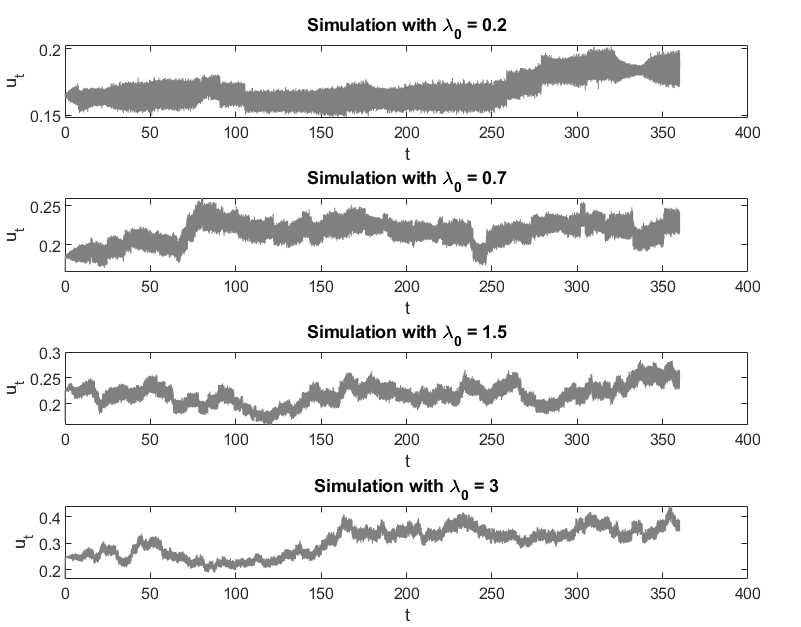
Figure 1: Simulation results of the progression of glioma cell movement under different values of the basal turning rate $\lambda_{0}$, for fixed time steps $h=10^{-4}\,(\text{s})$ and a constant sensitivity to environmental signals parameter $\lambda_{1}=0.08\,(\text{s}^{-1})$.

In Figure 1 and 2, we investigate the temporal evolution of $u_{t}$ under varying values of $\lambda_{0}$ and $\lambda_{1}$ using a time step $h=10^{-4}$ and a simulation duration of $T=360\,(\text{s})$. In particular, the chemoattractant concentration is set to $a=0.5$, the chemorepellent concentration is fixed at $b=0.2$, and all other model parameters are kept constant, as specified in Table 1.
Figure 1 highlights the sensitivity of $u_{t}$ to different values of $\lambda_{0}$, while keeping $\lambda_{1}$ constant at $0.08\,(\text{s}^{-1})$. These observations reveal a direct connection between $\lambda_{0}$ and the amplitude of variation observed in $u_{t}$. As $\lambda_{0}$ decreases, the range of fluctuation is narrower, indicating a more stable and less dynamic behaviour of the glioma cell. Conversely, higher values of $\lambda_{0}$ lead to larger fluctuations, suggesting enhanced cell motility and intensified interactions with the surrounding environment.

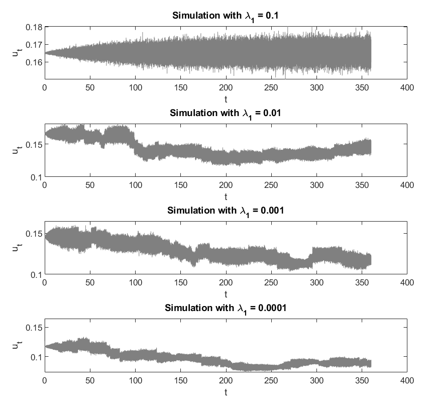
Figure 2: Simulation results of the progression of glioma cell movement under different values of the basal turning rate $\lambda_{0}$, for fixed time steps $h=10^{-4}\,(\text{s})$ and a constant sensitivity to environmental signals parameter $\lambda_{1}=0.08\,(\text{s}^{-1})$.

In Figure 2, we describe the behaviour of $u_{t}$ under the influence of varying the values of $\lambda_{1}$, while $\lambda_{0}$ is set to $0.2\,(\text{s}^{-1})$. As $\lambda_{1}$ is reduced by successive magnitudes, from $10^{-1}\,(\text{s}^{-1})$ to $10^{-4}\,(\text{s}^{-1})$, we observe a consequential decrease in the fluctuation amplitude of $u_{t}$. This implies a stabilising effect on glioma cell migratory behaviour. This stabilisation suggests that $\lambda_{1}$ is a moderator of cellular responsiveness, with higher values enhancing the ability to respond to environmental stimuli. Interestingly, the overall migration activity represented by $u_{t}$ shows robustness to changes in $\lambda_{1}$, reinforcing the idea that $\lambda_{1}$ primarily affects the diversity of migratory responses, rather than the average migratory speed or distance. These simulations suggest a biological interpretation where $\lambda_{1}$ encapsulates the adaptability of glioma cells, with lower values potentially indicating a homogenised, and perhaps less invasive, migration pattern.

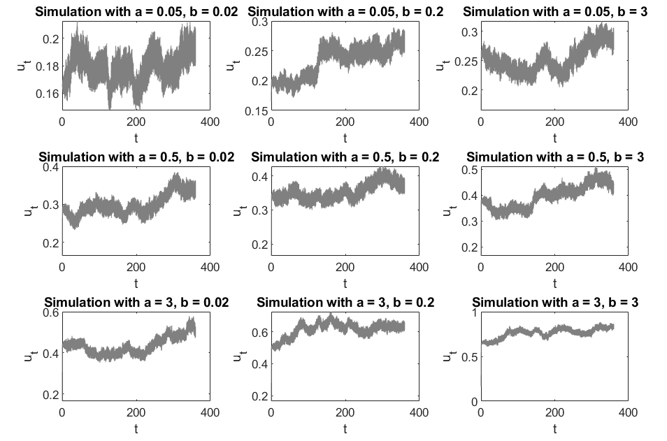
Figure 3: Simulation results for the glioma cell movement for fixed time steps $h=10^{-4}\,(\text{s})$, with $\lambda_{1}=0.08\,(\text{s}^{-1})$ and $\lambda_{0}=0.7\,(\text{s}^{-1})$. The values of $a$ and $b$ are taken within the range in Table 1.

Figures 3 and 4 illustrate the effects of varying the attractant parameter $a$ and the repellent parameter $b$ on the migratory behaviour of glioma cells, represented by the variable $u_{t}$ over a $360\,(\text{s})$ time frame. Figure 3 corresponds to a scenario with a larger fixed value of ${\lambda_{0}=0.7\,(\text{s}^{-1})}$, and Figure 4 represents a scenario with a smaller fixed value of ${\lambda_{0}=0.2\,(\text{s}^{-1})}$. In both cases, the sensitivity to environmental signals parameter $\lambda_{1}$ is fixed to $0.08\,(\text{s}^{-1})$.
The simulation results, presented in Figure 3 with ${\lambda_{0}=0.7\,(\text{s}^{-1})}$, shows a consistent pattern in the overall cellular motion of glioma cells as the attractant and repellent concentrations values changes. In particular, increasing $a$ from $0.05$ to $3$ while keeping $b$ low at $0.02$ (first left column), we observe a pronounced elevation in the fluctuation range of $u_{t}$, suggesting that higher chemoattractant concentrations significantly enhance the mobility of the glioma cell. This enhancement aligns with the chemoattractant’s role as a driving force, pushing the cell towards higher attractant concentrations. Further, when $b$ is increased to $0.2$ with a moderate $a$ value of $0.5$ (second diagonal figure), a substantial rise in $u_{t}$ fluctuations is also notable, indicating increased cell activity possibly due to the combined influence of attractant and repellent factors. The most dynamic cellular behaviour is observed when both attractant and repellent concentrations are simultaneously at their maximum values of 3 (third bottom right figure). The range of $u_{t}$ displays a remarkable expansion, reflecting the heightened motility triggered by the strong conflicting cues from the attractant and repellent. This suggests that the interplay between these external signals leads to a more complex and dynamic pattern of cellular migration.

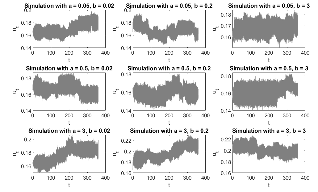
Figure 4: Simulation results for the glioma cell movement for fixed time steps $h=10^{-4}\,(\text{s})$, with $\lambda_{1}=0.08\,(\text{s}^{-1})$ and $\lambda_{0}=0.2\,(\text{s}^{-1})$. The values of $a$ and $b$ are taken within the range in Table 1

In the next test, we set the value of the net motility $\lambda_{0}$ to $0.2\,(\text{s}^{-1})$. This lower value of $\lambda_{0}$ was intentionally chosen to investigate the effect of the attractant and repellent concentrations on the cellular motion while controlling the cell’s intrinsic motility. By reducing $\lambda_{0}$, we are able to isolate the influence of external cues on the cell’s migration pattern, without being overshadowed by the cell’s inherent motility. In Figure 4, the general trends remain consistent; however, the overall values of $u_{t}$ are lower compared to the simulations in Figure 3. This suggests that while $a$ and $b$ are primary determinants of the migratory response, the underlying motility rate $\lambda_{0}$ fundamentally influences the extent of this response. Lower $\lambda_{0}$ seems to suppress the migratory activity, which could imply that the cell’s intrinsic motility is a limiting factor mediating the impact of external cues represented by $a$ and $b$.
These observations collectively indicate that the parameters $a$ and $b$ serve as significant controls over glioma cell migration, modulating the extent and variability of the migratory behaviour. The attractant parameter $a$ appears to promote migration, while the repellent parameter $b$ seems to inhibit it. The role of $\lambda_{0}$ has also been highlighted as a central factor that can enhance or attenuate cellular responses to these signals. These results provide valuable insights into the complex dynamics governing cell migration and highlight the importance of considering both internal and external factors when evaluating the migratory patterns of glioma cells.

6.2.2 Thinned-Splitting Method for PDifMPs

We present here a different approximation for the PDifMP called the Thinned-Splitting Method (TSM), which is a combination of two well-established simulation methods, i.e. the thinning method discussed in Section 3.1, which efficiently simulates the jump times of the underlying jump process, combined with the splitting method, widely used to simulate the stochastic continuous dynamics of the process between jump times [15, 1, 3].
The key idea behind splitting methods is to decompose the right-hand side of the system (54) into explicitly solvable subequations and then to compose the obtained explicit solutions in a proper way. We first start by rewriting the system (54) for $u_{t}=(x_{t},z_{t},v_{t})^{T}$ and $W_{t}=(W^{1}_{t},W^{2}_{t},W^{2}_{t})^{T}$ as

$$du_{t}=\{f^{(1)}(u_{t})dt+G(u_{t})dW_{t}\}+f^{(2)}(u_{t})dt+f^{(3)}(u_{t})dt,$$ (57)

with

$$\begin{array}[]{ll}f^{(1)}(u_{t})=&\begin{pmatrix}\frac{1}{2}z^{2}_{t}x_{t}-bz_{t}x_{t}+az_{t}x_{t}+v_{t}\\ 0\\ 0\end{pmatrix},\\[14.22636pt] f^{(2)}(u_{t})=&\begin{pmatrix}0\\[5.69046pt] -(k^{+}A(x)+k^{-})z_{t}+f^{{}^{\prime}}(A(x))v_{t}A^{{}^{\prime}}(x)\\[5.69046pt] 0\end{pmatrix},\\[14.22636pt] f^{(3)}(u_{t})=&\begin{pmatrix}0\\ 0\\ 0\end{pmatrix},\\[5.69046pt] \end{array}$$

and $G(u_{t})=\begin{pmatrix}z_{t}x_{t}&0&0\\ 0&0&0\\ 0&0&0\end{pmatrix}$.

Hence, we can rewrite the system (54) into the following subsystems

$$du^{[1]}_{t} =f^{(1)}(u_{t})dt+G(u_{t})dW_{t},$$ (58)

$$du^{[2]}_{t} =f^{(2)}(u_{t})dt,$$ (59)

$$du^{[3]}_{t} =f^{(3)}(u_{t})dt.$$ (60)

Equation (58) is not solvable explicitly. Therefore, we split it into two explicitly solvable subsystems of differentiable equations as follows

$$du^{[1,1]}_{t} =\frac{1}{2}z^{2}_{t}u^{[1,1]}_{t}dt+z_{t}u^{[1,1]}dW_{t},$$ (61)

$$du^{[1,2]}_{t} =(-bz_{t}u^{[1,2]}_{t}+az_{t}u^{[1,2]}_{t}+v_{t})dt,$$ (62)

where the subscripts $[1,1]$ and $[1,2]$ correspond to the numbering of the subsystems derived from the first vector $u^{[1]}$. Note that usually the choice of the subsystems is not unique.
Now, all subsystems are explicitly solvable. The SDE (61) has a unique explicit solution given by

$$\psi^{[1]}_{t+h}(u^{[1,1]})=u^{[1,1]}_{t}\exp{\left(z_{t}W_{t}\right)}.$$ (63)

Further, using the fact that the ODE (62) has constant coefficients, it can be solved exactly in closed form, see [19], with

$$\psi^{[2]}_{t+h}(u^{[1,2]})=\exp{(h(-bz_{t}+az_{t}))}u^{[1,2]}_{t}+\frac{\exp{(h(-bz_{t}+az_{t}))}-1}{h(-bz_{t}+az_{t})}hv_{t}.$$ (64)

Therefore, the explicit solution for the first SDE (58), for $t\mapsto t+h$ is given by

$$\psi^{[1]}_{h}(\psi^{[2]}u^{[1]})_{t}=((\exp{(h(-bz_{t}+az_{t}))}u^{[1]}_{t}+\frac{\exp{(h(-bz_{t}+az_{t}))}-1}{h(-bz_{t}+az_{t})}hv_{t})(\exp{\left(z_{t}W_{t}\right)}).$$ (65)

Hence, the explicit solutions $x_{t},z_{t},v_{t}$ are given at time $t$ by

$$\begin{array}[]{ll}\phi^{(1)}_{h}(u_{t})=&\begin{pmatrix}\psi^{[1]}_{t}\big{(}\psi^{[2]}_{t}\big{)}\\ z_{t}\\ v_{t}\end{pmatrix},\\[11.38092pt] \phi^{(2)}_{h}(x_{t})=&\begin{pmatrix}x_{t}\\[8.5359pt] \exp\left(-h(k^{+}A(x)+k^{-})\right)z_{t}+\frac{{\textstyle\exp\left(-h(k^{+}A(x)+k^{-})\right)-1}}{{\textstyle-h(k^{+}A(x)+k^{-})}}hf^{{}^{\prime}}(A(x))v_{t}A^{{}^{\prime}}(x)\\[11.38092pt] v_{t}\end{pmatrix},\\[11.38092pt] \phi^{(3)}_{h}(u(t))=&\begin{pmatrix}x_{t}\\ z_{t}\\ v_{t}\end{pmatrix}.\end{array}$$ (66)

Then, for any time interval $[T_{n},T_{n+1})$ with step size $h$, where ${[T_{n}=t_{0},t_{1},\ldots,t_{M}=T_{n+1})}$, we start with the given initial condition $u_{T_{n}}=(x_{T_{n}},z_{T_{n}},v_{T_{n}}):=\tilde{u}_{0}=(\tilde{x}_{0},\tilde{z}_{0},\tilde{v}_{0})$ and use the Lie-Trotter composition of the flows, see [41], to find the numerical solution ${\tilde{u}_{1},\ldots,\tilde{u}_{m},\ldots,\tilde{u}_{M}}$, such that

$$\tilde{u}_{m+1}=\left(\phi^{(3)}_{h}\circ\phi^{(2)}_{h}\circ\phi^{(1)}_{h}\right)(\tilde{u}_{m})=\phi^{(3)}_{h}\left(\phi^{(2)}_{h}\left(\phi^{(1)}_{h}(\tilde{u}_{m})\right)\right).$$ (67)

Therefore, we have

$$\tilde{u}_{m+1} =\phi^{(3)}_{h}\left(\phi^{(2)}_{h}\begin{pmatrix}\exp{(h(-b\tilde{z}_{m}+a\tilde{z}_{m}))}\tilde{x}_{m}+\frac{{\textstyle\exp{(h(-b\tilde{z}_{m}+a\tilde{z}_{m}))}-1}}{{\textstyle h(-b\tilde{z}_{m}+a\tilde{z}_{m})}}h\tilde{v}_{m}\exp{\left(\tilde{z}_{m}W_{m}\right)}\\[8.5359pt] \tilde{z}_{m}\\[8.5359pt] \tilde{v}_{m}\end{pmatrix}\right),$$ (68)

where, $\tilde{v}_{m}$ is a piecewise constant in each interval of length $t_{m+1}-t_{m}$.

$$\footnotesize{\begin{array}[]{ll}\tilde{u}_{m+1}&=\phi^{(3)}_{h}\begin{pmatrix}\tilde{x}_{m}\\[8.5359pt] \exp\left(-h(k^{+}A(\tilde{x}_{m})+k^{-})\right)\tilde{z}_{m}+\frac{{\textstyle\exp\left(-h(k^{+}A(x)+k^{-})\right)-1}}{{\textstyle-h(k^{+}A(\tilde{x}_{m})+k^{-})}}hf^{{}^{\prime}}(A(\tilde{x}_{m}))\tilde{v}_{m}A^{{}^{\prime}}(\tilde{x}_{m})\\[11.38092pt] \tilde{v}_{m}\end{pmatrix},\end{array}}$$ (69)

$$\footnotesize{\begin{array}[]{ll}\tilde{u}_{m+1}=&\begin{pmatrix}(\exp{(h(-b\tilde{z}_{m}+a\tilde{z}_{m}))}\tilde{x}_{m}+\frac{{\textstyle\exp{(h(-b\tilde{z}_{m}+a\tilde{z}_{m}))}-1}}{{\textstyle h(-b\tilde{z}_{m}+a\tilde{z}_{m}))}}h\tilde{v}_{m}(\exp{\left(\tilde{z}_{m}W_{m}\right)})\\[11.38092pt] \exp\left(-h(k^{+}A(\tilde{x}_{m})+k^{-})\right)\tilde{z}_{m}+\frac{{\textstyle\exp\left(-h(k^{+}A(x)+k^{-})\right)-1}}{{\textstyle-h(k^{+}A(\tilde{x}_{m})+k^{-})}}hf^{{}^{\prime}}(A(\tilde{x}_{m}))\tilde{v}_{m}A^{{}^{\prime}}(\tilde{x}_{m})\\[11.38092pt] \tilde{v}_{m}\end{pmatrix},\end{array}}$$ (70)

where, $\tilde{v}_{m}$ is a piecewise constant in each interval of length $t_{m+1}-t_{m}$.

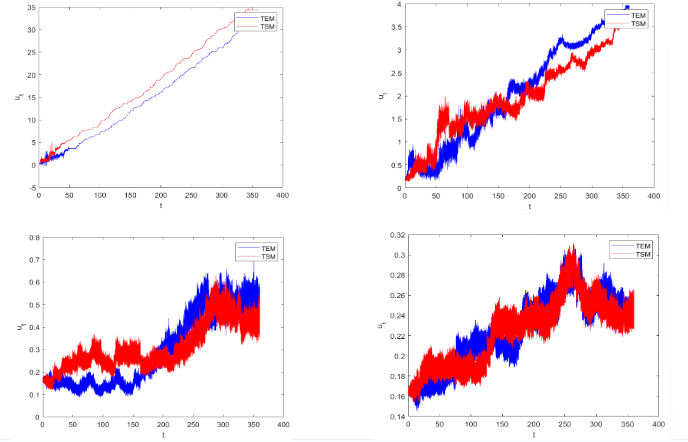
Figure 5: Comparison of the glioma cell movement simulated using the TEM and TSM for different time steps $h$. The parameter values $\lambda_{1}=0.08\,(\text{s}^{-1})$, $\lambda_{0}=0.7\,(\text{s}^{-1})$ were used for both methods. The values of $a$ and $b$ are taken within the range in Table 1

In Figure 5 we present a comparative analysis of the two numerical methods studied above applied to simulate the stochastic process $u_{t}$, which models the movement of glioma cells across varying time steps $h$. In both methods we use the same initial conditions and employ parameter values $\lambda_{0}=0.7\,(\text{s}^{-1})$, $\lambda_{1}=0.08\,(\text{s}^{-1})$, $a=0.5$, and $b=0.2$.
The simulations are executed with time steps $h$ of $0.1,\,0.01,\,0.001$ and $0.0001$ seconds, depicted in the top left, top right, bottom left, and bottom right sub figures, respectively. The TEM method is represented in red, while the TSM is shown in blue.
As $h$ decreases, the results show that the two methods converge towards each other, with the TSM generally exhibiting less variance than the TEM at larger time steps. This is particularly noticeable in the top left sub figure with $h=0.1\,(\text{s})$, where the TEM path is more erratic compared to the TSM. However, as $h$ is reduced, the paths of both methods become increasingly aligned, indicating that the difference between the two methods decreases at finer discretisations.
The convergence of the two methods with decreasing $h$ suggests that the TSM may offer a more stable solution at coarser time steps, potentially due to better handling of the stochasticity and jumps in the model.
In contrast, the TEM method appears to be more sensitive to the size of $h$, with its greater variability at larger time steps potentially reflecting a higher numerical error or less accuracy in capturing the jump dynamics. This sensitivity diminishes with smaller $h$, which aligns with the expected increase in numerical precision as the time step approaches zero.
In conclusion, the TSM seems to be more robust across varying time steps, particularly at larger $h$, while the TEM method requires smaller time steps to achieve similar accuracy, which has implications for computational efficiency and accuracy in simulations of glioma cell movement. This evaluation provides valuable insights for selecting appropriate numerical schemes for stochastic simulations in biological systems, where the trade-off between computational cost and accuracy is often a critical consideration.

7 Discussion

The numerical simulation of PDifMPs poses a significant challenge due to their complex dynamics and the difficulty in obtaining explicit expressions for their characteristics. Although some methods have been proposed for simulating generalised stochastic hybrid systems, these methods often lack a general framework for handling PDifMPs. Additionally, they typically do not investigate the convergence properties of the employed methods, see [12].
To bridge this gap, we propose two novel numerical approaches for simulating PDifMPs; the Thinned Euler-Maruyama (TEM) method for a general framework, and the Thinned Splitting Method (TSM) for a specific model, as detailed in Section 6. Further, we have conducted a detailed analysis of both the mean square and weak convergence of the TEM method.
To illustrate the performance of both the TEM and the TSM, we applied these methods to model the motion of a glioma cell at the microscopic level, and we compare the trajectories generated by each simulation. On the one hand, our numerical method allow us to explore how microscopic parameters, such as the net cell motility and environmental signals affect cellular behaviour, on the other hand, our comparative study reveals that TSM demonstrates enhanced stability in simulating the dynamics of glioma cells, highlighting the effectiveness of using a tailored approach.
Looking towards future research directions, we propose further numerical analysis of the TEM and the TSM to further assess their efficacy and scalability. In particular, the innovative combination of thinning and splitting methods in simulating PDifMPs warrants further exploration, especially regarding the unique jump-adapted time discretisation scheme. This exploration would significantly contribute to our understanding of convergence properties in the context of PDifMPs and pave the way for more sophisticated and efficient numerical simulations.

Declaration of competing interest

The authors declare that they have no known competing financial interests or personal relationships that could have appeared to influence the work reported in this paper.

Funding

This work was supported by the Austrian Science Fund (FWF): W1214-N15, project DK14, as well as by the strategic program ”Innovatives OÖ 2010 plus” by the Upper Austrian Government.

Appendix A

Proof.

Lemma 3.2
Let $\phi(t,(y_{1},v))$ and $\phi(t,(y_{1},v))$ satisfy the integral form (2). We have,

$$\lvert\phi(t,(y_{1},v))-\phi(t,(y_{2},v))\rvert^{2}=\lvert(y_{1}-y_{2})+\int_{0}^{t}\big{(}b(\phi(s,(y_{1},v)),v)-b(\phi(s,(y_{2},v)),v)\big{)}ds+\\ \int_{0}^{t}\big{(}\sigma(\phi(s,(y_{1},v)),v)-\sigma(\phi(s,(y_{2},v)),v)\big{)}dW_{s}\rvert^{2}.$$

Using the triangle inequality, the Hölder’s inequality and the Itô isometry, we obtain

$$\lvert\phi(t,(y_{1},v))-\phi(t,(y_{2},v))\rvert^{2} \leq\lvert(y_{1}-y_{2})\rvert^{2}+\lvert\int_{0}^{t}\big{(}b(\phi(s,(y_{1},v)),v)-b(\phi(s,(y_{2},v)),v)\big{)}ds\rvert^{2}$$

$$\qquad\qquad+\lvert\int_{0}^{t}\big{(}\sigma(\phi(s,(y_{1},v)),v)-\sigma(\phi(s,(y_{2},v)),v)\big{)}dW_{s}\rvert^{2}$$

$$\leq\lvert(y_{1}-y_{2})\rvert^{2}+\int_{0}^{t}\lvert\big{(}b(\phi(s,(y_{1},v)),v)-b(\phi(s,(y_{2},v)),v)\big{)}\rvert^{2}ds$$

$$\qquad\qquad+\int_{0}^{t}\lvert\big{(}\sigma(\phi(s,(y_{1},v)),v)-\sigma(\phi(s,(y_{2},v)),v)\big{)}\rvert^{2}d{s}.$$

Using the Lipschitz continuity of the coefficients $b$ and $\sigma$ as given in (3), we get

$$\lvert\phi(t,(y_{1},v))-\phi(t,(y_{2},v))\rvert^{2} \leq\lvert(y_{1}-y_{2})\rvert^{2}+K_{1}\int_{0}^{t}\lvert\phi(s,(y_{1},v))-\phi(s,(y_{2},v))\rvert^{2}ds$$

$$\qquad\qquad+K_{2}\int_{0}^{t}\lvert\phi(s,(y_{1},v))-\phi(s,(y_{2},v))\rvert^{2}ds$$

$$\leq\lvert(y_{1}-y_{2})\rvert^{2}+2K_{1}\int_{0}^{t}\lvert\phi(s,(y_{1},v))-\phi(s,(y_{2},v))\rvert^{2}ds.$$

Since we start with deterministic initial values $y_{1}$, $y_{2}$, using Gronwall’s inequality, we have

$$\mathbb{E}[\sup_{t\in[0,T]}\lvert\phi(t,(y_{1},v))-\phi(t,(y_{2},v))\rvert^{2}] \leq\mathbb{E}[\sup_{t\in[0,T]}\lvert y_{1}-y_{2}\rvert^{2}]+2K_{1}\int_{0}^{t}\mathbb{E}[\sup_{t\in[0,T]}\lvert\phi(s,(y_{1},v))-\phi(s,(y_{2},v))\rvert^{2}]ds.$$

$$\leq K_{3}\lvert y_{1}-y_{2}\rvert^{2}e^{2K_{2}T},$$

$$\leq\lvert y_{1}-y_{2}\rvert^{2}e^{C_{1}T}.$$

∎

Appendix B

Lemma 1.

Let $\mathbf{V}$ be a finite set, with $|\mathbf{V}|$ representing the cardinal number of $\mathbf{V}$ and $\kappa_{i}$ indicating the elements of $\mathbf{V}$ for $i=1,2,\ldots,|\mathbf{V}|$. Let $p_{i}$ and $\overline{p}_{i}$, $1\leq i\leq|\mathbf{V}|$, be two probability distributions on $\mathbf{V}$. We define the cumulative probabilities for these distributions at each index $j$ as $a_{j}=\sum_{i=1}^{j}p_{i}$ and $\overline{a}_{j}=\sum_{i=1}^{j}\overline{p}_{i}$, respectively, with the initial values set as $a_{0}=\overline{a}_{0}:=0$. Let $X$ and $\overline{X}$ be two $\mathbf{V}$-valued random variables defined by

$$X:=G(\mathcal{U}),\qquad\overline{X}:=\overline{G}(\mathcal{U}),$$

where

$$\mathcal{U}\sim\mathcal{U}([0,1]),\qquad G(u)=\sum_{j=1}^{|\mathbf{V}|}\kappa_{j}\mathbbm{1}_{a_{j-1}<u\leq a_{j}}\quad\text{and}\quad\overline{G}(u)=\sum_{j=1}^{|\mathbf{V}|}\kappa_{j}\mathbbm{1}_{\overline{a}_{j-1}<u\leq\overline{a}_{j}}\quad\text{for all}\,\,{u\in[0,1]}.$$

Then, we have

$$\mathbb{P}(X\neq\overline{X})\leq\sum_{j=1}^{|\mathbf{V}|-1}\left|a_{j}-\overline{a}_{j}\right|.$$

Proof.

We refer to [37] for the proof of Lemma 1. ∎

References

- [1] Markus Ableidinger, Evelyn Buckwar and Harald Hinterleitner “A stochastic version of the Jansen and Rit neural mass model: analysis and numerics” In The Journal of Mathematical Neuroscience 7.1 SpringerOpen, 2017, pp. 1–35
- [2] Iman Aganj et al. “A Hough transform global probabilistic approach to multiple-subject diffusion MRI tractography” In Medical image analysis 15.4 Elsevier, 2011, pp. 414–425
- [3] Alfonso Alamo and Jesús María Sanz-Serna “A technique for studying strong and weak local errors of splitting stochastic integrators” In SIAM Journal on Numerical Analysis 54.6 SIAM, 2016, pp. 3239–3257
- [4] Marine Aubert et al. “A cellular automaton model for the migration of glioma cells” In Physical biology 3.2 IOP Publishing, 2006, pp. 93
- [5] Nicholas A Baran, George Yin and Chao Zhu “Feynman-Kac formula for switching diffusions: connections of systems of partial differential equations and stochastic differential equations” In Advances in Difference Equations 2013.1 SpringerOpen, 2013, pp. 1–13
- [6] Julien Bect “Processus de Markov diffusifs par morceaux: outils analytiques et numériques”, 2007
- [7] Howard C Berg and Douglas A Brown “Chemotaxis in Escherichia Coli analysed by three-dimensional tracking” In Nature 239.5374 Nature Publishing Group, 1972, pp. 500–504
- [8] Andrea Bertazzi, Joris Bierkens and Paul Dobson “Approximations of piecewise deterministic Markov processes and their convergence properties” In Stochastic Processes Appl. 154, 2022, pp. 91–153 DOI: 10.1016/j.spa.2022.09.004
- [9] Joris Bierkens, Paul Fearnhead and Gareth Roberts “The zig-zag process and super-efficient sampling for Bayesian analysis of big data”, 2019
- [10] Joris Bierkens et al. “Piecewise deterministic Markov processes for scalable Monte Carlo on restricted domains” In Statistics & Probability Letters 136 Elsevier, 2018, pp. 148–154
- [11] HAP Blom “From piecewise deterministic to piecewise diffusion Markov processes” In Proceedings of the 27th IEEE Conference on Decision and Control, 1988, pp. 1978–1983 IEEE
- [12] Henk AP Blom, Hao Ma and GJ Bert Bakker “Interacting particle system-based estimation of reach probability for a generalized stochastic hybrid system” In IFAC-PapersOnLine 51.16 Elsevier, 2018, pp. 79–84
- [13] Alexandre Bouchard-Côté, Sebastian J Vollmer and Arnaud Doucet “The bouncy particle sampler: A nonreversible rejection-free Markov chain Monte Carlo method” In Journal of the American Statistical Association 113.522 Taylor & Francis, 2018, pp. 855–867
- [14] Evelyn Buckwar and Martin G Riedler “An exact stochastic hybrid model of excitable membranes including spatio-temporal evolution” In Journal of mathematical biology 63.6 Springer, 2011, pp. 1051–1093
- [15] Evelyn Buckwar, Adeline Samson, Massimiliano Tamborrino and Irene Tubikanec “A splitting method for SDEs with locally Lipschitz drift: Illustration on the FitzHugh-Nagumo model” In Applied Numerical Mathematics 179 Elsevier, 2022, pp. 191–220
- [16] Manuela L Bujorianu and John Lygeros “Reachability questions in piecewise deterministic Markov processes” In International Workshop on Hybrid Systems: Computation and Control, 2003, pp. 126–140 Springer
- [17] Manuela L Bujorianu and John Lygeros “Toward a general theory of stochastic hybrid systems” In Stochastic hybrid systems Springer, 2006, pp. 3–30
- [18] SERGIO BLANES1 FERNANDO CASAS and ANDER MURUA “Splitting and composition methods in the numerical integration of differential equations” In BOLETÍN NUMERO 45 Diciembre 2008, 2008, pp. 89
- [19] Zhengdao Chen, Baranidharan Raman and Ari Stern “Structure-Preserving Numerical Integrators for Hodgkin–Huxley-Type Systems” In SIAM Journal on Scientific Computing 42.1 SIAM, 2020, pp. B273–B298
- [20] M.. Chicoine and D.. Silbergeld “Assessment of brain tumor cell motility in vivo and in vitro” In Journal of Neurosurgery 82.4 Journal of Neurosurgery Publishing Group, 1995, pp. 615–622 DOI: 10.3171/jns.1995.82.4.0615
- [21] Bertrand Cloez et al. “Probabilistic and piecewise deterministic models in biology” In ESAIM: Proceedings and Surveys 60 EDP Sciences, 2017, pp. 225–245
- [22] Martina Conte, Luca Gerardo-Giorda and Maria Groppi “Glioma invasion and its interplay with nervous tissue and therapy: A multiscale model” In Journal of theoretical biology 486 Elsevier, 2020, pp. 110088
- [23] Mark HA Davis “Piecewise-deterministic Markov processes: A general class of non-diffusion stochastic models” In Journal of the Royal Statistical Society: Series B (Methodological) 46.3 Wiley Online Library, 1984, pp. 353–376
- [24] Alain Durmus, Arnaud Guillin and Pierre Monmarché “Piecewise deterministic Markov processes and their invariant measures” In Annales de l’Institut Henri Poincaré, Probabilités et Statistiques 57.3, 2021, pp. 1442–1475 Institut Henri Poincaré
- [25] Christian Engwer, Alexander Hunt and Christina Surulescu “Effective equations for anisotropic glioma spread with proliferation: a multiscale approach and comparisons with previous settings” In Mathematical medicine and biology: a journal of the IMA 33.4 Oxford University Press, 2016, pp. 435–459
- [26] Christian Engwer, Markus Knappitsch and Christina Surulescu “A multiscale model for glioma spread including cell-tissue interactions and proliferation” In Mathematical Biosciences & Engineering 13.2 American Institute of Mathematical Sciences, 2016, pp. 443
- [27] Christian Engwer, Thomas Hillen, Markus Knappitsch and Christina Surulescu “Glioma follow white matter tracts: a multiscale DTI-based model” In Journal of mathematical biology 71.3 Springer, 2015, pp. 551–582
- [28] Carl Graham and Denis Talay “Stochastic simulation and Monte Carlo methods: mathematical foundations of stochastic simulation” Springer Science & Business Media, 2013
- [29] Hana LP Harpold, Ellsworth C Alvord Jr and Kristin R Swanson “The evolution of mathematical modeling of glioma proliferation and invasion” In Journal of Neuropathology & Experimental Neurology 66.1 American Association of Neuropathologists, Inc., 2007, pp. 1–9
- [30] Thomas Hillen “On the -moment closure of transport equations: The Cattaneo approximation” In Discrete & Continuous Dynamical Systems-B 4.4 American Institute of Mathematical Sciences, 2004, pp. 961
- [31] Thomas Hillen and Kevin J Painter “Transport and anisotropic diffusion models for movement in oriented habitats” In Dispersal, individual movement and spatial ecology Springer, 2013, pp. 177–222
- [32] Alexander Hunt “DTI-based multiscale models for glioma invasion”, 2018
- [33] Hiroshi Ishijima and Masaki Uchida “The regime switching portfolios” In Asia-Pacific Financial Markets 18 Springer, 2011, pp. 167–189
- [34] Peter Kritzer, Gunther Leobacher, Michaela Szölgyenyi and Stefan Thonhauser “Approximation methods for piecewise deterministic Markov processes and their costs” In Scandinavian Actuarial Journal 2019.4 Taylor & Francis, 2019, pp. 308–335
- [35] Douglas A Lauffenburger and Jennifer Linderman “Receptors: models for binding, trafficking, and signaling” Oxford University Press, 1996
- [36] Vincent Lemaire, Michèle Thieullen and Nicolas Thomas “Exact simulation of the jump times of a class of piecewise deterministic Markov processes” In Journal of Scientific Computing 75.3 Springer, 2018, pp. 1776–1807
- [37] Vincent Lemaire, Michèle Thieullen and Nicolas Thomas “Thinning and Multilevel Monte Carlo for Piecewise Deterministic (Markov) Processes. Application to a stochastic Morris-Lecar model” In Advances in Applied Probability 52.1 Cambridge University Press, 2020, pp. 138–172
- [38] PA W Lewis and Gerald S Shedler “Simulation of nonhomogeneous Poisson processes by thinning” In Naval Research Logistics Quarterly 26.3 Wiley Online Library, 1979, pp. 403–413
- [39] Roland Malhamé “A jump-driven Markovian electric load model” In Advances in Applied Probability 22.3 Cambridge University Press, 1990, pp. 564–586
- [40] Xuerong Mao “Stochastic differential equations and applications” Elsevier, 2007
- [41] Robert I McLachlan and G Reinout W Quispel “Splitting methods” In Acta Numerica 11 Cambridge University Press, 2002, pp. 341–434
- [42] Amira Meddah, Martina Conte and Evelyn Buckwar “A stochastic hierarchical model for low grade glioma evolution” In Journal of Mathematical Biology, 2023
- [43] Hiroko Ohgaki “Epidemiology of brain tumors” In Cancer Epidemiology: Modifiable Factors Springer, 2009, pp. 323–342
- [44] Gilles Pagès “Numerical probability” In Universitext, Springer Springer, 2018
- [45] KJ Painter and Thomas Hillen “Mathematical modelling of glioma growth: the use of diffusion tensor imaging (DTI) data to predict the anisotropic pathways of cancer invasion” In Journal of theoretical biology 323 Elsevier, 2013, pp. 25–39
- [46] Khashayar Pakdaman, Michele Thieullen and Gilles Wainrib “Fluid limit theorems for stochastic hybrid systems with application to neuron models” In Advances in Applied Probability 42.3 Cambridge University Press, 2010, pp. 761–794
- [47] WP Petersen “A general implicit splitting for stabilizing numerical simulations of Itô stochastic differential equations” In SIAM journal on numerical analysis 35.4 SIAM, 1998, pp. 1439–1451
- [48] Eckhard Platen, Nicola Bruti-Liberati, Eckhard Platen and Nicola Bruti-Liberati “Jump-Adapted Strong Approximations” In Numerical Solution of Stochastic Differential Equations with Jumps in Finance Springer, 2010, pp. 347–388
- [49] Martin G Riedler “Almost sure convergence of numerical approximations for piecewise deterministic Markov processes” In Journal of Computational and Applied Mathematics 239 Elsevier, 2013, pp. 50–71
- [50] Tony Shardlow “Splitting for dissipative particle dynamics” In SIAM Journal on Scientific computing 24.4 SIAM, 2003, pp. 1267–1282
- [51] M. Sidani et al. “Cofilin determines the migration behavior and turning frequency of metastatic cancer cells” In The Journal of Cell Biology 179.4 Rockefeller University Press, 2007, pp. 777–791 DOI: 10.1083/jcb.200707009
- [52] Abhyudai Singh and Joao P Hespanha “Stochastic hybrid systems for studying biochemical processes” In Philosophical Transactions of the Royal Society A: Mathematical, Physical and Engineering Sciences 368.1930 The Royal Society Publishing, 2010, pp. 4995–5011
- [53] Kristin R Swanson, Ellsworth C Alvord Jr and JD Murray “A quantitative model for differential motility of gliomas in grey and white matter” In Cell proliferation 33.5 Wiley Online Library, 2000, pp. 317–329
- [54] Denis Talay and Luciano Tubaro “Expansion of the global error for numerical schemes solving stochastic differential equations” In Stochastic analysis and applications 8.4 Taylor & Francis, 1990, pp. 483–509
- [55] Romain Veltz “A new twist for the simulation of hybrid systems using the true jump method” In arXiv preprint arXiv:1504.06873, 2015
- [56] G Yin and Chao Zhu “Properties of solutions of stochastic differential equations with continuous-state-dependent switching” In Journal of Differential Equations 249.10 Elsevier, 2010, pp. 2409–2439
- [57] G George Yin and Chao Zhu “Hybrid switching diffusions: properties and applications” Springer Science & Business Media, 2009
- [58] Chenggui Yuan and Xuerong Mao “Convergence of the Euler–Maruyama method for stochastic differential equations with Markovian switching” In Mathematics and Computers in Simulation 64.2 Elsevier, 2004, pp. 223–235