A Lagrange-Newton Approach
to Smoothing-and-Mapping

Abstract

In this report we explore the application of the Lagrange-Newton method to the SAM (smoothing-and-mapping) problem in mobile robotics. In Lagrange-Newton SAM, the angular component of each pose vector is expressed by orientation vectors and treated through Lagrange constraints. This is different from the typical Gauss-Newton approach where variations need to be mapped back and forth between Euclidean space and a manifold suitable for rotational components. We derive equations for five different types of measurements between robot poses: translation, distance, and rotation from odometry in the plane, as well as home-vector angle and compass angle from visual homing. We demonstrate the feasibility of the Lagrange-Newton approach for a simple example related to a cleaning robot scenario.

1 Introduction

Smoothing-and-mapping (SAM) is a fairly modern approach to building graph-based maps of the environment; a tutorial is given by Grisetti et al. (2010) (see also the tutorial on Newton-type methods with applications in graph-based SLAM by Toussaint (2017)). Following the tutorial by Grisetti et al. (2010), the SAM problem (1) is solved in a Gauss-Newton framework and (2) involves transformations between manifolds for the rotational components. In the Gauss-Newton framework, error vectors (between true and expected measurements) are approximated to first order by a Taylor expansion, thus the resulting scalar error terms are second-order equations. A Newton descent is then performed based on the approximated Hessian (computed from the Jacobian) in these equations.

However, while the Gauss-Newton framework allows for straightforward derivations, it suffers from a drawback with respect to rotational cost functions: In the quadratic approximation of the scalar error functions, the cyclic character of angular terms is lost. Therefore, to handle rotational components (e.g. pose angles), variations need to be transformed between the Euclidean space (assumed by the Gauss-Newton approach) and a manifold suitable for the rotational components (Grisetti et al., 2010). Deriving and understanding these transformations is demanding.

Here we explore a different approach to the SAM problem where we (1) perform a full Newton descent and (2) treat rotational components by constraints in a Lagrange-Newton framework. For the Newton descent, we compute the exact Hessian, not an approximation. Rotational components are described by orientation vectors with the unit-length constraint expressed by Lagrange constraints. Lagrange multipliers become part of the state vector. Note that a Newton descent is not only faster than a gradient descent, but indispensable if the Lagrange multipliers are included since in this case the extreme point is always a saddle; multiplication of the gradient by the inverse Hessian turns the saddle into an attractor.

The core idea explored here is to express rotational components through orientation vectors (with unit length) instead of angles. In this way, the problem space remains Euclidean. Equality constraints expressing the unit-length property are handled by the Lagrange-multiplier method (2). The fact that we apply Newton’s method with an exact computation of the Hessian (1) is currently a necessity since we didn’t see whether and how the Gauss-Newton framework would be compatible with this idea. It is also not clear whether computing the exact Hessian would improve the performance of the method compared to the approximated Hessian. An obvious disadvantage is the preparatory effort required to symbolically compute the exact Hessian. Moreover, the algorithmic solution of the Lagrange-Newton iteration is complicated by the saddle-point property mentioned above (e.g. for choosing a criterion for the line-search).

We apply our Lagrange-Newton approach to the problem of navigation in the plane. We define five cost functions: translation, distance, and rotation error derived from an odometry model, and home-vector and compass error related to a visual homing method. We also explore different variants of the three rotational cost functions (rotation, home-vector, and compass error). The visual homing method determines two estimates from a pair of panoramic views captured at two different locations: the direction (home vector) from one capture point to the other, and the azimuthal rotation between the views (compass). This is the approach used in our previous work on cleaning robot navigation (Möller et al., 2013; Gerstmayr-Hillen et al., 2013). Also our exploratory simulation is related to the cleaning-robot scenario.

After introducing the notation in section 2, we define planar orientation vectors which express angular terms and explore their properties in section 3. The five cost functions are defined in section 4. The first- and second-order derivatives required for the Newton method are determined in section 5. All derivatives are combined in the terms required for the Lagrange-Newton descent in section 6. Section 7 describes the preliminary experiments and their results. Conclusions are presented in section 8.

2 Notation

The two poses paired in a measurement are called “first point/pose” and “second point/pose” here.

Dimensions

$N$: number of poses, $2\leq N$

$M_{o}$: number of odometry measurements (translation, distance, rotation), $1\leq M_{o}$

$M_{h}$: number of homing measurements (home vector, compass), $1\leq M_{h}$

Odometry Measurement

$\mathbf{C}$: odometry covariance (in robot coordinates of first point), symmetric, $3\times 3$

$\mathbf{T}$: translatory covariance (in robot coordinates of first point), symmetric, $2\times 2$

$\sigma$: angular standard deviation of odometry, scalar, $1\times 1$

$\sigma_{e}$: standard deviation of odometry distance, scalar, $1\times 1$

$\mathbf{b}$: cross-covariance terms in odometry covariance matrix, arbitrary, $2\times 1$

$\mathbf{r}$: odometry translation vector (in robot coordinates of first point), arbitrary, $2\times 1$

$\varrho$: odometry distance (length of translation vector), scalar, $1\times 1$

$\mathbf{q}$: odometry orientation change vector, arbitrary, $2\times 1$

$\mathbf{Q}$: odometry orientation change matrix, orthogonal, $2\times 2$

Homing Measurement

$\boldsymbol{\alpha}$: home orientation vector (in robot coordinates), arbitrary, $2\times 1$

$\boldsymbol{A}$: home orientation matrix (in robot coordinates), orthogonal, $2\times 2$

$\sigma_{h}$: standard deviation of home-vector measurement, scalar, $1\times 1$

$\boldsymbol{\psi}$: compass orientation vector (in robot coordinates), arbitrary, $2\times 1$

$\boldsymbol{\Psi}$: compass orientation matrix (in robot coordinates), orthogonal, $2\times 2$

$\sigma_{c}$: standard deviation of compass measurement, scalar, $1\times 1$

Pose Estimates

$\boldsymbol{\delta}$: position change (estimate, in world coordinates), arbitrary, $2\times 1$

$\boldsymbol{\delta}_{0}$: unit vector of $\boldsymbol{\delta}$, arbitrary, $2\times 1$

$\mathbf{d}$: position change (estimate, in robot coordinates of first point), arbitrary, $2\times 1$

$\mathbf{x}$: position of first robot pose (estimate, in world coordinates), arbitrary, $2\times 1$

$\mathbf{u}$: orientation vector of first robot pose (estimate, in world coordinates), arbitrary, $2\times 1$

$\mathbf{U}$: orientation matrix of first robot pose (estimate), square, $2\times 2$

$\mathbf{p}$: first robot pose (estimate, in world coordinates), arbitrary, $4\times 1$

$\mathbf{x}^{\prime}$: position of second robot pose (estimate, in world coordinates), arbitrary, $2\times 1$

$\mathbf{u}^{\prime}$: orientation vector of second robot pose (estimate, in world coordinates), arbitrary, $2\times 1$

$\mathbf{U}^{\prime}$: orientation matrix of second robot pose (estimate), square, $2\times 2$

$\mathbf{p}^{\prime}$: second robot pose (estimate, in world coordinates), arbitrary, $4\times 1$

Cost Functions

$e$: distance odometry cost function, scalar, $1\times 1$

$f$: translatory odometry cost function, scalar, $1\times 1$

$g$: rotatory odometry cost function 1, scalar, $1\times 1$

$\bar{g}$: rotatory odometry cost function 2, scalar, $1\times 1$

$h$: home-vector cost function 1, scalar, $1\times 1$

$\bar{h}$: home-vector cost function 2, scalar, $1\times 1$

$c$: compass cost function 1, scalar, $1\times 1$

$\bar{c}$: compass cost function 2, scalar, $1\times 1$

$\gamma$: weight factor for orientation cost terms, scalar, $1\times 1$

${\lambda}_{i}$: Lagrange multipliers, scalar, $1\times 1$

$\boldsymbol{\lambda}$: vector of Lagrange multipliers, arbitrary, $(N-1)\times 1$

$w$: Lagrange constraint term on orientation vectors, scalar, $1\times 1$

$l$: inner constraint term on orientation vectors, scalar, $1\times 1$

$L$: Lagrangian, scalar, $1\times 1$

$F$: sum of cost functions in Lagrangian, scalar, $1\times 1$

$s$: generic rotational cost function 1, scalar, $1\times 1$

$\bar{s}$: generic rotational cost function 2, scalar, $1\times 1$

$\varphi$: angle, scalar, $1\times 1$

$\boldsymbol{\Phi}$: orientation matrix, orthogonal, $2\times 2$

Newton Method

$\mathbf{H}$: total Hessian (without first pose), symmetric, $(5N-5)\times(5N-5)$

$\mathbf{g}$: total gradient vector (without first pose), arbitrary, $(5N-5)\times 1$

$\boldsymbol{\Delta}\mathbf{s}$: state change vector (without first pose), arbitrary, $(5N-5)\times 1$

$\mathbf{R}$: regularization matrix, diagonal, $(5N-5)\times(5N-5)$

$\eta_{W}$: Levenberg-Marquardt factor (for core of bordered Hessian), scalar, $1\times 1$

$\eta_{A}$: Levenberg-Marquardt factor (for border of bordered Hessian), scalar, $1\times 1$

Other

$\mathfrak{d}$: Kronecker delta, scalar, $1\times 1$

$\mathbf{M}$: transformation matrix, symmetric, $2\times 2$

$\mathbf{N}$: transformation matrix, symmetric, $2\times 2$

$\boldsymbol{\Omega}$: operator which turns orientation vector into orientation matrix, square, $2\times 2$

$\overline{\boldsymbol{\Omega}}$: operator with negated second column w.r.t. $\boldsymbol{\Omega}$, symmetric, $2\times 2$

$\mathbf{x}$: general vector, arbitrary, $2\times 1$

$\mathbf{y}$: general vector, arbitrary, $2\times 1$

$\mathbf{z}$: general vector, arbitrary, $2\times 1$

$\mathbf{v}$: general vector, arbitrary, $2\times 1$

$t_{1}$: configuration parameter, scalar, $1\times 1$

$\bar{t}_{1}$: configuration parameter, scalar, $1\times 1$

3 Orientation Vectors

In Lagrange-Newton SAM, angles are described by unit “orientation vectors”. In this way, the problem space remains Euclidean. Unit-length constraints on the orientation vectors are handled by constraint terms in the Lagrangian. To give an example of an orientation vector: If the orientation of the first robot pose is described by an angle $\Theta$, the orientation vector $\mathbf{u}$ is

$$\mathbf{u}=\begin{pmatrix}u_{1}\\ u_{2}\end{pmatrix}=\begin{pmatrix}\cos\Theta\\ \sin\Theta\end{pmatrix}.$$ (1)

Note that there are constant unit vectors (e.g. those relating to measurements) and variable vectors which should approach unit length by the constraints applied in the Lagrange-Newton descent ($\mathbf{u}$ is actually an example of the latter class: it is only initially computed as a unit vector from the angle $\Theta$ and then updated in the Lagrange-Newton descent).

To form a Cartesian right-handed coordinate system where $\mathbf{u}$ is the first axis, the vector perpendicular to $\mathbf{u}$ can be obtained from

$$\begin{pmatrix}-u_{2}\\ u_{1}\end{pmatrix}.$$ (2)

The orthogonal (or approximately orthogonal) “orientation matrix” describing the coordinate system formed by the two vectors is expressed by the operator $\boldsymbol{\Omega}$ applied to an orientation vector:

$$\mathbf{U} =\boldsymbol{\Omega}\left(\mathbf{u}\right)=\begin{pmatrix}u_{1}&-u_{2}\\ u_{2}&u_{1}\end{pmatrix}.$$ (3)

To add angles, one of the angles is turned into an (approximately) orthogonal rotation matrix, namely the corresponding orientation matrix. For example, if we want to add the odometry orientation change $\varphi$ (described by orientation vector $\mathbf{q}$ and the orientation matrix $\mathbf{Q}$) to the orientation angle $\Theta$ (described by orientation vector $\mathbf{u}$), we can write $\mathbf{Q}\mathbf{u}$.

To give a numerical example: for $\varphi=30^{\circ}$, $\Theta=60^{\circ}$ we get

$$\mathbf{q} =\begin{pmatrix}\frac{1}{2}\,\sqrt{3}\\ \frac{1}{2}\,\end{pmatrix}$$ (4)

$$\mathbf{Q} =\boldsymbol{\Omega}\left(\mathbf{q}\right)=\begin{pmatrix}\frac{1}{2}\,\sqrt{3}&-\frac{1}{2}\,\\ \frac{1}{2}\,&\frac{1}{2}\,\sqrt{3}\end{pmatrix}$$ (5)

$$\mathbf{u} =\begin{pmatrix}\frac{1}{2}\,\\ \frac{1}{2}\,\sqrt{3}\end{pmatrix}$$ (6)

$$\mathbf{Q}\mathbf{u} =\begin{pmatrix}\frac{1}{2}\,\sqrt{3}\frac{1}{2}\,+\left(-\frac{1}{2}\,\frac{1}{2}\,\sqrt{3}\right)\\ \frac{1}{2}\,\frac{1}{2}\,+\frac{1}{2}\,\sqrt{3}\frac{1}{2}\,\sqrt{3}\end{pmatrix}=\begin{pmatrix}\frac{1}{4}\,\sqrt{3}+\left(-\frac{1}{4}\,\sqrt{3}\right)\\ \frac{1}{4}\,+\frac{1}{4}\,\sqrt{3}\sqrt{3}\end{pmatrix}=\begin{pmatrix}0\\ 1\end{pmatrix},$$ (7)

which is the orientation vector for the angle sum $\varphi+\Theta=90^{\circ}$.

In the derivatives, a second operator appears which is labeled $\overline{\boldsymbol{\Omega}}$ (see below). It differs from $\boldsymbol{\Omega}$ in that the second column is multiplied by $-1$. Applied to $\mathbf{u}$ it would give

$$\overline{\boldsymbol{\Omega}}\left(\mathbf{u}\right) =\begin{pmatrix}u_{1}&u_{2}\\ u_{2}&-u_{1}\end{pmatrix}.$$ (8)

For transformations, we introduce the symmetric matrices $\mathbf{M}$ and $\mathbf{N}$

$$\mathbf{M} =\begin{pmatrix}1&0\\ 0&-1\end{pmatrix}$$ (9)

$$\mathbf{N} =\begin{pmatrix}0&1\\ 1&0\end{pmatrix}$$ (10)

such that we can write

$$\mathbf{U} =\boldsymbol{\Omega}\left(\mathbf{u}\right)=\begin{pmatrix}\mathbf{u}^{T}\mathbf{M}\\ \mathbf{u}^{T}\mathbf{N}\end{pmatrix}$$ (11)

$$\mathbf{U}^{T} =\left(\boldsymbol{\Omega}\left(\mathbf{u}\right)\right)^{T}=\begin{pmatrix}\mathbf{M}\mathbf{u}&\mathbf{N}\mathbf{u}\end{pmatrix}.$$ (12)

We generally see that, for any two-dimensional vectors $\mathbf{x}$, $\mathbf{y}$, and $\mathbf{z}$,

$$\boldsymbol{\Omega}\left(\mathbf{z}\right) =\begin{pmatrix}\mathbf{z}^{T}\mathbf{M}\\ \mathbf{z}^{T}\mathbf{N}\end{pmatrix}=\begin{pmatrix}z_{1}&-z_{2}\\ z_{2}&z_{1}\end{pmatrix}$$ (13)

$$\left(\boldsymbol{\Omega}\left(\mathbf{z}\right)\right)^{T} =\begin{pmatrix}\mathbf{M}\mathbf{z}&\mathbf{N}\mathbf{z}\end{pmatrix}$$ (14)

$$\overline{\boldsymbol{\Omega}}\left(\mathbf{z}\right) =\boldsymbol{\Omega}\left(\mathbf{z}\right)\mathbf{M}$$ (15)

$$\overline{\boldsymbol{\Omega}}\left(\mathbf{z}\right) =\mathbf{M}z_{1}+\mathbf{N}z_{2}=\begin{pmatrix}1&0\\ 0&-1\end{pmatrix}z_{1}+\begin{pmatrix}0&1\\ 1&0\end{pmatrix}z_{2}=\begin{pmatrix}z_{1}&z_{2}\\ z_{2}&-z_{1}\end{pmatrix}$$ (16)

$$\boldsymbol{\Omega}\left(\mathbf{x}+\mathbf{y}\right) =\begin{pmatrix}x_{1}+y_{1}&-\left(x_{2}+y_{2}\right)\\ x_{2}+y_{2}&x_{1}+y_{1}\end{pmatrix}=\begin{pmatrix}x_{1}&-x_{2}\\ x_{2}&x_{1}\end{pmatrix}+\begin{pmatrix}y_{1}&-y_{2}\\ y_{2}&y_{1}\end{pmatrix}=\boldsymbol{\Omega}\left(\mathbf{x}\right)+\boldsymbol{\Omega}\left(\mathbf{y}\right).$$ (17)

The derivative of a product of a transposed orientation matrix with a vector $\mathbf{x}$ (i.e. a projection) introduces the operator $\overline{\boldsymbol{\Omega}}$:

$$\frac{\partial}{\partial\mathbf{z}}\,\left(\left[\boldsymbol{\Omega}\left(\mathbf{z}\right)\right]^{T}\mathbf{x}\right) =\frac{\partial}{\partial\mathbf{z}}\,\left(\begin{pmatrix}\mathbf{M}\mathbf{z}&\mathbf{N}\mathbf{z}\end{pmatrix}\mathbf{x}\right)=\frac{\partial}{\partial\mathbf{z}}\,\left(\mathbf{M}\mathbf{z}x_{1}+\mathbf{N}\mathbf{z}x_{2}\right)=\mathbf{M}x_{1}+\mathbf{N}x_{2}=\overline{\boldsymbol{\Omega}}\left(\mathbf{x}\right).$$ (18)

The derivative of a product of an orientation matrix with a vector $\mathbf{x}$ (i.e. a rotation) leads to:

$$\phantom{{}={}}\frac{\partial}{\partial\mathbf{z}}\,\left(\boldsymbol{\Omega}\left(\mathbf{z}\right)\mathbf{x}\right)$$

$$=\frac{\partial}{\partial\mathbf{z}}\,\left(\begin{pmatrix}\mathbf{z}^{T}\mathbf{M}\\ \mathbf{z}^{T}\mathbf{N}\end{pmatrix}\mathbf{x}\right)$$ (19)

$$=\frac{\partial}{\partial\mathbf{z}}\,\left(\begin{pmatrix}\mathbf{z}^{T}\mathbf{M}\mathbf{x}\\ \mathbf{z}^{T}\mathbf{N}\mathbf{x}\end{pmatrix}\right)$$ (20)

$$=\frac{\partial}{\partial\mathbf{z}}\,\left(\begin{pmatrix}\mathbf{x}^{T}\mathbf{M}\mathbf{z}\\ \mathbf{x}^{T}\mathbf{N}\mathbf{z}\end{pmatrix}\right)$$ (21)

$$=\begin{pmatrix}\mathbf{x}^{T}\mathbf{M}\\ \mathbf{x}^{T}\mathbf{N}\end{pmatrix}$$ (22)

$$=\boldsymbol{\Omega}\left(\mathbf{x}\right).$$ (23)

4 Cost Functions

Figure 1 provides a diagram explaining the derivation of each of the five cost functions.

4.1 Pose Vectors

The following equations use the pose vectors $\mathbf{p}$ (first pose) and $\mathbf{p}^{\prime}$ (second pose), which are defined as:

$$\mathbf{p} =\begin{pmatrix}\mathbf{x}\\ \mathbf{u}\end{pmatrix}$$ (24)

$$\mathbf{p}^{\prime} =\begin{pmatrix}\mathbf{x}^{\prime}\\ \mathbf{u}^{\prime}\end{pmatrix},$$ (25)

where $\mathbf{x}$ and $\mathbf{x}^{\prime}$ are 2D position vectors and $\mathbf{u}$ and $\mathbf{u}^{\prime}$ are 2D orientation vectors.

These pose vectors are estimates (in world coordinates) refined by the Lagrange-Newton method. Therefore $\mathbf{u}$ and $\mathbf{u}^{\prime}$ can deviate from unit-length in the course of the computation (but should approach unit length near the solution).

For odometry measurements, first and second pose vectors come from subsequent time steps of the robot’s trajectory. For homing measurements, the first pose vector relates to the current pose, the second pose vector to an earlier pose; the view captured at the earlier pose is used as a landmark.

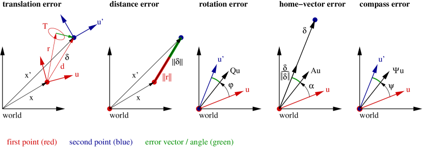
Figure 1: Cost functions. Each diagram shows the computation of the cost term for a pair of poses in the plane (red and blue dots and orientation vectors). Green distances and green angles visualize errors. The uncertainty is only visualized for the translation error (error ellipse); for the other cost functions, the one-dimensional translatory and angular uncertainties are not shown.

4.2 Cost Functions and Constraint

An issue to address in the design of the cost functions is how they are affected by the unit-length constraint on the orientation vectors they are depending on. The weakest requirement is that the cost functions show the desired effect at least if the constraint is fulfilled. This may allow for negative costs which is at least unusual and could possibly lead to problems in the Lagrange-Newton descent (e.g. getting stuck in compromise solutions). An intermediate requirement is therefore that the cost functions are in addition non-negative. The strongest requirement is that the cost functions are both non-negative and invariant of constraint violations. The complexity of cost functions and their derivatives grows with the strength of the requirement.

The question is whether and how the three requirement levels affect the performance of Lagrange-Newton SAM. Below we explore the alternatives for all rotational cost functions by defining three different variants bundled in two forms. This concerns the rotation error (odometry) and the home-vector and compass error (homing). The translation error (odometry) fulfills the intermediate requirement, but no version with the strongest requirement has been explored yet. The distance error (odometry) does not include orientation vectors and is therefore not affected.

4.3 Generic Rotational Cost Function

Below we define two purely rotational cost functions (rotation error and compass error) which only depend on $\mathbf{u}$ and $\mathbf{u}^{\prime}$. Both have the same form and can therefore be treated in the same way. (Note that the home-vector error is also a rotational cost function, but has a special form and will therefore be treated separately.) Let $\boldsymbol{\Phi}$ be an orthogonal orientation matrix (corresponding to an angle $\varphi$). We explore three alternative variants of rotational cost functions:

$$s\left(\boldsymbol{\Phi},\mathbf{p},\mathbf{p}^{\prime}\right) =1-\left(\boldsymbol{\Phi}\mathbf{u}\right)^{T}\mathbf{u}^{\prime}$$ (26)

$$s\left(\boldsymbol{\Phi},\mathbf{p},\mathbf{p}^{\prime}\right) =\left\|\mathbf{u}\right\|\left\|\mathbf{u}^{\prime}\right\|-\left(\boldsymbol{\Phi}\mathbf{u}\right)^{T}\mathbf{u}^{\prime}$$ (27)

$$\bar{s}\left(\boldsymbol{\Phi},\mathbf{p},\mathbf{p}^{\prime}\right) =1-\left(\boldsymbol{\Phi}{\,\frac{\mathbf{u}}{\left\|\mathbf{u}\right\|}\,}\right)^{T}{\,\frac{\mathbf{u}^{\prime}}{\left\|\mathbf{u}^{\prime}\right\|}\,}.$$ (28)

The term $\boldsymbol{\Phi}\mathbf{u}$ expresses a rotation of the first orientation vector $\mathbf{u}$ by the angle $\varphi$ expressed by the orthogonal orientation matrix $\boldsymbol{\Phi}$. The rotated orientation vector $\boldsymbol{\Phi}\mathbf{u}$ is matched to the second orientation vector $\mathbf{u}^{\prime}$. (In the third variant, $\mathbf{u}$ and $\mathbf{u}^{\prime}$ are normalized.) The generic rotational cost functions do not include uncertainty terms; these are introduced later for the specific cost functions.

In the first variant above (weakest requirement, see above), we determine a scalar product between $\boldsymbol{\Phi}\mathbf{u}$ and $\mathbf{u}^{\prime}$ and subtract it from $1$ to obtain a distance measure. If $\mathbf{u}$ and $\mathbf{u}^{\prime}$ are unit vectors, the last factor corresponds to $1-\cos\beta$ where $\beta$ is the angle between $\boldsymbol{\Phi}\mathbf{u}$ and $\mathbf{u}^{\prime}$. The Taylor expansion of $\cos\beta$ for small $\beta$ gives $\cos\beta\approx 1-\frac{1}{2}\beta^{2}$, so for small $\beta$ we have a quadratic error as for the translation error (see below). If $\mathbf{u}$ or $\mathbf{u}^{\prime}$ deviate from unit length, the costs can become negative in the first variant.

To avoid negative costs while keeping the cost function simple, we introduced the second variant (intermediate requirement) which differs in the first summand. Non-negativity is ensured by exploiting the Cauchy-Schwarz inequality (note that $\boldsymbol{\Phi}$ is orthogonal and the norm is invariant to multiplication by an orthogonal matrix). This variant is still affected by constraint violations.

The third variant normalizes the orientation vectors $\mathbf{u}$ and $\mathbf{u}^{\prime}$ to unit length such that the costs are always non-negative and the cost function is invariant of constraint violations (strongest requirement).

The first two variants are similar, so we fuse them using configuration parameters $t_{1}$ and $\bar{t}_{1}=1-t_{1}$ with $t_{1}\in\{0,1\}$:

$$s\left(\boldsymbol{\Phi},\mathbf{p},\mathbf{p}^{\prime}\right) =t_{1}+\bar{t}_{1}\left\|\mathbf{u}\right\|\left\|\mathbf{u}^{\prime}\right\|-\left(\boldsymbol{\Phi}\mathbf{u}\right)^{T}\mathbf{u}^{\prime}.$$ (29)

This form is later referred to as “first form”, while equation (28) is referred to as “second form”.

In all rotational cost functions introduced below, the same factor $\gamma$ is used as a weight factor (while translatory cost functions implicitly have unit weight). Even though rotatory and translatory cost functions are similar for small deviations, rotational cost terms are still different in character from translatory terms for larger deviations, as they are restricted in range (at least on the constraint) and cyclic.

4.4 Odometry Measurement

The odometry measurement between the first and second robot pose is described by vector $\mathbf{r}$ (in robot coordinates of the first robot pose) and orientation change vector $\mathbf{q}$ (or the corresponding orientation matrix $\mathbf{Q}$).

The uncertainty of the pose is described by the covariance matrix $\mathbf{C}$ (in robot coordinates of the first pose):

$$\mathbf{C} =\begin{pmatrix}\mathbf{T}&\mathbf{b}\\ \mathbf{b}^{T}&\sigma^{2}\end{pmatrix}$$ (30)

We ignore the cross-covariance terms $\mathbf{b}$ and $\mathbf{b}^{T}$ and approximate

$$\mathbf{C} \approx\begin{pmatrix}\mathbf{T}&\mathbf{0}_{2}\\ \mathbf{0}_{2}^{T}&\sigma^{2}\end{pmatrix}.$$ (31)

Here, the covariance matrix $\mathbf{T}$ describes the translatory uncertainty, the standard deviation $\sigma$ the angular uncertainty. In the following, we treat the translation error and the rotation error separately. In addition, we define a distance error which depends on the difference in measured and estimated distance between first and second position.

4.4.1 Translation Error

The translation error is defined as a Mahalanobis distance:

$$f\left(\mathbf{p},\mathbf{p}^{\prime}\right) =\frac{1}{2}\,\left(\mathbf{d}-\mathbf{r}\right)^{T}\mathbf{T}^{-1}\left(\mathbf{d}-\mathbf{r}\right)$$ (32)

where $\mathbf{d}=\mathbf{d}\left(\mathbf{x},\mathbf{u},\mathbf{x}^{\prime}\right)$ is the estimated position change in robot coordinates of the first pose, obtained from the estimated position change in world coordinates $\boldsymbol{\delta}=\mathbf{x}^{\prime}-\mathbf{x}$:

$$\mathbf{d} =\mathbf{U}^{T}\boldsymbol{\delta}=\mathbf{U}^{T}\left(\mathbf{x}^{\prime}-\mathbf{x}\right)=\begin{pmatrix}u_{1}&-u_{2}\\ u_{2}&u_{1}\end{pmatrix}^{T}\left(\mathbf{x}^{\prime}-\mathbf{x}\right).$$ (33)

4.4.2 Distance Error

The distance error is defined with measured distance $\varrho=\left\|\mathbf{r}\right\|$ and estimated distance $\left\|\boldsymbol{\delta}\right\|$ as:

$$e\left(\mathbf{p},\mathbf{p}^{\prime}\right) =\frac{1}{2}\,{\,\frac{1}{\sigma_{e}}\,}\left(\left\|\mathbf{x}^{\prime}-\mathbf{x}\right\|-\varrho\right)^{2}=\frac{1}{2}\,{\,\frac{1}{\sigma_{e}}\,}\left(\left\|\boldsymbol{\delta}\right\|-\varrho\right)^{2}.$$ (34)

The distance error is introduced as a second example of a translatory cost function and for tests of the implementation, but is not used in the experiments described below.

4.4.3 Rotation Error

The rotation error is defined in two forms by

$$g\left(\mathbf{p},\mathbf{p}^{\prime}\right) =\gamma{\,\frac{1}{\sigma^{2}}\,}s\left(\mathbf{Q},\mathbf{p},\mathbf{p}^{\prime}\right)=\gamma{\,\frac{1}{\sigma^{2}}\,}\left(t_{1}+\bar{t}_{1}\left\|\mathbf{u}\right\|\left\|\mathbf{u}^{\prime}\right\|-\left[\mathbf{Q}\mathbf{u}\right]^{T}\mathbf{u}^{\prime}\right)$$ (35)

$$\bar{g}\left(\mathbf{p},\mathbf{p}^{\prime}\right) =\gamma{\,\frac{1}{\sigma^{2}}\,}\bar{s}\left(\mathbf{Q},\mathbf{p},\mathbf{p}^{\prime}\right)=\gamma{\,\frac{1}{\sigma^{2}}\,}\left(1-\left[\mathbf{Q}{\,\frac{\mathbf{u}}{\left\|\mathbf{u}\right\|}\,}\right]^{T}{\,\frac{\mathbf{u}^{\prime}}{\left\|\mathbf{u}^{\prime}\right\|}\,}\right).$$ (36)

It depends on the cosine of the angle between the orientation vector of the first pose, rotated by the odometry rotation measurement (robot coordinates), and the orientation vector of the second pose.

4.5 Homing Measurement

We assume that a homing measurement delivers two orientation vectors with unit length: $\boldsymbol{\alpha}$ (or the corresponding orientation matrix $\boldsymbol{A}$) points approximately from the first to the second pose (in robot coordinates of the first pose), and $\boldsymbol{\psi}$ (or the corresponding orientation matrix $\boldsymbol{\Psi}$) is a measurement of the orientation difference between the second and the first pose.

The uncertainty of these two measurements is described by the standard deviations $\sigma_{h}$ (home vector) and $\sigma_{c}$ (compass).

4.5.1 Home-Vector Error

The home-vector error is defined in two forms by

$$h\left(\mathbf{p},\mathbf{p}^{\prime}\right) =\gamma{\,\frac{1}{\sigma_{h}^{2}}\,}\left(t_{1}+\bar{t}_{1}\left\|\mathbf{u}\right\|-\left[\boldsymbol{A}\mathbf{u}\right]^{T}{\,\frac{\boldsymbol{\delta}}{\left\|\boldsymbol{\delta}\right\|}\,}\right)$$ (37)

$$\bar{h}\left(\mathbf{p},\mathbf{p}^{\prime}\right) =\gamma{\,\frac{1}{\sigma_{h}^{2}}\,}\left(1-\left[\boldsymbol{A}{\,\frac{\mathbf{u}}{\left\|\mathbf{u}\right\|}\,}\right]^{T}{\,\frac{\boldsymbol{\delta}}{\left\|\boldsymbol{\delta}\right\|}\,}\right).$$ (38)

It depends on the cosine of the angle between the orientation vector of the first pose, rotated by the home-vector angle measurement (robot coordinates), and the unit vector pointing from the first to the second pose. Note that this is a rotational measure (as the rotation error above and the compass error below), but the second orientation vector is determined from the normalized home vector and not from the orientation vector of a pose.

4.5.2 Compass Error

The compass error is defined in two forms by

$$c\left(\mathbf{p},\mathbf{p}^{\prime}\right) =\gamma{\,\frac{1}{\sigma_{c}^{2}}\,}s\left(\boldsymbol{\Psi},\mathbf{p},\mathbf{p}^{\prime}\right)=\gamma{\,\frac{1}{\sigma_{c}^{2}}\,}\left(t_{1}+\bar{t}_{1}\left\|\mathbf{u}\right\|\left\|\mathbf{u}^{\prime}\right\|-\left[\boldsymbol{\Psi}\mathbf{u}\right]^{T}\mathbf{u}^{\prime}\right)$$ (39)

$$\bar{c}\left(\mathbf{p},\mathbf{p}^{\prime}\right) =\gamma{\,\frac{1}{\sigma_{c}^{2}}\,}\bar{s}\left(\boldsymbol{\Psi},\mathbf{p},\mathbf{p}^{\prime}\right)=\gamma{\,\frac{1}{\sigma_{c}^{2}}\,}\left(1-\left[\boldsymbol{\Psi}{\,\frac{\mathbf{u}}{\left\|\mathbf{u}\right\|}\,}\right]^{T}{\,\frac{\mathbf{u}^{\prime}}{\left\|\mathbf{u}^{\prime}\right\|}\,}\right).$$ (40)

It depends on the cosine of the angle between the orientation vector of the first pose, rotated by the compass measurement (robot coordinates), and the orientation vector of the second pose.

5 Derivatives

In the following, we compute the first and second derivatives of all cost functions. Zero derivatives are omitted. For some steps, we used the Matrix Calculus tool at www.matrixcalculus.org (Laue et al., 2018, 2020), particularly the following derivatives

$$\frac{\partial}{\partial\mathbf{x}}\,\left\|\mathbf{x}\right\| ={\,\frac{\mathbf{x}^{T}}{\left\|\mathbf{x}\right\|}\,}=\mathbf{x}_{0}^{T}$$ (41)

$$\frac{\partial}{\partial\mathbf{x}}\,{\,\frac{\mathbf{x}}{\left\|\mathbf{x}\right\|}\,} ={\,\frac{\mathbf{I}_{2}}{\left\|\mathbf{x}\right\|}\,}-{\,\frac{\mathbf{x}\mathbf{x}^{T}}{\left\|\mathbf{x}\right\|^{3}}\,}={\,\frac{1}{\left\|\mathbf{x}\right\|}\,}\left(\mathbf{I}_{2}-\mathbf{x}_{0}\mathbf{x}_{0}^{T}\right)$$ (42)

$$\frac{\partial}{\partial\mathbf{x}}\,\left(\left\|\mathbf{x}\right\|\mathbf{v}\right) ={\,\frac{\mathbf{v}\mathbf{x}^{T}}{\left\|\mathbf{x}\right\|}\,}=\mathbf{v}\mathbf{x}_{0}^{T}$$ (43)

$$\frac{\partial}{\partial\mathbf{x}}\,{\,\frac{\mathbf{v}}{\left\|\mathbf{x}\right\|}\,} =-{\,\frac{\mathbf{v}\mathbf{x}^{T}}{\left\|\mathbf{x}\right\|^{3}}\,}=-{\,\frac{\mathbf{v}\mathbf{x}_{0}^{T}}{\left\|\mathbf{x}\right\|^{2}}\,}$$ (44)

 

$$\phantom{{}={}}\frac{\partial}{\partial\mathbf{x}}\,{\,\frac{\mathbf{x}\mathbf{x}^{T}\mathbf{v}}{\left\|\mathbf{x}\right\|^{3}}\,}$$

$$={\,\frac{\left(\mathbf{x}^{T}\mathbf{v}\right)\mathbf{I}_{2}}{\left\|\mathbf{x}\right\|^{3}}\,}-3{\,\frac{\left(\mathbf{x}^{T}\mathbf{v}\right)\mathbf{x}\mathbf{x}^{T}}{\left\|\mathbf{x}\right\|^{5}}\,}+{\,\frac{\mathbf{x}\mathbf{v}^{T}}{\left\|\mathbf{x}\right\|^{3}}\,}$$ (45)

$$={\,\frac{1}{\left\|\mathbf{x}\right\|^{2}}\,}\left(\left[\mathbf{x}_{0}^{T}\mathbf{v}\right]\mathbf{I}_{2}-3\left[\mathbf{x}_{0}^{T}\mathbf{v}\right]\mathbf{x}_{0}\mathbf{x}_{0}^{T}+\mathbf{x}_{0}\mathbf{v}^{T}\right)$$ (46)

$$={\,\frac{1}{\left\|\mathbf{x}\right\|^{2}}\,}\left(\left[\mathbf{x}_{0}^{T}\mathbf{v}\right]\left[\mathbf{I}_{2}-3\mathbf{x}_{0}\mathbf{x}_{0}^{T}\right]+\mathbf{x}_{0}\mathbf{v}^{T}\right)$$ (47)

 

$$\phantom{{}={}}\frac{\partial}{\partial\mathbf{x}}\,\left(\left[{\,\frac{\mathbf{I}_{2}}{\left\|\mathbf{x}\right\|}\,}-{\,\frac{\mathbf{x}\mathbf{x}^{T}}{\left\|\mathbf{x}\right\|^{3}}\,}\right]\mathbf{v}\right)$$

$$=-{\,\frac{1}{\left\|\mathbf{x}\right\|^{2}}\,}\left({\,\frac{\mathbf{v}\mathbf{x}^{T}}{\left\|\mathbf{x}\right\|}\,}+{\,\frac{\left[\mathbf{x}^{T}\mathbf{v}\right]\mathbf{I}_{2}}{\left\|\mathbf{x}\right\|}\,}-{\,\frac{3\left[\mathbf{x}^{T}\mathbf{v}\right]\mathbf{x}\mathbf{x}^{T}}{\left\|\mathbf{x}\right\|^{3}}\,}+{\,\frac{\mathbf{x}\mathbf{v}^{T}}{\left\|\mathbf{x}\right\|}\,}\right)$$ (48)

$$=-{\,\frac{1}{\left\|\mathbf{x}\right\|^{2}}\,}\left(\mathbf{v}\mathbf{x}_{0}^{T}+\left[\mathbf{x}_{0}^{T}\mathbf{v}\right]\mathbf{I}_{2}-3\left[\mathbf{x}_{0}^{T}\mathbf{v}\right]\mathbf{x}_{0}\mathbf{x}_{0}^{T}+\mathbf{x}_{0}\mathbf{v}^{T}\right)$$ (49)

$$=-{\,\frac{1}{\left\|\mathbf{x}\right\|^{2}}\,}\left(\mathbf{v}\mathbf{x}_{0}^{T}+\left[\mathbf{x}_{0}^{T}\mathbf{v}\right]\left[\mathbf{I}_{2}-3\mathbf{x}_{0}\mathbf{x}_{0}^{T}\right]+\mathbf{x}_{0}\mathbf{v}^{T}\right)$$ (50)

where

$$\mathbf{x}_{0} ={\,\frac{\mathbf{x}}{\left\|\mathbf{x}\right\|}\,}.$$ (51)

5.1 First Derivatives

In the following, we apply the chain rule in vector form (see e.g. Deisenroth et al., 2020, p.129). Dimensions are $n$: $1\leq n$; $m$: $1\leq m$, variables and functions are $\mathbf{x}$: arbitrary, $n\times 1$; $\mathbf{z}$: arbitrary, $m\times 1$; $\mathbf{f}$: arbitrary, $m\times 1$; $g$: scalar, $1\times 1$; $y$: scalar, $1\times 1$:

$$\mathbf{z} =\mathbf{f}\left(\mathbf{x}\right)$$ (52)

$$y =g\left(\mathbf{z}\right)$$ (53)

$$\frac{\partial}{\partial\mathbf{x}}\,g =\left(\frac{\partial}{\partial\mathbf{z}}\,g\right)\left(\frac{\partial}{\partial\mathbf{x}}\,\mathbf{f}\right).$$ (54)

Note that the first factor (a gradient) is a row vector, and the second factor is a Jacobian matrix; their product is a row vector. The chain rule can also be applied for multi-step dependencies between vectors, e.g. in

$$\frac{\partial}{\partial\mathbf{x}}\,h\left(\mathbf{p},\mathbf{p}^{T}\right) =\left(\frac{\partial}{\partial\boldsymbol{\delta}}\,h\left(\mathbf{p},\mathbf{p}^{T}\right)\right)\left(\frac{\partial}{\partial\mathbf{x}}\,\boldsymbol{\delta}\right)=\left(\frac{\partial}{\partial\boldsymbol{\delta}_{0}}\,h\left(\mathbf{p},\mathbf{p}^{T}\right)\right)\left(\frac{\partial}{\partial\boldsymbol{\delta}}\,\boldsymbol{\delta}_{0}\right)\left(\frac{\partial}{\partial\mathbf{x}}\,\boldsymbol{\delta}\right).$$ (55)

5.2 First Derivatives of Generic Rotational Cost Function

We define

$$\mathbf{u}_{0} ={\,\frac{\mathbf{u}}{\left\|\mathbf{u}\right\|}\,}$$ (56)

$${{}{\mathbf{u}^{\prime}_{0}}} ={\,\frac{\mathbf{u}^{\prime}}{\left\|\mathbf{u}^{\prime}\right\|}\,}$$ (57)

and get for the first form

$$\phantom{{}={}}\frac{\partial}{\partial\mathbf{u}}\,s\left(\boldsymbol{\Phi},\mathbf{p},\mathbf{p}^{\prime}\right)$$

$$=\frac{\partial}{\partial\mathbf{u}}\,\left(t_{1}+\bar{t}_{1}\left\|\mathbf{u}\right\|\left\|\mathbf{u}^{\prime}\right\|-\left[\boldsymbol{\Phi}\mathbf{u}\right]^{T}\mathbf{u}^{\prime}\right)$$ (58)

$$=\frac{\partial}{\partial\mathbf{u}}\,\left(t_{1}+\bar{t}_{1}\left\|\mathbf{u}\right\|\left\|\mathbf{u}^{\prime}\right\|-\mathbf{u}^{\prime T}\boldsymbol{\Phi}\mathbf{u}\right)$$ (59)

$$=\bar{t}_{1}\left\|\mathbf{u}^{\prime}\right\|{\,\frac{\mathbf{u}^{T}}{\left\|\mathbf{u}\right\|}\,}-\mathbf{u}^{\prime T}\boldsymbol{\Phi}$$ (60)

$$=\bar{t}_{1}\left\|\mathbf{u}^{\prime}\right\|\mathbf{u}_{0}^{T}-\mathbf{u}^{\prime T}\boldsymbol{\Phi}$$ (61)

 

$$\phantom{{}={}}\frac{\partial}{\partial\mathbf{u}^{\prime}}\,s\left(\boldsymbol{\Phi},\mathbf{p},\mathbf{p}^{\prime}\right)$$

$$=\frac{\partial}{\partial\mathbf{u}^{\prime}}\,\left(t_{1}+\bar{t}_{1}\left\|\mathbf{u}\right\|\left\|\mathbf{u}^{\prime}\right\|-\left[\boldsymbol{\Phi}\mathbf{u}\right]^{T}\mathbf{u}^{\prime}\right)$$ (62)

$$=\frac{\partial}{\partial\mathbf{u}^{\prime}}\,\left(t_{1}+\bar{t}_{1}\left\|\mathbf{u}\right\|\left\|\mathbf{u}^{\prime}\right\|-\mathbf{u}^{T}\boldsymbol{\Phi}^{T}\mathbf{u}^{\prime}\right)$$ (63)

$$=\bar{t}_{1}\left\|\mathbf{u}\right\|{\,\frac{\mathbf{u}^{\prime T}}{\left\|\mathbf{u}^{\prime}\right\|}\,}-\mathbf{u}^{T}\boldsymbol{\Phi}^{T}$$ (64)

$$=\bar{t}_{1}\left\|\mathbf{u}\right\|{{}{\mathbf{u}^{\prime}_{0}}}^{T}-\mathbf{u}^{T}\boldsymbol{\Phi}^{T}.$$ (65)

For the second form, we get

$$\phantom{{}={}}\frac{\partial}{\partial\mathbf{u}}\,\bar{s}\left(\boldsymbol{\Phi},\mathbf{p},\mathbf{p}^{\prime}\right)$$

$$=\frac{\partial}{\partial\mathbf{u}}\,\left(1-\left[\boldsymbol{\Phi}{\,\frac{\mathbf{u}}{\left\|\mathbf{u}\right\|}\,}\right]^{T}{\,\frac{\mathbf{u}^{\prime}}{\left\|\mathbf{u}^{\prime}\right\|}\,}\right)$$ (66)

$$=\frac{\partial}{\partial\mathbf{u}}\,\left(1-{\,\frac{\mathbf{u}^{\prime T}}{\left\|\mathbf{u}^{\prime}\right\|}\,}\boldsymbol{\Phi}{\,\frac{\mathbf{u}}{\left\|\mathbf{u}\right\|}\,}\right)$$ (67)

$$=-{\,\frac{\mathbf{u}^{\prime T}}{\left\|\mathbf{u}^{\prime}\right\|}\,}\boldsymbol{\Phi}\left({\,\frac{\mathbf{I}_{2}}{\left\|\mathbf{u}\right\|}\,}-{\,\frac{\mathbf{u}\mathbf{u}^{T}}{\left\|\mathbf{u}\right\|^{3}}\,}\right)$$ (68)

$$=-{{}{\mathbf{u}^{\prime}_{0}}}^{T}\boldsymbol{\Phi}{\,\frac{1}{\left\|\mathbf{u}\right\|}\,}\left(\mathbf{I}_{2}-\mathbf{u}_{0}\mathbf{u}_{0}^{T}\right)$$ (69)

 

$$\phantom{{}={}}\frac{\partial}{\partial\mathbf{u}^{\prime}}\,\bar{s}\left(\boldsymbol{\Phi},\mathbf{p},\mathbf{p}^{\prime}\right)$$

$$=\frac{\partial}{\partial\mathbf{u}^{\prime}}\,\left(1-\left[\boldsymbol{\Phi}{\,\frac{\mathbf{u}}{\left\|\mathbf{u}\right\|}\,}\right]^{T}{\,\frac{\mathbf{u}^{\prime}}{\left\|\mathbf{u}^{\prime}\right\|}\,}\right)$$ (70)

$$=\frac{\partial}{\partial\mathbf{u}^{\prime}}\,\left(1-{\,\frac{\mathbf{u}^{T}}{\left\|\mathbf{u}\right\|}\,}\boldsymbol{\Phi}^{T}{\,\frac{\mathbf{u}^{\prime}}{\left\|\mathbf{u}^{\prime}\right\|}\,}\right)$$ (71)

$$=-{\,\frac{\mathbf{u}^{T}}{\left\|\mathbf{u}\right\|}\,}\boldsymbol{\Phi}^{T}\left({\,\frac{\mathbf{I}_{2}}{\left\|\mathbf{u}^{\prime}\right\|}\,}-{\,\frac{\mathbf{u}^{\prime}\mathbf{u}^{\prime T}}{\left\|\mathbf{u}^{\prime}\right\|^{3}}\,}\right)$$ (72)

$$=-\mathbf{u}_{0}^{T}\boldsymbol{\Phi}^{T}{\,\frac{1}{\left\|\mathbf{u}^{\prime}\right\|}\,}\left(\mathbf{I}_{2}-{{}{\mathbf{u}^{\prime}_{0}}}{{}{\mathbf{u}^{\prime}_{0}}}^{T}\right).$$ (73)

5.3 First Derivatives of Translation Error

We compute the first derivatives of the translation error (32):

$$\phantom{{}={}}\frac{\partial}{\partial\mathbf{x}}\,f\left(\mathbf{p},\mathbf{p}^{\prime}\right)$$

$$=\left(\frac{\partial}{\partial\mathbf{d}}\,f\left(\mathbf{p},\mathbf{p}^{\prime}\right)\right)\left(\frac{\partial}{\partial\mathbf{x}}\,\mathbf{d}\left(\mathbf{x},\mathbf{u},\mathbf{x}^{\prime}\right)\right)$$ (74)

$$=\left(\mathbf{d}\left(\mathbf{x},\mathbf{u},\mathbf{x}^{\prime}\right)-\mathbf{r}\right)^{T}\mathbf{T}^{-1}\left(\frac{\partial}{\partial\mathbf{x}}\,\left[\mathbf{U}^{T}\left\{\mathbf{x}^{\prime}-\mathbf{x}\right\}\right]\right)$$ (75)

$$=-\left(\mathbf{d}\left(\mathbf{x},\mathbf{u},\mathbf{x}^{\prime}\right)-\mathbf{r}\right)^{T}\mathbf{T}^{-1}\mathbf{U}^{T}$$ (76)

 

$$\phantom{{}={}}\frac{\partial}{\partial\mathbf{x}^{\prime}}\,f\left(\mathbf{p},\mathbf{p}^{\prime}\right)$$

$$=\left(\frac{\partial}{\partial\mathbf{d}}\,f\left(\mathbf{p},\mathbf{p}^{\prime}\right)\right)\left(\frac{\partial}{\partial\mathbf{x}^{\prime}}\,\mathbf{d}\left(\mathbf{x},\mathbf{u},\mathbf{x}^{\prime}\right)\right)$$ (77)

$$=\left(\mathbf{d}\left(\mathbf{x},\mathbf{u},\mathbf{x}^{\prime}\right)-\mathbf{r}\right)^{T}\mathbf{T}^{-1}\left(\frac{\partial}{\partial\mathbf{x}^{\prime}}\,\left[\mathbf{U}^{T}\left\{\mathbf{x}^{\prime}-\mathbf{x}\right\}\right]\right)$$ (78)

$$=\left(\mathbf{d}\left(\mathbf{x},\mathbf{u},\mathbf{x}^{\prime}\right)-\mathbf{r}\right)^{T}\mathbf{T}^{-1}\mathbf{U}^{T}.$$ (79)

 

With the following intermediate result (see also equation (18))

$$\phantom{{}={}}\frac{\partial}{\partial\mathbf{u}}\,\mathbf{d}\left(\mathbf{x},\mathbf{u},\mathbf{x}^{\prime}\right)$$

$$=\frac{\partial}{\partial\mathbf{u}}\,\left(\mathbf{U}^{T}\boldsymbol{\delta}\right)$$ (80)

$$=\frac{\partial}{\partial\mathbf{u}}\,\left(\begin{pmatrix}u_{1}&-u_{2}\\ u_{2}&u_{1}\end{pmatrix}^{T}\boldsymbol{\delta}\right)$$ (81)

$$=\frac{\partial}{\partial\mathbf{u}}\,\left(\begin{pmatrix}u_{1}&u_{2}\\ -u_{2}&u_{1}\end{pmatrix}\begin{pmatrix}\delta_{1}\\ \delta_{2}\end{pmatrix}\right)$$ (82)

$$=\frac{\partial}{\partial\mathbf{u}}\,\begin{pmatrix}u_{1}\delta_{1}+u_{2}\delta_{2}\\ \left(-u_{2}\delta_{1}\right)+u_{1}\delta_{2}\end{pmatrix}$$ (83)

$$=\begin{pmatrix}\delta_{1}&\delta_{2}\\ \delta_{2}&-\delta_{1}\end{pmatrix}$$ (84)

$$=\boldsymbol{\Delta}$$ (85)

$$=\overline{\boldsymbol{\Omega}}\left(\boldsymbol{\delta}\right)$$ (86)

we get

$$\phantom{{}={}}\frac{\partial}{\partial\mathbf{u}}\,f\left(\mathbf{p},\mathbf{p}^{\prime}\right)$$

$$=\left(\frac{\partial}{\partial\mathbf{d}}\,f\left(\mathbf{p},\mathbf{p}^{\prime}\right)\right)\left(\frac{\partial}{\partial\mathbf{u}}\,\mathbf{d}\left(\mathbf{x},\mathbf{u},\mathbf{x}^{\prime}\right)\right)$$ (87)

$$=\left(\mathbf{d}\left(\mathbf{x},\mathbf{u},\mathbf{x}^{\prime}\right)-\mathbf{r}\right)^{T}\mathbf{T}^{-1}\left(\frac{\partial}{\partial\mathbf{u}}\,\mathbf{d}\left(\mathbf{x},\mathbf{u},\mathbf{x}^{\prime}\right)\right)$$ (88)

$$=\left(\mathbf{d}\left(\mathbf{x},\mathbf{u},\mathbf{x}^{\prime}\right)-\mathbf{r}\right)^{T}\mathbf{T}^{-1}\boldsymbol{\Delta}$$ (89)

$$=\left(\mathbf{d}\left(\mathbf{x},\mathbf{u},\mathbf{x}^{\prime}\right)-\mathbf{r}\right)^{T}\mathbf{T}^{-1}\begin{pmatrix}\delta_{1}&\delta_{2}\\ \delta_{2}&-\delta_{1}\end{pmatrix}$$ (90)

$$=\left(\mathbf{d}\left(\mathbf{x},\mathbf{u},\mathbf{x}^{\prime}\right)-\mathbf{r}\right)^{T}\mathbf{T}^{-1}\begin{pmatrix}x^{\prime}_{1}-x_{1}&x^{\prime}_{2}-x_{2}\\ x^{\prime}_{2}-x_{2}&-\left(x^{\prime}_{1}-x_{1}\right)\end{pmatrix}.$$ (91)

5.4 First Derivatives of Distance Error

We use

$$\boldsymbol{\delta}_{0} ={\,\frac{\boldsymbol{\delta}}{\left\|\boldsymbol{\delta}\right\|}\,}$$ (92)

to compute the first derivatives of the distance error (34):

$$\phantom{{}={}}\frac{\partial}{\partial\mathbf{x}}\,e\left(\mathbf{p},\mathbf{p}^{\prime}\right)$$

$$=\left(\frac{\partial}{\partial\boldsymbol{\delta}}\,e\left(\mathbf{p},\mathbf{p}^{\prime}\right)\right)\left(\frac{\partial}{\partial\mathbf{x}}\,\boldsymbol{\delta}\right)$$ (93)

$$=\left(\frac{\partial}{\partial\boldsymbol{\delta}}\,\left[\frac{1}{2}\,{\,\frac{1}{\sigma_{e}}\,}\left\{\left\|\boldsymbol{\delta}\right\|-\varrho\right\}^{2}\right]\right)\left(-\mathbf{I}_{2}\right)$$ (94)

$$=-{\,\frac{1}{\sigma_{e}}\,}\left(\left\|\boldsymbol{\delta}\right\|-\varrho\right){\,\frac{\boldsymbol{\delta}^{T}}{\left\|\boldsymbol{\delta}\right\|}\,}$$ (95)

 

$$\phantom{{}={}}\frac{\partial}{\partial\mathbf{x}^{\prime}}\,e\left(\mathbf{p},\mathbf{p}^{\prime}\right)$$

$$=\left(\frac{\partial}{\partial\boldsymbol{\delta}}\,e\left(\mathbf{p},\mathbf{p}^{\prime}\right)\right)\left(\frac{\partial}{\partial\mathbf{x}^{\prime}}\,\boldsymbol{\delta}\right)$$ (96)

$$=\left(\frac{\partial}{\partial\boldsymbol{\delta}}\,\left[\frac{1}{2}\,{\,\frac{1}{\sigma_{e}}\,}\left\{\left\|\boldsymbol{\delta}\right\|-\varrho\right\}^{2}\right]\right)\mathbf{I}_{2}$$ (97)

$$={\,\frac{1}{\sigma_{e}}\,}\left(\left\|\boldsymbol{\delta}\right\|-\varrho\right){\,\frac{\boldsymbol{\delta}^{T}}{\left\|\boldsymbol{\delta}\right\|}\,}.$$ (98)

5.5 First Derivatives of Rotation Error

We get the first derivatives of the rotation error (35) and (36) from the generic solutions in section 5.2. For the first form we obtain

$$\phantom{{}={}}\frac{\partial}{\partial\mathbf{u}}\,g\left(\mathbf{p},\mathbf{p}^{\prime}\right)$$

$$=\gamma{\,\frac{1}{\sigma^{2}}\,}\left(\bar{t}_{1}\left\|\mathbf{u}^{\prime}\right\|\mathbf{u}_{0}^{T}-\mathbf{u}^{\prime T}\mathbf{Q}\right)$$ (99)

 

$$\phantom{{}={}}\frac{\partial}{\partial\mathbf{u}^{\prime}}\,g\left(\mathbf{p},\mathbf{p}^{\prime}\right)$$

$$=\gamma{\,\frac{1}{\sigma^{2}}\,}\left(\bar{t}_{1}\left\|\mathbf{u}\right\|{{}{\mathbf{u}^{\prime}_{0}}}^{T}-\mathbf{u}^{T}\mathbf{Q}^{T}\right).$$ (100)

For the second form we get

$$\phantom{{}={}}\frac{\partial}{\partial\mathbf{u}}\,\bar{g}\left(\mathbf{p},\mathbf{p}^{\prime}\right)$$

$$=-\gamma{\,\frac{1}{\sigma^{2}}\,}{{}{\mathbf{u}^{\prime}_{0}}}^{T}\mathbf{Q}{\,\frac{1}{\left\|\mathbf{u}\right\|}\,}\left(\mathbf{I}_{2}-\mathbf{u}_{0}\mathbf{u}_{0}^{T}\right)$$ (101)

 

$$\phantom{{}={}}\frac{\partial}{\partial\mathbf{u}^{\prime}}\,\bar{g}\left(\mathbf{p},\mathbf{p}^{\prime}\right)$$

$$=-\gamma{\,\frac{1}{\sigma^{2}}\,}\mathbf{u}_{0}^{T}\mathbf{Q}^{T}{\,\frac{1}{\left\|\mathbf{u}^{\prime}\right\|}\,}\left(\mathbf{I}_{2}-{{}{\mathbf{u}^{\prime}_{0}}}{{}{\mathbf{u}^{\prime}_{0}}}^{T}\right).$$ (102)

5.6 First Derivatives of Home-Vector Error

We compute the first derivatives of the home-vector error (37) and (38). We use

$$\boldsymbol{\delta}_{0} ={\,\frac{\boldsymbol{\delta}}{\left\|\boldsymbol{\delta}\right\|}\,}$$ (103)

$$\boldsymbol{\delta} =\mathbf{x}^{\prime}-\mathbf{x}$$ (104)

$$\frac{\partial}{\partial\mathbf{x}}\,\boldsymbol{\delta} =\frac{\partial}{\partial\mathbf{x}}\,\left(\mathbf{x}^{\prime}-\mathbf{x}\right)=-\mathbf{I}_{2}$$ (105)

$$\frac{\partial}{\partial\mathbf{x}^{\prime}}\,\boldsymbol{\delta} =\frac{\partial}{\partial\mathbf{x}^{\prime}}\,\left(\mathbf{x}^{\prime}-\mathbf{x}\right)=\mathbf{I}_{2}$$ (106)

and obtain for the first form

$$\phantom{{}={}}\frac{\partial}{\partial\mathbf{x}}\,h\left(\mathbf{p},\mathbf{p}^{\prime}\right)$$

$$=\left(\frac{\partial}{\partial\boldsymbol{\delta}_{0}}\,h\left(\mathbf{p},\mathbf{p}^{\prime}\right)\right)\left(\frac{\partial}{\partial\boldsymbol{\delta}}\,\boldsymbol{\delta}_{0}\right)\left(\frac{\partial}{\partial\mathbf{x}}\,\boldsymbol{\delta}\right)$$ (107)

$$=\left(\frac{\partial}{\partial\boldsymbol{\delta}_{0}}\,\left[\gamma{\,\frac{1}{\sigma_{h}^{2}}\,}\left\{t_{1}+\bar{t}_{1}\left\|\mathbf{u}\right\|-\left(\boldsymbol{A}\mathbf{u}\right)^{T}\boldsymbol{\delta}_{0}\right\}\right]\right)\left(\frac{\partial}{\partial\boldsymbol{\delta}}\,\boldsymbol{\delta}_{0}\right)\left(\frac{\partial}{\partial\mathbf{x}}\,\boldsymbol{\delta}\right)$$ (108)

$$=\gamma{\,\frac{1}{\sigma_{h}^{2}}\,}\mathbf{u}^{T}\boldsymbol{A}^{T}\left({\,\frac{\mathbf{I}_{2}}{\left\|\boldsymbol{\delta}\right\|}\,}-{\,\frac{\boldsymbol{\delta}\boldsymbol{\delta}^{T}}{\left\|\boldsymbol{\delta}\right\|^{3}}\,}\right)$$ (109)

$$=\gamma{\,\frac{1}{\sigma_{h}^{2}}\,}\mathbf{u}^{T}\boldsymbol{A}^{T}{\,\frac{1}{\left\|\boldsymbol{\delta}\right\|}\,}\left(\mathbf{I}_{2}-\boldsymbol{\delta}_{0}\boldsymbol{\delta}_{0}^{T}\right)$$ (110)

 

$$\phantom{{}={}}\frac{\partial}{\partial\mathbf{x}^{\prime}}\,h\left(\mathbf{p},\mathbf{p}^{\prime}\right)$$

$$=\left(\frac{\partial}{\partial\boldsymbol{\delta}_{0}}\,h\left(\mathbf{p},\mathbf{p}^{\prime}\right)\right)\left(\frac{\partial}{\partial\boldsymbol{\delta}}\,\boldsymbol{\delta}_{0}\right)\left(\frac{\partial}{\partial\mathbf{x}^{\prime}}\,\boldsymbol{\delta}\right)$$ (111)

$$=\left(\frac{\partial}{\partial\boldsymbol{\delta}_{0}}\,\left[\gamma{\,\frac{1}{\sigma_{h}^{2}}\,}\left\{t_{1}+\bar{t}_{1}\left\|\mathbf{u}\right\|-\left(\boldsymbol{A}\mathbf{u}\right)^{T}\boldsymbol{\delta}_{0}\right\}\right]\right)\left(\frac{\partial}{\partial\boldsymbol{\delta}}\,\boldsymbol{\delta}_{0}\right)\left(\frac{\partial}{\partial\mathbf{x}^{\prime}}\,\boldsymbol{\delta}\right)$$ (112)

$$=-\gamma{\,\frac{1}{\sigma_{h}^{2}}\,}\mathbf{u}^{T}\boldsymbol{A}^{T}\left({\,\frac{\mathbf{I}_{2}}{\left\|\boldsymbol{\delta}\right\|}\,}-{\,\frac{\boldsymbol{\delta}\boldsymbol{\delta}^{T}}{\left\|\boldsymbol{\delta}\right\|^{3}}\,}\right)$$ (113)

$$=-\gamma{\,\frac{1}{\sigma_{h}^{2}}\,}\mathbf{u}^{T}\boldsymbol{A}^{T}{\,\frac{1}{\left\|\boldsymbol{\delta}\right\|}\,}\left(\mathbf{I}_{2}-\boldsymbol{\delta}_{0}\boldsymbol{\delta}_{0}^{T}\right)$$ (114)

 

$$\phantom{{}={}}\frac{\partial}{\partial\mathbf{u}}\,h\left(\mathbf{p},\mathbf{p}^{\prime}\right)$$

$$=\frac{\partial}{\partial\mathbf{u}}\,\left(\gamma{\,\frac{1}{\sigma_{h}^{2}}\,}\left[t_{1}+\bar{t}_{1}\left\|\mathbf{u}\right\|-\left\{\boldsymbol{A}\mathbf{u}\right\}^{T}{\,\frac{\boldsymbol{\delta}}{\left\|\boldsymbol{\delta}\right\|}\,}\right]\right)$$ (115)

$$=\frac{\partial}{\partial\mathbf{u}}\,\left(\gamma{\,\frac{1}{\sigma_{h}^{2}}\,}\left[t_{1}+\bar{t}_{1}\left\|\mathbf{u}\right\|-{\,\frac{\boldsymbol{\delta}^{T}}{\left\|\boldsymbol{\delta}\right\|}\,}\boldsymbol{A}\mathbf{u}\right]\right)$$ (116)

$$=\gamma{\,\frac{1}{\sigma_{h}^{2}}\,}\left(\bar{t}_{1}{\,\frac{\mathbf{u}^{T}}{\left\|\mathbf{u}\right\|}\,}-{\,\frac{\boldsymbol{\delta}^{T}}{\left\|\boldsymbol{\delta}\right\|}\,}\boldsymbol{A}\right)$$ (117)

$$=\gamma{\,\frac{1}{\sigma_{h}^{2}}\,}\left(\bar{t}_{1}\mathbf{u}_{0}^{T}-\boldsymbol{\delta}_{0}^{T}\boldsymbol{A}\right).$$ (118)

For the second form we get

$$\phantom{{}={}}\frac{\partial}{\partial\mathbf{x}}\,\bar{h}\left(\mathbf{p},\mathbf{p}^{\prime}\right)$$

$$=\left(\frac{\partial}{\partial\boldsymbol{\delta}_{0}}\,\bar{h}\left(\mathbf{p},\mathbf{p}^{\prime}\right)\right)\left(\frac{\partial}{\partial\boldsymbol{\delta}}\,\boldsymbol{\delta}_{0}\right)\left(\frac{\partial}{\partial\mathbf{x}}\,\boldsymbol{\delta}\right)$$ (119)

$$=\left(\frac{\partial}{\partial\boldsymbol{\delta}_{0}}\,\left[\gamma{\,\frac{1}{\sigma_{h}^{2}}\,}\left\{1-\left(\boldsymbol{A}{\,\frac{\mathbf{u}}{\left\|\mathbf{u}\right\|}\,}\right)^{T}\boldsymbol{\delta}_{0}\right\}\right]\right)\left(\frac{\partial}{\partial\boldsymbol{\delta}}\,\boldsymbol{\delta}_{0}\right)\left(\frac{\partial}{\partial\mathbf{x}}\,\boldsymbol{\delta}\right)$$ (120)

$$=\gamma{\,\frac{1}{\sigma_{h}^{2}}\,}{\,\frac{\mathbf{u}^{T}}{\left\|\mathbf{u}\right\|}\,}\boldsymbol{A}^{T}\left({\,\frac{\mathbf{I}_{2}}{\left\|\boldsymbol{\delta}\right\|}\,}-{\,\frac{\boldsymbol{\delta}\boldsymbol{\delta}^{T}}{\left\|\boldsymbol{\delta}\right\|^{3}}\,}\right)$$ (121)

$$=\gamma{\,\frac{1}{\sigma_{h}^{2}}\,}\mathbf{u}_{0}^{T}\boldsymbol{A}^{T}{\,\frac{1}{\left\|\boldsymbol{\delta}\right\|}\,}\left(\mathbf{I}_{2}-\boldsymbol{\delta}_{0}\boldsymbol{\delta}_{0}^{T}\right)$$ (122)

 

$$\phantom{{}={}}\frac{\partial}{\partial\mathbf{x}^{\prime}}\,\bar{h}\left(\mathbf{p},\mathbf{p}^{\prime}\right)$$

$$=\left(\frac{\partial}{\partial\boldsymbol{\delta}_{0}}\,\bar{h}\left(\mathbf{p},\mathbf{p}^{\prime}\right)\right)\left(\frac{\partial}{\partial\boldsymbol{\delta}}\,\boldsymbol{\delta}_{0}\right)\left(\frac{\partial}{\partial\mathbf{x}^{\prime}}\,\boldsymbol{\delta}\right)$$ (123)

$$=\left(\frac{\partial}{\partial\boldsymbol{\delta}_{0}}\,\left[\gamma{\,\frac{1}{\sigma_{h}^{2}}\,}\left\{1-\left(\boldsymbol{A}{\,\frac{\mathbf{u}}{\left\|\mathbf{u}\right\|}\,}\right)^{T}\boldsymbol{\delta}_{0}\right\}\right]\right)\left(\frac{\partial}{\partial\boldsymbol{\delta}}\,\boldsymbol{\delta}_{0}\right)\left(\frac{\partial}{\partial\mathbf{x}^{\prime}}\,\boldsymbol{\delta}\right)$$ (124)

$$=-\gamma{\,\frac{1}{\sigma_{h}^{2}}\,}{\,\frac{\mathbf{u}^{T}}{\left\|\mathbf{u}\right\|}\,}\boldsymbol{A}^{T}\left({\,\frac{\mathbf{I}_{2}}{\left\|\boldsymbol{\delta}\right\|}\,}-{\,\frac{\boldsymbol{\delta}\boldsymbol{\delta}^{T}}{\left\|\boldsymbol{\delta}\right\|^{3}}\,}\right)$$ (125)

$$=-\gamma{\,\frac{1}{\sigma_{h}^{2}}\,}\mathbf{u}_{0}^{T}\boldsymbol{A}^{T}{\,\frac{1}{\left\|\boldsymbol{\delta}\right\|}\,}\left(\mathbf{I}_{2}-\boldsymbol{\delta}_{0}\boldsymbol{\delta}_{0}^{T}\right)$$ (126)

 

$$\phantom{{}={}}\frac{\partial}{\partial\mathbf{u}}\,\bar{h}\left(\mathbf{p},\mathbf{p}^{\prime}\right)$$

$$=\frac{\partial}{\partial\mathbf{u}}\,\left(\gamma{\,\frac{1}{\sigma_{h}^{2}}\,}\left[1-\left\{\boldsymbol{A}{\,\frac{\mathbf{u}}{\left\|\mathbf{u}\right\|}\,}\right\}^{T}{\,\frac{\boldsymbol{\delta}}{\left\|\boldsymbol{\delta}\right\|}\,}\right]\right)$$ (127)

$$=\frac{\partial}{\partial\mathbf{u}}\,\left(\gamma{\,\frac{1}{\sigma_{h}^{2}}\,}\left[1-{\,\frac{\boldsymbol{\delta}^{T}}{\left\|\boldsymbol{\delta}\right\|}\,}\boldsymbol{A}{\,\frac{\mathbf{u}}{\left\|\mathbf{u}\right\|}\,}\right]\right)$$ (128)

$$=-\gamma{\,\frac{1}{\sigma_{h}^{2}}\,}{\,\frac{\boldsymbol{\delta}^{T}}{\left\|\boldsymbol{\delta}\right\|}\,}\boldsymbol{A}\left({\,\frac{\mathbf{I}_{2}}{\left\|\mathbf{u}\right\|}\,}-{\,\frac{\mathbf{u}\mathbf{u}^{T}}{\left\|\mathbf{u}\right\|^{3}}\,}\right)$$ (129)

$$=-\gamma{\,\frac{1}{\sigma_{h}^{2}}\,}\boldsymbol{\delta}_{0}^{T}\boldsymbol{A}{\,\frac{1}{\left\|\mathbf{u}\right\|}\,}\left(\mathbf{I}_{2}-\mathbf{u}_{0}\mathbf{u}_{0}^{T}\right).$$ (130)

5.7 First Derivatives of Compass Error

We get the first derivatives of the compass error (39) and (40) from the generic solutions in section 5.2. For the first form we obtain

$$\phantom{{}={}}\frac{\partial}{\partial\mathbf{u}}\,c\left(\mathbf{p},\mathbf{p}^{\prime}\right)$$

$$=\gamma{\,\frac{1}{\sigma_{c}^{2}}\,}\left(\bar{t}_{1}\left\|\mathbf{u}^{\prime}\right\|\mathbf{u}_{0}^{T}-\mathbf{u}^{\prime T}\boldsymbol{\Psi}\right)$$ (131)

 

$$\phantom{{}={}}\frac{\partial}{\partial\mathbf{u}^{\prime}}\,c\left(\mathbf{p},\mathbf{p}^{\prime}\right)$$

$$=\gamma{\,\frac{1}{\sigma_{c}^{2}}\,}\left(\bar{t}_{1}\left\|\mathbf{u}\right\|{{}{\mathbf{u}^{\prime}_{0}}}^{T}-\mathbf{u}^{T}\boldsymbol{\Psi}^{T}\right).$$ (132)

For the second form we get

$$\phantom{{}={}}\frac{\partial}{\partial\mathbf{u}}\,\bar{c}\left(\mathbf{p},\mathbf{p}^{\prime}\right)$$

$$=-\gamma{\,\frac{1}{\sigma_{c}^{2}}\,}{{}{\mathbf{u}^{\prime}_{0}}}^{T}\boldsymbol{\Psi}{\,\frac{1}{\left\|\mathbf{u}\right\|}\,}\left(\mathbf{I}_{2}-\mathbf{u}_{0}\mathbf{u}_{0}^{T}\right)$$ (133)

 

$$\phantom{{}={}}\frac{\partial}{\partial\mathbf{u}^{\prime}}\,\bar{c}\left(\mathbf{p},\mathbf{p}^{\prime}\right)$$

$$=-\gamma{\,\frac{1}{\sigma_{c}^{2}}\,}\mathbf{u}_{0}^{T}\boldsymbol{\Psi}^{T}{\,\frac{1}{\left\|\mathbf{u}^{\prime}\right\|}\,}\left(\mathbf{I}_{2}-{{}{\mathbf{u}^{\prime}_{0}}}{{}{\mathbf{u}^{\prime}_{0}}}^{T}\right).$$ (134)

5.8 Second Derivatives

In the following, we exploit the fact that second derivatives w.r.t. the same (scalar) variables but in different order are identical, so we can reduce the number of derivatives to compute. When the final matrices are formed, the sub-blocks of the missing derivatives are the transposed sub-blocks of the ones which are specified.

Zero second derivatives are not listed.

Note that (second) derivatives of first derivatives with respect to the same vector variable are symmetric (which can be used to check the results).

For each cost function, we first determine the transposed of the first derivative (since the first derivatives are row vectors, but the partial derivative expects a column vector).

In intermediate steps, the orientation matrix $\mathbf{U}$ is expressed by $\mathbf{u}$ through $\mathbf{U}=\boldsymbol{\Omega}\left(\mathbf{u}\right)$ (see section 3). We also use

$$\boldsymbol{\Delta} =\overline{\boldsymbol{\Omega}}\left(\boldsymbol{\delta}\right)=\begin{pmatrix}\delta_{1}&\delta_{2}\\ \delta_{2}&-\delta_{1}\end{pmatrix}.$$ (135)

5.9 Second Derivatives of Generic Rotational Cost Function

For the first form we get

$$\phantom{{}={}}\frac{\partial}{\partial\mathbf{u}}\,\left(\frac{\partial}{\partial\mathbf{u}}\,s\left(\boldsymbol{\Phi},\mathbf{p},\mathbf{p}^{\prime}\right)\right)^{T}$$

$$=\frac{\partial}{\partial\mathbf{u}}\,\left(\bar{t}_{1}\left\|\mathbf{u}^{\prime}\right\|{\,\frac{\mathbf{u}}{\left\|\mathbf{u}\right\|}\,}-\boldsymbol{\Phi}^{T}\mathbf{u}^{\prime}\right)$$ (136)

$$=\bar{t}_{1}{\,\frac{\left\|\mathbf{u}^{\prime}\right\|}{\left\|\mathbf{u}\right\|}\,}\left(\mathbf{I}_{2}-\mathbf{u}_{0}\mathbf{u}_{0}^{T}\right)$$ (137)

 

$$\phantom{{}={}}\frac{\partial}{\partial\mathbf{u}^{\prime}}\,\left(\frac{\partial}{\partial\mathbf{u}}\,s\left(\boldsymbol{\Phi},\mathbf{p},\mathbf{p}^{\prime}\right)\right)^{T}$$

$$=\frac{\partial}{\partial\mathbf{u}^{\prime}}\,\left(\bar{t}_{1}\left\|\mathbf{u}^{\prime}\right\|{\,\frac{\mathbf{u}}{\left\|\mathbf{u}\right\|}\,}-\boldsymbol{\Phi}^{T}\mathbf{u}^{\prime}\right)$$ (138)

$$=\bar{t}_{1}{\,\frac{\mathbf{u}}{\left\|\mathbf{u}\right\|}\,}{\,\frac{\mathbf{u}^{\prime T}}{\left\|\mathbf{u}^{\prime}\right\|}\,}-\boldsymbol{\Phi}^{T}$$ (139)

$$=\bar{t}_{1}\mathbf{u}_{0}{{}{\mathbf{u}^{\prime}_{0}}}^{T}-\boldsymbol{\Phi}^{T}$$ (140)

 

$$\phantom{{}={}}\frac{\partial}{\partial\mathbf{u}^{\prime}}\,\left(\frac{\partial}{\partial\mathbf{u}^{\prime}}\,s\left(\boldsymbol{\Phi},\mathbf{p},\mathbf{p}^{\prime}\right)\right)^{T}$$

$$=\frac{\partial}{\partial\mathbf{u}^{\prime}}\,\left(\bar{t}_{1}\left\|\mathbf{u}\right\|{\,\frac{\mathbf{u}^{\prime}}{\left\|\mathbf{u}^{\prime}\right\|}\,}-\boldsymbol{\Phi}\mathbf{u}\right)$$ (141)

$$=\bar{t}_{1}{\,\frac{\left\|\mathbf{u}\right\|}{\left\|\mathbf{u}^{\prime}\right\|}\,}\left(\mathbf{I}_{2}-{{}{\mathbf{u}^{\prime}_{0}}}{{}{\mathbf{u}^{\prime}_{0}}}^{T}\right).$$ (142)

For the second form we get

$$\phantom{{}={}}\frac{\partial}{\partial\mathbf{u}}\,\left(\frac{\partial}{\partial\mathbf{u}}\,\bar{s}\left(\boldsymbol{\Phi},\mathbf{p},\mathbf{p}^{\prime}\right)\right)^{T}$$

$$=-\frac{\partial}{\partial\mathbf{u}}\,\left(\left[{\,\frac{\mathbf{I}_{2}}{\left\|\mathbf{u}\right\|}\,}-{\,\frac{\mathbf{u}\mathbf{u}^{T}}{\left\|\mathbf{u}\right\|^{3}}\,}\right]\boldsymbol{\Phi}^{T}{{}{\mathbf{u}^{\prime}_{0}}}\right)$$ (143)

$$={\,\frac{1}{\left\|\mathbf{u}\right\|^{2}}\,}\left(\boldsymbol{\Phi}^{T}{{}{\mathbf{u}^{\prime}_{0}}}\mathbf{u}_{0}^{T}+\left[\mathbf{u}_{0}^{T}\boldsymbol{\Phi}^{T}{{}{\mathbf{u}^{\prime}_{0}}}\right]\left[\mathbf{I}_{2}-3\mathbf{u}_{0}\mathbf{u}_{0}^{T}\right]+\mathbf{u}_{0}{{}{\mathbf{u}^{\prime}_{0}}}^{T}\boldsymbol{\Phi}\right)$$ (144)

 

$$\phantom{{}={}}\frac{\partial}{\partial\mathbf{u}^{\prime}}\,\left(\frac{\partial}{\partial\mathbf{u}}\,\bar{s}\left(\boldsymbol{\Phi},\mathbf{p},\mathbf{p}^{\prime}\right)\right)^{T}$$

$$=-\frac{\partial}{\partial\mathbf{u}^{\prime}}\,\left(\left[{\,\frac{\mathbf{I}_{2}}{\left\|\mathbf{u}\right\|}\,}-{\,\frac{\mathbf{u}\mathbf{u}^{T}}{\left\|\mathbf{u}\right\|^{3}}\,}\right]\boldsymbol{\Phi}^{T}{{}{\mathbf{u}^{\prime}_{0}}}\right)$$ (145)

$$=-\left({\,\frac{\mathbf{I}_{2}}{\left\|\mathbf{u}\right\|}\,}-{\,\frac{\mathbf{u}\mathbf{u}^{T}}{\left\|\mathbf{u}\right\|^{3}}\,}\right)\boldsymbol{\Phi}^{T}\left({\,\frac{\mathbf{I}_{2}}{\left\|\mathbf{u}^{\prime}\right\|}\,}-{\,\frac{\mathbf{u}^{\prime}\mathbf{u}^{\prime T}}{\left\|\mathbf{u}^{\prime}\right\|^{3}}\,}\right)$$ (146)

$$=-{\,\frac{1}{\left\|\mathbf{u}\right\|\left\|\mathbf{u}^{\prime}\right\|}\,}\left(\mathbf{I}_{2}-\mathbf{u}_{0}\mathbf{u}_{0}^{T}\right)\boldsymbol{\Phi}^{T}\left(\mathbf{I}_{2}-{{}{\mathbf{u}^{\prime}_{0}}}{{}{\mathbf{u}^{\prime}_{0}}}^{T}\right)$$ (147)

 

$$\phantom{{}={}}\frac{\partial}{\partial\mathbf{u}^{\prime}}\,\left(\frac{\partial}{\partial\mathbf{u}^{\prime}}\,\bar{s}\left(\boldsymbol{\Phi},\mathbf{p},\mathbf{p}^{\prime}\right)\right)^{T}$$

$$=-\frac{\partial}{\partial\mathbf{u}^{\prime}}\,\left(\left[{\,\frac{\mathbf{I}_{2}}{\left\|\mathbf{u}^{\prime}\right\|}\,}-{\,\frac{\mathbf{u}^{\prime}\mathbf{u}^{\prime T}}{\left\|\mathbf{u}^{\prime}\right\|^{3}}\,}\right]\boldsymbol{\Phi}\mathbf{u}_{0}\right)$$ (148)

$$={\,\frac{1}{\left\|\mathbf{u}^{\prime}\right\|^{2}}\,}\left(\boldsymbol{\Phi}\mathbf{u}_{0}{{}{\mathbf{u}^{\prime}_{0}}}^{T}+\left[{{}{\mathbf{u}^{\prime}_{0}}}^{T}\boldsymbol{\Phi}\mathbf{u}_{0}\right]\left[\mathbf{I}_{2}-3{{}{\mathbf{u}^{\prime}_{0}}}{{}{\mathbf{u}^{\prime}_{0}}}^{T}\right]+{{}{\mathbf{u}^{\prime}_{0}}}\mathbf{u}_{0}^{T}\boldsymbol{\Phi}^{T}\right).$$ (149)

5.10 Second Derivatives of Translation Error

For first derivative with respect to $\mathbf{x}$:

$$\phantom{{}={}}\left(\frac{\partial}{\partial\mathbf{x}}\,f\left(\mathbf{p},\mathbf{p}^{T}\right)\right)^{T}$$

$$=\left(-\left[\mathbf{d}\left(\mathbf{x},\mathbf{u},\mathbf{x}^{\prime}\right)-\mathbf{r}\right]^{T}\mathbf{T}^{-1}\mathbf{U}^{T}\right)^{T}$$ (150)

$$=-\mathbf{U}\mathbf{T}^{-1}\left(\mathbf{d}\left(\mathbf{x},\mathbf{u},\mathbf{x}^{\prime}\right)-\mathbf{r}\right)$$ (151)

$$=-\mathbf{U}\mathbf{T}^{-1}\left(\mathbf{U}^{T}\left[\mathbf{x}^{\prime}-\mathbf{x}\right]-\mathbf{r}\right).$$ (152)

Second derivatives:

$$\phantom{{}={}}\frac{\partial}{\partial\mathbf{x}}\,\left(\frac{\partial}{\partial\mathbf{x}}\,f\left(\mathbf{p},\mathbf{p}^{T}\right)\right)^{T}$$

$$=\frac{\partial}{\partial\mathbf{x}}\,\left(-\mathbf{U}\mathbf{T}^{-1}\left[\mathbf{U}^{T}\left\{\mathbf{x}^{\prime}-\mathbf{x}\right\}-\mathbf{r}\right]\right)$$ (153)

$$=\mathbf{U}\mathbf{T}^{-1}\mathbf{U}^{T}$$ (154)

 

$$\phantom{{}={}}\frac{\partial}{\partial\mathbf{x}^{\prime}}\,\left(\frac{\partial}{\partial\mathbf{x}}\,f\left(\mathbf{p},\mathbf{p}^{T}\right)\right)^{T}$$

$$=\frac{\partial}{\partial\mathbf{x}^{\prime}}\,\left(-\mathbf{U}\mathbf{T}^{-1}\left[\mathbf{U}^{T}\left\{\mathbf{x}^{\prime}-\mathbf{x}\right\}-\mathbf{r}\right]\right)$$ (155)

$$=-\mathbf{U}\mathbf{T}^{-1}\mathbf{U}^{T}$$ (156)

 

$$\phantom{{}={}}\frac{\partial}{\partial\mathbf{u}}\,\left(\frac{\partial}{\partial\mathbf{x}}\,f\left(\mathbf{p},\mathbf{p}^{T}\right)\right)^{T}$$

$$=\frac{\partial}{\partial\mathbf{u}}\,\left(-\mathbf{U}\mathbf{T}^{-1}\left[\mathbf{U}^{T}\boldsymbol{\delta}-\mathbf{r}\right]\right)$$ (157)

$$=-\frac{\partial}{\partial\mathbf{u}}\,\left(\mathbf{U}\mathbf{T}^{-1}\mathbf{U}^{T}\boldsymbol{\delta}-\mathbf{U}\mathbf{T}^{-1}\mathbf{r}\right)$$ (158)

$$=-\frac{\partial}{\partial\mathbf{u}}\,\left(\begin{pmatrix}\mathbf{u}^{T}\mathbf{M}\\ \mathbf{u}^{T}\mathbf{N}\end{pmatrix}\mathbf{T}^{-1}\begin{pmatrix}\mathbf{M}\mathbf{u}&\mathbf{N}\mathbf{u}\end{pmatrix}\boldsymbol{\delta}-\begin{pmatrix}\mathbf{u}^{T}\mathbf{M}\\ \mathbf{u}^{T}\mathbf{N}\end{pmatrix}\mathbf{T}^{-1}\mathbf{r}\right)$$ (159)

$$=-\frac{\partial}{\partial\mathbf{u}}\,\left(\begin{pmatrix}\mathbf{u}^{T}\mathbf{M}\mathbf{T}^{-1}\\ \mathbf{u}^{T}\mathbf{N}\mathbf{T}^{-1}\end{pmatrix}\begin{pmatrix}\mathbf{M}\mathbf{u}&\mathbf{N}\mathbf{u}\end{pmatrix}\boldsymbol{\delta}-\begin{pmatrix}\mathbf{u}^{T}\mathbf{M}\mathbf{T}^{-1}\mathbf{r}\\ \mathbf{u}^{T}\mathbf{N}\mathbf{T}^{-1}\mathbf{r}\end{pmatrix}\right)$$ (160)

$$=-\frac{\partial}{\partial\mathbf{u}}\,\left(\begin{pmatrix}\mathbf{u}^{T}\mathbf{M}\mathbf{T}^{-1}\mathbf{M}\mathbf{u}&\mathbf{u}^{T}\mathbf{M}\mathbf{T}^{-1}\mathbf{N}\mathbf{u}\\ \mathbf{u}^{T}\mathbf{N}\mathbf{T}^{-1}\mathbf{M}\mathbf{u}&\mathbf{u}^{T}\mathbf{N}\mathbf{T}^{-1}\mathbf{N}\mathbf{u}\end{pmatrix}\begin{pmatrix}\delta_{1}\\ \delta_{2}\end{pmatrix}-\begin{pmatrix}\mathbf{u}^{T}\mathbf{M}\mathbf{T}^{-1}\mathbf{r}\\ \mathbf{u}^{T}\mathbf{N}\mathbf{T}^{-1}\mathbf{r}\end{pmatrix}\right)$$ (161)

$$=-\frac{\partial}{\partial\mathbf{u}}\,\left(\begin{pmatrix}\mathbf{u}^{T}\mathbf{M}\mathbf{T}^{-1}\mathbf{M}\mathbf{u}\delta_{1}+\mathbf{u}^{T}\mathbf{M}\mathbf{T}^{-1}\mathbf{N}\mathbf{u}\delta_{2}\\ \mathbf{u}^{T}\mathbf{N}\mathbf{T}^{-1}\mathbf{M}\mathbf{u}\delta_{1}+\mathbf{u}^{T}\mathbf{N}\mathbf{T}^{-1}\mathbf{N}\mathbf{u}\delta_{2}\end{pmatrix}-\begin{pmatrix}\mathbf{u}^{T}\mathbf{M}\mathbf{T}^{-1}\mathbf{r}\\ \mathbf{u}^{T}\mathbf{N}\mathbf{T}^{-1}\mathbf{r}\end{pmatrix}\right)$$ (162)

$$=-\left(\begin{pmatrix}\frac{\partial}{\partial\mathbf{u}}\,\left(\mathbf{u}^{T}\mathbf{M}\mathbf{T}^{-1}\mathbf{M}\mathbf{u}\delta_{1}+\mathbf{u}^{T}\mathbf{M}\mathbf{T}^{-1}\mathbf{N}\mathbf{u}\delta_{2}\right)\\ \frac{\partial}{\partial\mathbf{u}}\,\left(\mathbf{u}^{T}\mathbf{N}\mathbf{T}^{-1}\mathbf{M}\mathbf{u}\delta_{1}+\mathbf{u}^{T}\mathbf{N}\mathbf{T}^{-1}\mathbf{N}\mathbf{u}\delta_{2}\right)\end{pmatrix}-\begin{pmatrix}\frac{\partial}{\partial\mathbf{u}}\,\left(\mathbf{u}^{T}\mathbf{M}\mathbf{T}^{-1}\mathbf{r}\right)\\ \frac{\partial}{\partial\mathbf{u}}\,\left(\mathbf{u}^{T}\mathbf{N}\mathbf{T}^{-1}\mathbf{r}\right)\end{pmatrix}\right)$$ (163)

$$=-\left(\begin{pmatrix}2\mathbf{u}^{T}\mathbf{M}\mathbf{T}^{-1}\mathbf{M}\delta_{1}+\mathbf{u}^{T}\mathbf{M}\mathbf{T}^{-1}\mathbf{N}\delta_{2}+\mathbf{u}^{T}\mathbf{N}\mathbf{T}^{-1}\mathbf{M}\delta_{2}\\ \mathbf{u}^{T}\mathbf{N}\mathbf{T}^{-1}\mathbf{M}\delta_{1}+\mathbf{u}^{T}\mathbf{M}\mathbf{T}^{-1}\mathbf{N}\delta_{1}+2\mathbf{u}^{T}\mathbf{N}\mathbf{T}^{-1}\mathbf{N}\delta_{2}\end{pmatrix}-\begin{pmatrix}\mathbf{r}^{T}\mathbf{T}^{-1}\mathbf{M}\\ \mathbf{r}^{T}\mathbf{T}^{-1}\mathbf{N}\end{pmatrix}\right)$$ (164)

$$=-\left(\begin{pmatrix}\mathbf{u}^{T}\mathbf{M}\mathbf{T}^{-1}\left(\mathbf{M}\delta_{1}+\mathbf{N}\delta_{2}\right)+\mathbf{u}^{T}\left(\mathbf{M}\delta_{1}+\mathbf{N}\delta_{2}\right)\mathbf{T}^{-1}\mathbf{M}\\ \mathbf{u}^{T}\mathbf{N}\mathbf{T}^{-1}\left(\mathbf{M}\delta_{1}+\mathbf{N}\delta_{2}\right)+\mathbf{u}^{T}\left(\mathbf{M}\delta_{1}+\mathbf{N}\delta_{2}\right)\mathbf{T}^{-1}\mathbf{N}\end{pmatrix}-\begin{pmatrix}\mathbf{r}^{T}\mathbf{T}^{-1}\mathbf{M}\\ \mathbf{r}^{T}\mathbf{T}^{-1}\mathbf{N}\end{pmatrix}\right)$$ (165)

$$=-\left(\begin{pmatrix}\mathbf{u}^{T}\mathbf{M}\mathbf{T}^{-1}\boldsymbol{\Delta}\\ \mathbf{u}^{T}\mathbf{N}\mathbf{T}^{-1}\boldsymbol{\Delta}\end{pmatrix}+\begin{pmatrix}\mathbf{u}^{T}\boldsymbol{\Delta}\mathbf{T}^{-1}\mathbf{M}\\ \mathbf{u}^{T}\boldsymbol{\Delta}\mathbf{T}^{-1}\mathbf{N}\end{pmatrix}-\begin{pmatrix}\mathbf{r}^{T}\mathbf{T}^{-1}\mathbf{M}\\ \mathbf{r}^{T}\mathbf{T}^{-1}\mathbf{N}\end{pmatrix}\right)$$ (166)

$$=-\left(\begin{pmatrix}\mathbf{u}^{T}\mathbf{M}\\ \mathbf{u}^{T}\mathbf{N}\end{pmatrix}\mathbf{T}^{-1}\boldsymbol{\Delta}+\boldsymbol{\Omega}\left(\mathbf{T}^{-1}\boldsymbol{\Delta}\mathbf{u}\right)-\begin{pmatrix}\mathbf{r}^{T}\mathbf{T}^{-1}\mathbf{M}\\ \mathbf{r}^{T}\mathbf{T}^{-1}\mathbf{N}\end{pmatrix}\right)$$ (167)

$$=-\left(\mathbf{U}\mathbf{T}^{-1}\boldsymbol{\Delta}+\boldsymbol{\Omega}\left(\mathbf{T}^{-1}\boldsymbol{\Delta}\mathbf{u}\right)-\boldsymbol{\Omega}\left(\mathbf{T}^{-1}\mathbf{r}\right)\right)$$ (168)

$$=-\left(\mathbf{U}\mathbf{T}^{-1}\boldsymbol{\Delta}+\boldsymbol{\Omega}\left(\mathbf{T}^{-1}\boldsymbol{\Delta}\mathbf{u}-\mathbf{T}^{-1}\mathbf{r}\right)\right)$$ (169)

$$=-\left(\mathbf{U}\mathbf{T}^{-1}\boldsymbol{\Delta}+\boldsymbol{\Omega}\left(\mathbf{T}^{-1}\left[\boldsymbol{\Delta}\mathbf{u}-\mathbf{r}\right]\right)\right).$$ (170)

For first derivative with respect to $\mathbf{x}^{\prime}$:

$$\phantom{{}={}}\left(\frac{\partial}{\partial\mathbf{x}^{\prime}}\,f\left(\mathbf{p},\mathbf{p}^{T}\right)\right)^{T}$$

$$=\mathbf{U}\mathbf{T}^{-1}\left(\mathbf{U}^{T}\left[\mathbf{x}^{\prime}-\mathbf{x}\right]-\mathbf{r}\right).$$ (171)

Second derivatives:

$$\phantom{{}={}}\frac{\partial}{\partial\mathbf{x}^{\prime}}\,\left(\frac{\partial}{\partial\mathbf{x}^{\prime}}\,f\left(\mathbf{p},\mathbf{p}^{T}\right)\right)^{T}$$

$$=\frac{\partial}{\partial\mathbf{x}^{\prime}}\,\left(\mathbf{U}\mathbf{T}^{-1}\left[\mathbf{U}^{T}\left\{\mathbf{x}^{\prime}-\mathbf{x}\right\}-\mathbf{r}\right]\right)$$ (172)

$$=\mathbf{U}\mathbf{T}^{-1}\mathbf{U}^{T}$$ (173)

 

$$\phantom{{}={}}\frac{\partial}{\partial\mathbf{u}}\,\left(\frac{\partial}{\partial\mathbf{x}^{\prime}}\,f\left(\mathbf{p},\mathbf{p}^{T}\right)\right)^{T}$$

$$=\frac{\partial}{\partial\mathbf{u}}\,\left(\mathbf{U}\mathbf{T}^{-1}\left[\mathbf{U}^{T}\boldsymbol{\delta}-\mathbf{r}\right]\right)$$ (174)

$$=\mathbf{U}\mathbf{T}^{-1}\boldsymbol{\Delta}+\boldsymbol{\Omega}\left(\mathbf{T}^{-1}\left(\boldsymbol{\Delta}\mathbf{u}-\mathbf{r}\right)\right).$$ (175)

For first derivative with respect to $\mathbf{u}$:

Derived in a form required for derivative with respect to $\mathbf{u}$:

$$\phantom{{}={}}\left(\frac{\partial}{\partial\mathbf{u}}\,f\left(\mathbf{p},\mathbf{p}^{\prime}\right)\right)^{T}$$

$$=\begin{pmatrix}\delta_{1}&\delta_{2}\\ \delta_{2}&-\delta_{1}\end{pmatrix}\mathbf{T}^{-1}\left(\mathbf{U}^{T}\boldsymbol{\delta}-\mathbf{r}\right)$$ (176)

$$=\boldsymbol{\Delta}\mathbf{T}^{-1}\mathbf{U}^{T}\boldsymbol{\delta}-\boldsymbol{\Delta}\mathbf{T}^{-1}\mathbf{r}$$ (177)

$$=\boldsymbol{\Delta}\mathbf{T}^{-1}\begin{pmatrix}\mathbf{M}\mathbf{u}&\mathbf{N}\mathbf{u}\end{pmatrix}\begin{pmatrix}\delta_{1}\\ \delta_{2}\end{pmatrix}-\boldsymbol{\Delta}\mathbf{T}^{-1}\mathbf{r}$$ (178)

$$=\left(\boldsymbol{\Delta}\mathbf{T}^{-1}\mathbf{M}\mathbf{u}\delta_{1}+\boldsymbol{\Delta}\mathbf{T}^{-1}\mathbf{N}\mathbf{u}\delta_{2}\right)-\boldsymbol{\Delta}\mathbf{T}^{-1}\mathbf{r}.$$ (179)

Second derivative:

$$\phantom{{}={}}\frac{\partial}{\partial\mathbf{u}}\,\left(\frac{\partial}{\partial\mathbf{u}}\,f\left(\mathbf{p},\mathbf{p}^{\prime}\right)\right)^{T}$$

$$=\frac{\partial}{\partial\mathbf{u}}\,\left(\boldsymbol{\Delta}\mathbf{T}^{-1}\mathbf{M}\mathbf{u}\delta_{1}+\boldsymbol{\Delta}\mathbf{T}^{-1}\mathbf{N}\mathbf{u}\delta_{2}-\boldsymbol{\Delta}\mathbf{T}^{-1}\mathbf{r}\right)$$ (180)

$$=\boldsymbol{\Delta}\mathbf{T}^{-1}\mathbf{M}\delta_{1}+\boldsymbol{\Delta}\mathbf{T}^{-1}\mathbf{N}\delta_{2}$$ (181)

$$=\boldsymbol{\Delta}\mathbf{T}^{-1}\left(\mathbf{M}\delta_{1}+\mathbf{N}\delta_{2}\right)$$ (182)

$$=\boldsymbol{\Delta}\mathbf{T}^{-1}\left(\begin{pmatrix}1&0\\ 0&-1\end{pmatrix}\delta_{1}+\begin{pmatrix}0&1\\ 1&0\end{pmatrix}\delta_{2}\right)$$ (183)

$$=\boldsymbol{\Delta}\mathbf{T}^{-1}\boldsymbol{\Delta}.$$ (184)

5.11 Second Derivatives of Distance Error

$$\phantom{{}={}}\frac{\partial}{\partial\mathbf{x}}\,\left(\frac{\partial}{\partial\mathbf{x}}\,e\left(\mathbf{p},\mathbf{p}^{\prime}\right)\right)^{T}$$

$$=\frac{\partial}{\partial\mathbf{x}}\,\left(-{\,\frac{1}{\sigma_{e}}\,}\left[\left\|\boldsymbol{\delta}\right\|-\varrho\right]{\,\frac{\boldsymbol{\delta}}{\left\|\boldsymbol{\delta}\right\|}\,}\right)$$ (185)

$$=\frac{\partial}{\partial\mathbf{x}}\,\left(-{\,\frac{1}{\sigma_{e}}\,}\left[\boldsymbol{\delta}-\varrho{\,\frac{\boldsymbol{\delta}}{\left\|\boldsymbol{\delta}\right\|}\,}\right]\right)$$ (186)

$$={\,\frac{1}{\sigma_{e}}\,}\left(\mathbf{I}_{2}-\varrho\left[{\,\frac{\mathbf{I}_{2}}{\left\|\boldsymbol{\delta}\right\|}\,}-{\,\frac{\boldsymbol{\delta}\boldsymbol{\delta}^{T}}{\left\|\boldsymbol{\delta}\right\|^{3}}\,}\right]\right)$$ (187)

$$={\,\frac{1}{\sigma_{e}}\,}\left(\mathbf{I}_{2}-\varrho{\,\frac{1}{\left\|\boldsymbol{\delta}\right\|}\,}\left[\mathbf{I}_{2}-\boldsymbol{\delta}_{0}\boldsymbol{\delta}_{0}^{T}\right]\right)$$ (188)

 

$$\phantom{{}={}}\frac{\partial}{\partial\mathbf{x}^{\prime}}\,\left(\frac{\partial}{\partial\mathbf{x}}\,e\left(\mathbf{p},\mathbf{p}^{\prime}\right)\right)^{T}$$

$$=\frac{\partial}{\partial\mathbf{x}^{\prime}}\,\left(-{\,\frac{1}{\sigma_{e}}\,}\left[\left\|\boldsymbol{\delta}\right\|-\varrho\right]{\,\frac{\boldsymbol{\delta}}{\left\|\boldsymbol{\delta}\right\|}\,}\right)$$ (189)

$$=\frac{\partial}{\partial\mathbf{x}^{\prime}}\,\left(-{\,\frac{1}{\sigma_{e}}\,}\left[\boldsymbol{\delta}-\varrho{\,\frac{\boldsymbol{\delta}}{\left\|\boldsymbol{\delta}\right\|}\,}\right]\right)$$ (190)

$$=-{\,\frac{1}{\sigma_{e}}\,}\left(\mathbf{I}_{2}-\varrho\left[{\,\frac{\mathbf{I}_{2}}{\left\|\boldsymbol{\delta}\right\|}\,}-{\,\frac{\boldsymbol{\delta}\boldsymbol{\delta}^{T}}{\left\|\boldsymbol{\delta}\right\|^{3}}\,}\right]\right)$$ (191)

$$=-{\,\frac{1}{\sigma_{e}}\,}\left(\mathbf{I}_{2}-\varrho{\,\frac{1}{\left\|\boldsymbol{\delta}\right\|}\,}\left[\mathbf{I}_{2}-\boldsymbol{\delta}_{0}\boldsymbol{\delta}_{0}^{T}\right]\right)$$ (192)

 

$$\phantom{{}={}}\frac{\partial}{\partial\mathbf{x}^{\prime}}\,\left(\frac{\partial}{\partial\mathbf{x}^{\prime}}\,e\left(\mathbf{p},\mathbf{p}^{\prime}\right)\right)^{T}$$

$$=\frac{\partial}{\partial\mathbf{x}^{\prime}}\,\left({\,\frac{1}{\sigma_{e}}\,}\left[\left\|\boldsymbol{\delta}\right\|-\varrho\right]{\,\frac{\boldsymbol{\delta}}{\left\|\boldsymbol{\delta}\right\|}\,}\right)$$ (193)

$$=\frac{\partial}{\partial\mathbf{x}^{\prime}}\,\left({\,\frac{1}{\sigma_{e}}\,}\left[\boldsymbol{\delta}-\varrho{\,\frac{\boldsymbol{\delta}}{\left\|\boldsymbol{\delta}\right\|}\,}\right]\right)$$ (194)

$$={\,\frac{1}{\sigma_{e}}\,}\left(\mathbf{I}_{2}-\varrho\left[{\,\frac{\mathbf{I}_{2}}{\left\|\boldsymbol{\delta}\right\|}\,}-{\,\frac{\boldsymbol{\delta}\boldsymbol{\delta}^{T}}{\left\|\boldsymbol{\delta}\right\|^{3}}\,}\right]\right)$$ (195)

$$={\,\frac{1}{\sigma_{e}}\,}\left(\mathbf{I}_{2}-\varrho{\,\frac{1}{\left\|\boldsymbol{\delta}\right\|}\,}\left[\mathbf{I}_{2}-\boldsymbol{\delta}_{0}\boldsymbol{\delta}_{0}^{T}\right]\right).$$ (196)

5.12 Second Derivatives of Rotation Error

We compute the second derivatives of the rotation error from the generic solutions in section 5.9. For the first form we obtain

$$\phantom{{}={}}\frac{\partial}{\partial\mathbf{u}}\,\left(\frac{\partial}{\partial\mathbf{u}}\,g\left(\mathbf{p},\mathbf{p}^{\prime}\right)\right)^{T}$$

$$=\gamma{\,\frac{1}{\sigma^{2}}\,}\bar{t}_{1}{\,\frac{\left\|\mathbf{u}^{\prime}\right\|}{\left\|\mathbf{u}\right\|}\,}\left(\mathbf{I}_{2}-\mathbf{u}_{0}\mathbf{u}_{0}^{T}\right)$$ (197)

 

$$\phantom{{}={}}\frac{\partial}{\partial\mathbf{u}^{\prime}}\,\left(\frac{\partial}{\partial\mathbf{u}}\,g\left(\mathbf{p},\mathbf{p}^{\prime}\right)\right)^{T}$$

$$=\gamma{\,\frac{1}{\sigma^{2}}\,}\left(\bar{t}_{1}\mathbf{u}_{0}{{}{\mathbf{u}^{\prime}_{0}}}^{T}-\mathbf{Q}^{T}\right)$$ (198)

 

$$\phantom{{}={}}\frac{\partial}{\partial\mathbf{u}^{\prime}}\,\left(\frac{\partial}{\partial\mathbf{u}^{\prime}}\,g\left(\mathbf{p},\mathbf{p}^{\prime}\right)\right)^{T}$$

$$=\gamma{\,\frac{1}{\sigma^{2}}\,}\bar{t}_{1}{\,\frac{\left\|\mathbf{u}\right\|}{\left\|\mathbf{u}^{\prime}\right\|}\,}\left(\mathbf{I}_{2}-{{}{\mathbf{u}^{\prime}_{0}}}{{}{\mathbf{u}^{\prime}_{0}}}^{T}\right).$$ (199)

For the second form we get

$$\phantom{{}={}}\frac{\partial}{\partial\mathbf{u}}\,\left(\frac{\partial}{\partial\mathbf{u}}\,\bar{g}\left(\mathbf{p},\mathbf{p}^{\prime}\right)\right)^{T}$$

$$=\gamma{\,\frac{1}{\sigma^{2}}\,}{\,\frac{1}{\left\|\mathbf{u}\right\|^{2}}\,}\left(\mathbf{Q}^{T}{{}{\mathbf{u}^{\prime}_{0}}}\mathbf{u}_{0}^{T}+\left[\mathbf{u}_{0}^{T}\mathbf{Q}^{T}{{}{\mathbf{u}^{\prime}_{0}}}\right]\left[\mathbf{I}_{2}-3\mathbf{u}_{0}\mathbf{u}_{0}^{T}\right]+\mathbf{u}_{0}{{}{\mathbf{u}^{\prime}_{0}}}^{T}\mathbf{Q}\right)$$ (200)

 

$$\phantom{{}={}}\frac{\partial}{\partial\mathbf{u}^{\prime}}\,\left(\frac{\partial}{\partial\mathbf{u}}\,\bar{g}\left(\mathbf{p},\mathbf{p}^{\prime}\right)\right)^{T}$$

$$=-\gamma{\,\frac{1}{\sigma^{2}}\,}{\,\frac{1}{\left\|\mathbf{u}\right\|\left\|\mathbf{u}^{\prime}\right\|}\,}\left(\mathbf{I}_{2}-\mathbf{u}_{0}\mathbf{u}_{0}^{T}\right)\mathbf{Q}^{T}\left(\mathbf{I}_{2}-{{}{\mathbf{u}^{\prime}_{0}}}{{}{\mathbf{u}^{\prime}_{0}}}^{T}\right)$$ (201)

 

$$\phantom{{}={}}\frac{\partial}{\partial\mathbf{u}^{\prime}}\,\left(\frac{\partial}{\partial\mathbf{u}^{\prime}}\,\bar{g}\left(\mathbf{p},\mathbf{p}^{\prime}\right)\right)^{T}$$

$$=\gamma{\,\frac{1}{\sigma^{2}}\,}{\,\frac{1}{\left\|\mathbf{u}^{\prime}\right\|^{2}}\,}\left(\mathbf{Q}\mathbf{u}_{0}{{}{\mathbf{u}^{\prime}_{0}}}^{T}+\left[{{}{\mathbf{u}^{\prime}_{0}}}^{T}\mathbf{Q}\mathbf{u}_{0}\right]\left[\mathbf{I}_{2}-3{{}{\mathbf{u}^{\prime}_{0}}}{{}{\mathbf{u}^{\prime}_{0}}}^{T}\right]+{{}{\mathbf{u}^{\prime}_{0}}}\mathbf{u}_{0}^{T}\mathbf{Q}^{T}\right).$$ (202)

5.13 Second Derivatives of Home-Vector Error

5.13.1 First Form

We compute the second derivatives of the home-vector error for the first form.

For first derivative with respect to $\mathbf{x}$:

$$\phantom{{}={}}\left(\frac{\partial}{\partial\mathbf{x}}\,h\left(\mathbf{p},\mathbf{p}^{\prime}\right)\right)^{T}$$

$$=\gamma{\,\frac{1}{\sigma_{h}^{2}}\,}\left({\,\frac{\mathbf{I}_{2}}{\left\|\boldsymbol{\delta}\right\|}\,}-{\,\frac{\boldsymbol{\delta}\boldsymbol{\delta}^{T}}{\left\|\boldsymbol{\delta}\right\|^{3}}\,}\right)\boldsymbol{A}\mathbf{u}.$$ (203)

Second derivatives:

$$\phantom{{}={}}\frac{\partial}{\partial\mathbf{x}}\,\left(\frac{\partial}{\partial\mathbf{x}}\,h\left(\mathbf{p},\mathbf{p}^{\prime}\right)\right)^{T}$$

$$=-\frac{\partial}{\partial\boldsymbol{\delta}}\,\left(\frac{\partial}{\partial\mathbf{x}}\,h\left(\mathbf{p},\mathbf{p}^{\prime}\right)\right)^{T}$$ (204)

$$=-\frac{\partial}{\partial\boldsymbol{\delta}}\,\left(\gamma{\,\frac{1}{\sigma_{h}^{2}}\,}\left[{\,\frac{\mathbf{I}_{2}}{\left\|\boldsymbol{\delta}\right\|}\,}-{\,\frac{\boldsymbol{\delta}\boldsymbol{\delta}^{T}}{\left\|\boldsymbol{\delta}\right\|^{3}}\,}\right]\boldsymbol{A}\mathbf{u}\right)$$ (205)

$$=-\frac{\partial}{\partial\boldsymbol{\delta}}\,\left(\gamma{\,\frac{1}{\sigma_{h}^{2}}\,}\left[{\,\frac{\boldsymbol{A}\mathbf{u}}{\left\|\boldsymbol{\delta}\right\|}\,}-{\,\frac{\boldsymbol{\delta}\boldsymbol{\delta}^{T}\boldsymbol{A}\mathbf{u}}{\left\|\boldsymbol{\delta}\right\|^{3}}\,}\right]\right)$$ (206)

$$=-\gamma{\,\frac{1}{\sigma_{h}^{2}}\,}\left(\left[-{\,\frac{\boldsymbol{A}\mathbf{u}\boldsymbol{\delta}^{T}}{\left\|\boldsymbol{\delta}\right\|^{3}}\,}\right]-\left[{\,\frac{\left\{\boldsymbol{\delta}^{T}\boldsymbol{A}\mathbf{u}\right\}\mathbf{I}_{2}}{\left\|\boldsymbol{\delta}\right\|^{3}}\,}-3{\,\frac{\left\{\boldsymbol{\delta}^{T}\boldsymbol{A}\mathbf{u}\right\}\boldsymbol{\delta}\boldsymbol{\delta}^{T}}{\left\|\boldsymbol{\delta}\right\|^{5}}\,}+{\,\frac{\boldsymbol{\delta}\mathbf{u}^{T}\boldsymbol{A}^{T}}{\left\|\boldsymbol{\delta}\right\|^{3}}\,}\right]\right)$$ (207)

$$=\gamma{\,\frac{1}{\sigma_{h}^{2}}\,}{\,\frac{1}{\left\|\boldsymbol{\delta}\right\|^{2}}\,}\left({\,\frac{\boldsymbol{A}\mathbf{u}\boldsymbol{\delta}^{T}}{\left\|\boldsymbol{\delta}\right\|}\,}+{\,\frac{\left[\boldsymbol{\delta}^{T}\boldsymbol{A}\mathbf{u}\right]\mathbf{I}_{2}}{\left\|\boldsymbol{\delta}\right\|}\,}-3{\,\frac{\left[\boldsymbol{\delta}^{T}\boldsymbol{A}\mathbf{u}\right]\boldsymbol{\delta}\boldsymbol{\delta}^{T}}{\left\|\boldsymbol{\delta}\right\|^{3}}\,}+{\,\frac{\boldsymbol{\delta}\mathbf{u}^{T}\boldsymbol{A}^{T}}{\left\|\boldsymbol{\delta}\right\|}\,}\right)$$ (208)

$$=\gamma{\,\frac{1}{\sigma_{h}^{2}}\,}{\,\frac{1}{\left\|\boldsymbol{\delta}\right\|^{2}}\,}\left(\boldsymbol{A}\mathbf{u}\boldsymbol{\delta}_{0}^{T}+\left[\boldsymbol{\delta}_{0}^{T}\boldsymbol{A}\mathbf{u}\right]\mathbf{I}_{2}-3\left[\boldsymbol{\delta}_{0}^{T}\boldsymbol{A}\mathbf{u}\right]\boldsymbol{\delta}_{0}\boldsymbol{\delta}_{0}^{T}+\boldsymbol{\delta}_{0}\mathbf{u}^{T}\boldsymbol{A}^{T}\right)$$ (209)

$$=\gamma{\,\frac{1}{\sigma_{h}^{2}}\,}{\,\frac{1}{\left\|\boldsymbol{\delta}\right\|^{2}}\,}\left(\boldsymbol{A}\mathbf{u}\boldsymbol{\delta}_{0}^{T}+\left[\boldsymbol{\delta}_{0}^{T}\boldsymbol{A}\mathbf{u}\right]\left[\mathbf{I}_{2}-3\boldsymbol{\delta}_{0}\boldsymbol{\delta}_{0}^{T}\right]+\boldsymbol{\delta}_{0}\mathbf{u}^{T}\boldsymbol{A}^{T}\right)$$ (210)

 

$$\phantom{{}={}}\frac{\partial}{\partial\mathbf{x}^{\prime}}\,\left(\frac{\partial}{\partial\mathbf{x}}\,h\left(\mathbf{p},\mathbf{p}^{\prime}\right)\right)^{T}$$

$$=\frac{\partial}{\partial\boldsymbol{\delta}}\,\left(\frac{\partial}{\partial\mathbf{x}}\,h\left(\mathbf{p},\mathbf{p}^{\prime}\right)\right)^{T}$$ (211)

$$=-\gamma{\,\frac{1}{\sigma_{h}^{2}}\,}{\,\frac{1}{\left\|\boldsymbol{\delta}\right\|^{2}}\,}\left(\boldsymbol{A}\mathbf{u}\boldsymbol{\delta}_{0}^{T}+\left[\boldsymbol{\delta}_{0}^{T}\boldsymbol{A}\mathbf{u}\right]\left[\mathbf{I}_{2}-3\boldsymbol{\delta}_{0}\boldsymbol{\delta}_{0}^{T}\right]+\boldsymbol{\delta}_{0}\mathbf{u}^{T}\boldsymbol{A}^{T}\right)$$ (212)

 

$$\phantom{{}={}}\frac{\partial}{\partial\mathbf{u}}\,\left(\frac{\partial}{\partial\mathbf{x}}\,h\left(\mathbf{p},\mathbf{p}^{\prime}\right)\right)^{T}$$

$$=\gamma{\,\frac{1}{\sigma_{h}^{2}}\,}\left({\,\frac{\mathbf{I}_{2}}{\left\|\boldsymbol{\delta}\right\|}\,}-{\,\frac{\boldsymbol{\delta}\boldsymbol{\delta}^{T}}{\left\|\boldsymbol{\delta}\right\|^{3}}\,}\right)\boldsymbol{A}$$ (213)

$$=\gamma{\,\frac{1}{\sigma_{h}^{2}}\,}{\,\frac{1}{\left\|\boldsymbol{\delta}\right\|}\,}\left(\mathbf{I}_{2}-\boldsymbol{\delta}_{0}\boldsymbol{\delta}_{0}^{T}\right)\boldsymbol{A}.$$ (214)

For first derivative with respect to $\mathbf{x}^{\prime}$:

$$\phantom{{}={}}\left(\frac{\partial}{\partial\mathbf{x}^{\prime}}\,h\left(\mathbf{p},\mathbf{p}^{\prime}\right)\right)^{T}$$

$$=-\gamma{\,\frac{1}{\sigma_{h}^{2}}\,}\left({\,\frac{\mathbf{I}_{2}}{\left\|\boldsymbol{\delta}\right\|}\,}-{\,\frac{\boldsymbol{\delta}\boldsymbol{\delta}^{T}}{\left\|\boldsymbol{\delta}\right\|^{3}}\,}\right)\boldsymbol{A}\mathbf{u}.$$ (215)

Second derivatives:

$$\phantom{{}={}}\frac{\partial}{\partial\mathbf{x}^{\prime}}\,\left(\frac{\partial}{\partial\mathbf{x}^{\prime}}\,h\left(\mathbf{p},\mathbf{p}^{\prime}\right)\right)^{T}$$

$$=\frac{\partial}{\partial\boldsymbol{\delta}}\,\left(\frac{\partial}{\partial\mathbf{x}^{\prime}}\,h\left(\mathbf{p},\mathbf{p}^{\prime}\right)\right)^{T}$$ (216)

$$=\gamma{\,\frac{1}{\sigma_{h}^{2}}\,}{\,\frac{1}{\left\|\boldsymbol{\delta}\right\|^{2}}\,}\left(\boldsymbol{A}\mathbf{u}\boldsymbol{\delta}_{0}^{T}+\left[\boldsymbol{\delta}_{0}^{T}\boldsymbol{A}\mathbf{u}\right]\left[\mathbf{I}_{2}-3\boldsymbol{\delta}_{0}\boldsymbol{\delta}_{0}^{T}\right]+\boldsymbol{\delta}_{0}\mathbf{u}^{T}\boldsymbol{A}^{T}\right)$$ (217)

 

$$\phantom{{}={}}\frac{\partial}{\partial\mathbf{u}}\,\left(\frac{\partial}{\partial\mathbf{x}^{\prime}}\,h\left(\mathbf{p},\mathbf{p}^{\prime}\right)\right)^{T}$$

$$=-\gamma{\,\frac{1}{\sigma_{h}^{2}}\,}{\,\frac{1}{\left\|\boldsymbol{\delta}\right\|}\,}\left(\mathbf{I}_{2}-\boldsymbol{\delta}_{0}\boldsymbol{\delta}_{0}^{T}\right)\boldsymbol{A}.$$ (218)

For first derivative with respect to $\mathbf{u}$:

$$\phantom{{}={}}\left(\frac{\partial}{\partial\mathbf{u}}\,h\left(\mathbf{p},\mathbf{p}^{\prime}\right)\right)^{T}$$

$$=\gamma{\,\frac{1}{\sigma_{h}^{2}}\,}\left(\bar{t}_{1}{\,\frac{\mathbf{u}}{\left\|\mathbf{u}\right\|}\,}-\boldsymbol{A}^{T}\boldsymbol{\delta}_{0}\right).$$ (219)

Second derivative:

$$\phantom{{}={}}\frac{\partial}{\partial\mathbf{u}}\,\left(\frac{\partial}{\partial\mathbf{u}}\,h\left(\mathbf{p},\mathbf{p}^{\prime}\right)\right)^{T}$$

$$=\gamma{\,\frac{1}{\sigma_{h}^{2}}\,}\bar{t}_{1}{\,\frac{1}{\left\|\mathbf{u}\right\|}\,}\left(\mathbf{I}_{2}-\mathbf{u}_{0}\mathbf{u}_{0}^{T}\right).$$ (220)

5.13.2 Second Form

We compute the second derivatives of the home-vector error for the second form. See the derivation for the first form for some intermediate steps.

For first derivative with respect to $\mathbf{x}$:

$$\phantom{{}={}}\left(\frac{\partial}{\partial\mathbf{x}}\,\bar{h}\left(\mathbf{p},\mathbf{p}^{\prime}\right)\right)^{T}$$

$$=\gamma{\,\frac{1}{\sigma_{h}^{2}}\,}\left({\,\frac{\mathbf{I}_{2}}{\left\|\boldsymbol{\delta}\right\|}\,}-{\,\frac{\boldsymbol{\delta}\boldsymbol{\delta}^{T}}{\left\|\boldsymbol{\delta}\right\|^{3}}\,}\right)\boldsymbol{A}\mathbf{u}_{0}.$$ (221)

Second derivatives:

$$\phantom{{}={}}\frac{\partial}{\partial\mathbf{x}}\,\left(\frac{\partial}{\partial\mathbf{x}}\,\bar{h}\left(\mathbf{p},\mathbf{p}^{\prime}\right)\right)^{T}$$

$$=\gamma{\,\frac{1}{\sigma_{h}^{2}}\,}{\,\frac{1}{\left\|\boldsymbol{\delta}\right\|^{2}}\,}\left(\boldsymbol{A}\mathbf{u}_{0}\boldsymbol{\delta}_{0}^{T}+\left[\boldsymbol{\delta}_{0}^{T}\boldsymbol{A}\mathbf{u}_{0}\right]\left[\mathbf{I}_{2}-3\boldsymbol{\delta}_{0}\boldsymbol{\delta}_{0}^{T}\right]+\boldsymbol{\delta}_{0}\mathbf{u}_{0}^{T}\boldsymbol{A}^{T}\right)$$ (222)

 

$$\phantom{{}={}}\frac{\partial}{\partial\mathbf{x}^{\prime}}\,\left(\frac{\partial}{\partial\mathbf{x}}\,\bar{h}\left(\mathbf{p},\mathbf{p}^{\prime}\right)\right)^{T}$$

$$=-\gamma{\,\frac{1}{\sigma_{h}^{2}}\,}{\,\frac{1}{\left\|\boldsymbol{\delta}\right\|^{2}}\,}\left(\boldsymbol{A}\mathbf{u}_{0}\boldsymbol{\delta}_{0}^{T}+\left[\boldsymbol{\delta}_{0}^{T}\boldsymbol{A}\mathbf{u}_{0}\right]\left[\mathbf{I}_{2}-3\boldsymbol{\delta}_{0}\boldsymbol{\delta}_{0}^{T}\right]+\boldsymbol{\delta}_{0}\mathbf{u}_{0}^{T}\boldsymbol{A}^{T}\right)$$ (223)

 

$$\phantom{{}={}}\frac{\partial}{\partial\mathbf{u}}\,\left(\frac{\partial}{\partial\mathbf{x}}\,\bar{h}\left(\mathbf{p},\mathbf{p}^{\prime}\right)\right)^{T}$$

$$=\gamma{\,\frac{1}{\sigma_{h}^{2}}\,}\left({\,\frac{\mathbf{I}_{2}}{\left\|\boldsymbol{\delta}\right\|}\,}-{\,\frac{\boldsymbol{\delta}\boldsymbol{\delta}^{T}}{\left\|\boldsymbol{\delta}\right\|^{3}}\,}\right)\boldsymbol{A}$$ (224)

$$=\gamma{\,\frac{1}{\sigma_{h}^{2}}\,}{\,\frac{1}{\left\|\boldsymbol{\delta}\right\|\left\|\mathbf{u}\right\|}\,}\left(\mathbf{I}_{2}-\boldsymbol{\delta}_{0}\boldsymbol{\delta}_{0}^{T}\right)\boldsymbol{A}\left(\mathbf{I}_{2}-\mathbf{u}_{0}\mathbf{u}_{0}^{T}\right).$$ (225)

For first derivative with respect to $\mathbf{x}^{\prime}$:

$$\phantom{{}={}}\left(\frac{\partial}{\partial\mathbf{x}^{\prime}}\,\bar{h}\left(\mathbf{p},\mathbf{p}^{\prime}\right)\right)^{T}$$

$$=-\gamma{\,\frac{1}{\sigma_{h}^{2}}\,}\left({\,\frac{\mathbf{I}_{2}}{\left\|\boldsymbol{\delta}\right\|}\,}-{\,\frac{\boldsymbol{\delta}\boldsymbol{\delta}^{T}}{\left\|\boldsymbol{\delta}\right\|^{3}}\,}\right)\boldsymbol{A}\mathbf{u}_{0}.$$ (226)

Second derivatives:

$$\phantom{{}={}}\frac{\partial}{\partial\mathbf{x}^{\prime}}\,\left(\frac{\partial}{\partial\mathbf{x}^{\prime}}\,\bar{h}\left(\mathbf{p},\mathbf{p}^{\prime}\right)\right)^{T}$$

$$=\gamma{\,\frac{1}{\sigma_{h}^{2}}\,}{\,\frac{1}{\left\|\boldsymbol{\delta}\right\|^{2}}\,}\left(\boldsymbol{A}\mathbf{u}_{0}\boldsymbol{\delta}_{0}^{T}+\left[\boldsymbol{\delta}_{0}^{T}\boldsymbol{A}\mathbf{u}_{0}\right]\left[\mathbf{I}_{2}-3\boldsymbol{\delta}_{0}\boldsymbol{\delta}_{0}^{T}\right]+\boldsymbol{\delta}_{0}\mathbf{u}_{0}^{T}\boldsymbol{A}^{T}\right)$$ (227)

 

$$\phantom{{}={}}\frac{\partial}{\partial\mathbf{u}}\,\left(\frac{\partial}{\partial\mathbf{x}^{\prime}}\,\bar{h}\left(\mathbf{p},\mathbf{p}^{\prime}\right)\right)^{T}$$

$$=-\gamma{\,\frac{1}{\sigma_{h}^{2}}\,}{\,\frac{1}{\left\|\boldsymbol{\delta}\right\|\left\|\mathbf{u}\right\|}\,}\left(\mathbf{I}_{2}-\boldsymbol{\delta}_{0}\boldsymbol{\delta}_{0}^{T}\right)\boldsymbol{A}\left(\mathbf{I}_{2}-\mathbf{u}_{0}\mathbf{u}_{0}^{T}\right).$$ (228)

For first derivative with respect to $\mathbf{u}$:

$$\phantom{{}={}}\left(\frac{\partial}{\partial\mathbf{u}}\,\bar{h}\left(\mathbf{p},\mathbf{p}^{\prime}\right)\right)^{T}$$

$$=-\gamma{\,\frac{1}{\sigma_{h}^{2}}\,}\left({\,\frac{\mathbf{I}_{2}}{\left\|\mathbf{u}\right\|}\,}-{\,\frac{\mathbf{u}\mathbf{u}^{T}}{\left\|\mathbf{u}\right\|^{3}}\,}\right)\boldsymbol{A}^{T}\boldsymbol{\delta}_{0}.$$ (229)

Second derivative:

$$\phantom{{}={}}\frac{\partial}{\partial\mathbf{u}}\,\left(\frac{\partial}{\partial\mathbf{u}}\,\bar{h}\left(\mathbf{p},\mathbf{p}^{\prime}\right)\right)^{T}$$

$$=\gamma{\,\frac{1}{\sigma_{h}^{2}}\,}{\,\frac{1}{\left\|\mathbf{u}\right\|^{2}}\,}\left(\boldsymbol{A}^{T}\boldsymbol{\delta}_{0}\mathbf{u}_{0}^{T}+\left[\mathbf{u}_{0}^{T}\boldsymbol{A}^{T}\boldsymbol{\delta}_{0}\right]\left[\mathbf{I}_{2}-3\mathbf{u}_{0}\mathbf{u}_{0}^{T}\right]+\mathbf{u}_{0}\boldsymbol{\delta}_{0}^{T}\boldsymbol{A}\right).$$ (230)

5.14 Second Derivatives of Compass Error

We compute the second derivatives of the compass error from the generic solutions in section 5.9. For the first form we obtain

$$\phantom{{}={}}\frac{\partial}{\partial\mathbf{u}}\,\left(\frac{\partial}{\partial\mathbf{u}}\,g\left(\mathbf{p},\mathbf{p}^{\prime}\right)\right)^{T}$$

$$=\gamma{\,\frac{1}{\sigma_{c}^{2}}\,}\bar{t}_{1}{\,\frac{\left\|\mathbf{u}^{\prime}\right\|}{\left\|\mathbf{u}\right\|}\,}\left(\mathbf{I}_{2}-\mathbf{u}_{0}\mathbf{u}_{0}^{T}\right)$$ (231)

 

$$\phantom{{}={}}\frac{\partial}{\partial\mathbf{u}^{\prime}}\,\left(\frac{\partial}{\partial\mathbf{u}}\,g\left(\mathbf{p},\mathbf{p}^{\prime}\right)\right)^{T}$$

$$=\gamma{\,\frac{1}{\sigma_{c}^{2}}\,}\left(\bar{t}_{1}\mathbf{u}_{0}{{}{\mathbf{u}^{\prime}_{0}}}^{T}-\boldsymbol{\Psi}^{T}\right)$$ (232)

 

$$\phantom{{}={}}\frac{\partial}{\partial\mathbf{u}^{\prime}}\,\left(\frac{\partial}{\partial\mathbf{u}^{\prime}}\,g\left(\mathbf{p},\mathbf{p}^{\prime}\right)\right)^{T}$$

$$=\gamma{\,\frac{1}{\sigma_{c}^{2}}\,}\bar{t}_{1}{\,\frac{\left\|\mathbf{u}\right\|}{\left\|\mathbf{u}^{\prime}\right\|}\,}\left(\mathbf{I}_{2}-{{}{\mathbf{u}^{\prime}_{0}}}{{}{\mathbf{u}^{\prime}_{0}}}^{T}\right).$$ (233)

For the second form we get

$$\phantom{{}={}}\frac{\partial}{\partial\mathbf{u}}\,\left(\frac{\partial}{\partial\mathbf{u}}\,\bar{g}\left(\mathbf{p},\mathbf{p}^{\prime}\right)\right)^{T}$$

$$=\gamma{\,\frac{1}{\sigma_{c}^{2}}\,}{\,\frac{1}{\left\|\mathbf{u}\right\|^{2}}\,}\left(\boldsymbol{\Psi}^{T}{{}{\mathbf{u}^{\prime}_{0}}}\mathbf{u}_{0}^{T}+\left[\mathbf{u}_{0}^{T}\boldsymbol{\Psi}^{T}{{}{\mathbf{u}^{\prime}_{0}}}\right]\left[\mathbf{I}_{2}-3\mathbf{u}_{0}\mathbf{u}_{0}^{T}\right]+\mathbf{u}_{0}{{}{\mathbf{u}^{\prime}_{0}}}^{T}\boldsymbol{\Psi}\right)$$ (234)

 

$$\phantom{{}={}}\frac{\partial}{\partial\mathbf{u}^{\prime}}\,\left(\frac{\partial}{\partial\mathbf{u}}\,\bar{g}\left(\mathbf{p},\mathbf{p}^{\prime}\right)\right)^{T}$$

$$=-\gamma{\,\frac{1}{\sigma_{c}^{2}}\,}{\,\frac{1}{\left\|\mathbf{u}\right\|\left\|\mathbf{u}^{\prime}\right\|}\,}\left(\mathbf{I}_{2}-\mathbf{u}_{0}\mathbf{u}_{0}^{T}\right)\boldsymbol{\Psi}^{T}\left(\mathbf{I}_{2}-{{}{\mathbf{u}^{\prime}_{0}}}{{}{\mathbf{u}^{\prime}_{0}}}^{T}\right)$$ (235)

 

$$\phantom{{}={}}\frac{\partial}{\partial\mathbf{u}^{\prime}}\,\left(\frac{\partial}{\partial\mathbf{u}^{\prime}}\,\bar{g}\left(\mathbf{p},\mathbf{p}^{\prime}\right)\right)^{T}$$

$$=\gamma{\,\frac{1}{\sigma_{c}^{2}}\,}{\,\frac{1}{\left\|\mathbf{u}^{\prime}\right\|^{2}}\,}\left(\boldsymbol{\Psi}\mathbf{u}_{0}{{}{\mathbf{u}^{\prime}_{0}}}^{T}+\left[{{}{\mathbf{u}^{\prime}_{0}}}^{T}\boldsymbol{\Psi}\mathbf{u}_{0}\right]\left[\mathbf{I}_{2}-3{{}{\mathbf{u}^{\prime}_{0}}}{{}{\mathbf{u}^{\prime}_{0}}}^{T}\right]+{{}{\mathbf{u}^{\prime}_{0}}}\mathbf{u}_{0}^{T}\boldsymbol{\Psi}^{T}\right).$$ (236)

6 Lagrange-Newton Descent

6.1 State Vector

The state vector for the Lagrange-Newton descent comprises all poses, split into the position vectors ${\mathbf{x}}_{i}$ and the orientation vectors ${\mathbf{u}}_{i}$, and all Lagrange parameters ${\lambda}_{i}$. These terms contain all indices $i$ except $1$, since pose $1$ is assumed to be fixed.

6.2 Constraint Terms

For each orientation vector ${\mathbf{u}}_{i}$, we have a constraint term

$$w\left({\lambda}_{i},{\mathbf{u}}_{i}\right) ={\lambda}_{i}l\left({\mathbf{u}}_{i}\right)=\frac{1}{2}\,{\lambda}_{i}\left({\mathbf{u}}_{i}^{T}{\mathbf{u}}_{i}-1\right),$$ (237)

its first derivatives

$$\frac{\partial}{\partial{\mathbf{u}}_{i}}\,w\left({\lambda}_{i},{\mathbf{u}}_{i}\right) =\frac{\partial}{\partial{\mathbf{u}}_{i}}\,\left(\frac{1}{2}\,{\lambda}_{i}\left[{\mathbf{u}}_{i}^{T}{\mathbf{u}}_{i}-1\right]\right)={\lambda}_{i}{\mathbf{u}}_{i}^{T}$$ (238)

$$\frac{\partial}{\partial{\lambda}_{i}}\,w\left({\lambda}_{i},{\mathbf{u}}_{i}\right) =\frac{\partial}{\partial{\lambda}_{i}}\,\left(\frac{1}{2}\,{\lambda}_{i}\left[{\mathbf{u}}_{i}^{T}{\mathbf{u}}_{i}-1\right]\right)=\frac{1}{2}\,\left({\mathbf{u}}_{i}^{T}{\mathbf{u}}_{i}-1\right)=l\left({\mathbf{u}}_{i}\right),$$ (239)

and its second derivatives

$$\frac{\partial}{\partial{\mathbf{u}}_{i}}\,\left(\frac{\partial}{\partial{\mathbf{u}}_{i}}\,w\left({\lambda}_{i},{\mathbf{u}}_{i}\right)\right)^{T} ={\lambda}_{i}\mathbf{I}_{2}$$ (240)

$$\frac{\partial}{\partial{\lambda}_{i}}\,\left(\frac{\partial}{\partial{\mathbf{u}}_{i}}\,w\left({\lambda}_{i},{\mathbf{u}}_{i}\right)\right)^{T} ={\mathbf{u}}_{i}$$ (241)

$$\frac{\partial}{\partial{\mathbf{u}}_{i}}\,\left(\frac{\partial}{\partial{\lambda}_{i}}\,w\left({\lambda}_{i},{\mathbf{u}}_{i}\right)\right)^{T} ={\mathbf{u}}_{i}^{T}$$ (242)

$$\frac{\partial}{\partial{\lambda}_{i}}\,\left(\frac{\partial}{\partial{\lambda}_{i}}\,w\left({\lambda}_{i},{\mathbf{u}}_{i}\right)\right)^{T} =0.$$ (243)

Since we compute the derivatives with respect to an entire pose $\mathbf{p}$, we need to insert zero terms corresponding to the component ${\mathbf{x}}_{i}$ (see below).

6.3 Total Cost Function

The total cost function is the “Lagrangian” which is formed for all individual cost terms for the five types of measurements and the constraint terms. Assuming that all of them are used, the sum of all five cost terms is:

$$F =\sum\limits_{m=1}^{M_{o}}f\left({\mathbf{p}}_{i_{1}({m})},{\mathbf{p}}_{i_{2}({m})},{\mathbf{T}}_{m},{\mathbf{r}}_{m}\right)+\sum\limits_{m=1}^{M_{o}}e\left({\mathbf{p}}_{i_{1}({m})},{\mathbf{p}}_{i_{2}({m})},{\sigma_{e}}_{m},{\mathbf{r}}_{m}\right)$$ (244)

$$\phantom{{}={}}{}\!+\sum\limits_{m=1}^{M_{o}}g\left({\mathbf{p}}_{i_{1}({m})},{\mathbf{p}}_{i_{2}({m})},{\mathbf{Q}}_{m},{\sigma}_{m}\right)$$

$$\phantom{{}={}}{}\!+\sum\limits_{m=1}^{M_{h}}h\left({\mathbf{p}}_{i_{1}({m})},{\mathbf{p}}_{i_{2}({m})},{\boldsymbol{A}}_{m},{\sigma_{h}}_{m}\right)+\sum\limits_{m=1}^{M_{h}}c\left({\mathbf{p}}_{i_{1}({m})},{\mathbf{p}}_{i_{2}({m})},{\boldsymbol{\Psi}}_{m},{\sigma_{c}}_{m}\right),$$

where the mappings $i_{1}$ and $i_{2}$ determine the indices of the two poses used for measurement $m$, and the total cost function (“Lagrangian”) including the constraint terms is

$$L =F+\sum\limits_{i=2}^{N}w\left({\lambda}_{i},{\mathbf{u}}_{i}\right).$$ (245)

6.4 Gradient of Total Cost Function

The gradient of the cost functions is shown for the example of the translation error $f\left(\mathbf{p},\mathbf{p}^{\prime}\right)$; the other four cost functions are handled in the same way. Note that we have two gradient terms, one for the pose $\mathbf{p}$ appearing as the first argument in the cost function, the other for the pose $\mathbf{p}^{\prime}$ appearing as the second argument:

$$\frac{\partial}{\partial\mathbf{p}}\,f\left(\mathbf{p},\mathbf{p}^{\prime}\right) =\begin{pmatrix}\frac{\partial}{\partial\mathbf{x}}\,f\left(\mathbf{p},\mathbf{p}^{\prime}\right)&\frac{\partial}{\partial\mathbf{u}}\,f\left(\mathbf{p},\mathbf{p}^{\prime}\right)\end{pmatrix}$$ (246)

$$\frac{\partial}{\partial\mathbf{p}^{\prime}}\,f\left(\mathbf{p},\mathbf{p}^{\prime}\right) =\begin{pmatrix}\frac{\partial}{\partial\mathbf{x}^{\prime}}\,f\left(\mathbf{p},\mathbf{p}^{\prime}\right)&\frac{\partial}{\partial\mathbf{u}^{\prime}}\,f\left(\mathbf{p},\mathbf{p}^{\prime}\right)\end{pmatrix}.$$ (247)

Note that we always have $\mathbf{p}\neq\mathbf{p}^{\prime}$.

The gradient of the total cost function with respect to a single pose ${\mathbf{p}}_{k}$ (with $k\neq 1$) is (with the four other cost functions omitted)

$$\phantom{{}={}}\frac{\partial}{\partial{\mathbf{p}}_{k}}\,L$$

$$=\sum\limits_{m=1}^{M_{o}}\frac{\partial}{\partial{\mathbf{p}}_{k}}\,f\left({\mathbf{p}}_{i_{1}({m})},{\mathbf{p}}_{i_{2}({m})},{\mathbf{T}}_{m},{\mathbf{r}}_{m}\right)+\ldots+\sum\limits_{i=2}^{N}\frac{\partial}{\partial{\mathbf{p}}_{k}}\,w\left({\lambda}_{i},{\mathbf{u}}_{i}\right)$$ (248)

$$=\sum\limits_{m=1}^{M_{o}}\left({\mathfrak{d}}_{k,i_{1}({m})}\left.{\left[\frac{\partial}{\partial\mathbf{p}}\,f\left(\mathbf{p},\mathbf{p}^{\prime}\right)\right]}\right|_{{\mathbf{p}}_{i_{1}({m})},{\mathbf{p}}_{i_{2}({m})},{\mathbf{T}}_{m},{\mathbf{r}}_{m}}\vphantom{{\mathfrak{d}}_{k,i_{1}({m})}\left.{\left[\frac{\partial}{\partial\mathbf{p}}\,f\left(\mathbf{p},\mathbf{p}^{\prime}\right)\right]}\right|_{{\mathbf{p}}_{i_{1}({m})},{\mathbf{p}}_{i_{2}({m})},{\mathbf{T}}_{m},{\mathbf{r}}_{m}}+{\mathfrak{d}}_{k,i_{2}({m})}\left.{\left[\frac{\partial}{\partial\mathbf{p}^{\prime}}\,f\left(\mathbf{p},\mathbf{p}^{\prime}\right)\right]}\right|_{{\mathbf{p}}_{i_{1}({m})},{\mathbf{p}}_{i_{2}({m})},{\mathbf{T}}_{m},{\mathbf{r}}_{m}}}\right.$$ (249)

$$\phantom{{}={}}{}\!+\left.\vphantom{{\mathfrak{d}}_{k,i_{1}({m})}\left.{\left[\frac{\partial}{\partial\mathbf{p}}\,f\left(\mathbf{p},\mathbf{p}^{\prime}\right)\right]}\right|_{{\mathbf{p}}_{i_{1}({m})},{\mathbf{p}}_{i_{2}({m})},{\mathbf{T}}_{m},{\mathbf{r}}_{m}}+{\mathfrak{d}}_{k,i_{2}({m})}\left.{\left[\frac{\partial}{\partial\mathbf{p}^{\prime}}\,f\left(\mathbf{p},\mathbf{p}^{\prime}\right)\right]}\right|_{{\mathbf{p}}_{i_{1}({m})},{\mathbf{p}}_{i_{2}({m})},{\mathbf{T}}_{m},{\mathbf{r}}_{m}}}{\mathfrak{d}}_{k,i_{2}({m})}\left.{\left[\frac{\partial}{\partial\mathbf{p}^{\prime}}\,f\left(\mathbf{p},\mathbf{p}^{\prime}\right)\right]}\right|_{{\mathbf{p}}_{i_{1}({m})},{\mathbf{p}}_{i_{2}({m})},{\mathbf{T}}_{m},{\mathbf{r}}_{m}}\right)$$

$$\phantom{{}={}}{}\!+\ldots$$

$$\phantom{{}={}}{}\!+\begin{pmatrix}\mathbf{0}_{2}^{T}&{\lambda}_{k}{\mathbf{u}}_{k}^{T}\end{pmatrix}$$

and with respect to the Lagrange multiplier ${\lambda}_{k}$ (with $k\neq 1$)

$$\phantom{{}={}}\frac{\partial}{\partial{\lambda}_{k}}\,L$$

$$=\frac{1}{2}\,\left({\mathbf{u}}_{k}^{T}{\mathbf{u}}_{k}-1\right).$$ (250)

6.5 Hessian of Total Cost Function

We assemble the Hessian from blocks, where each block relates to combinations of pose and corresponding Lagrange multiplier (in both dimensions of the matrix). Also the Hessian blocks are only shown for the example of the translation error $f\left(\mathbf{p},\mathbf{p}^{\prime}\right)$. The total Hessian block is the sum of all Hessian blocks for the different error functions. For the translation error (and analogous for the four other error functions), we have four different versions of the second derivatives of the translation error, since the two first derivatives both depend on $\mathbf{p}$ and $\mathbf{p}^{\prime}$, and we need second derivatives for both arguments:

$$\frac{\partial}{\partial\mathbf{p}}\,\left(\frac{\partial}{\partial\mathbf{p}}\,f\left(\mathbf{p},\mathbf{p}^{\prime}\right)\right)^{T} =\begin{pmatrix}\frac{\partial}{\partial\mathbf{x}}\,\left(\frac{\partial}{\partial\mathbf{x}}\,f\left(\mathbf{p},\mathbf{p}^{\prime}\right)\right)^{T}&\frac{\partial}{\partial\mathbf{u}}\,\left(\frac{\partial}{\partial\mathbf{x}}\,f\left(\mathbf{p},\mathbf{p}^{\prime}\right)\right)^{T}\\ \frac{\partial}{\partial\mathbf{x}}\,\left(\frac{\partial}{\partial\mathbf{u}}\,f\left(\mathbf{p},\mathbf{p}^{\prime}\right)\right)^{T}&\frac{\partial}{\partial\mathbf{u}}\,\left(\frac{\partial}{\partial\mathbf{u}}\,f\left(\mathbf{p},\mathbf{p}^{\prime}\right)\right)^{T}\end{pmatrix}$$ (251)

$$\frac{\partial}{\partial\mathbf{p}}\,\left(\frac{\partial}{\partial\mathbf{p}^{\prime}}\,f\left(\mathbf{p},\mathbf{p}^{\prime}\right)\right)^{T} =\begin{pmatrix}\frac{\partial}{\partial\mathbf{x}}\,\left(\frac{\partial}{\partial\mathbf{x}^{\prime}}\,f\left(\mathbf{p},\mathbf{p}^{\prime}\right)\right)^{T}&\frac{\partial}{\partial\mathbf{u}}\,\left(\frac{\partial}{\partial\mathbf{x}^{\prime}}\,f\left(\mathbf{p},\mathbf{p}^{\prime}\right)\right)^{T}\\ \frac{\partial}{\partial\mathbf{x}}\,\left(\frac{\partial}{\partial\mathbf{u}^{\prime}}\,f\left(\mathbf{p},\mathbf{p}^{\prime}\right)\right)^{T}&\frac{\partial}{\partial\mathbf{u}}\,\left(\frac{\partial}{\partial\mathbf{u}^{\prime}}\,f\left(\mathbf{p},\mathbf{p}^{\prime}\right)\right)^{T}\end{pmatrix}$$ (252)

$$\frac{\partial}{\partial\mathbf{p}^{\prime}}\,\left(\frac{\partial}{\partial\mathbf{p}}\,f\left(\mathbf{p},\mathbf{p}^{\prime}\right)\right)^{T} =\begin{pmatrix}\frac{\partial}{\partial\mathbf{x}^{\prime}}\,\left(\frac{\partial}{\partial\mathbf{x}}\,f\left(\mathbf{p},\mathbf{p}^{\prime}\right)\right)^{T}&\frac{\partial}{\partial\mathbf{u}^{\prime}}\,\left(\frac{\partial}{\partial\mathbf{x}}\,f\left(\mathbf{p},\mathbf{p}^{\prime}\right)\right)^{T}\\ \frac{\partial}{\partial\mathbf{x}^{\prime}}\,\left(\frac{\partial}{\partial\mathbf{u}}\,f\left(\mathbf{p},\mathbf{p}^{\prime}\right)\right)^{T}&\frac{\partial}{\partial\mathbf{u}^{\prime}}\,\left(\frac{\partial}{\partial\mathbf{u}}\,f\left(\mathbf{p},\mathbf{p}^{\prime}\right)\right)^{T}\end{pmatrix}$$ (253)

$$\frac{\partial}{\partial\mathbf{p}^{\prime}}\,\left(\frac{\partial}{\partial\mathbf{p}^{\prime}}\,f\left(\mathbf{p},\mathbf{p}^{\prime}\right)\right)^{T} =\begin{pmatrix}\frac{\partial}{\partial\mathbf{x}^{\prime}}\,\left(\frac{\partial}{\partial\mathbf{x}^{\prime}}\,f\left(\mathbf{p},\mathbf{p}^{\prime}\right)\right)^{T}&\frac{\partial}{\partial\mathbf{u}^{\prime}}\,\left(\frac{\partial}{\partial\mathbf{x}^{\prime}}\,f\left(\mathbf{p},\mathbf{p}^{\prime}\right)\right)^{T}\\ \frac{\partial}{\partial\mathbf{x}^{\prime}}\,\left(\frac{\partial}{\partial\mathbf{u}^{\prime}}\,f\left(\mathbf{p},\mathbf{p}^{\prime}\right)\right)^{T}&\frac{\partial}{\partial\mathbf{u}^{\prime}}\,\left(\frac{\partial}{\partial\mathbf{u}^{\prime}}\,f\left(\mathbf{p},\mathbf{p}^{\prime}\right)\right)^{T}\end{pmatrix}.$$ (254)

The Hessian block for the total cost function (again only the terms for the translation error are shown) is determined from the four terms which together describe a block of size $5\times 5$ at row position $k$ and column position $l$. The first term is

$$\phantom{{}={}}\frac{\partial}{\partial{\mathbf{p}}_{l}}\,\left(\frac{\partial}{\partial{\mathbf{p}}_{k}}\,L\right)^{T}$$

$$=\sum\limits_{m=1}^{M_{o}}\frac{\partial}{\partial{\mathbf{p}}_{l}}\,\left(\frac{\partial}{\partial{\mathbf{p}}_{k}}\,f\left({\mathbf{p}}_{i_{1}({m})},{\mathbf{p}}_{i_{2}({m})},{\mathbf{T}}_{m},{\mathbf{r}}_{m}\right)\right)^{T}+\ldots+\sum\limits_{i=2}^{N}\frac{\partial}{\partial{\mathbf{p}}_{l}}\,\left(\frac{\partial}{\partial{\mathbf{p}}_{k}}\,w\left({\lambda}_{i},{\mathbf{u}}_{i}\right)\right)^{T}$$ (255)

$$=\sum\limits_{m=1}^{M_{o}}\left({\mathfrak{d}}_{l,i_{1}({m})}{\mathfrak{d}}_{k,i_{1}({m})}\left.{\left[\frac{\partial}{\partial\mathbf{p}}\,\left\{\frac{\partial}{\partial\mathbf{p}}\,f\left(\mathbf{p},\mathbf{p}^{\prime}\right)\right\}^{T}\right]}\right|_{{\mathbf{p}}_{i_{1}({m})},{\mathbf{p}}_{i_{2}({m})},{\mathbf{T}}_{m},{\mathbf{r}}_{m}}\vphantom{{\mathfrak{d}}_{l,i_{1}({m})}{\mathfrak{d}}_{k,i_{1}({m})}\left.{\left[\frac{\partial}{\partial\mathbf{p}}\,\left\{\frac{\partial}{\partial\mathbf{p}}\,f\left(\mathbf{p},\mathbf{p}^{\prime}\right)\right\}^{T}\right]}\right|_{{\mathbf{p}}_{i_{1}({m})},{\mathbf{p}}_{i_{2}({m})},{\mathbf{T}}_{m},{\mathbf{r}}_{m}}+{\mathfrak{d}}_{l,i_{1}({m})}{\mathfrak{d}}_{k,i_{2}({m})}\left.{\left[\frac{\partial}{\partial\mathbf{p}}\,\left\{\frac{\partial}{\partial\mathbf{p}^{\prime}}\,f\left(\mathbf{p},\mathbf{p}^{\prime}\right)\right\}^{T}\right]}\right|_{{\mathbf{p}}_{i_{1}({m})},{\mathbf{p}}_{i_{2}({m})},{\mathbf{T}}_{m},{\mathbf{r}}_{m}}+{\mathfrak{d}}_{l,i_{2}({m})}{\mathfrak{d}}_{k,i_{1}({m})}\left.{\left[\frac{\partial}{\partial\mathbf{p}^{\prime}}\,\left\{\frac{\partial}{\partial\mathbf{p}}\,f\left(\mathbf{p},\mathbf{p}^{\prime}\right)\right\}^{T}\right]}\right|_{{\mathbf{p}}_{i_{1}({m})},{\mathbf{p}}_{i_{2}({m})},{\mathbf{T}}_{m},{\mathbf{r}}_{m}}+{\mathfrak{d}}_{l,i_{2}({m})}{\mathfrak{d}}_{k,i_{2}({m})}\left.{\left[\frac{\partial}{\partial\mathbf{p}^{\prime}}\,\left\{\frac{\partial}{\partial\mathbf{p}^{\prime}}\,f\left(\mathbf{p},\mathbf{p}^{\prime}\right)\right\}^{T}\right]}\right|_{{\mathbf{p}}_{i_{1}({m})},{\mathbf{p}}_{i_{2}({m})},{\mathbf{T}}_{m},{\mathbf{r}}_{m}}}\right.$$ (256)

$$\phantom{{}={}}{}\!+\left.{\mathfrak{d}}_{l,i_{1}({m})}{\mathfrak{d}}_{k,i_{2}({m})}\left.{\left[\frac{\partial}{\partial\mathbf{p}}\,\left\{\frac{\partial}{\partial\mathbf{p}^{\prime}}\,f\left(\mathbf{p},\mathbf{p}^{\prime}\right)\right\}^{T}\right]}\right|_{{\mathbf{p}}_{i_{1}({m})},{\mathbf{p}}_{i_{2}({m})},{\mathbf{T}}_{m},{\mathbf{r}}_{m}}\right.$$

$$\phantom{{}={}}{}\!+\left.{\mathfrak{d}}_{l,i_{2}({m})}{\mathfrak{d}}_{k,i_{1}({m})}\left.{\left[\frac{\partial}{\partial\mathbf{p}^{\prime}}\,\left\{\frac{\partial}{\partial\mathbf{p}}\,f\left(\mathbf{p},\mathbf{p}^{\prime}\right)\right\}^{T}\right]}\right|_{{\mathbf{p}}_{i_{1}({m})},{\mathbf{p}}_{i_{2}({m})},{\mathbf{T}}_{m},{\mathbf{r}}_{m}}\right.$$

$$\phantom{{}={}}{}\!+\left.\vphantom{{\mathfrak{d}}_{l,i_{1}({m})}{\mathfrak{d}}_{k,i_{1}({m})}\left.{\left[\frac{\partial}{\partial\mathbf{p}}\,\left\{\frac{\partial}{\partial\mathbf{p}}\,f\left(\mathbf{p},\mathbf{p}^{\prime}\right)\right\}^{T}\right]}\right|_{{\mathbf{p}}_{i_{1}({m})},{\mathbf{p}}_{i_{2}({m})},{\mathbf{T}}_{m},{\mathbf{r}}_{m}}+{\mathfrak{d}}_{l,i_{1}({m})}{\mathfrak{d}}_{k,i_{2}({m})}\left.{\left[\frac{\partial}{\partial\mathbf{p}}\,\left\{\frac{\partial}{\partial\mathbf{p}^{\prime}}\,f\left(\mathbf{p},\mathbf{p}^{\prime}\right)\right\}^{T}\right]}\right|_{{\mathbf{p}}_{i_{1}({m})},{\mathbf{p}}_{i_{2}({m})},{\mathbf{T}}_{m},{\mathbf{r}}_{m}}+{\mathfrak{d}}_{l,i_{2}({m})}{\mathfrak{d}}_{k,i_{1}({m})}\left.{\left[\frac{\partial}{\partial\mathbf{p}^{\prime}}\,\left\{\frac{\partial}{\partial\mathbf{p}}\,f\left(\mathbf{p},\mathbf{p}^{\prime}\right)\right\}^{T}\right]}\right|_{{\mathbf{p}}_{i_{1}({m})},{\mathbf{p}}_{i_{2}({m})},{\mathbf{T}}_{m},{\mathbf{r}}_{m}}+{\mathfrak{d}}_{l,i_{2}({m})}{\mathfrak{d}}_{k,i_{2}({m})}\left.{\left[\frac{\partial}{\partial\mathbf{p}^{\prime}}\,\left\{\frac{\partial}{\partial\mathbf{p}^{\prime}}\,f\left(\mathbf{p},\mathbf{p}^{\prime}\right)\right\}^{T}\right]}\right|_{{\mathbf{p}}_{i_{1}({m})},{\mathbf{p}}_{i_{2}({m})},{\mathbf{T}}_{m},{\mathbf{r}}_{m}}}{\mathfrak{d}}_{l,i_{2}({m})}{\mathfrak{d}}_{k,i_{2}({m})}\left.{\left[\frac{\partial}{\partial\mathbf{p}^{\prime}}\,\left\{\frac{\partial}{\partial\mathbf{p}^{\prime}}\,f\left(\mathbf{p},\mathbf{p}^{\prime}\right)\right\}^{T}\right]}\right|_{{\mathbf{p}}_{i_{1}({m})},{\mathbf{p}}_{i_{2}({m})},{\mathbf{T}}_{m},{\mathbf{r}}_{m}}\right)$$

$$\phantom{{}={}}{}\!+\ldots$$

$$\phantom{{}={}}{}\!+\begin{pmatrix}\mathbf{0}_{2,2}&\mathbf{0}_{2,2}\\ \mathbf{0}_{2,2}&{\mathfrak{d}}_{k,l}{\lambda}_{k}\mathbf{I}_{2}\end{pmatrix}.$$

In an implementation, it is not efficient to go through all indices $k$ and $l$ as the large Hessian is sparse. Instead, we can look up all measurements where pose $k$ is used, either in the first argument $i_{1}$ or in the second argument $i_{2}$. If pose $k$ is used in the first argument, we only have non-zero terms if $l$ coincides with either the first argument $i_{1}$ or the second argument $i_{2}$ (the same holds if pose $k$ is used in the second argument). So, for each measurement where $k$ appears in either the first or second argument, we can provide two indices for $l$ and the corresponding second derivatives.

The remaining three terms are

$$\phantom{{}={}}\frac{\partial}{\partial{\lambda}_{l}}\,\left(\frac{\partial}{\partial{\mathbf{p}}_{k}}\,L\right)^{T}$$

$$=\begin{pmatrix}\mathbf{0}_{2}\\ {\mathfrak{d}}_{l,k}{\mathbf{u}}_{k}\end{pmatrix}$$ (257)

 

$$\phantom{{}={}}\frac{\partial}{\partial{\mathbf{p}}_{l}}\,\left(\frac{\partial}{\partial{\lambda}_{k}}\,L\right)^{T}$$

$$=\begin{pmatrix}\mathbf{0}_{2}^{T}&{\mathfrak{d}}_{l,k}{\mathbf{u}}_{k}^{T}\end{pmatrix}$$ (258)

 

$$\phantom{{}={}}\frac{\partial}{\partial{\lambda}_{l}}\,\left(\frac{\partial}{\partial{\lambda}_{k}}\,L\right)^{T}$$

$$=0.$$ (259)

With these four terms, a block $(k,l)$ of the Hessian for the total cost function is given by

$$\begin{pmatrix}\frac{\partial}{\partial{\mathbf{p}}_{l}}\,\left(\frac{\partial}{\partial{\mathbf{p}}_{k}}\,L\right)^{T}&\frac{\partial}{\partial{\lambda}_{l}}\,\left(\frac{\partial}{\partial{\mathbf{p}}_{k}}\,L\right)^{T}\\ \frac{\partial}{\partial{\mathbf{p}}_{l}}\,\left(\frac{\partial}{\partial{\lambda}_{k}}\,L\right)^{T}&\frac{\partial}{\partial{\lambda}_{l}}\,\left(\frac{\partial}{\partial{\lambda}_{k}}\,L\right)^{T}\end{pmatrix}.$$ (260)

6.6 Initial Values for Lagrange Multipliers

The initial total state vector of our Lagrange-Newton problem includes the initial robot poses, but also the Lagrange multipliers for which no initial values are known. Izmailov and Solodov (2014, sec. 4.1.1) present an equation to determine initial estimates of the Lagrange multipliers from the remaining initial state (under the assumption that the initial state is close to the solution). We apply their equation for the case at hand to determine the initial Lagrange multipliers from the initial robot poses.

In the following, we describe vectors and matrices by their elements, with indices $i$ and $j$ running from $2$ to $N$ (since pose $1$ is kept fixed and therefore excluded from the update).

The inner constraint term (without the Lagrange multiplier) is

$${l}_{i} =\frac{1}{2}\,\left({\mathbf{u}}_{i}^{T}{\mathbf{u}}_{i}-1\right).$$ (261)

Note that since the inner constraint term only depends on ${\mathbf{u}}_{i}$ but not ${\mathbf{x}}_{i}$, all parts of the equation only relate to these terms.

The derivative of the inner constraint term is

$$\frac{\partial}{\partial{\mathbf{u}}_{j}}\,{l}_{i} ={\mathfrak{d}}_{i,j}{\mathbf{u}}_{i}^{T}.$$ (262)

We put all Lagrange multipliers into a vector and all derivatives of the inner constraint term into a block matrix

$$\boldsymbol{\lambda} ={\begin{pmatrix}{\lambda}_{i}\end{pmatrix}}_{i,1}$$ (263)

$${\begin{pmatrix}\frac{\partial}{\partial{\mathbf{u}}_{j}}\,{l}_{i}\end{pmatrix}}_{i,j} ={\begin{pmatrix}{\mathfrak{d}}_{i,j}{\mathbf{u}}_{j}^{T}\end{pmatrix}}_{i,j}$$ (264)

and apply the equation mentioned above, where $F$ is taken from (244):

$$\phantom{{}={}}\boldsymbol{\lambda}$$

$$=-\left({\begin{pmatrix}\frac{\partial}{\partial{\mathbf{u}}_{j}}\,{l}_{i}\end{pmatrix}}_{i,j}{\begin{pmatrix}\frac{\partial}{\partial{\mathbf{u}}_{j}}\,{l}_{i}\end{pmatrix}}_{i,j}^{T}\right)^{-1}{\begin{pmatrix}\frac{\partial}{\partial{\mathbf{u}}_{j}}\,{l}_{i}\end{pmatrix}}_{i,j}{\begin{pmatrix}\left(\frac{\partial}{\partial{\mathbf{u}}_{i}}\,F\right)^{T}\end{pmatrix}}_{i,1}$$ (265)

$$=-\left({\begin{pmatrix}{\mathfrak{d}}_{i,j}{\mathbf{u}}_{j}^{T}\end{pmatrix}}_{i,j}{\begin{pmatrix}{\mathfrak{d}}_{i,j}{\mathbf{u}}_{j}^{T}\end{pmatrix}}_{i,j}^{T}\right)^{-1}{\begin{pmatrix}{\mathfrak{d}}_{i,j}{\mathbf{u}}_{j}^{T}\end{pmatrix}}_{i,j}{\begin{pmatrix}\left(\frac{\partial}{\partial{\mathbf{u}}_{i}}\,F\right)^{T}\end{pmatrix}}_{i,1}$$ (266)

$$=-{\begin{pmatrix}{\mathfrak{d}}_{i,j}{\mathbf{u}}_{j}^{T}\end{pmatrix}}_{i,j}{\begin{pmatrix}\left(\frac{\partial}{\partial{\mathbf{u}}_{i}}\,F\right)^{T}\end{pmatrix}}_{i,1}$$ (267)

$$=-{\begin{pmatrix}{\mathbf{u}}_{i}^{T}\left(\frac{\partial}{\partial{\mathbf{u}}_{i}}\,F\right)^{T}\end{pmatrix}}_{i,1},$$ (268)

or, for single elements:

$${\lambda}_{i} =-{\mathbf{u}}_{i}^{T}\left(\frac{\partial}{\partial{\mathbf{u}}_{i}}\,F\right)^{T}.$$ (269)

Since all ${\mathbf{u}}_{i}$ are initially unit-length vectors, the first factor (and its inverse) in (266) is a unit matrix and was therefore omitted. The derivative of $F$ is evaluated for the initial values of the poses ${\mathbf{p}}_{i}$.

6.7 Newton Method

The gradient blocks derived in section 6.4 are combined in the total gradient vector $\mathbf{g}$. The Hessian blocks derived in section 6.5 are combined in the total Hessian $\mathbf{H}$. We then use Newton’s method to derive the Newton step $\boldsymbol{\Delta}\mathbf{s}$:

$$\mathbf{H}\boldsymbol{\Delta}\mathbf{s} =-\mathbf{g}.$$ (270)

Note that $g$, $\mathbf{H}$ and $\boldsymbol{\Delta}\mathbf{s}$ do not include the first pose (see section 7).

The Newton step $\boldsymbol{\Delta}\mathbf{s}$ determines the direction of a line-search which finally gives the change of the state (comprising both poses and Lagrange multipliers). In the Lagrange-Newton method, the criterion for the line-search cannot just be the Lagrangian (as we approach a saddle point). Instead, we use an “Augmented Lagrangian Function” which adds the Lagrangian at the current state and the (scaled) L1-norm of the constraints (which is supposed to mitigate slow convergence due to the “Maratos effect”); see Biegler (2010, sec. 5.5.1) and Izmailov and Solodov (2014, eq. (6.87)).

If no improvement is achieved in the line-search, we apply a form of the Levenberg-Marquardt method where a diagonal regularization matrix $\mathbf{R}$ is added to the Hessian

$$\left(\mathbf{H}+\mathbf{R}\right)\boldsymbol{\Delta}\mathbf{s} =-\mathbf{g}.$$ (271)

As suggested by Biegler (2010, eq. (5.12)), the matrix $\mathbf{R}$ comprises the following blocks on the main diagonal:

$$\begin{pmatrix}\eta_{W}&0&0&0&0\\ 0&\eta_{W}&0&0&0\\ 0&0&\eta_{W}&0&0\\ 0&0&0&\eta_{W}&0\\ 0&0&0&0&-\eta_{A}\end{pmatrix},$$ (272)

where $\eta_{W}\geq 0$ is related to the core of the bordered Hessian and $\eta_{A}\geq 0$ to its border. We currently use a crude method where both factors are increased (in a zigzag pattern through both values) until a line-search is successful (this method may be accelerated if those combinations are tested earlier where only one factor is zero).

If the line-search still fails, a short step is executed in the line-search direction regardless; this is an emergency measure (and rarely happens in the simulations).

If either $\left\|\boldsymbol{\Delta}\mathbf{s}\right\|$ or $\left\|\mathbf{g}\right\|$ fall below given limits, the method terminates (similar to Biegler, 2010, algorithm 5.1).

6.8 Discontinuity Handling for Home-Vector Error

The home-vector error depends on the normalized distance vector between the two poses involved in the measurement. This leads to a discontinuity: For small distances between the two poses, even small changes in the distance vector may result in large changes in the angular terms. We therefore introduced a threshold in the distance between two poses. If the distance is smaller than the threshold, the measurement is ignored in the Lagrange-Newton step. (The same mechanism is also applied for the distance error, but it may not be required there; the distance error is in any case not used in the simulation.)

7 Experiments

We performed a preliminary, non-systematic simulation in Octave (largely compatible with Matlab) to test our approach. The simulation assumes a robot with differential steering. The robot travels along three lanes which are almost straight according to its odometry measurements, but in fact are curved due to differences in the actual wheel speeds. The lanes are split into segments. Odometry estimates (and view locations, see below) are stored at all start/end points of the lane segments. Odometry estimates between subsequent points on the lane are derived from an Euler (first-order) approximation of the kinematics differential equation (with multiple steps between the lane points). The odometry covariance matrix (in robot coordinates of the first pose) is obtained by error propagation; it starts from a zero covariance matrix at one lane point, and the iteratively updated covariance matrix is stored at the next point. There are no odometry measurements between the lanes.

It is assumed that the robot also collects panoramic images at the lane points. Homing measurements are emulated without image processing by adding noise to the true home-vector and compass angles. When a panoramic image was collected at a lane point, homing measurements are performed for three images from nearby points on the previous lane (only two images at the start and the end of the lane). Note that only these homing measurements can establish the spatial relations between the lanes as there are no inter-lane odometry measurements. This corresponds to a situation in a cleaning scenario where the robot only uses a short segment of its current trajectory and a short segment from a previously built map to establish a geometric relation which then e.g. can be used to travel in a fixed distance from the previous segment.

The state (comprising poses and Lagrange multipliers) is initialized with the estimated poses and the initial Lagrange multipliers determined from (269). The state update considers translation and rotation error as well as home-vector and the compass error; the distance error is not used here. Hessian and gradient are computed and the Lagrange-Newton descent determines a state vector change (Octave’s linsolve function is used which is also suitable for sparse matrices); line-search and, if necessary, Levenberg-Marquardt regularization are applied as described in section 6.7.

The Lagrange-Newton step is not applied to the first pose of the first lane in order to bind the state to the world coordinate system. Moreover, since the solution would otherwise not be unique, excluding the first view may be necessary for the method to converge in general (not tested). (In the cleaning robot scenario, it would likely not be the first pose that is fixed, but the current pose of the robot.)

In most runs, the state approaches the true poses. Regularization of the Hessian is only rarely necessary. Note that the final state is always a compromise between the conflicting odometry and homing measurements, so an exact match between the solution and the true poses cannot be expected. Typically, the total costs in the found solution are better than the total costs in the true poses, since errors in the homing measurements are not corrected in the true poses. Figure 2 shows a successful run (termination criterion reached after 10 iterations). However, in a few runs, the method diverges and produces totally defective solutions. The reasons for this need to be explored.

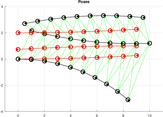
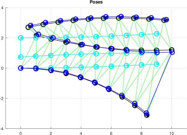
Figure 2: Simulation experiment. Robot poses are shown by circles with a bar indicating the forward direction. Top: Estimated poses (red), true poses (black), and pairs of poses used in homing measurements (dotted green lines). The first lane starts at the origin, subsequent lanes are shifted upwards. Bottom: Result of the Lagrange-Newton descent overlaid on the top figure. Initial state (cyan), final state (blue), pairs of poses used in homing measurements (dotted green lines). (Inter-lane connections in the initial and final states should be ignored.)

8 Conclusions

Our preliminary experiments demonstrate that the suggested method of expressing rotational components through orientation vectors — which are pushed towards unit length by Lagrange constraints — is feasible. It eliminates the need to transform variations between manifolds in each step which is required in the Gauss-Newton approach. An obstacle to an application are the numerical instabilities which occur in a few runs depending on the random errors in the measurements.

We noticed that the initialization of the Lagrange multipliers using (269) seems to be important to achieve fast convergence. Using initialization values far from the solution delays convergence as first the method approaches the constraint before starting to reduce the cost functions. In some runs we observed numerical instabilities if unsuitable initial values were used.

We tested three different types of rotational cost functions with increasing complexity (see section 4.3): the first form (29) with $t_{1}=1$, the first form (29) with $t_{1}=0$, and the second form (28). The simulations show no fundamental differences in performance; we just had the impression that the second form may require Levenberg-Marquardt steps more often, but this needs to be studied in detail. We cautiously conclude that it is (1) not necessary to make the cost function independent of constraint violations and (2) not even necessary to guarantee non-negative costs when the constraints are violated. It would therefore be justified to just use the simplest form of a cost function which has the desired effect when the constraints are fulfilled. Note that the translation error just guarantees non-negativity but not independence of constraint violations; we didn’t explore a version fulfilling the strongest requirement for this cost function.

The methods currently used for line-search and Levenberg-Marquardt regularization are not very sophisticated since they were simplified from the methods suggested in the literature. Also there is no mechanism that modifies the steps far from the solution to accelerate the convergence.

We only tested the method for the setup shown in figure 2; extensive tests with different and larger graphs are required. Moreover, none of the method’s parameters were systematically varied: We didn’t explore the influence of the weight factor for rotational cost functions $\gamma$ (simulations use $\gamma=1$); it is also not clear whether the effect of $\gamma$ is actually removed by the Newton method. We just superficially looked for suitable weight factors for the L1-term in the augmented Lagrangian, for the sets of the two weight factor in the Levenberg-Marquardt regularization, and for the resolution and range of the line-search (see section 6.7).

Finally, we raise the question whether the method can be extended to angles in three dimensions. Presently, our derivation and simulation are restricted to robot movements in the plane. In this case, each angle is expressed by a two-dimensional orientation vector; all rotations are implicitly related to the axis perpendicular to the plane. The lengths of all orientation vectors are pushed towards unity by Lagrange constraints. A two-by-two orientation matrix is formed from an orientation vector to express rotations and projections. In three dimensions, we expect that two vectors are sufficient to express each angle. These would be complemented by a third vector to a Cartesian right-handed coordinate system; the axes of this coordinate system would form the orientation matrix. The Lagrange constraint would enforce that the matrix holding the two orientation vectors in its columns would be semi-orthogonal.

Document Changes

24 Jan 2024: first release

References

• Biegler (2010) L. T. Biegler. Nonlinear Programming. Society for Industrial and Applied Mathematics, 2010.
• Deisenroth et al. (2020) M. P. Deisenroth, A. A. Faisal, and C. S. Ong. Mathematics for Machine Learning. Cambridge University Press, 2020.
• Gerstmayr-Hillen et al. (2013) L. Gerstmayr-Hillen, F. Röben, M. Krzykawski, S. Kreft, D. Venjakob, and R. Möller. Dense topological maps and partial pose estimation for visual control of an autonomous cleaning robot. Robotics and Autonomous Systems, 61(5):497–516, May 2013.
• Grisetti et al. (2010) G. Grisetti, R. Kümmerle, C. Stachniss, and W. Burgard. A tutorial on graph-based SLAM. IEEE Transactions on Intelligent Transportation Systems Magazine, 2(4):31–43, 2010.
• Izmailov and Solodov (2014) A. F. Izmailov and M. V. Solodov. Newton-Type Methods for Optimization and Variational Problems. Springer Series in Operations Research and Financial Engineering. Springer, 2014.
• Laue et al. (2018) S. Laue, M. Mitterreiter, and J. Giesen. Computing higher order derivatives of matrix and tensor expressions. In S. Bengio, H. Wallach, H. Larochelle, K. Grauman, N. Cesa-Bianchi, and R. Garnett, editors, Advances in Neural Information Processing Systems 31 (NeurIPS 2018). 2018.
• Laue et al. (2020) S. Laue, M. Mitterreiter, and J. Giesen. A simple and efficient tensor calculus. Proceedings of the AAAI Conference on Artificial Intelligence, 34(4):4527–4534, 2020.
• Möller et al. (2013) R. Möller, M. Krzykawski, L. Gerstmayr-Hillen, M. Horst, D. Fleer, and J. de Jong. Cleaning robot navigation using panoramic views and particle clouds as landmarks. Robotics and Autonomous Systems, 61(12):1415–1439, 2013.
• Toussaint (2017) M. Toussaint. A tutorial on Newton methods for constrained trajectory optimization and relations to SLAM, Gaussian process smoothing, optimal control, and probabilistic inference. In J.-P. Laumond, N. Mansard, and J.-B. Lasserre, editors, Geometric and Numerical Foundations of Movements, Springer Tracts in Advanced Robotics 117, pages 361–392. Springer International Publishing, Cham, Switzerland, 2017.