Dynamics of non-Hermitian Floquet Wannier-Stark system

Abstract

We study the dynamics of the non-Hermitian Floquet Wannier-Stark system in the framework of the tight-binding approximation, where the hopping strength is a periodic function of time with Floquet frequency $\mathcal{\omega}$. It is shown that the energy level of the instantaneous Hamiltonian is still equally spaced and independent of time $t$ and the Hermiticity of the hopping term. In the case of off resonance, the dynamics are still periodic, while the occupied energy levels spread out at the resonance, exhibiting $t^{z}$ behavior. Analytic analysis and numerical simulation show that the level-spreading dynamics for real and complex hopping strengths exhibit distinct behaviors and are well described by the dynamical exponents $z=1$ and $z=1/2$, respectively.

I Introduction

The Hermitian and static system is the main study object of traditional quantum mechanics, preserving the reality and conservation of energy. When these two constraints are violated, the properties of the material could be drastically modified, leading to new phases and phenomena Moiseyev2011 ; Tannor2007 without analogs in their static or Hermitian counterparts. Floquet engineering has facilitated the exploration of diverse dynamic, topological, and transport phenomena across a wide range of physical contexts. More recently, the Floquet approach has been employed to engineer topological phases in non-Hermitian systems. Importantly, it was discovered that the interplay between time-periodic driving fields and the presence of gain, loss, or nonreciprocal effects can lead to the emergence of topological phases exclusive to non-Hermitian Floquet systems PhysRevB.98.205417 ; PhysRevLett.102.065703 ; LeonMontiel2018 ; Li2019 ; PhysRevA.102.062201 ; Blose2020 ; Zhou2020 ; Zhang2020 ; Xiao2020 ; Ageev2021 .

Motivated by the above investigations, the aim of the present paper is to examine how non-Hermiticity and periodic driving impact a Stark ladder system. Specifically, we study the dynamics of the non-Hermitian Floquet Wannier-Stark system in the framework of the tight-binding approximation. In this work, we introduce non-Hermiticity and periodic driving by focusing on cosinusoidal time-dependent hopping strength with frequency $\mathcal{\ \omega}$ and complex amplitude. The main reason for choosing such systems is that the energy level of the instantaneous Hamiltonian is still equally spaced with $\mathcal{\omega}_{0}$ and independent of time $t$ and the Hermiticity of the hopping strength. It allows us to investigate the dynamics based on analytical solutions. We find that, in the case of off resonance, the dynamics are still periodic, while the occupied energy levels spread out at the resonance, exhibiting $t^{z}$ behavior. Analytic analysis and numerical simulation show that the level-spreading dynamics for real and complex hopping strengths exhibit distinct behaviors and are well described by the dynamical exponents $z=1$ and $z=1/2$, corresponding to superdiffusion and diffusion, respectivelyZhao2006 ; metzler1999anomalous ; Bouchaud1990 . These findings may help us deepen our understanding of the interplay between non-Hermiticity and periodic driving impacts on the dynamics of the system. In addition, we propose a scheme to demonstrate the results by wavepacket dynamics in a $2$D square lattice.

This paper is organized as follows. In Sec. II, we introduce a non-Hermitian time-dependent tight-binding model supporting a Wannier-Stark ladder and present the analytical eigenstates of the instantaneous Hamiltonian. In Sec. III, we focus on the dynamics of the static system, while the Floquet system at resonance in Sec. IV. Sec. V describes the application of the solutions to a specific initial state. In Sec. VI, a scheme for the simulator of our results is proposed in the framework of wavepacket dynamics in a $2$D square lattice. Finally, we summarize our results in Sec. VII.

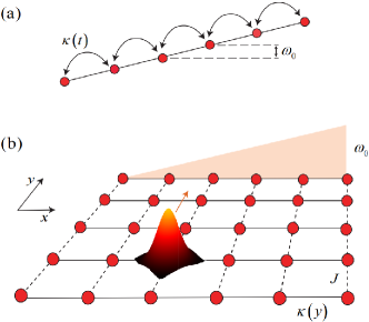
Figure 1: (a) Schematic illustrations of the Hamiltonian in Eq. (1), which represents a tight-binding chain with a time dependence on the hopping strength between two adjacent sites. The on-site potential is tilted with slope $\omega_{0}$. It is shown that such a system supports a Stark-ladder with time-independent energy-level spacing. (b) Schematic illustrations for the Hamiltonian in Eq. (43), which is a tight-binding model of a square lattice with time-independent system parameters. The contributions of hopping strength and on-site potential can be used to simulate the dynamics of system (a).

II Model and generalized Wannier-Stark ladder

We start with the tight-binding model with the Hamiltonian

$$H=\kappa(t)\sum\limits_{n=-\infty}^{+\infty}(|n\rangle\langle n+1|+\text{ {H.c}})+\mathcal{\omega}_{0}\sum\limits_{n=-\infty}^{+\infty}n|n\rangle\langle n|,$$ (1)

where $|n\rangle$ denotes a site state describing the Wannier state localized on the $n$th period of the potential. Here, $\kappa(t)$ is the time-dependent tunneling strength, while $\mathcal{\omega}_{0}$ is the slope of the linear potential from a static force. Fig. 1(a) shows a schematic of the system. In our study, $\kappa$ can be real and complex. It is well known that the spectrum of $H$ is equally spaced when $\kappa$ is a real constant, supporting periodic dynamics Hartmann2004 ; bloch1928elektron ; 1934 . This has been observed in systems of semiconductor superlattices and ultracold atoms Waschke1993 ; BenDahan1996 ; Wilkinson1996 ; Anderson1998 .

Now, we extend the conclusion to the case with arbitrary $\kappa$. The eigenstate of $\left|\psi_{n}\right\rangle$ can always be written in the form

$$\left|\psi_{n}\right\rangle=\sum_{m}c_{mn}|m\rangle,$$ (2)

satisfying the Schrodinger equation

$$H\left|\psi_{n}\right\rangle=E_{n}\left|\psi_{n}\right\rangle.$$ (3)

The coefficient $c_{mn}$ is determined by the equation

$$c_{m+1,n}+c_{m-1,n}=\frac{E_{n}-m\mathcal{\omega}_{0}}{\kappa}c_{mn},$$ (4)

which accords with the recurrence relation of the Bessel function $J_{m}$ of argument $x$, i.e.,

$$J_{m+1}(x)+J_{m-1}(x)=2\frac{m}{x}J_{m}(x).$$ (5)

Then, we have

$$c_{mn}=J_{m-n}(-\frac{2\kappa}{\omega_{0}}),E_{n}=n\omega_{0}.$$ (6)

We can see that the eigenenergy $n\mathcal{\omega}_{0}$ is independent of $\kappa$, regardless of whether it is real or complex. This is crucial for the main conclusion of this work. Although the profile of the eigenstate

$$\psi_{m}\left(n\right)=\langle n|\psi_{m}\rangle=J_{n-m}(-\frac{2\kappa}{\omega_{0}}),$$ (7)

in real space is $\kappa$ dependent, and it is always localized. The inverse participation ratio (IPR) is a simple way to quantify the localization of a given state. For spatially extended states, the value of the IPR approaches zero when the system is sufficiently large, whereas it is finite for localized states regardless of the system size. The IPR of the eigenstate $\left|\psi_{m}\right\rangle$ is

$$\text{IPR}_{m}=\frac{\sum\limits_{n}\left|\langle n|\psi_{m}\rangle\right|^{4}}{\sum\limits_{n}\left|\langle n|\psi_{m}\rangle\right|^{2}}=\sum_{n}|J_{n-m}(-\frac{2\kappa}{\omega_{0}})|^{4}.$$ (8)

Numerical simulations show that IPR_m is independent of $m$ and $N$ for a sufficiently large $N$. We have IPR${}_{m}=0.418$ and $1.217$ for $-2\kappa/\omega_{0}=1.0$ and $1.0i$, respectively, which indicates that $\left|\psi_{m}\right\rangle$ is in a localized state. In parallel, without loss of generality, we have

$$\left|\varphi_{m}\right\rangle=\sum_{n}J_{n-m}(-\frac{2\kappa^{\ast}}{\omega_{0}})|n\rangle,$$ (9)

for the equation

$$H^{{\dagger}}\left|\varphi_{m}\right\rangle=m\omega_{0}\left|\varphi_{m}\right\rangle,$$ (10)

which establishes the biorthonormal set $\left\{|\varphi_{m}\rangle,|\psi_{n}\rangle\right\}$, satisfying

$$\langle\varphi_{m}\left|\psi_{n}\right\rangle=\sum_{n^{\prime}}J_{n^{\prime}-m}^{\ast}(-\frac{2\kappa^{\ast}}{\omega_{0}})J_{n^{\prime}-n}(-\frac{2\kappa}{\omega_{0}})=\delta_{mn},$$ (11)

since the eigenlevels are independent of $\kappa$, without coalescence of eigenvectors. This is an important basis for the following investigations.

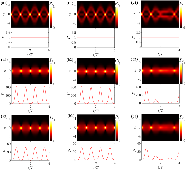
Figure 2: Plots of $P_{n}(t)$ and $P(t)$ defined in Eqs. (15 ) and (16), obtained by numerical diagonalization for several typical values of system parameters with $\mathcal{\omega}_{0}=1$. Here, (a1), (b1), and (c1) correspond to the cases with $\omega=0$, $0.01$, and $0.1$, respectively, and $\kappa_{0}=1$. (a2), (b2), and (c2) correspond to the cases with $\omega=0$, $0.01$, and $0.1$, respectively, and $\kappa_{0}=i$. (a3), (b3),and (c3) correspond to the cases with $\omega=0$, $0.01$, and $0.1$, respectively, and $\kappa_{0}=e^{i\pi/4}$.

III Bloch oscillation in non-Hermitian system

Now, we consider the dynamics of the system with slowly varying $\kappa(t)$. When $\kappa$ is time independent, the dynamics of the system are governed by the propagator

$$U_{mn}\left(t\right)=\langle m|e^{-iHt}|n\rangle.$$ (12)

Employing the biorthonormal set $\left\{|\varphi_{m}\rangle,|\psi_{n}\rangle\right\}$, we have

$$U_{mn}\left(t\right)=\sum_{l}\langle m|\psi_{l}\rangle e^{-iE_{l}t}\langle\varphi_{l}|n\rangle$$ (13)

$$= J_{m-n}(-\frac{4\kappa}{\omega_{0}}\sin\frac{\omega_{0}t}{2})e^{-i(m-n)\frac{\omega_{0}t}{2}}i^{m-n}e^{-in\omega_{0}t},$$

$$= i^{m-n}e^{-i(m+n)\frac{\omega_{0}t}{2}}J_{m-n}(-\frac{4\kappa}{\omega_{0}}\sin\frac{\omega_{0}t}{2}),$$

which is a periodic function with period $2\pi/\omega_{0}$. For a given initial state

$$\left|\Phi(0)\right\rangle=\sum_{l}c_{l}|l\rangle$$ (14)

the Dirac probability distribution in real space for the evolved state $\left|\Phi(t)\right\rangle$ is

$$P_{m}(t)=\left|\langle m\left|\Phi(t)\right\rangle\right|^{2}=\left|\sum_{l}c_{l}U_{ml}\left(t\right)\right|^{2},$$ (15)

which is still periodic. We obtain the conclusion that the total Dirac probability

$$P(t)=\sum_{n}P_{n}(t),$$ (16)

is still periodic, regardless of whether $\kappa$ is real or complex.

In this work, we explore what happens when $\kappa$ is time dependent. According to the adiabatic theorem, the expression of $U_{mn}\left(t\right)$ still holds true for slowly varying $\kappa(t)$ during a short period of time. Considering the case with $\kappa(t)=\kappa_{0}\cos(\omega t)$, where $\kappa_{0}$ can be a complex number and the frequency of $\kappa$ is small, $\mathcal{\omega}\ll\mathcal{\omega}_{0}$. It can be predicted that $\left|\Phi(t)\right\rangle$ and $P(t)$ are still approximately periodic even for the quasiadiabatic process. However, this approach could be invalid for the diabatic process.

To verify and demonstrate the above analysis, numerical simulations are performed to investigate the dynamic behavior of dynamic processes with different values of $\mathcal{\omega}/\mathcal{\omega}_{0}$. We compute the temporal evolution of a site state, $\left|\Phi(0)\right\rangle=|0\rangle$ by using a uniform mesh in the time discretization for the time-dependent Hamiltonian $H(t)$. The evolved state is

$$\left|\Phi(t)\right\rangle=\mathcal{T}\exp\left[-i\int_{0}^{t}H\left(t\right)\mathrm{d}t\right]\left|\Phi(0)\right\rangle,$$ (17)

where $\mathcal{T}$ is the time-order operator. Fig. 2 shows the plots of $P_{n}(t)$ and $P(t)$ for several typical values of $\mathcal{\omega}/\mathcal{\omega}_{0}$.

The numerical results indicate that the Bloch oscillation exists for small $\mathcal{\omega}/\mathcal{\omega}_{0}$. For non-Hermitian cases, the profile of the evolved state does not change substantially, but the probability is periodic or quasiperiodic.

IV Floquet-resonance dynamics

Now, we investigate the dynamics of the system with time-dependent $\kappa(t)$. When $\kappa(t)$ is periodic, the system becomes a Floquet system. The solution of the Schrödinger equation

$$i\frac{\partial}{\partial t}|\Psi\left(t\right)\rangle=H(t)|\Psi(t)\rangle$$ (18)

can be written in the form

$$|\Psi(t)\rangle=\sum_{m}a_{m}(t)e^{-im\mathcal{\omega}_{0}t}|\psi_{m}\rangle,$$ (19)

where the coefficient $a_{n}$ obeys the following equation:

$$\frac{\partial a_{m}}{\partial t}=-\sum_{n}a_{n}e^{i\left(m-n\right)\omega_{0}t}\left\langle\varphi_{m}\right|\frac{\partial}{\partial t}|\psi_{n}\rangle.$$ (20)

Submitting the expression of $|\varphi_{m}(t)\rangle$ and $|\psi_{n}(t)\rangle$, we have

$$\frac{\partial a_{n}}{\partial t}=\frac{1}{\omega_{0}}\frac{\partial\kappa}{\partial t}(a_{n-1}e^{i\mathcal{\omega}_{0}t}-a_{n+1}e^{-i\mathcal{\omega}_{0}t}),$$ (21)

which is the starting point for the following discussions.

In this work, we consider the case with $\kappa(t)=\kappa_{0}\cos(\omega t)$, where $\kappa_{0}$ can be a complex number. Taking the rotating-wave approximation (RWA) under the condition $\left|\mathcal{\omega}-\mathcal{\omega}_{0}\right|\ll\mathcal{\omega}_{0}$, we have

$$i\frac{\partial a_{n}}{\partial t}=\frac{\kappa_{0}\omega}{2\omega_{0}}[a_{n-1}e^{i(\mathcal{\omega}_{0}-\omega)t}+a_{n+1}e^{i(\omega-\mathcal{\ \omega}_{0})t}].$$ (22)

We focus on the dynamics of the system at resonance $\mathcal{\omega}=\mathcal{\omega}_{0}$, in which the equation becomes

$$i\frac{\partial a_{n}}{\partial t}=\frac{\kappa_{0}}{2}(a_{n-1}+a_{n+1}).$$ (23)

The Schrödinger equation is used for a uniform tight-binding chain.

V Dynamical exponents

As shown above, the resonant dynamics are essentially governed by the simple equivalent Hamiltonian

$$H_{\mathrm{eq}}=\frac{\kappa_{0}}{2}\sum\limits_{n=-\infty}^{+\infty}(|n\rangle\langle n+1|+\text{{H.c}}),$$ (24)

where $|n\rangle$ denotes the eigenstates of the instantaneous Hamiltonian. The Hamiltonian $H_{\mathrm{eq}}$ can be diagonalized in the form

$$H_{\mathrm{eq}}=\sum\limits_{k\in(-\pi,\pi)}\varepsilon_{k}|k\rangle\langle k|,$$ (25)

with

$$|k\rangle=\frac{1}{\sqrt{2\pi}}\sum\limits_{l}e^{ikl}|l\rangle,$$ (26)

and the spectrum

$$\varepsilon_{k}=\kappa_{0}\cos k.$$ (27)

The time evolution of state

$$\left|\Psi(t)\right\rangle = \sum\limits_{l}a_{l}(t)|l\rangle$$ (28)

$$= \sum\limits_{l}a_{l}(0)\sum_{n}i^{n-l}J_{n-l}(-\kappa_{0}t)|n\rangle,$$

can be obtained for any given $\left\{a_{l}(0)\right\}$. Intuitively, an initial state $|0\rangle$ (or $a_{l}(0)=\delta_{0l}$) could spread out and never return whether $\kappa_{0}$ is real or complex. In the following, we focus on two cases with $\kappa_{0}=1$ and $\kappa_{0}=i$.

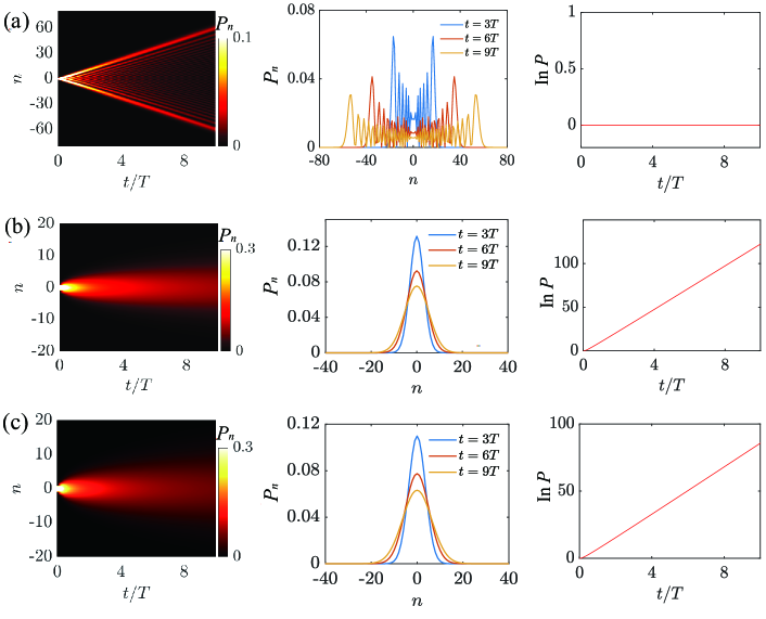
Figure 3: The same plots of $P_{n}(t)$ and $P(t)$ as those in Fig. 2 are shown for several typical values of system parameters but at a resonance $\mathcal{\omega}_{0}=\omega=1$. Here, (a), (b), and (c) correspond to the cases with $\kappa_{0}=1$, $i$, and $e^{i\pi/4}$, respectively. The middle panels correspond to the probability distributions at moments $t=3T$, $6T$, and $9T$, respectively. The right panels are the logarithmic plots of total probabilities as functions of time. These results accord with our analytical analysis in the main text.

(i) $\kappa_{0}=1$; in this case, the straightforward derivation yields

$$a_{n}(t)=i^{n}J_{n}(-t),$$ (29)

which ensures the probability distribution of the energy levels

$$\mathcal{P}_{n}(t)=\left|a_{n}(t)\right|^{2}=\left|J_{n}(-t)\right|^{2},$$ (30)

and

$$\mathcal{P}=\sum\limits_{n}\mathcal{P}_{n}(t)=1.$$ (31)

The feature of the Bessel function tells us that there exists a maximum at the edge of $\mathcal{P}_{n}(t)$, which can be regarded as the wave front of the occupied-energy-level spreading. The location of such a wave front can then be determined by the equation

$$\frac{\partial\mathcal{P}_{m_{c}}(t)}{\partial t}=0.$$ (32)

Based on the relations $J_{n-1}(x)-J_{n+1}(x)=2J_{n}^{\prime}(x)$ and $J_{m_{c}+1}\left(-t\right)+J_{m_{c}-1}\left(-t\right)=2\left|m_{c}/t\right|J_{m_{c}}\left(-t\right),$ we have

$$2J_{m_{c}+1}(-t)=2|m_{c}/t|J_{m_{c}}(-t).$$ (33)

For large $n$ and $t$, we have $J_{m_{c}+1}(-t)\approx J_{m_{c}}(-t)$, which results in

$$|m_{c}|\approx t.$$ (34)

Then, we conclude that the dynamical exponent of occupied-energy-level spreading is $z=1$.

(ii) $\kappa_{0}=i$; in parallel, the corresponding amplitude is the Bessel function with imaginary argument

$$a_{2n}(t) = (-1)^{n}J_{2n}(-it)$$ (35)

$$= \frac{(-1)^{n}}{2\pi}\int_{-\pi}^{\pi}\cos(2nk)e^{-t\sin k}\mathrm{d}k,$$

and

$$a_{2n+1}(t) = i(-1)^{n}J_{2n+1}(-it)$$ (36)

$$= \frac{(-1)^{n+1}}{2\pi i}\int_{-\pi}^{\pi}\sin[(2n+1)k]e^{-t\sin k}\mathrm{d}k.$$

On a long time scale, the main contribution to the integral comes from the integrand around $k=-\pi/2$. Then, we have

$$a_{2n}(t)\approx e^{-\frac{(2n)^{2}}{t}}\frac{1}{2\pi}\int_{-\pi}^{\pi}e^{-t\sin k}\mathrm{d}k,$$ (37)

and

$$a_{2n+1}(t)\approx e^{-\frac{(2n+1)^{2}}{t}}\frac{1}{2\pi i}\int_{-\pi}^{\pi}e^{-t\sin k}\mathrm{d}k,$$ (38)

with small $\varepsilon_{k}$, which results in the probability distribution of the energy levels

$$\mathcal{P}_{n}(t)=|a_{n}(t)|^{2}\approx\sqrt{\frac{2}{\pi t}}\mathcal{P}e^{-\frac{2n^{2}}{t}},$$ (39)

with the total probability

$$\mathcal{P}=\sum_{n}\mathcal{P}_{n}=\frac{1}{2\pi}\int_{-\pi}^{\pi}e^{-2t\sin k}\mathrm{d}k.$$ (40)

Obviously, the profile of $\mathcal{P}_{n}$ is a Gaussian type, and the total probability grows exponentially as $e^{2t}$ approaches the large $t$ limit. In this situation, the dynamics of occupied-energy-level spreading can be characterized by the full width at half maximum (FWHM),

$$\mathcal{P}_{n_{c}}(t)=\frac{1}{2}\mathcal{P}_{0}(t),$$ (41)

which results in

$$|n_{c}|\approx\sqrt{t}.$$ (42)

Then, we conclude that the dynamical exponent of occupied-energy-level spreading is $z=1/2$.

To verify and demonstrate the above analysis, numerical simulations are performed to investigate the dynamic behavior of dynamic processes at resonance with $\mathcal{\omega}=\mathcal{\omega}_{0}$. For the same initial state as shown in Fig. 2, the plots of $P_{n}(t)$ and $P(t)$ for several typical values of $\kappa_{0}$  are presented in Fig. 3. These numerical results accord with our above analysis in two aspects: (i) At resonance, the dynamics are no longer periodic; (ii) The level spreading exhibits distinct behaviors for Hermitian and non-Hermitian systems.

VI 2D simulator via wavepacket dynamics

In this section, we will show how the time evolution of a wavepacket in an engineered time-independent 2D square lattice can simulate our results for Floquet dynamics in a 1D time-dependent lattice. In experiments, single-particle hopping dynamics can be simulated by discretized spatial light transport in an engineered 2D square lattice of evanescently coupled optical waveguides Christodoulides2003 . A 2D lattice can be fabricated by coupled waveguides, by which the temporal evolution of the single-particle probability distribution in the 2D lattice can be visualized by the spatial propagation of the light intensity.

We consider a single-particle Hamiltonian on a square lattice

$$H_{\mathrm{2D}} = \kappa_{0}\sum_{n,m=-\infty}^{\infty}\cos\left(qm\right)|n,m\rangle\langle n+1,m|$$ (43)

$$-J\sum_{n,m=-\infty}^{\infty}|n,m\rangle\langle n,m+1|+\mathrm{h.c.}$$

$$+\omega_{0}\sum_{n,m=-\infty}^{\infty}n|n,m\rangle\langle n,m|,$$

which is an array of coupled 1D Bloch systems with $q$-dependent hopping strength $\kappa_{0}\cos\left(qm\right)$. Fig. 1(b) shows a schematic of the system. According to the above analysis, the system is governed by Bloch dynamics with frequency $\omega_{0}$ for vanishing $J$, regardless of whether $\kappa_{0}$ is real or complex.

Figure 4: For numerical simulations of the dynamics, the trajectories of wavepackets evolving in the in a 2D lattice with four typical configurations were obtained. The traces of the wavepacket $P(n,m)$ for the time evolutions of the four cases are shown in (a1), (b1), (c1), and (d1). Probability distributions $p(n,m,t)$ for the time evolutions of four representative cases at $t=0$, $t=2\pi/J$, $t=4\pi/J$, $t=6\pi/J$ and $t=8\pi/J\,$are shown in (a2), (b2), (c2), and (d2), respectively. The initial states and system parameters are given in the main text. The size of the system is $60\times 30$. The energy scale of the Hamiltonian is taken as $J=1$. The probability distributions on the square lattice exhibit distinct patterns corresponding to the dynamic behaviors of Bloch breathing, oscillation, diffusion and superdiffusion.

Now, we start to investigate the dynamics in the presence of nonzero $J$. The $k$-space representation of the Schrödinger equation

$$i\frac{\partial}{\partial t}|\psi\rangle=H|\psi\rangle,$$ (44)

can be written as

$$i\frac{\partial\psi}{\partial t} = \kappa_{0}\cos k_{x}[\psi\left(k_{x},k_{y}+q,t\right)+\psi\left(k_{x},k_{y}-q,t\right)]$$ (45)

$$+i\omega_{0}\frac{\partial\psi}{\partial k_{x}}-2J\cos k_{y}\psi\left(k_{x},k_{y},t\right),$$

by taking the Fourier transformation

$$|k_{x},k_{y}\rangle=\frac{1}{2\pi}\sum_{n,m=-\infty}^{\infty}e^{i\left(k_{x}n+k_{y}m\right)}|n,m\rangle.$$ (46)

For the case with $q=0$, the solution $\psi\left(k_{x},k_{y},t\right)$ reduces to

$$\psi\left(k_{x},k_{y},t\right)=f\left(k_{x},t\right)e^{it2J\cos k_{y}},$$ (47)

where $f\left(k_{x},t\right)$ obeys the following equation:

$$i\frac{\partial f}{\partial t}=(2\kappa_{0}\cos k_{x}+i\omega_{0}\frac{\partial}{\partial k_{x}})f\left(k_{x},t\right).$$ (48)

In the case with $k_{y}\approx\pi/2$, we have $\cos k_{y}\approx k_{y}-\pi/2$. One can construct a solution by the superposition of states $|k_{x},k_{y}\rangle$ with $k_{y}\approx\pi/2$ in the form Kim2006

$$\left|g\left(k_{x},t\right)\right\rangle = (\frac{2\alpha^{2}}{\pi})^{1/4}\int_{-\pi}^{\pi}e^{-\alpha^{2}\left(k_{y}-\pi/2\right)^{2}}e^{it2J\cos k_{y}}$$ (49)

$$\times f\left(k_{x},t\right)\mathrm{d}k_{y}|k_{x},k_{y}\rangle$$

$$\approx (\frac{1}{2\pi\alpha^{2}})^{1/4}\sum_{m}e^{im\pi/2}e^{-(1/4)(m-2Jt)^{2}/\alpha^{2}}$$

$$\times f\left(k_{x},t\right)|k_{x},m\rangle,$$

which is a traveling Gaussian wavepacket in the $y$ direction. It is presumed that such a solution still holds true by taking $\kappa_{0}\rightarrow\kappa_{0}\cos\left(qm\right)$ when $\kappa_{0}\cos\left(qm\right)$ varies slowly during the extension of the wavepacket in the y direction due to the locality of the solution. In this sense, the traveling wavepacket experiences an adiabatic process, after which the independence of the dynamics in both directions is maintained. Obviously, a small value of q should be needed. On the other hand, the value of $\omega_{0}$ must match $q$ when the system is employed to simulate the dynamics at the resonance. To this end, a small value of $\kappa_{0}$ should be taken to maintain the Stark ladder.

Actually, under the conditions $\kappa_{0}\ll J$ and $k_{y}\approx\pi/2$, such a 2D system is equivalent to a coupled waveguide array due to the linear dispersion in the $y$ direction, in which the tunneling rate between neighboring waveguides is $m$ dependent. The speed of the propagating wavepacket along $m$ is $2J$. To simulate the dynamics along $x$, one can simply take $q=\omega/\left(2J\right)$, regarding $m$ as the temporal coordinate.

To determine the dynamics of the square lattice system, we perform numerical simulations. We compute the time evolutions for the initial state in the form

$$\psi(n,m,0)=(\frac{1}{4\pi^{2}\alpha^{4}})^{1/4}e^{im\pi/2}e^{-(1/4)(m^{2}+n^{2})/\alpha^{2}},$$ (50)

in the following four representative cases. (i) To simulate Bloch breathing, the initial state is taken as $\psi(0,m,0)\delta_{n,n_{0}}$ with $\alpha=1$. The system parameters are $\kappa_{0}=J$, $\omega=0$ and $\omega_{0}=0.5J$. (ii) To simulate Bloch oscillation, the initial state is taken as $\psi(n,m,0)$ with $\alpha=1$. The system parameters are $\kappa_{0}=J$, $\omega=0$ and $\omega_{0}=0.5J$. (iii) To simulate superdiffusion, the initial state is taken as $\psi(0,m,0)\delta_{n,n_{0}}$ with $\alpha=1$. The system parameters are $\kappa_{0}=0.25J$ and $\omega=\omega_{0}=0.5J$. (iv) To simulate diffusion, the initial state is taken as $\psi(0,m,0)\delta_{n,n_{0}}$ with $\alpha=1$. The system parameters are $\kappa_{0}=0.25Ji$ and $\omega=\omega_{0}=0.5J$. The evolved state has the form

$$\left|\psi\left(n,m,t\right)\right\rangle=e^{-iH_{\mathrm{2D}}t}\left|\psi\left(n,m,0\right)\right\rangle,$$ (51)

which can be computed by exact diagonalization.

The probability distribution at position $(n,m)$ at time $t$ is defined by the Dirac probabilities

$$p(n,m,t)=\left|\langle n,m,\left|\psi\left(n,m,t\right)\right\rangle\right|^{2}.$$ (52)

To visualize the profile of the dynamics, we define the function

$$P(n,m)=\sum_{j=1}p(n,m,j\tau),$$ (53)

to record the trace of the wavepacket. Here, we use $j\tau$ to denote the discretized time coordinate. It is expected that the distribution of $P(n,m)$  exhibits patterns similar to those in Fig. 3. The numerical results presented in Fig. 4 show that the probability distributions on the square lattice exhibit distinct patterns corresponding to the dynamic behaviors of Bloch breathing, oscillation, diffusion and superdiffusion.

VII Summary

In summary, we simultaneously examine the effects of non-Hermiticity and periodic driving on a Stark ladder system. The most fascinating and important feature of such systems is that the Stark ladder can be maintained regardless of the non-Hermiticity of the hopping strength, and the energy level spacing depends only on its norm. This allows us to solve the problem in an analytical manner. The Bloch oscillation is broken when the Floquet frequency is resonant with the energy level spacing, and the occupied energy levels spread out. Furthermore, analytic analysis and numerical simulation show that the level-spreading dynamics for real and complex hopping strengths exhibit distinct behaviors of superdiffusion and diffusion, respectively. In addition, we propose a scheme to simulate the results by wavepacket dynamics in a 2D square lattice. This can be experimentally realized in the coupled array of waveguides. These findings may help us deepen our understanding of the interplay between non-Hermiticity and periodic driving impacts on the dynamics of the system.

- (1) Moiseyev N. Non-Hermitian Quantum Mechanics. Cambridge University Press, 2011.
- (2) D. J. Tannor. Introduction to Quantum Mechanics: A time-dependent perspective. University Science Books, USA, 2007.
- (3) Longwen Zhou and Jiangbin Gong. Non-hermitian floquet topological phases with arbitrarily many real-quasienergy edge states. Phys. Rev. B, 98:205417, Nov 2018.
- (4) M. S. Rudner and L. S. Levitov. Topological transition in a non-hermitian quantum walk. Phys. Rev. Lett., 102:065703, Feb 2009.
- (5) Roberto de J. León-Montiel, Mario A. Quiroz-Juárez, Jorge L. Domínguez-Juárez, Rafael Quintero-Torres, José L. Aragón, Andrew K. Harter, and Yogesh N. Joglekar. Observation of slowly decaying eigenmodes without exceptional points in floquet dissipative synthetic circuits. Commun. Phys., 1(1), December 2018.
- (6) Jiaming Li, Andrew K. Harter, Ji Liu, Leonardo de Melo, Yogesh N. Joglekar, and Le Luo. Observation of parity-time symmetry breaking transitions in a dissipative floquet system of ultracold atoms. Nat. Commun., 10(1), February 2019.
- (7) Peng He and Ze-Hao Huang. Floquet engineering and simulating exceptional rings with a quantum spin system. Phys. Rev. A, 102:062201, Dec 2020.
- (8) Elizabeth Noelle Blose. Floquet topological phase in a generalized -symmetric lattice. Phys. Rev. B, 102(10):104303, September 2020.
- (9) Longwen Zhou. Non-hermitian floquet topological superconductors with multiple majorana edge modes. Phys. Rev. B, 101(1):014306, January 2020.
- (10) Xizheng Zhang and Jiangbin Gong. Non-hermitian floquet topological phases: Exceptional points, coalescent edge modes, and the skin effect. Phys. Rev. B, 101(4):045415, January 2020.
- (11) Lei Xiao, Tianshu Deng, Kunkun Wang, Gaoyan Zhu, Zhong Wang, Wei Yi, and Peng Xue. Non-hermitian bulk–boundary correspondence in quantum dynamics. Nat. Phys., 16(7):761–766, March 2020.
- (12) Dmitry S. Ageev, Andrey A. Bagrov, and Askar A. Iliasov. Deterministic chaos and fractal entropy scaling in floquet conformal field theories. Phys. Rev. B, 103(10):l100302, March 2021.
- (13) Hong Zhao. Identifying diffusion processes in one-dimensional lattices in thermal equilibrium. Phys. Rev. Lett., 96(14):140602, April 2006.
- (14) Ralf Metzler, Eli Barkai, and Joseph Klafter. Anomalous diffusion and relaxation close to thermal equilibrium: A fractional fokker-planck equation approach. Phys. Rev. Lett., 82(18):3563, 1999.
- (15) Jean-Philippe Bouchaud and Antoine Georges. Anomalous diffusion in disordered media: Statistical mechanisms, models and physical applications. Phys. Rep., 195(4–5):127–293, November 1990.
- (16) T Hartmann, F Keck, H J Korsch, and S Mossmann. Dynamics of bloch oscillations. New J. Phys., 6:2–2, January 2004.
- (17) F Bloch. Elektron im periodischen potential, bändermodell des festkörpers, z. Phys, 52:555, 1928.
- (18) Proc. R. soc. Lond. Ser. A-Contain. Pap. Math. Phys. Character., 145(855):523–529, July 1934.
- (19) Christian Waschke, Hartmut G. Roskos, Ralf Schwedler, Karl Leo, Heinrich Kurz, and Klaus Köhler. Coherent submillimeter-wave emission from bloch oscillations in a semiconductor superlattice. Phys. Rev. Lett., 70(21):3319–3322, May 1993.
- (20) Maxime Ben Dahan, Ekkehard Peik, Jakob Reichel, Yvan Castin, and Christophe Salomon. Bloch oscillations of atoms in an optical potential. Phys. Rev. Lett., 76(24):4508–4511, June 1996.
- (21) S. R. Wilkinson, C. F. Bharucha, K. W. Madison, Qian Niu, and M. G. Raizen. Observation of atomic wannier-stark ladders in an accelerating optical potential. Phys. Rev. Lett., 76(24):4512–4515, June 1996.
- (22) B. P. Anderson and M. A. Kasevich. Macroscopic quantum interference from atomic tunnel arrays. Science, 282(5394):1686–1689, November 1998.
- (23) Demetrios N. Christodoulides, Falk Lederer, and Yaron Silberberg. Discretizing light behaviour in linear and nonlinear waveguide lattices. Nature, 424(6950):817–823, August 2003.
- (24) Wonkee Kim, L. Covaci, and F. Marsiglio. Impurity scattering of wave packets on a lattice. Phys. Rev. B, 74(20):205120, November 2006.