$\nu$Oscillation: a software package for computation and simulation of neutrino propagation and interaction

Abstract

The behavior of neutrinos is the only phenomenon that cannot be explained by the standard model of particle physics. Because of these mysterious neutrino interactions observed in nature, at present, there is growing interest in this field and ongoing or planned neutrino experiments are seeking solutions to this mystery very actively. The design of neutrino experiments and the analysis of neutrino data rely on precise computations of neutrino oscillations and scattering processes in general. Motivated by this, we developed a software package that calculates neutrino production and oscillation in nuclear reactors, neutrino-electron scattering of solar neutrinos, and the oscillation of neutrinos from radioactive isotopes for the search of sterile neutrinos. This software package is validated by reproducing the result of calculations and observations in other publications. We also demonstrate the feasibility of this package by calculating the sensitivity of a liquid scintillator detector, currently in planning, to the sterile neutrinos. This work is expected to be used in designs of future neutrino experiments.

I Introduction

The standard model (SM) of particle physics ref:SM ; ref:SM2 ; ref:SM3 ; ref:SM4 ; ref:QCD ; ref:qcd2 describing the electroweak and strong nuclear interactions of subatomic particles in microscopic scales has been validated almost over a half-century extremely successfully, consistent with its prediction, except for one notable exceptional deviation in the neutrino sector. The SM predicts that neutrinos are precisely massless, yet experiments  ref:superK_atmos ; ref:sno2001 ; ref:kamland ; ref:SNO2 indicate that neutrinos have small but finite mass values, allowing quantum oscillations among eigenstates of the weak force in subatomic particle interaction. In order to search for solutions to this one of profound fundamental problems in modern particle physics, tremendous efforts are focused, on ongoing and future neutrino experiments ref:hyperkamiokande ; ref:dune , not to mention previous precious experiments. These experimental efforts often require computation of neutrino production, propagation, and interaction with matter at different experimental conditions such as nuclear reactors, solar, accelerator, or radioactive source-based environments.

For the detailed study of the phenomena with neutrinos, there have been number of software packages developed to calculate the interaction and propagation of neutrinos ref:n_packages ; ref:n_packages2 and references therein. A large number of existing packages are theoretically oriented, mathematically very rigorous, and focused on the calculation of given Hamiltonian, including non-standard interactions. For feasibility study and design optimization of future experiments, a software tool that also offers enough precision and flexibility is desired to carry out detailed studies on future neutrino experiments.

Motivated by these, we developed a unified software package, the $\nu$Oscillation, which calculates neutrino production and oscillation in nuclear reactors, neutrino-electron scattering of the neutrinos originating from the Sun, and the oscillation of SM neutrinos from radioactive isotopes to hypothetical non-SM sterile neutrinos. This work is expected to be utilized to identify the physics potential and in the design optimization of future neutrino experiments.

II Implementation of the Software

At present, observed neutrinos appear to be point-like, spin $1/2$ elementary particles and to have three different kinds, commonly called flavours, in their weak interactions with matter. Because of aforementioned their non-zero values of mass, the relation between flavour and mass eigenstates of neutrinos are different and their relations are commonly described by the lepton mixing matrix, known as the Pontecorvo–Maki–Nakagawa– Sakata (PMNS) matrix ref:pmns

$$|\nu_{\alpha}\rangle=\sum_{i}U^{*}_{\alpha i}|\nu_{i}\rangle,$$ (1)

where the flavour index $\alpha$ is $e,\mu$ or $\tau$, the mass index $i$ runs over $1,2,3$, and $U_{\alpha i}$ are elements of the PMNS matrix. The time-evolution of Eq. (1), can be described by time-dependent Schrödinger equation, naturally involve mixing of flavour eigenstates as the given system evolves, and is referred to as the neutrino oscillation. The probability amplitude for the neutrino of flavour $\alpha$ to oscillate into a different flavour $\beta$ at the time $t$ is given by $\langle\nu_{\beta}|\nu(t)\rangle$, providing an oscillation probability

$$P(\nu_{\alpha}\rightarrow\nu_{\beta})=|\langle\nu_{\beta}|\nu_{\alpha}(t)\rangle|^{2}=\Bigg{|}\sum_{i}U_{\beta i}U^{*}_{\alpha i}e^{-iE_{i}t}\Bigg{|}^{2}$$ (2)

where $E_{i}$ is the energy of the $i$-th mass eigenstate. Our package, $\nu$Oscillation computes Eq. (2) at the ultra-relativistic limit of neutrinos, and for our computation, we use analytic expressions in Ref. ref:Zito .

Our implementation of the software, $\nu$Oscillation mainly computes the time evolution of Eq. (1) in given initial conditions set by users. The $\nu$Oscillation also contains computation of inverse beta decay (IBD) cross section, neutrino-electron scattering cross section, and the flux of anti-neutrinos from nuclear reactors, and neutrinos from the Sun, in order to be flexible to different experimental scenarios. We also include one type of fictitious sterile neutrino in the computation of time-evolution of neutrinos as an option to study the sensitivity of the sterile neutrino search on proposed experiments.

Our code is written in C++ implemented as C++ header and source codes utilizing libraries in ROOT ref:root , one of the open-source data analysis frameworks actively used in the field of particle physics. Note also that the ROOT is the de facto standard analysis framework for the experimental high energy physics community. Intended users of $\nu$Oscillation are required to install ROOT along with $\nu$Oscillation, but nothing more. This allows users to utilize $\nu$Oscillation on any operating system that supports ROOT. The source code can be provided upon request.

The $\nu$Oscillation package has the following structure as shown in Fig. 1. The vOscillation class has functions and variables to compute neutrino oscillations based on the PMNS matrix, and its subclass, vSterile introduces sterile neutrinos in the oscillation based on so-called (3+1) model. Note that the vSterileEE class is a simplified implementation of the (3+1) model accounting only the electron flavour initial state. Users can freely set the neutrino oscillation parameters such as $\Delta m^{2}_{ji}$ and $\theta_{ij}$ where $(i,j)$ can be $(1,2),(1,3)$ or $(2,3)$. Here, $\Delta m^{2}_{ji}$ and $\theta_{ij}$ represent the mass squared difference between two mass eigenstates of a given neutrino pair and the mixing angle between them, respectively ref:Zito . Users can also set charge-conjugation and parity $(CP)$ phase. The matter effect, which is non-negligible in the long-baseline neutrino experiments, has not been yet implemented in this package.

The calculation of energy spectra of neutrinos from radioactive sources, nuclear reactors, and the Sun is implemented in the three distinct classes. The vBetaSpectrum class computes the beta spectrum of radioactive sources, employing the formula derived by Fermi ref:Fermi_Wilson . Its subclass, vCe144Spectrum, specifies the mass number, released energy, and atomic number of the daughter nucleus to compute the beta spectrum from ${}^{144}\text{Ce}$. In a similar manner, the computation of energy spectra for various radioactive sources can be implemented. The vReactorSpectrum and vSolarFlux classes are responsible for computing the neutrino spectra from the reactors and the Sun. The details of these implementations will be described in the following sections.

The vIBD class computes the IBD cross section using the formula with first-order corrections for recoil and weak magnetism ref:Vogel . The vScatteringve class computes the scattering cross section between neutrino and electron based on the formula considering radiative and electroweak corrections ref:Bahcall_1995 . Both classes provide the option to use standard formulas without corrections for comparison ref:tHooft_1971 ; ref:Bahcall_1987 .

The Monte Carlo simulation of radioactive-source-based experiments is implemented in vModelGenerator and its subclasses. The simulation generates the expected spectrum of detected neutrinos at the detector. The detector and the source are defined with the vDetector class and the vSource class. Both classes include functions for generating random positions within the detector or the source, simulating the travel distance of the neutrino. Constants used in the calculations, such as the masses of proton or neutron, are defined in the vConstant class.

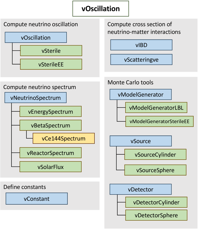
Figure 1: A simplified functional block diagram of the $\nu$Oscillation package, which includes calculations for the neutrino flux from nuclear reactors, the Sun, or from radioactive sources. It covers reactions such as IBD, beta decay, and neutrino-electron scattering. The package also implements neutrino mixing based on the PMNS matrix.

In order to validate the mixing effects implemented in the package $\nu$Oscillation, we reproduce an illustration of the neutrino oscillation in Ref. ref:nature_JUNO . It shows the flavour fractions as a function of the propagation distance when the neutrino energy is 4 MeV. We use the same oscillation parameters as in the Ref. ref:pars_PDG2014 , and the result is shown in Fig. 2. This confirms that our result is at least qualitatively consistent with the reference by comparing the locations of the bumps and the flavour fraction of the neutrinos.

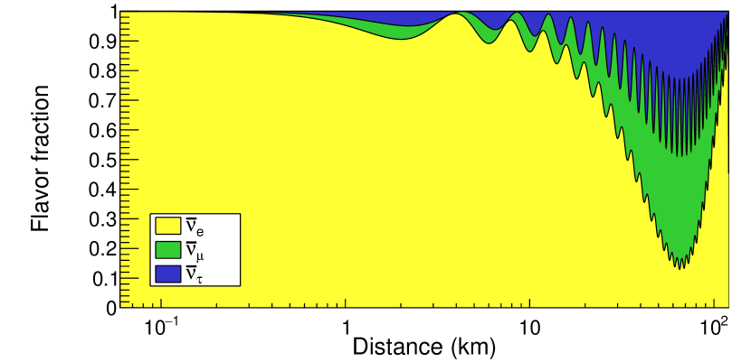
Figure 2: The fractions of each flavour as a function of distance computed by $\nu$Oscillation, are shown when there are $\bar{\nu}_{e}$ only in the initial state.

III Nuclear Reactor Neutrinos

The first step in computing the neutrino oscillation from nuclear reactors is to calculate the flux of anti-neutrinos produced by nuclear fission reactions within the reactors. For this calculation, we implement two models: the Huber-Mueller ref:Huber ; ref:Mueller and the Gutlein model ref:Gutlein in the vReactorSpectrum class. In the Gutlein model, the isotopes ²³⁵U, ²³⁸U, and ²³⁹Pu, are included, while the Huber-Mueller model includes ²⁴¹Pu in addition. This calculation requires input values of the relative abundance of each isotope and the thermonuclear power (in Watts we denote $\textrm{W}_{\textrm{th}}$) of a reactor. Using them as input information, the averaged differential neutrino flux at a distance $L$ from a nuclear reactor core is computed as

$$\Bigg{\langle}\frac{d\phi}{dE_{\bar{\nu}_{e}}}\Bigg{\rangle}=\frac{W_{\textrm{th}}}{\sum_{i}f_{i}E_{\textrm{re},i}}\frac{1}{4\pi L^{2}}\sum_{i}f_{i}\frac{d\phi_{i}}{dE_{\bar{\nu}_{e}}}$$ (3)

where $W_{\textrm{th}}$ is the thermal power of the reactor, $f_{i}$ is the fraction of a given fission isotope $i$, $E_{\textrm{re},i}$ is the thermal energy per fission, and $d\phi_{i}/dE_{\bar{\nu}_{e}}$ is the differential neutrino flux for the isotope $i$ at the nuclear reactor. For the detection of anti-neutrinos from a reactor, one has to consider two factors. First is the oscillation effect due to the neutrino mixing, and the second is the interaction of the anti-neutrinos in the detector, and for that one has to compute the event rate using the IBD cross section. Based on these, the detection probability can be expressed as

$$P^{\textrm{det}}_{\bar{\nu}_{e}\rightarrow\bar{\nu}_{e}}(L)=\frac{\int^{\infty}_{0}\langle\frac{d\phi}{dE_{\bar{\nu}_{e}}}\rangle\sigma(E_{\bar{\nu}_{e}})P_{\bar{\nu}_{e}\rightarrow\bar{\nu}_{e}}(L,E_{\bar{\nu}_{e}})dE_{\bar{\nu}_{e}}}{\int^{\infty}_{0}\langle\frac{d\phi}{dE_{\bar{\nu}_{e}}}\rangle\sigma(E_{\bar{\nu}_{e}})dE_{\bar{\nu}_{e}}}$$ (4)

where $\sigma(E_{\bar{\nu}_{e}})$ is the IBD cross section, and $P_{\bar{\nu}_{e}\rightarrow\bar{\nu}_{e}}(L)$ is the survival probability for electron anti-neutrino, respectively. Here we validate our computation to the existing nuclear reactor based experiment by reproducing a result in Ref. ref:nature_JUNO , and our result is shown in Fig. 3. The expected spectrum of the detected electron-antineutrinos is calculated by considering the reactor spectrum, the IBD cross section, and the neutrino oscillation with assuming a reactor located 53 km away from the detector. The energy resolution of 5% is assumed.

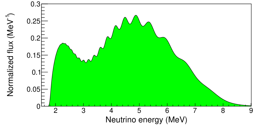
Figure 3: The expected spectrum of the detected electron-antineutrinos from a reactor located 53 km away from the detector is shown. The energy resolution of 5% is assumed.

For a case study with our $\nu$Oscillation, we choose an underground facility recently developed in Yemilab ref:Yemilab . This is an underground laboratory located at $37.2^{\circ}$ N, $128.7^{\circ}$ E in latitude and longitude of the Republic of Korea. A large hall, capable of hosting a 2 kton detector is located about 1000 m below the Yemi mountain. There are four nuclear reactors to be considered for the reactor anti-neutrino flux, and they are 65, 180, 216, and 282 km away with nuclear thermal power (name) of 20.8 (Hanul), 11.8 (Wolsong), 21.3 (Gori), and 16.9 (Hanbit) $\text{GW}_{\text{th}}$, respectively.

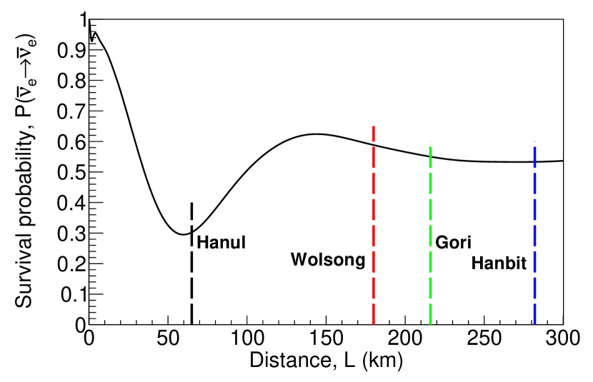
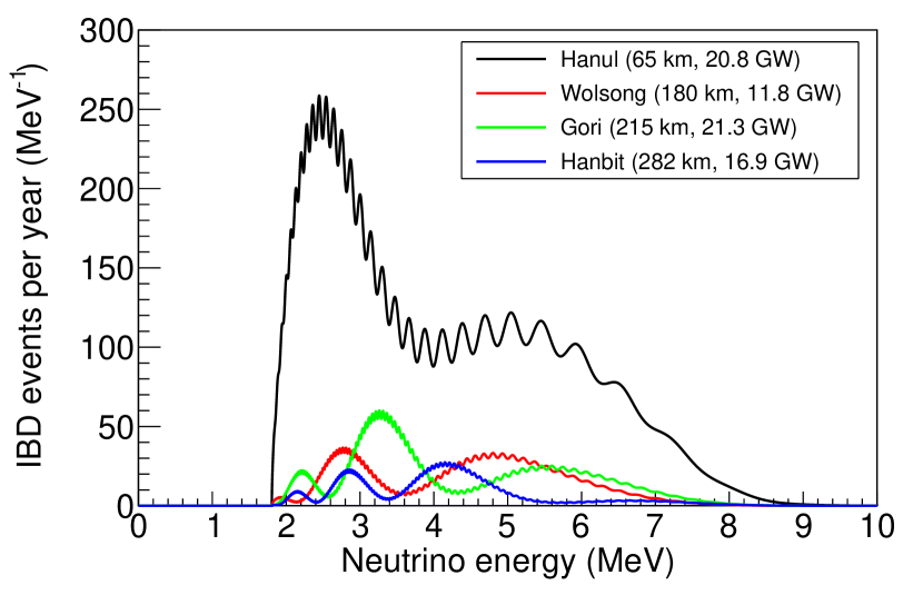
Figure 4: Top: our computation of the survival probability of anti-electron neutrino as a function of the distance from a nuclear reactor. The dashed lines indicate the location of the detector if a given reactor is at 0 km. Bottom: The expected IBD events from four nuclear reactors.

The distributions of IBD events as a function of distance and neutrino energy are shown in Fig. 4. Despite of having the lowest detection probability, the Hanul reactor is the dominant source of the IBD events as it is closest to the detector site. The estimated event rate of this source is approximately 860 events per year. In principle, with large statistics of data with excellent energy resolution, one can see the fine structure of a rapid oscillation due to $\theta_{13}$, but in practice, it will be limited by the volume of the detector and the energy resolution of the detector that originates from the photo-electron statistics.

IV Solar Neutrinos

The Sun is a natural source of electron neutrinos by nuclear fusion processes and by now so called the standard solar model ref:Bahcall describes the flux of electron neutrinos from various different fusion processes very precisely. In our study, we use parameters from the B16-GS98 model ref:Vinyoles to compute the solar neutrino flux. Solar neutrinos, arriving at detectors on Earth interact with detectors via neutrino-electron scattering. The differential yields of the scattering at different recoil kinetic energy ($T$) of the electron can be expressed as

$$\frac{dN_{e}}{dT} = n_{e}\int^{E_{\nu,\textrm{max}}}_{E_{\nu,\textrm{min}}}dE_{\nu}\frac{d\Phi}{dE_{\nu}}(E_{\nu})$$

$$\Bigg{(}\frac{d\sigma_{\nu_{e}}}{dT}(E_{\nu},T)P_{ee}+\frac{d\sigma_{\nu_{\mu},\nu_{\tau}}}{dT}(E_{\nu},T)(1-P_{ee})\Bigg{)}$$

(5)

where $n_{e}$ is the target electron number, $\frac{d\Phi}{dE_{\nu}}$ is the differential solar neutrino flux, $P_{ee}$ is the oscillation probability to the electron neutrino final state, $\frac{d\sigma_{\nu_{e}}}{dT}$ is the differential cross section of electron neutrino-electron ($\nu_{e}$-$e$) scattering ref:Bahcall_1995 , and $\frac{d\sigma_{\nu_{\mu},\nu_{\tau}}}{dT}$ is sum of the differential cross sections of $\nu_{\mu}$-$e$ and $\nu_{\tau}$-$e$ scattering.

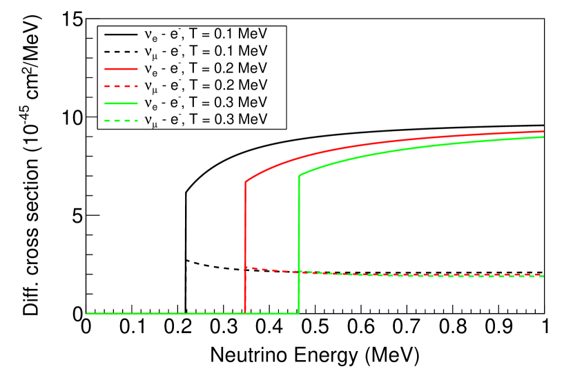
Figure 5: Neutrino-electron elastic scattering cross sections with different electron recoil energy values.

Figure 5 shows the implemented cross sections of neutrino-electron scatterings in Eq. (5) at different electron recoil energy values with different flavours of neutrinos. They are integrated with the solar neutrino flux model mentioned earlier in order to obtain spectra of scattered electron kinetic energy. Such spectra for $pp$, $pep$, CNO, ${}^{7}\textrm{Be}$, and ${}^{8}\textrm{B}$ neutrinos are shown in Fig. 6. The yield is normalized to the events per day per 1 keV per 100 ton of a liquid scintillator detector and the 5% energy resolution is assumed. The normalization and shapes are in general in agreement with results in Ref. ref:Borexino2021 . We also include two irreducible backgrounds. The first one is ${}^{14}\textrm{C}$ and is populated low end of the electron kinetic energy range. Here we assume the concentration of ${}^{14}\text{C}/^{12}\text{C}=1.94\times 10^{-18}$ ref:Borexino1998 . The second one is the so-called cosmogenic ${}^{11}\textrm{C}$ background that is sensitive to the depth of the site. Here we assume a site with 1000 m overburden. The ${}^{11}\text{C}$ neutrino spectrum differs in its shape from the reference spectrum ref:Borexino2021 because our result does not include detector responses such as the quenching as they are detector specific information.

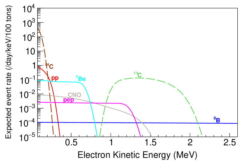
Figure 6: Expected electron kinetic energy distribution from various fusion processes in the Sun. The yield is normalized to the number per day per 1 keV per 100 tons of a detector. Also included two major irreducible backgrounds from ${}^{14}\textrm{C}$ and ${}^{11}\textrm{C}$.

V Sterile Neutrinos

Recently, several experiments indicate that the survival probability of electron neutrino in short range may be smaller than expected ref:LSND_anomaly ; ref:miniboone_anomaly ; ref:stereo_anomaly . This may originate due to the presence of a different type of neutrino, so-called sterile neutrino. We implement a (3+1) neutrino model in the $\nu$Oscillation, in which four mass eigenstates including one sterile neutrino, are mixed to construct three flavours.

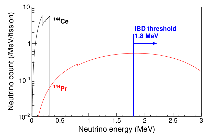
Figure 7: Energy distributions of neutrinos from $\beta^{-}$ decays of ${}^{144}\textrm{Ce}$ and ${}^{144}\textrm{Pr}$.

In order to estimate the sensitivity to the sterile neutrino search with the given radioactive source, we assume a radioactive source of ¹⁴⁴Ce with activity of 100 kCi as proposed earlier by other experiments ref:celand ; ref:dayabay ; ref:sox . The source is assumed to be located at the distance 9.5 m from the center of a cylindrical linear alkylbenzene (LAB) based liquid scintillator of 2 kton with a radius of 7.5 m. The ${}^{144}\textrm{Ce}$ decays to ${}^{144}\textrm{Pr}$ with the half life of 285 days, and ${}^{144}\textrm{Pr}$ decays to ${}^{144}\textrm{Nd}$ with the half life of 17 minutes, emitting $\bar{\nu}_{e}$. The energy distributions of anti-neutrinos from radioactive sources are shown in Fig. 7. Note that since the threshold for IBD is 1.8 MeV, only neutrinos from ${}^{144}\textrm{Pr}$ are sensitive to IBD. These spectra are implemented in $\nu$Oscillation accordingly.

Our likelihood for the binned data, $\bf n$, and given parameter set, $\Theta$, is defined as

$$\mathcal{L}(\Theta|{\bf n})=\prod_{i=1}^{N}\frac{m_{i}^{n_{i}}e^{-m_{i}}}{n_{i}!},$$ (6)

where $N$ is the number of bins, $n_{i}$ is the number of observed events in the $i$-th bin, and $m_{i}=m_{i}(\Theta)$ is the expected number of events from the model. Here, the binned data is in $L/E$, the ratio of the travel distance ($L$) of a neutrino to its energy ($E$). The model describes the expected distribution of neutrino events as a function of $L/E$. The parameter set, $\Theta=\{\sin^{2}2\theta_{14},\Delta m^{2}_{41}\}$, including the oscillation angle and the squared mass difference between the mass eigenstates 1 and 4, is commonly used to describe neutrino oscillation including sterile neutrino.

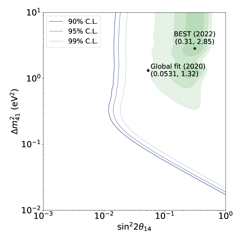
Figure 8: Exclusion sensitivity of the (3+1) neutrino model at 90%, 95%, and 99% confidence levels. A simulated data set of 34,000 IBD events without including sterile neutrino is compared with the (3+1) models. The one year of data taking and 70% detection efficiency are assumed. The best fit of global analysis of disappearance data and the BEST experiment are also marked, along with the $1$-$3\sigma$ confidence levels of the result of BEST indicated with green contours.

We simulate a data set without including the sterile neutrino oscillations. In total 34,000 neutrino events are generated by assuming the one year of data taking with 70% detection efficiency. The resolution for energy and position are not considered in this data. By comparing this data to the expected models with the sterile neutrino oscillations, we quantify the exclusion sensitivity at 90%, 95% and 99% confidence levels as shown in Fig. 8. The best fit of the global analysis of disappearance data ref:globalfit2020 and the result of the Baksan Experiment on Sterile Transitions (BEST) ref:best2022 are also marked.

VI Conclusions and Outlook

We developed a software package, $\nu$Oscillation, that calculates neutrino production and oscillation in nuclear reactors, neutrino-electron scattering from neutrinos originating from the Sun, and the oscillation of neutrinos originating from radioactive isotopes for the search of sterile neutrinos. Using our package, we discussed applications to the various neutrino experiments. We validated the package by reproducing the simulations on the neutrino spectra of reactor, solar and source neutrinos and the detection of them. We also verified the feasibility of this by calculating the sensitivity of a liquid scintillator detector to the sterile neutrinos. The current version of this software does not include the matter effect on the neutrino oscillation. This feature will be also implemented in the next release. This work is expected to be used in designs and optimizations of future neutrino experiments.

- (1) S. Weinberg, Phys. Rev. Lett. 19, 1264 (1967).
- (2) F. Englert and R. Brout, Phys. Rev. Lett. 13, 321 (1964).
- (3) P. W. Higgs, Phys. Rev. Lett. 13, 508 (1964).
- (4) G. S. Guralnik, C. R. Hagen, and T. W. B. Kibble, Phys. Rev. Lett. 13, 585 (1964).
- (5) D. J. Gross and F. Wilczek, Phys. Rev. Lett. 30, 1343 (1973).
- (6) H. D. Politzer, Phys. Rev. Lett. 30, 1346 (1973).
- (7) T. Kajita, E. Kearns, and M. Shiozawa, Nucl. Phys. B 908, 14 (2016).
- (8) Q. R. Ahmad et al. (SNO Collaboration), Phys. Rev. Lett. 87, 071301 (2001).
- (9) K. Eguchi et al. (KamLAND Collaboration), Phys. Rev. Lett. 90, 021802 (2003).
- (10) S. Pascoli and S. Petcov, Phys. Lett. B 544, 239 (2002).
- (11) K. Abe et al. (Hyper-Kamiokande Collaboration), Astrophys. J. 916, 15 (2021).
- (12) R. Acciarri et al. (The DUNE Collaboration), “Long-Baseline Neutrino Facility (LBNF) and Deep Underground Neutrino Experiment (DUNE) Conceptual Design Report Volume 1: The LBNF and DUNE Projects,” (2016), arXiv:1601.05471 [physics.ins-det].
- (13) M. Bustamante, “NuOscProbExact: a general-purpose code to compute exact two-flavor and three-flavor neutrino oscillation probabilities,” (2019), arXiv:1904.12391 [hep-ph].
- (14) C. A. Argüelles, J. Salvado, and C. N. Weaver, Comput. Phys. Commun. 277, 108346 (2022).
- (15) B. Pontecorvo, J. Exp. Theor. Phys. 7, 172 (1958).
- (16) C. Giganti, S. Lavignac, and M. Zito, Prog. Part. Nucl. Phys. 98, 1 (2018).
- (17) R. Brun and F. Rademakers, Nucl. Instrum. Methods. Phys. Res. A 389, 81 (1997).
- (18) F. L. Wilson, Am. J. Phys. 36, 1150 (1968).
- (19) P. Vogel and J. F. Beacom, Phys. Rev. D 60, 053003 (1999).
- (20) J. N. Bahcall, M. Kamionkowski, and A. Sirlin, Phys. Rev. D 51, 6146 (1995).
- (21) G. ’t Hooft, Phys. Lett. B 37, 195 (1971).
- (22) J. N. Bahcall, Rev. Mod. Phys. 59, 505 (1987).
- (23) P. Vogel, L. Wen, and C. Zhang, Nat. Commun. 6, 6935 (2015).
- (24) F. Capozzi, G. L. Fogli, E. Lisi, A. Marrone, D. Montanino, and A. Palazzo, Phys. Rev. D 89, 093018 (2014).
- (25) P. Huber, Phys. Rev. C 84, 024617 (2011).
- (26) T. A. Mueller, D. Lhuillier, M. Fallot, A. Letourneau, S. Cormon, M. Fechner, L. Giot, et al., Phys. Rev. C 83, 054615 (2011).
- (27) A. Gütlein, Doctoral dissertation, Technische Universität München (2013).
- (28) K. Park, J. Phys. Conf. Ser. 2156, 012171 (2021).
- (29) J. N. Bahcall, Phys. Rev. C 56, 3391 (1997).
- (30) N. Vinyoles, A. Serenelli, and F. L. Villante, J. Phys. Conf. Ser. 1056, 012058 (2018).
- (31) M. Agostini, K. Altenmüller, S. Appel, V. Atroshchenko, Z. Bagdasarian, D. Basilico, G. Bellini, J. Benziger, R. Biondi, and D. Bravo et al., Eur. Phys. J. C 81, 1075 (2021).
- (32) G. Alimonti et al. (Borexino Collaboration), Phys. Lett. B 422, 349 (1998).
- (33) A. Aguilar et al. (LSND Collaboration), Phys. Rev. D 64 112007 (2001).
- (34) A. A. Aguilar-Arevalo et al. (MiniBooNE Collaboration), Phys. Rev. Lett. 105, 181801 (2010).
- (35) H. Almazán et al. (The STEREO Collab oration), Nature 613, 257 (2023).
- (36) A. Gando, Y. Gando, S. Hayashida, H. Ikeda, K. Inoue, K. Ishidoshiro, H. Ishikawa, M. Koga, R. Matsuda, S. Matsuda, et al. (2014), arXiv:1312.0896 [phys.ins-det].
- (37) Y. Gao and D. Marfatia, Phys. Lett. B 723, 164 (2013).
- (38) G. Bellini et al. (Borexino Collaboration), “Sox: Short distance neutrino oscillations with borexino,” (2013), arXiv:1304.7721 [physics.ins-det].
- (39) A. Diaz, C. Argüelles, G. Collin, J. Conrad, and M. Shaevitz, Phys. Rep. 884, 1 (2020).
- (40) V. V. Barinov, B. T. Cleveland, S. N. Danshin, H. Ejiri, S. R. Elliott, D. Frekers, V. N. Gavrin, V. V. Gorbachev, D. S. Gorbunov, and W. C. Haxton et al., Phys. Rev. Lett. 128, 232501 (2022).