Common-Sense Bias Discovery and Mitigation for Classification Tasks

Abstract

Machine learning model bias can arise from dataset composition: sensitive features correlated to the learning target disturb the model’s decision rule and lead to performance differences along the features. Existing de-biasing work captures prominent and delicate image features which are traceable in model latent space, like colors of digits or background of animals. However, using the latent space is not sufficient to understand all dataset feature correlations. In this work, we propose a framework to extract feature clusters in a dataset based on image descriptions, allowing us to capture both subtle and coarse features of the images. The feature co-occurrence pattern is formulated and correlation is measured, utilizing a human-in-the-loop for examination. The analyzed features and correlations are human-interpretable, so we name the method Common-Sense Bias Discovery (CSBD). Having exposed sensitive correlations in a dataset, we demonstrate that downstream model bias can be mitigated by adjusting image sampling weights, without requiring a sensitive group label supervision. Experiments show that our method discovers novel biases on multiple classification tasks for two benchmark image datasets, and the intervention outperforms state-of-the-art unsupervised bias mitigation methods.

1 Introduction

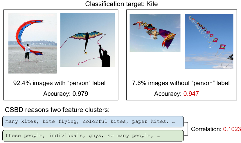
Figure 1: Sensitive features are everywhere: Small objects which co-occur frequently with the target can affect model prediction, for example, kites and people in MS-COCO images. Sensitive features like this are of multiple types and may cause different downstream biases. Our method aims to discover comprehensive sensitive correlations in a dataset based on common-sense descriptions, and treat biases which have not been explored in literature.

Computer vision has been deployed with dramatically more diverse data (both realistic and generative) in recent years, which has drawn attention to the inherent bias in a lot of datasets [54]. One common bias is due to the co-occurrence of target features with auxiliary context or background features (illustrated in Figure 1), which models may rely on in making predictions even though the relationship is not robust and generalizable [50, 27, 7]. Current bias detection algorithms have diagnosed such co-occurrences from model encoded representations, based on the representations’ varied sensitivity to different auxiliary features [28, 6, 52, 60].

However, these methods rely on image-based embeddings and thus are limited to only identifying certain kinds of bias that could be captured in that embedding space. For example, previous studies have shown that visual features that occupy smaller spatial area can lead to worse representations [55]. Therefore, subtle facial features such as eyeglasses frames or small object features like a keyboard nearby a cat can be overlooked for bias modeling. These observations suggest that modeling with additional data modalities, specifically text descriptions of images, may be beneficial in bridging this gap. Such an approach of “common-sense reasoning” by natural language [24, 5, 44, 13] allows high-level abstract understanding of images and reasoning for subtle image features, thus can facilitate better dataset diagnosis and bias discovery than relying on the image modality alone.

There have been some early explorations in this direction. For example, given that text embedding is a good proxy to image embedding in representation space [67], auxiliary features to the target such as ocean and forest for waterbird recognition are expressed as text sets. Each text-based feature is encoded and aligned to the model’s inner state to measure the feature’s influence [60, 67]. However, the use cases of the existing common-sense bias modelings are limited in two major aspects: First, though text-based features can be more diverse than traditional image-based patterns, they are limited by the prior knowledge of the humans writing them and cannot expose unlabeled or subtle features in a dataset. Second, the additional step of embedding space alignment using models like CLIP [44] or generative models [46] lacks the ability to control fine-grained image regions with text, and may inherit extra bias from the models [8, 47].

To bridge the gap, we propose a novel method of description-based reasoning for feature distribution and potential model bias called Common Sense Bias Discovery (CSBD), shown in Figure 2. Taking a description corpus of images (for example, descriptive captions), we unpack it into a hierarchy of “categories” (major subjects in an image) and subordinate “features” (different attributes or states of a subject) via text embedding clustering. The features are extracted from descriptions’ semantic components so they represent image content comprehensively, not limited by prior knowledge or cross-modal alignment. Then, correlations between features are quantified based on their occurrence across all data samples. It should note that discovered correlated features are not necessarily bias: for example, a correlation between “teeth” and “smile” in a dataset of face images is both expected and entirely benign. Therefore, we maintain a human-in-the-loop component in our pipeline to identify sensitive/spurious correlations. However, after the identification step, our method does not need a human-in-the-loop to treat the potential bias these correlations might cause. We summarize our contributions as follows:

1. A novel common-sense reasoning approach that discovers human-interpretable “feature clusters” (beyond the image embedding level) existing in image datasets.

2. Based on the clusters, a formulation to derive pairwise image feature correlations, order them by significance, and allow human domain experts to identify sensitive correlations for further intervention.

3. Empirical evidence that our method discovers subtle sensitive features and model biases for classification tasks, which to the best our knowledge has not been previously identified and addressed. Furthermore, we adjust data sampling weights calculated by our method and achieve state-of-the-art results bias mitigation results.

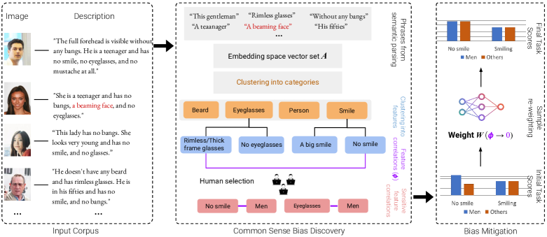
Figure 2: Common Sense Bias Discovery (CSBD) system and the mitigation strategy overview: Given the input corpus of image and corresponding description pairs (Left), the descriptions are parsed into semantically meaningful phrases and encoded into embedding space vectors. A two-stage clustering on the vector set generates a list of common-sense feature clusters. Then, correlations between every two feature distributions are computed and highly-correlated features are examined by a human for mitigation (Middle). Finally, correlations are mitigated by adjusting image sampling weights during training, calculated automatically from the derived feature distributions (Right).

2 Related Works

2.1 Bias discovery

Unsupervised bias discovery.

Many recent studies have focused on waiving the need for sensitive group annotation to achieve model robustness between groups. One approach is to assume that easy-to-learn data samples lead to learning shortcut attributes, thus resulting in biased classifiers. These bias-aligning samples are identified based on higher prediction correctness and confidence [22, 32, 65], gradient [1], or being fitted early in training [39]. Feature clustering has also been used, leveraging the observation that samples with same attributes are located closely in feature space, and thus bias is inferred from the trained model’s unequal performance between clusters  [48, 23]. Other approaches model attributes as latent variables and identify influential attributes by latent space distribution of training samples [4, 25], or find subsets of samples which have maximum predicted probabilities on a target to indicate a biased group  [30]. However, the implicit bias supervision used in these methods lacks transparency, and the ways of inferring discounted samples or latent variables during training might not be robust to training algorithm or schedule shifts. Our method depends on data description reasoning for bias discovery thus is generalizable to different training targets and schemes.

Bias mitigation.

Methods that discover bias-aligned samples or clusters use them as a supervision to upweight low performers and thus train a debiased model [39, 23, 32, 1, 48], or encourage the model to learn similar representations for samples with same target label but different sensitive attributes via contrastive learning [65, 40, 63]. Augmentation is also used on bias-aligned images to translate the style while maintaining the target content [22, 45]. Real-time bias mitigation can be done adaptively with bias identification to inspect learnt latent features throughout training, including penalizing the classifier for violations of the Equal Opportunity fairness criterion [30] or to update latent variables of a variational autoencoder that debiasing is based on [4, 3]. Though these frameworks all use end-to-end interventions to tackle unwanted model behaviors, the discovered bias is not tangible and is dependant on the learning protocols. Therefore, the mitigation methods lack the flexibility to treat different bias types rooted in data, in contrast to our method.

2.2 Text-Image methods

Visual-semantic Grounding.

To ground representations of images with natural linguistic expression, models learn an embedding space where semantically similar textual and visual features are well aligned [20, 59, 17, 44]. Such models can be extended to align representations from local image regions, and can adapt to various multi-modal tasks  [62, 2, 64, 68]. They motivate new downstream applications via “prompting”; examples include domain adaptation by augmenting image embeddings prompted by target domain text descriptions [14], aligning positional features of animals’ pose estimation using pose-specific text prompts [66], and conditional image synthesis by training token generators for knowledge transfer [51]. Unlike other methods that leverage multi-modal embedding spaces to intervene model training, our analysis and intervention are data-focused for balancing feature distribution. Therefore, while prompts usually need to be handcrafted or fine-tuned with alternate learning structures [21, 51], our method handles text inputs with arbitrary content without an additional training heuristic.

Bias discovery with cognitive knowledge.

Building machine learning systems with cognitive ingredients based on human judgement is a widely-discussed topic [24, 57]. It introduces domain expertise to improve model performance with minimal cost [61]. For bias discovery purposes, “frequent item sets” is analyzed in visual question answering (VQA) dataset and association rules are discovered to interpret model behaviors [35]. Human is also included to look at a traversal of synthesized images along attribute variations, and interpret the attribute’s semantic meaning [29]. Wu et al. [60] build a collection of human-interpretable visual patterns like stripes and test their correlations to image samples. Zhang et al. [67] design language prompts to generate counterfactual samples and identify influential attributes. However, such methods are limited by an empirical feature set which the model prediction bias is analyzed with. The human defined features may not generalize to different image domains, thus, we use clustering and correlation analysis for any datasets with an uncurated description corpus.

3 Method

In this section, we propose a novel Common-Sense Bias Discovery method, referred to as CSBD. Given a corpus of (image, text description) pairs, our method analyzes pairwise feature correlations based on common-sense text descriptions. This is followed by a human-in-the-loop step, where a domain expert reviews the identified correlations and selects the ones that may negatively impact the downstream classification task. Finally, based on the selected correlations, we mitigate model bias via a simple data re-weighting strategy, without a requirement for sensitive group labels. The method is illustrated in Figure 2, with algorithm steps detailed in Algorithm 1, and the major components are described below.

Language-inferred feature distribution.

The natural language image descriptions must first be broken down to align with local visual features. We use SceneGraphParser [59] on the text descriptions to split the sentences and extract spans of noun phrases as semantic rich components, e.g. split “The girl has a big smile” into “The girl” and “a big smile”. $M$ denotes the the total number of parsed phrases in a dataset. We then use a pre-trained model, Universal Sentence Encoder (USE) [10], to encode the phrases into embedding vectors; this model is trained to extract sentence-level embeddings, and performed better than other language models such as CLIP in our experiments (Sec. 5). Phrase vector dimensions are reduced to dimension $d$ (tuneable hyper-parameter) using PCA [19] before being clustered.

Next, we implement a two stage clustering process, using the K-means clustering algorithm [34] for both stages: (1) All phrase embedding vectors $\boldsymbol{A}\in\mathbb{R}^{d}$ are clustered into $C$ categories, where $C$ is a tunable hyper-parameter (datasets including more diverse categories of objects should have a larger $C$); (2) Each category cluster $c$ is further clustered into $F_{c}$ features, e.g., if the cluster is for Smile category and $F_{c}=3$, example features could be “a mild smile”, “no smile”, and “beaming smile”. The value of $F_{c}$ is determined on a per-cluster basis as follows: we set a pre-defined upper bound ${\sigma}_{max}$, and for each category cluster $c$ we take $F_{c}$ to be the smallest integer such that the mean within-cluster variance of the features is lower than $\sigma_{max}$. The within-cluster variance of a feature is given by the sum of the squared distance between the centroid point and each point of the cluster; this is the standard measure of spread used in K-means clustering. Using the variance instead of a fixed number of clusters for the second clustering allows each category to contain different number of features; this is important because some categories can have a natural binary split (e.g. eyeglasses/no eyeglasses) while others may have a much wider range of features (e.g. age groups). As a result, we obtain a hierarchy of visual feature descriptions that comprehensively cover the dataset and are consistent with common-sense descriptions.

Input: Image corpus $G=\{g_{1},g_{2},...,g_{N}\}$.

   Description corpus $D=\{d_{1},d_{2},...,d_{N}\}$

Parsing and encoding:

 $D\rightarrow P=\{p_{1},p_{2},...,p_{M}\}$   $\triangleright$ $P$ is the phrase set

 $\boldsymbol{A}=e(P)=\{\boldsymbol{p}_{1},\boldsymbol{p}_{2},...,\boldsymbol{p}_{M}\}\in\mathbb{R}^{M\times 512}$

          $\triangleright$ $e$ is a pre-trained text encoder

Clustering:

 $\boldsymbol{A}\rightarrow C\text{ sets }\{\boldsymbol{S}_{1},...,\boldsymbol{S}_{C}\}$     $\triangleright$ Vector cluster

 $A\rightarrow\{S_{1},...,S_{C}\}$  $\triangleright$ Natural language phrase cluster

 for $c$ from $1$ to $C$ do:

  $\boldsymbol{S_{c}}\rightarrow F_{c}\text{ sets }\{\boldsymbol{B}_{1},...,\boldsymbol{B}_{F_{c}}\}$, s.t. $\text{Var }\boldsymbol{B}_{i}\leq{\sigma}_{max}$

  $S_{c}\rightarrow\{B_{1},...,B_{F_{c}}\}$

 $F=F_{1}+F_{2}+..+F_{C}$ $\triangleright$ Number of feature clusters

Computing correlation:

 for $f$ from $1$ to $F$ do:

  $\boldsymbol{t}_{f}=\{t_{1},t_{2},...,t_{N}\}$  $\triangleright$ Feature one-hot indicator

  , where $t_{i}=1$ , if $\exists\text{\break}p\in B_{f}$: $p$ in $d_{i}$, else $t_{i}=0$

 for $f$ from $1$ to $F$ do:

  for $f^{\prime}$ from $1$ to $F$, $f^{\prime}\neq f$ do:

   $\boldsymbol{t}_{f},\boldsymbol{t}_{f^{\prime}}\rightarrow\phi_{\boldsymbol{t}_{f}\boldsymbol{t}_{f^{\prime}}}$   $\triangleright$ phi correlation coefficient

Outputs: $[B_{f},B_{f^{\prime}}]$ , for $f,f^{\prime}$ where $\lvert\phi_{\boldsymbol{t}_{f}\boldsymbol{t}_{f^{\prime}}}\lvert>z$

Algorithm 1 CSBD. $N$ is the size of the dataset. $M$ is the number of parsed phrases. $C$ is the number of category clusters. ${\sigma}_{max}$ is the upper bound of within-cluster variance. $z$ is the threshold of feature correlation coefficient.

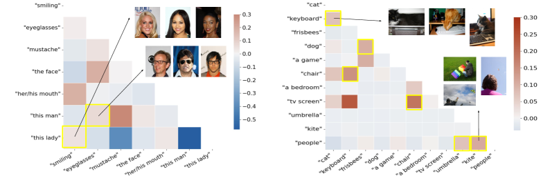
Figure 3: Examples of discovered correlations in CelebA (Left) and MS-COCO (Right) dataset, and the correlation coefficients. Sensitive correlations are circled in yellow, such as “the lady” and “smiling”. The others are viewed as benign, like “man” and “mustache”.

Discovering feature correlations.

Having extracted a set of feature clusters in the previous step, the next step is understanding feature co-occurence within the dataset. This allows us to identify spurious correlations relevant to the target task, which may cause model bias. To quantify such correlations: first, we generate a one-hot indicator for each feature: $\boldsymbol{t}_{f}=[t_{1},t_{2},...,t_{N}]$, where $N$ is the size of the dataset, and $t_{i}=1$ if the $f^{th}$ feature occurs in the $i^{th}$ image’s description, otherwise $t_{i}=0$. Second, the phi coefficient $\phi$ [12, p. 282] is used to measure the association between every two indicators. The phi coefficient between two indicators $\boldsymbol{t}_{f}$ and $\boldsymbol{t}_{f^{\prime}}$ is defined as follows:

$$\small\phi_{\boldsymbol{t}_{f}\boldsymbol{t}_{f^{\prime}}}=\frac{x_{11}x_{00}-x_{10}x_{01}}{\sqrt{x_{1*}x_{0*}x_{*0}x_{*1}}},$$ (1)

where $c\in[0,C)$, $f,f^{\prime}\in[0,F_{c}]$, and

$$\small x_{11}=\|\boldsymbol{t}_{f}\cdot\boldsymbol{t}_{f^{\prime}}\|_{1},\quad x_{01}=\|(\neg\boldsymbol{t}_{f})\cdot\boldsymbol{t}_{f^{\prime}}\|_{1},$$

$$\small x_{10}=\|\boldsymbol{t}_{f}\cdot(\neg\boldsymbol{t}_{f^{\prime}})\|_{1},\quad x_{00}=\|(\neg\boldsymbol{t}_{f})\cdot(\neg\boldsymbol{t}_{f^{\prime}})\|_{1},$$

$$\small x_{1*}=\|\boldsymbol{t}_{f}\|_{1},\quad x_{0*}=\|\neg\boldsymbol{t}_{f}\|_{1},$$

$$\small x_{*0}=\|\neg\boldsymbol{t}_{f^{\prime}}\|_{1},\quad x_{*1}=\|\boldsymbol{t}_{f^{\prime}}\|_{1}.$$

$\neg$ denotes element-wise negation, $\|\cdot\|_{1}$ denotes the $L^{1}$ norm.

Two features are positively correlated (likely to co-occur in an image) if $\phi$ is a positive value, and are negatively correlated (rarely co-occur) if $\phi$ is a negative value. A $\phi$ near zero indicates two features which co-occur randomly.

Intuitively, features that have high correlation with any target features can become shortcuts for model learning and cause biased decision-making toward certain subgroups [53, 9]. Thus feature pairs which have $\lvert\phi\rvert>z$ (where $z$ is an empirically decided threshold and can be adjusted) are returned for examination by a human. The human has access to the common-sense text descriptions of each feature. In most cases, the returned feature pairs are naturally connected (e.g. “teeth visible” with “a smile”, and most facial features with “the face”). These correlations are usually robust and generalizable, and thus viewed as benign. The benign correlations usually exist, besides, the function of feature correlations vary across different downstream learning scenarios and not all correlations need to be treated. Therefore, a human-in-the-loop step is necessary to ensure that only sensitive correlations that may affect the target task are selected. The human-in-the-loop component of our pipeline, like previous efforts [35, 29, 60, 67], allows flexibility and transparency for bias mitigation.

Bias mitigation via re-weighting.

Enhancing model learning of discounted samples is a common bias reduction approach  [1, 49, 58]. Therefore, to simplify the intervention needed for correcting biases surfaced by our method, we follow the previous work in [1] to adjust data sampling weights.

Specifically: given a set of targets and human-identified sensitive features correlated to them, the goal is to balance the distribution of samples with vs. without each sensitive feature across the targets. That is, if the downstream task is smile detection then images with, say, the “man” feature and without the feature should have the same ratio of positive to negative target labels. This condition ensures a statistical independence between each feature and target [42].

The new data sampling weights are calculated as follows. We denote the dataset as $D$, target set as $Y$, target feature indicators obtained from the last step as $\boldsymbol{t}_{Y}=\{\boldsymbol{t}_{y}:y\in Y\}$, and the sensitive features indicator as $\boldsymbol{t}_{s}$. Further, we denote the original feature distribution with respect to the targets as $P_{D}(\boldsymbol{t}_{s}|\boldsymbol{t}_{Y})$ and $P_{D}(\neg\boldsymbol{t}_{s}|\boldsymbol{t}_{Y})$, with $P$ representing probability. The sampling weight $W(\boldsymbol{t}_{s}|\boldsymbol{t}_{Y})$ for images with feature $s$ across the targets is defined by the following equation:

$$P_{D}(\boldsymbol{t}_{s}|\boldsymbol{t}_{Y})\cdot W(\boldsymbol{t}_{s}|\boldsymbol{t}_{Y})=P_{D}(\neg\boldsymbol{t}_{s}|\boldsymbol{t}_{Y})$$ (2)

In the ideal case where the dataset target feature distribution is already balanced w.r.t the sensitive feature, the sampling weight $W(\boldsymbol{t}_{s}|\boldsymbol{t}_{Y})$ would be equal to 1. The intervention is to treat one sensitive feature $s$ and model bias it causes.

Finally, we also implement randomized augmentations alongside the sampling weights to introduce data diversity.

4 Experiments

	Vanilla (no mitigation)		LfF [39]		DebiAN [30]		PGD [1]		BPA [48]		CSBD (ours)
Target	Worst ($\uparrow$)	Avg. ($\uparrow$)	Worst ($\uparrow$)	Avg. ($\uparrow$)	Worst ($\uparrow$)	Avg.($\uparrow$)	Worst($\uparrow$)	Avg. ($\uparrow$)	Worst ($\uparrow$)	Avg. ($\uparrow$)	Worst ($\uparrow$)	Avg.($\uparrow$)
Smiling	0.894 (3e-3)	0.919 (2e-3)	0.730 (0.03)	0.841 (7e-3)	0.895 (0.01)	0.916 (7e-3)	0.888 (0.02)	0.917 (1e-3)	0.899 (3e-3)	0.912 (6e-3)	0.908 (3e-3)	0.918 (9e-4)
Eyeglasses	0.926 (3e-4)	0.964 (2e-3)	0.810 (0.02)	0.911 (7e-3)	0.928 (0.01)	0.964 (6e-3)	0.917 (8e-3)	0.960 (3e-3)	0.929 (5e-3)	0.962 (2e-3)	0.938 (2e-3)	0.965 (1e-3)

Table 1: Treating common-sense bias discovered by CSBD towards the target ground truth label (Target): (1) “Smiling” and (2) “Eyeglasses”, among the sensitive group label: “Male” and others, on CelebA dataset. The average classification accuracy of all target-sensitive groups (Avg.), and the worst performing group (Worst), are reported. Results are based on three independent runs and standard deviation is given in parenthesis. The best results are marked in bold and the second best results are underlined. Group-level results are in the Supplementary.

		Vanilla (no mitigation)		LfF [39]		DebiAN [30]		PGD [1]		BPA [48]		CSBD (ours)
Target	Sensitive	Worst($\uparrow$)	Avg. ($\uparrow$)	Worst ($\uparrow$)	Avg. ($\uparrow$)	Worst ($\uparrow$)	Avg. ($\uparrow$)	Worst ($\uparrow$)	Avg. ($\uparrow$)	Worst ($\uparrow$)	Avg. ($\uparrow$)	Worst ($\uparrow$)	Avg. ($\uparrow$)
Cat	Couch	0.849 (0.04)	0.935 (8e-3)	0.800 (0.04)	0.916 (0.01)	0.821 (0.01)	0.902 (9e-3)	0.884 (9e-3)	0.940 (3e-3)	0.853 (0.03)	0.925 (5e-3)	0.906 (4e-3)	0.941 (3e-3)
Cat	Keyboard	0.948 (1e-3)	0.972 (6e-3)	0.870 (0.04)	0.938 (9e-3)	0.917 (4e-3)	0.949 (2e-3)	0.947 (7e-4)	0.977 (2e-4)	0.890 (0.05)	0.952 (0.02	0.953 (1e-3)	0.976 (6e-4)
Dog	Frisbee	0.883 (9e-3)	0.927 (6e-3)	0.821 (0.04)	0.893 (0.02)	0.845 (0.02)	0.895 (2e-3)	0.872 (6e-3)	0.940 (4e-3)	0.854 (0.02)	0.905 8e-3)	0.903 (5e-3)	0.934 (5e-3)
TV	Chair	0.726 (8e-3)	0.893 (2e-3)	0.690 (0.02)	0.867 (6e-3)	0.718 (0.01)	0.876 (3e-3)	0.821 (7e-3)	0.907 (2e-3)	0.758 (0.02)	0.887 (5e-3)	0.842 (7e-3)	0.911 (1e-3)
Umbrella	Person	0.761 (0.01)	0.880 (2e-3)	0.771 (4e-3)	0.854 (5e-3)	0.716 (0.04)	0.857 (0.01)	0.763 (0.01)	0.887 (2e-3)	0.777 (0.02)	0.878 (8e-3)	0.814 (9e-3)	0.892 (1e-3)
Kite	Person	0.937 (0)	0.963 (4e-4)	0.854 (0.02)	0.923 (7e-3)	0.941 (0.02)	0.960 (6e-3)	0.917 (0)	0.955 (1e-3)	0.921 (6e-3)	0.957 (2e-3)	0.945 (7e-3)	0.960 (3e-3)

Table 2: Treating common-sense bias discovered by CSBD between each target ground truth label (Target) and sensitive group label (Sensitive), for binary object classification task on MS-COCO dataset. The average classification accuracy of all target-sensitive groups (Avg.), and the worst performing group (Worst), resulted from feature correlations, are reported.

We conduct downstream experiments to answer: (1) Do the sensitively correlated features reasoned by CSBD align with model bias on popular benchmark datasets? (2) Can prior correlation-robust methods prevent such bias? (3) Is the reasoned bias curable using simple data-wise intervention?

4.1 Datasets

CelebA-Dialog

[18] is a visual-language dataset including captions for images in CelebA [33], a popular face recognition benchmark dataset containing 40 facial attributes. Each caption describes 5 fine-grained attributes: “Bangs”, “Eyeglasses”, “Beard”, “Smiling”, and “Age”. Since the captions are generated as natural language sentences, they also include other common-sense information like pronouns and people titles (phrases like “the man” or “the lady”). Since we are limited to the facial features each caption describes, our analysis will not pick up the well-known correlations, such as “HairColor” and “HeavyMakeUp”, studied in prior work [39, 65, 1]; however, we instead identify new correlations not found by other methods (see Sec. 4.3.1). For classification tasks, we select the target labels as “Smiling” and “Eyeglasses”, and the sensitive group label to be “Male” (here “label” refers to the ground truth binary labels). The labels are selected because their corresponding caption-inferred features are discovered by our method to be highly correlated and thus may cause downstream model bias.

MS-COCO 2014

[31] is a large-scale scene image datasets including annotations for 80 objects, and each image has 5 descriptive captions generated independently [11]. We randomly select 1 caption for each image. Based on our feature correlation analysis, we select 7 target and sensitive label pairs for training downstream models and evaluating bias, as listed in Table 2. For example, we train a model for recognizing “Dog” and evaluate if the model shows performance disparity for images with/without “Frisbee”. We perform binary classification on each target label, following  [56]. This is because although MS-COCO is more used for multi-label classification, certain labels will need to be treated as auxiliary features in order to reveal their effects on the target and thus study bias caused by feature correlations.

4.2 Implementation

For correlation reasoning, the phrases from the description corpus are encoded to vectors in 512 dimensions using Universal Sentence Encoder (USE). The dimension is reduced using PCA to 30 for the CelebA dataset and 100 for MS-COCO, which ensure that the sum of the PCA components’ explained variance was over 90%. The embedding vectors are then scaled to unit norm before being clustered using K-means. We set the category cluster number $C$ to 8 for CelebA and 50 for MS-COCO. These numbers are empirically selected to ensure no obvious discrepancies in discovered clusters: that is, no redundant clusters or multiple categories in same clusters. For the second step which generates feature clusters, the upper bound of the within-cluster variance $\sigma_{max}$ is set to 0.15 for CelebA and 0.5 for MS-COCO; see Sec. 5 for sensitivity analysis. The threshold $z$ for correlation coefficient between two feature indicators is chosen to be 0.05 (correlation significance is verified by Chi-square test [41]). Empirically, feature correlations higher than $z$ cause bias on the datasets we used.

For the downstream training, we use the same training, validation, and testing split as in [65] for the CelebA dataset, as in [38] on the MS-COCO dataset. However, because of label scarcity of individual objects relative to the entire dataset (for example, only 3% of images in MS-COCO contain “Cat” and 2% of images contain “Kite”), to avoid class imbalance problem introducing confounding bias to the classifier, we randomly take subsets of the dataset splits which include 50% of each target label. Further implementation details are given in the Supplementary.

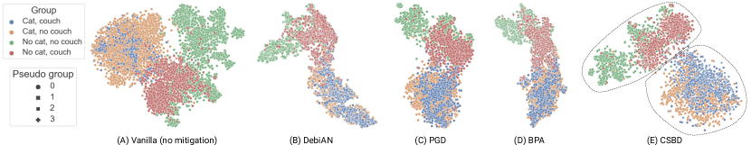
Figure 4: T-SNE results for cat classifiers (“Couch” as sensitive label) trained with MS-COCO dataset. Target attributes (“Cat” $\bullet$ $\bullet$ and “No cat” $\bullet$ $\bullet$) are most linearly separable with CSBD-trained embeddings (E) compared to the baseline and other bias mitigation methods (A-D). Methods which can discover pseudo sensitive groups are marked with group assignment by $\bullet$ and $\times$. Comparing to the real groups (“Couch” $\bullet$ $\bullet$ and “No couch” $\bullet$ $\bullet$) across which bias is expected to be treated, CSBD obtains the closest estimation.

4.3 Results

4.3.1 Correlation discovery results

CelebA.

Semantic parsing of the image descriptions generates $M=1,\!283,\!552$ phrases for CelebA dataset, and applying CSBD outputs 72 feature pairs that have an absolute correlation coefficient higher than $z=0.05$. By manual check, we determine that the features “smiling” and “eyeglasses” are both sensitively correlated to people-title features “the man, the guy, ...” and “the lady, the girl, ...”, and we designate other naturally related features like “mouth” and “smiling” as benign. The correlation values between sensitive features, along with selected benign correlations, are visualized in Figure 3 (Left), and the full list is in the Supplementary.

MS-COCO.

Semantic parsing for descriptions generates $M=253,\!467$ phrases. CSBD outputs 220 correlated feature pairs for the MS-COCO dataset. The benign examples include “frisbee” and “a game”, “waves” and “ocean”, etc. The sensitive ones include “cat” and “couch”, “kite” and “people”; see Table 2 for the 7 examples chosen for bias mitigation, and the full list is given in the Supplementary. Although these connections are intuitive, models can learn and utilize the feature dependence: for example, recognition of a kite in an image may not be based on its shape but whether it co-occurs with people. Selected results are visualized in Figure 3 (Right).

4.3.2 Bias mitigation results

To verify whether the spurious feature correlations discovered by CSBD can indicate and help mitigate downstream model bias, we report image classification results on CelebA and MS-COCO dataset in Table 1 and Table 2. We use the worst group performance to evaluate model bias, following [65, 1, 48], and the groups are all combinations of target label and sensitive feature label pairs as in [65]. Baseline model without bias mitigation (Vanilla) for all tasks presents a gap between the worst-performing group (Worst) and the group average (Avg.), indicating the classifier’s bias. For example, images containing Chair but no TV obtain an accuracy of 0.726, 19% lower than the average accuracy (Table 2). CSBD re-weights sampling probabilities to break the correlations in the dataset, using the reweighting factor given in equation (2). We see from Tables 1 and 2 that CSBD successfully mitigates model bias (most improved Worst Group Performance) on all targets, outperforming the baseline and other de-biasing methods: LfF [39], DebiAN [30], PGD [1], and BPA [48]. Moreover, model classification quality will not be degraded by using our method: CSBD always obtains the highest or the second highest average group accuracy.

4.4 Discussion

We investigate the advantage of our method over other unsupervised bias mitigation methods by discussing the common-sense bias’s differentiation to embedding-based bias, specifically, how bias affects model predictions and the treatment required. We visualize image embeddings extracted from the fully connected layer of the “Cat” classification models trained with MS-COCO. Model bias can be observed from the vanilla baseline with no intervention (Figure 4 (A)): while target classes are separable for samples without sensitive feature (orange and green dots), for images with sensitive feature the model’s prediction boundary for the target is blurred (blue and red dots are partially mixed).

This is different to the specific bias types our comparison methods study, that sensitive features are easily distinguishable in embedding space. LfF [39] assumes that the biased model presents an unintended decision rule to classify sensitive features, which appear in images aligning with the decision rule. However, this unintended decision rule does not generate in the biased model training (Figure 4 (A)). DebiAN assigns pseudo sensitive groups as two sample splits which get unequal positive prediction rates [30], which cannot capture meaningful feature (Figure 4 (B)). BPA clusters embeddings and assume different clusters represent different sensitive features [48]. However, embeddings of samples with/without couch feature are not separable and the method only discovers target-related clusters (Figure 4 (D)). PGD does not split pseudo groups but identifies bias conflicting samples by model-computed gradient [1]. Re-weighting based on gradients does not correct the decision boundary (Figure 4 (C)), indicating that samples with the sensitive feature that cause bias are not precisely identified. In sum, for common-sense bias caused by the sensitive features not pronounced in image embeddings, methods which rely only on image will show ineffective bias discovery and mitigation.

In contrast, text-based reasoning provides high-level abstract understanding of the image itself, regardless of how model parameters or embeddings encode the image. Such understanding discovers sensitive features correlated to the target, including “a couch”, precisely. Our method removes the correlation from dataset and trains a model with much clearer decision boundary for “Cat”, not affected by presence of “Couch” (Figure 4 (E)). Though the reasoning is not based on true feature labels but coarse descriptions with incomplete information (which explains why not all “Couch” samples are classified in a group), it can still quantify data feature imbalance and lead to effective bias mitigation.

There are other benchmark datasets for bias studies including colored MNIST [26], corrupted CIFAR [16], etc. We don not include these datasets because the biases are limited by single feature type (like color), or low-level image properties like brightness and contrast, not in the scope of reasoning features by common-sense knowledge.

5 Ablation

Text-based embedding encoder.

In the language-inferred feature distribution step, we use the Universal Sentence Encoder (USE) [10] which is trained and optimized for sentence level text data. Here we test with a different language model, namely the text encoder of CLIP, which is a modified form of the GPT-2 architecture [43]. The encoder is used to extract phrase embeddings, and clustering is performed as described in Algorithm 1 to generates 8 category clusters on the CelebA dataset. To compare how well different text encoder embeddings retain semantic information to produce reasonable clusters, we compute the mean within-cluster variance of generated clusters. The variance using CLIP text encoder embeddings is 0.4735, while the variance using USE embeddings is 0.3531. Therefore, USE is the better text encoder with respect to clustering common-sense phrases.

Dimension reduction algorithm.

We experiment with changing the linear dimension reduction technique from PCA [19] to UMAP [37], which can reflect nonlinear structure from the original embedding space to more than 2 dimensions. Embedding dimension is reduced to 30 to perform clustering as in Sec. 4.2. The mean within-cluster variance of generated category clusters on the CelebA dataset increases from 0.3531 to 0.3916 when using UMAP, which indicates that the linear dimension reduction PCA applied on embeddings produces better clustering for this application.

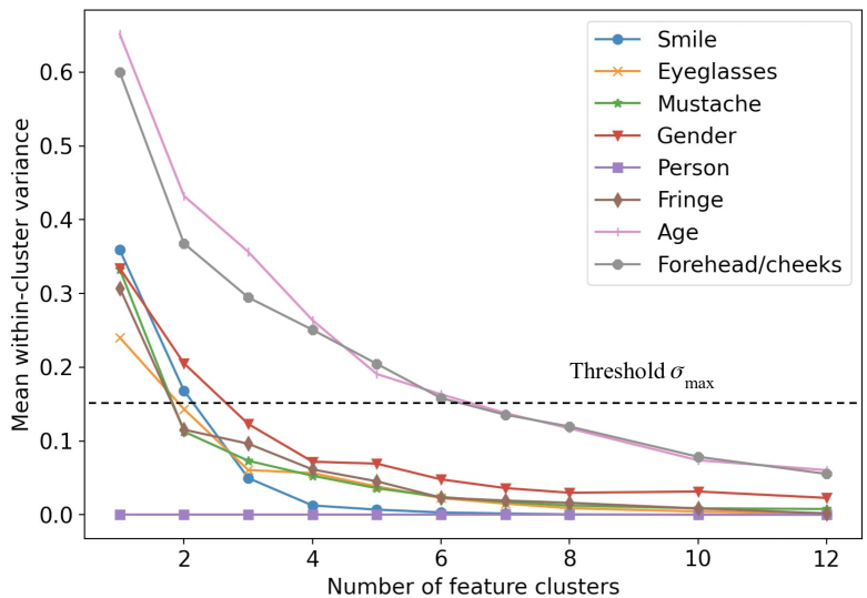
Figure 5: Feature clusters generated from 8 categories of CelebA dataset: setting a lower variance threshold $\sigma_{max}$ will generate more clusters, and a uniform threshold is selected for all categories.

Cluster variance threshold.

Feature clusters are obtained by the second clustering on each concept category so that the mean within-cluster variance is lower than a hyper-parameter $\sigma_{max}$. As in Figure 5, the variance decreases and eventually reaches a plateau as feature cluster number increases. Note that different categories present different variance behavior: for example, the Person category includes the single feature “The person” so variance is always near zero regardless of partitions. Meanwhile, the Age category includes many more feature varieties such as “the thirties”, “the eighties”, “very young”, etc, so it must be divided into more clusters than other categories before the variance drops below the $\sigma_{max}$ threshold. This demonstrates the necessity of using a variance threshold to set the number of feature clusters on a category-by-category basis rather than choosing one fixed cluster number for all categories.

A reasonable $\sigma_{max}$ is required for our algorithm to discover feature correlations: If $\sigma_{max}$ is too small (for example, at or below the plateau region in Figure 5) then redundant clusters are produced for a same feature, which affects the feature’s distribution and thus the correlation measurement. If $\sigma_{max}$ is too large then discrepant features are mixed in a cluster and the cluster’s semantic meaning is lost. The effects of applying CSBD with different values of $\sigma_{max}$ on the CelebA dataset is illustrated in Table 3.

$\sigma_{max}$	0.01	0.05	0.1	0.15	0.2	0.3
$\phi$ coefficient	0.0577	0.0651	0.105	0.106	0.0095	0.0065
Worst ($\uparrow$)	0.897 (1e-3)	0.901 (2e-3)	0.906 (5e-3)	0.908 (3e-3)	NA	NA
Avg. ($\uparrow$)	0.918 (5e-4)	0.919 (3e-3)	0.918 (4e-3)	0.918 (9e-4)	NA	NA

Table 3: Sensitivity analysis on variance threshold $\sigma_{max}$ used for splitting feature clusters. $\sigma_{max}$ of 0.1 and 0.15 generate reasonable feature clusters and accurate correlation ($\phi$ coefficient) between “smile” and “man” features in CelebA, and show better bias mitigation results (Worst). $\sigma_{max}$ of 0.01 and 0.05 generate redundant clusters that impact correlation measurement thus computed intervention. $\sigma_{max}$ bigger than 0.2 generate clusters with ambiguous semantic meanings so no correlation is discovered (NA).

6 Conclusion and Limitation

In this work, we for the first time propose to use textural descriptions for systematic bias discovery and mitigation. The approach leads to a new perspective on bias problems and resolves the limitation of latent space based de-biasing which tends to overlook or mis-identify non-dominant features. Our algorithm applies common-sense reasoning to descriptions generated by humans, which will naturally highlight the features most relevant or noticeable to humans regardless of their size or subtlety in the overall image, and indicates how their correlation to the target will cause downstream bias. Novel sensitive correlations and model biases are discovered for two vision benchmark datasets, and we show state-of-the-art bias mitigation based on the reasoning.

Limitations and future work.

First, our method is limited by the availability of text-based descriptions for an image dataset, though we are not dependant on certain description structures or formats in the text. We do not consider leveraging large pre-trained caption generation models and applying CSBD to the synthetic descriptions in this work, due to the risk of introducing new or additional biases from the caption generation models; however, it may be a worthwhile future research direction. Second, we only study pair-wise feature correlations: higher degrees of correlations and how they affect model performance could be explored. Third, our method has not yet been tested on other vision recognition tasks and models, such as object detection and segmentation. However, since the method for discovering sensitive data feature correlations is agnostic to downstream task, this can be a direct next step.

Supplementary Material

7 Method - mitigation weight setting

In this section, we provide additional details for generating data sampling weights $W(\boldsymbol{t}_{s}|\boldsymbol{t}_{Y})$ used in equation (2). The sampling probabilities are set based on co-occurrence statistics $x_{11},x_{00},x_{10},\text{and }x_{01}$ computed from the feature distributions analyzed by CSBD, described in Sec. 3.

For the sensitive feature $s$, the number of dataset images including $s$ is $x_{1*}$, and the number of dataset images not including $s$ is $x_{0*}$. For the feature’s distribution across the targets: the number of images including $s$ and target feature $y_{i}$ is $x_{11_{i}}$, and the number of images including $y_{i}$ but not $s$ is $x_{01_{i}}$ ($y_{i}\in Y$, where $Y$ is the set of target features).

The intervention is to ensure that images with $s$ have the same distribution across the targets $Y$ as the images without $s$. We denote the sampling probability of images including the $s$ and $y_{i}$ as $p_{sy_{i}}$. It is computed based on the count of feature occurrence $x_{1*}$, $x_{0*}$, and co-occurrence $x_{11_{i}}$, $x_{01_{i}}$ as below:

$$\small p_{sy_{i}}(x_{1*},x_{0*},x_{11_{i}},x_{01_{i}})=\frac{x_{01_{i}}}{x_{0*}}\frac{x_{1*}}{x_{11_{i}}}\text{ for }y_{i}\in Y.$$ (3)

As a result, the feature $s$ distribution with regard to probability:

$$\small P_{D}(\boldsymbol{t}_{s}|\boldsymbol{t}_{Y})W(\boldsymbol{t}_{s}|\boldsymbol{t}_{Y}) =\left[p_{sy_{i}}\frac{x_{11_{i}}}{x_{1*}}\right]\text{ for }y_{i}\in Y$$

$$=\left[\frac{x_{01_{i}}}{x_{0*}}\right]\text{ for }y_{i}\in Y$$

$$=P_{D}(\neg\boldsymbol{t}_{s}|\boldsymbol{t}_{Y}).$$

This is exactly the expression given in equation (2). Thus the re-weighted sampling probabilities will remove the correlation between sensitive feature $s$ and target features.

8 Implementation

8.1 Augmentations

The augmentations used in CSBD, which are implemented alongside the weighted sampling for bias mitigation, are also applied to the other methods for fair comparison. On CelebA we use the following augmentations:

• random resized cropping to 224 $\times$ 224;

• horizontal flips;

• color jitter;

and on MS-COCO we use

• random resized cropping to 448 $\times$ 448;

• horizontal flips;

• RandAugment.

8.2 Training

The following training setups are consistent among comparison methods: We train all classification models for 100 epoches and select the best model on validation set to report its results on testing set. The classification model is ResNet50 [15]. SGD optimizer is used with learning rate of $1e^{-4}$, momentum of 0.9, and weight decay of $0.01$. The batch size is set to be 256 on CelebA dataset and 32 on MS-COCO dataset.

For all other method-specific hyper-parameters, we use the default values in the official repositories for LfF, DebiAN, and BPA, and for PGD we use the default values given in  [1].

9 Results - feature correlation list

We attach the full list of correlated common-sense features discovered by our method, on CelebA dataset (Table 7), and MS-COCO dataset (Table 8 - Table 10). It can be seen that many correlations are benign (that is, that the two features’ co-occurrence is expected), which can only be judged from human knowledge. Therefore, we maintain a human-in-the-loop component to select sensitive/not robust correlations from the lists to treat and mitigate downstream model bias.

10 Results - mitigation results per group

For the downstream bias mitigation experiments on two datasets, Table 1 and Table 2 show the fairness metric (Worst performing group) and the accuracy metric (Group mean accuracy). Here we unpack the results by attaching the performance per group in Table 5 and Table 6, so it can be seen that which sensitive features cause bias result on which targets.

11 Results - embeddings for LfF

The image embedding results for cat classifiers trained with LfF method is shown in Figure 6. Compared to baseline training with no bias mitigation as in Figure 4, the method better mixes the embedding of “No cat” samples across the sensitive features “Couch” and “No couch”. However, the model decision boundary between the two targets “Cat” and “No cat” is not improved: that is, it is still influenced by the existence of the “Couch” feature. As discussed in Sec. 4.4, LfF depends on the model’s decision rule for sensitive feature related samples to de-bias, which fails to distinguish Couch ($\bullet$ $\bullet$) and No couch ($\bullet$ $\bullet$) features in embedding space.

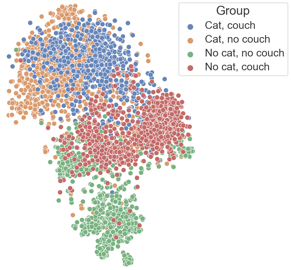
Figure 6: T-SNE results for cat classifiers (“Couch” as sensitive label) trained with MS-COCO dataset. Bias mitigation method LfF [39] is performed.

12 Ablation - category cluster number $C$

In CSBD method, the first clustering on phrase embedding vectors generates $C$ category clusters, and $C$ is a tunable hyper-parameter selected based on the estimation of the dataset’s category diversity. For the CelebA dataset, we use $C=8$. The category clusters are:

1. Age category: “the sixties”, “the forties”, …

2. People title category: “the lady”, “the gentleman, ‘a teenager”, …,

3. Smile category: “a big smile”, “no smile”…,

4. Fringe category: “long bangs”, “medium fringe”…,

5. Eyeglasses category: “thin frame glasses”, “no eyeglasses”…,

6. Beard category: “a very bushy beard”, “no beard”…,

7. Face category: “the whole face”, “the cheeks”…,

8. Other facial attributes: “mouth wide open”, “teeth visible”…

Note that the ordering of the clusters does not matter; we provide an enumerated list here for ease of reference.

We change the value of $C$ to check how this parameter will affect the next steps of generating feature clusters and analyzing feature correlations. Other parameters remain the same as in Sec. 4.2. After performing the second clustering and obtaining the distribution indicators, the $\phi$ correlation coefficients between two feature clusters are computed. We report the $\phi$ coefficient between “Man” and “No smile” features in Table 4. It can be seen that the correlation result is almost invariant to the number of category clusters used. This is expected because though discrepant categories will be mixed in a cluster with a small $C$, the second step which generates feature clusters from a category uses the same variance threshold $\sigma_{max}$, thus will likely generate the same set of feature clusters and their correlations. Thus the hierarchical clustering approach provides some amount of “self-correction” for poorly-chosen values of $C$. However, there is still advantage in identifying a good value of $C$ for a given dataset, namely that the resulting clusters are more intuitive and interpretable when there is no mixing of discrepant categories within a cluster.

$C$	4	5	6	7	8	9	10
$\phi$ coefficient	0.1061	0.1061	0.1057	0.1054	0.106	0.1053	0.1053

Table 4: Sensitivity analysis on category number $C$ used in the first clustering on CelebA dataset. All category numbers can result in accurate feature distribution and correlation measurements.

	Vanilla (no mitigation)	LfF [39]	DebiAN [30]	PGD [1]	BPA [48]	CSBD (ours)
“Smiling”, “Male”	0.894 (3e-3)	0.730 (0.03)	0.895 (0.02)	0.888 (2e-2)	0.899 (3e-3)	0.914 (2e-3)
“Smiling”, Others	0.929 (5e-4)	0.890 (7e-3)	0.905 (2e-2)	0.923 (1e-2)	0.925 (2e-3)	0.935 (1e-3)
“No smile”, “Male”	0.927 (1e-3)	0.911 (2e-2)	0.934 (5e-3)	0.927 (2e-2)	0. 926 (1e-2)	0.908 (5e-3)
“No smile”, Others	0.927 (2e-4)	0.788 (2e-2)	0.930 (1e-2)	0.929 (1e-2)	0.919 (1e-3)	0.915 (3e-3)
“Eyeglasses”, “Male”	0.936 (5e-3)	0.837 (2e-2)	0.917 (2e-2)	0.928 (7e-3)	0.938 (6e-4)	0.939 (1e-3)
“Eyeglasses”, Others	0.926 (4e-3)	0.810 (2e-2)	0.921 (2e-2)	0.917 (1e-2)	0.931 (2e-3)	0.997 (2e-4)
“No eyeglasses”, “Male”	0.991 (1e-4)	0.997 (5e-4)	0.971 (5e-2)	0.997 (4e-4)	0.929 (5e-3)	0.938 (3e-3)
“No eyeglasses”, Others	0.999 (0)	0.999 (0)	0.973 (5e-2)	0.999 (0)	0.999 (0)	0.999 (0)

Table 5: The downstream classification results per group (combinations of target label and sensitive feature label pairs) on CelebA dataset. The mean accuracy and standard deviation is reported based on three independent runs.

Group	Vanilla (no mitigation)	LfF [39]	DebiAN [30]	PGD [1]	BPA [48]	CSBD (ours)
“Cat”, “Couch”	0.942 (8e-3)	0.942 (7e-3)	0.913 (8e-3)	0.935 (8e-3)	0.918 (2e-2)	0.917 (6e-3)
“Cat”, “No couch”	0.955 (5e-3)	0.944 (5e-3)	0.938 (1e-2)	0.949 (6e-3)	0.950 (2e-2)	0.948 (6e-3)
“No cat”, “Couch”	0.849 (5e-2)	0.8 (5e-2)	0.793 (5e-2)	0.884 (1e-2)	0.853 (4e-2)	0.908 (7e-3)
“No cat”, “No couch”	0.992 (2e-3)	0.976 (4e-4)	0.964 (1e-2)	0.993 (7e-4)	0.979 (6e-3)	0.989 (3e-3)
“Cat”, “Keyboard”	0.974 (0)	0.974 (0)	0.978 (2e-2)	0.974 (0)	0.982 (8e-3)	0.974 (0)
“Cat”, “No keyboard”	0.949 (1e-3)	0.942 (5e-3)	0.930 (1e-2)	0.948 (8e-4)	0.941 (1e-3)	0.954 (8e-4)
“No cat”, “Keyboard”	0.986 (3e-2)	0.870 (4e-2)	0.855 (0.14)	1 (0)	0.913 (9e-2)	1 (0)
“No cat”, “No keyboard”	0.978 (5e-3)	0.966 (4e-3)	0.954 (1e-2)	0.984 (2e-3)	0.971 (7e-3)	0.977 (3e-3)
“Dog”, “Frisbee”	0.963 (5e-3)	0.979 (5e-3)	0.927 (7e-3)	0.965 (8e-3)	0.955 (2e-2)	0.965 (6e-3)
“Dog”, “No frisbee”	0.890 (4e-4)	0.892 (2e-2)	0.845 (2e-2)	0.872 (7e-3)	0.881 (1e-2)	0.906 (9e-3)
“No dog”, “Frisbee”	0.903 (3e-2)	0.828 (7e-2)	0.903 (0)	0.957 (2e-2)	0.860 (4e-2)	0.946 (2e-2)
“No dog”, “No frisbee”	0.952 (3e-3)	0.874 (8e-3)	0.906 (2e-2)	0.967 (8e-3)	0.924 (2e-2)	0.920 (1e-2)
“TV”, “Chair”	0.960 (4e-3)	0.948 (4e-3)	0.959 (3e-3)	0.944 (3e-3)	0.945 (3e-3)	0.941 (2e-3)
“TV”, “No chair”	0.924 (5e-3)	0.891 (9e-3)	0.904 (2e-2)	0.889 (2e-2)	0.897 (1e-2)	0.907 (2e-3)
“No TV”, “Chair”	0.726 (1e-2)	0.690 (2e-2)	0.718 (2e-2)	0.821 (9e-3)	0.758 (2e-2)	0.842 (9e-3)
“No TV”, “No chair”	0.96 (5e-3)	0.939 (9e-3)	0.923 (1e-2)	0.972 (4e-3)	0.949 (7e-3)	0.956 (1e-3)
“Umbrella”, “People”	0.906 (6e-3)	0.897 (1e-2)	0.876 (2e-2)	0.886 (5e-3)	0.897 (9e-3)	0.891 (1e-2)
“Umbrella”, “No people”	0.761 (1e-2)	0.771 (5e-3)	0.716 (5e-2)	0.763 (2e-2)	0.777 (2e-2)	0.814 (1e-2)
“No umbrella”, “People”	0.880 (6e-3)	0.803 (3e-2)	0.870 (2e-2)	0.918 (7e-3)	0.877 (1e-2)	0.904 (9e-3)
“No umbrella”, “No people”	0.974 (5e-3)	0.947 (7e-3)	0.966 (5e-3)	0.979 (3e-3)	0.959 (6e-3)	0.961 (3e-3)
“Kite”, “People”	0.969 (5e-3)	0.953 (5e-3)	0.959 (5e-3)	0.946 (4e-3)	0.981 (6e-3)	0.959 (4e-3)
“Kite”, “No people”	0.961 (4e-3)	0.854 (2e-2)	0.951 (3e-2)	0.917 (0)	0.924 (1e-2)	0.951 (1e-2)
“No kite”, “People”	0.938 (0)	0.919 (3e-2)	0.954 (5e-3)	0.972 (0)	0.939 (1e-2)	0.957 (1e-2)
“No kite”, “No people”	0.985 (0)	0.966 (1e-2)	0.975 (3e-3)	0.988 (3e-3)	0.983 (2e-3)	0.973 (9e-3)

Table 6: The downstream classification results per group (combinations of target label and sensitive feature label pairs) on MS-COCO dataset. The mean accuracy and standard deviation is reported based on three independent runs.

Feature 1	Feature 2	$\phi$ correlation coefficient
“thick/thin frame”	“eyeglasses”	0.1243
“thick/thin frame”	“no eyeglasses”	-0.1328
“eyeglasses”	“man”	0.0693
“eyeglasses”	“woman”	-0.0743
“no eyeglasses”	“man”	-0.0681
“no eyeglasses”	“woman”	0.0734
“forehead”	“eyeglasses”	0.0609
“forehead”	“a small portion”	0.3503
“the face”	“no eyeglasses”	-0.1849
“the face”	“eyeglasses”	0.1862
“the face”	“no smile”	0.0802
“the face”	“a smile”	-0.1012
“the face”	“happiness”	0.1261
“teeth visible”	“no smile”	-0.3348
“teeth visible”	“a smile”	0.2571
“mouth wide open”	“no smile”	-0.1826
“mouth wide open”	“happiness”	-0.0934
“mouth wide open”	“teeth visible”	0.1202
“a little bit open”	“the face”	-0.068
“forehead”	“man”	-0.0637
“forehead”	“woman”	0.0649
“no smile”	“happiness”	-0.2961
“no smile”	“teenager”	0.0506
“no smile”	“man”	0.1058
“a smile”	“man”	-0.0552
“man”	“the middle age”	0.0817
“man”	“medium length”	0.2204
“man”	“forties”, “fifties”	0.0627
“beard”	“the middle age”	0.056
“mustache”	“the middle age”	0.0601
“beard”	“ middle length”	0.18
“mustache”	“ middle length”	0.1921
“beard”	“teenager”	-0.0504
“mustache”	“ teenager”	-0.0527
“beard”	“no smile”	0.0754
“mustache”	“ no smile”	0.0788
“beard”	“woman”	-0.3988
“mustache”	“woman”	-0.3939
“beard”	“man”	0.4498
“mustache”	“man”	0.4482

Table 7: The correlated feature pairs in CelebA dataset, reasoned by CSBD. Each feature is a cluster of descriptive phrases and only 1-2 representative phrases are shown in the table.

Feature 1	Feature 2	$\phi$ correlation coefficient
“soccer”, “baseball”	“field”	0.1246
“baseball bat”	“field”	0.0902
“soccer”, “baseball”	“the ball”	0.1638
“soccer”, “baseball”	“a game”	0.149
“baseball bat”	“a ball”	0.1089
“soccer”, “baseball”	“a man”, “a boy”	0.0673
“sky”, “ air”	“a man”, “a boy”	0.0558
“sky”, “ air”	“skateboard”	0.1252
“sky”, “ air”	“snowboard”	0.0903
“sky”, “ air”	“airplane”	0.0901
“sky”, “ air”	“kite”	0.1024
“men”	“a group”	0.085
“a man”	“a group”	-0.0666
“a man”	“frisbee”	0.0701
“a man”	“skateboard”	0.1263
“a man”	“snowboard”	0.0885
“men”	“two members”	0.0768
“men”	“two members”	0.0768
“a man”	“cellphone”	0.0523
“a man”	“hand”, “fingers”	0.051
“a man”	“tennis racket”	0.0674
“a man”	“tennis player”	0.0758
“a man”	“umbrella”	0.062
“men”	“sneakers”, “pants”	0.0621
“a man”	“wave”	0.0969
“a man”	“surfboard”	0.1102
“zebra”	“ grass field”	0.1454
“giraffe”	“ grass field”	0.1022
“zebra”	“sheep”	0.077
“zebra”	“trees”	0.0834
“giraffe”	“trees”	0.1644
“giraffe”	“fence”	0.0745
“a person”	“snowy slopes”	0.084
“a person”	“ skateboard”	0.0635
“a person”	“snowboard”	0.0748
“bike”	“city street”	0.0675
“motorcycle”	“city street”	0.0504
“motorcycle”	“road”	0.0677
“bus”	“city street”	0.1364
“bus”	“road”	0.1072
“bathroom”	“ vase”	0.1229
“sink”	“window”	0.085
“bathroom”	“window”	0.1092
“sink”	“toilet”	0.1667
“bathroom”	“toilet”	0.423
“snowy slopes”	“snowboard”	0.1701
“table”	“food”	0.1723
“table”	“pizza”	0.1123
“table”	“cake”	0.081
“table”	“beverages”	0.1173
“table”	“flower”	0.0642
“table”	“plate”	0.123
“table”	“bowl”, ‘cup”	0697
“table”	“fresh produce”	0.0634
“table”	“vase”	0.079
“table”	“glasses”	0.0578
“food”	“kitchen”	0.0703
“food”	“plate”	0.2588
“food”	“a dish”	0.0693
“food”	“bowl”, ‘cup”	0.0516
“food”	“egg”, “sausage”	0.0545
“living room”	“game controller”	0.0574
“living room”	“pillow”	0.1643
“couch”	“dog”	0.058
“couch”	“cat”	0.0615

Table 8: The correlated feature pairs in MS-COCO dataset, reasoned by CSBD. Each feature is a cluster of descriptive phrases and only 1-2 representative phrases are shown in the table.

Feature 1	Feature 2	$\phi$ correlation coefficient
“the top”, “the front”	“clock”	0.0594
“the top”, “the front”	“car”	0.0543
“microwave”, “oven”	“dishes”	0.0604
“kitchen”	“scissors”	0.0894
“a group”	“a game”	0.0588
“a group”	“people”	0.3927
“frisbee”	“field”	0.0616
“frisbee”	“a game”	0.0994
“frisbee”	“dog”	0.091
“plate”	“pizza”	0.1148
“plate”	“cake”	0.1013
“plate”	“sandwich”	0.2136
“plate”	“donuts”	0.0614
“plate”	“meat”	0.1573
“plate”	“vegetables”	0.1855
“plate”	“snacks”	0.1307
“plate”	“hot dogs”	0.0594
“plate”	“fruits”	0.074
“plate”	“beverages”	0.0627
“bowl”, “cup”	“sandwich”	0.069
“bowl”, “cup”	“beverages”	0.1497
“bowl”, “cup”	“fruit”	0.1396
“bowl”, “cup”	“vegetables”	0.1079
“bowl”, “cup”	“bananas”	0.0625
“glasses”	“beverages”	0.136
“a pot”	“beverages”	0.0942
“a pot”	“flower”	0.2277
“sandwich”	“beverages”	0.0537
“sandwich”	“meat”	0.0725
“sandwich”	“vegetables”	0.0812
“hot dogs”	“vegetables”	0.1717
“donuts”	“beverages”	0.0515
“pizza”	“vegetables”	0.1046
“pizza”	“box”	0.0784
“cake”	“box”	0.1151
“donuts”	“box”	0.0664
“tray”	“pizza”	0.1309
“tray”	“cake”	0.0529
“tray”	“sandwich”	0.0586
“tray”	“vegetables”	0.105
“dish”	“vegetables”	0.0836
“skateboard”	“a line drive”	0.0849
“skateboard”	“boys”	0.1404
“grass field”	“cow”	0.1226
“grass field”	“sheep”	0.184
“grass field”	“elephant”	0.0516
“field”	“trees”	0.063
“sheep”	“birds”	0.0794
“bed”	“chairs”	0.051
“bedroom”	“chairs”	0.057
“bedroom”	“furniture”	0.0852
“bed”	“cat”	0.0609
“bags”	“a pack”	0.0506
“city”	“traffic lights”	0.0682
“cell phone”	“women”	0.0721
“desk”	“cat”	0.0753
“keyboard”	“cat”	0.1
“beach”	“kite”	0.1347
“beach”	“people”	0.0789
“beach”	“surfer”	0.1594
“beach”	“umbrella”	0.0768
“water”, “ocean”	“boat”	0.1235
“water”, “ocean”	“birds”	0.0558
“water”, “ocean”	“shore”	0.1412
“water”, “ocean”	“surfer”	0.2677

Table 9: The correlated feature pairs in MS-COCO dataset, reasoned by CSBD. Each feature is a cluster of descriptive phrases and only 1-2 representative phrases are shown in the table.

Feature 1	Feature 2	$\phi$ correlation coefficient
“a woman”	“tennis player”	0.0902
“a woman”	“umbrella”	0.0688
“city street”	“sign”	0.0743
“city street”	“traffic light”	0.1255
“fruit”	“a bunch”	0.0644
“bananas”	“a bunch”	0.0938
“clock”	“building”	0.1026
“airplane”	“airport”	0.1426
“trees”	“elephant”	0.0637
“a ball”	“tennis player”	0.1709
“a ball”	“tennis racket”	0.0833
“a ball”	“tennis court”	0.0827
“tennis court”	“a game”	0.0595
“a game”	“controllers”	0.1199
“a game”	“a man”	0.0642
“window”	“cat ”	0.0574
“building”	“sign”	0.056
“a flattened area”	“train”	0.093
“boat”	“water flow”	0.0802
“fence”	“sign”	0.1064
“umbrella”	“people”	0.1001
“kite”	“people”	0.1023
“birds”	“water flow”	0.0522
“people”	“a crowd”	0.097

Table 10: The correlated feature pairs in MS-COCO dataset, reasoned by CSBD. Each feature is a cluster of descriptive phrases and only 1-2 representative phrases are shown in the table.

References

- Ahn et al. [2022] Sumyeong Ahn, Seongyoon Kim, and Se-young Yun. Mitigating dataset bias by using per-sample gradient. arXiv preprint arXiv:2205.15704, 2022.
- Alayrac et al. [2022] Jean-Baptiste Alayrac, Jeff Donahue, Pauline Luc, Antoine Miech, Iain Barr, Yana Hasson, Karel Lenc, Arthur Mensch, Katherine Millican, Malcolm Reynolds, et al. Flamingo: a visual language model for few-shot learning. Advances in Neural Information Processing Systems, 35:23716–23736, 2022.
- Amini et al. [2018] Alexander Amini, Wilko Schwarting, Guy Rosman, Brandon Araki, Sertac Karaman, and Daniela Rus. Variational autoencoder for end-to-end control of autonomous driving with novelty detection and training de-biasing. In 2018 IEEE/RSJ International Conference on Intelligent Robots and Systems (IROS), pages 568–575. IEEE, 2018.
- Amini et al. [2019] Alexander Amini, Ava P Soleimany, Wilko Schwarting, Sangeeta N Bhatia, and Daniela Rus. Uncovering and mitigating algorithmic bias through learned latent structure. In Proceedings of the 2019 AAAI/ACM Conference on AI, Ethics, and Society, pages 289–295, 2019.
- Antol et al. [2015] Stanislaw Antol, Aishwarya Agrawal, Jiasen Lu, Margaret Mitchell, Dhruv Batra, C Lawrence Zitnick, and Devi Parikh. Vqa: Visual question answering. In Proceedings of the IEEE international conference on computer vision, pages 2425–2433, 2015.
- Bahng et al. [2020] Hyojin Bahng, Sanghyuk Chun, Sangdoo Yun, Jaegul Choo, and Seong Joon Oh. Learning de-biased representations with biased representations. In International Conference on Machine Learning, pages 528–539. PMLR, 2020.
- Basu et al. [2023] Abhipsa Basu, R Venkatesh Babu, and Danish Pruthi. Inspecting the geographical representativeness of images from text-to-image models. arXiv preprint arXiv:2305.11080, 2023.
- Bommasani et al. [2021] Rishi Bommasani, Drew A Hudson, Ehsan Adeli, Russ Altman, Simran Arora, Sydney von Arx, Michael S Bernstein, Jeannette Bohg, Antoine Bosselut, Emma Brunskill, et al. On the opportunities and risks of foundation models. arXiv preprint arXiv:2108.07258, 2021.
- Brown et al. [2023] Alexander Brown, Nenad Tomasev, Jan Freyberg, Yuan Liu, Alan Karthikesalingam, and Jessica Schrouff. Detecting shortcut learning for fair medical ai using shortcut testing. Nature Communications, 14(1):4314, 2023.
- Cer et al. [2018] Daniel Cer, Yinfei Yang, Sheng-yi Kong, Nan Hua, Nicole Limtiaco, Rhomni St John, Noah Constant, Mario Guajardo-Cespedes, Steve Yuan, Chris Tar, et al. Universal sentence encoder. arXiv preprint arXiv:1803.11175, 2018.
- Chen et al. [2015] Xinlei Chen, Hao Fang, Tsung-Yi Lin, Ramakrishna Vedantam, Saurabh Gupta, Piotr Dollár, and C Lawrence Zitnick. Microsoft coco captions: Data collection and evaluation server. arXiv preprint arXiv:1504.00325, 2015.
- Cramér [1946] Harald Cramér. Mathematical methods of statistics. 1946.
- Diomataris et al. [2021] Markos Diomataris, Nikolaos Gkanatsios, Vassilis Pitsikalis, and Petros Maragos. Grounding consistency: Distilling spatial common sense for precise visual relationship detection. In Proceedings of the IEEE/CVF International Conference on Computer Vision, pages 15911–15920, 2021.
- Dunlap et al. [2022] Lisa Dunlap, Clara Mohri, Devin Guillory, Han Zhang, Trevor Darrell, Joseph E Gonzalez, Aditi Raghunathan, and Anna Rohrbach. Using language to extend to unseen domains. In The Eleventh International Conference on Learning Representations, 2022.
- He et al. [2016] Kaiming He, Xiangyu Zhang, Shaoqing Ren, and Jian Sun. Deep residual learning for image recognition. In Proceedings of the IEEE conference on computer vision and pattern recognition, pages 770–778, 2016.
- Hendrycks and Dietterich [2019] Dan Hendrycks and Thomas Dietterich. Benchmarking neural network robustness to common corruptions and perturbations. arXiv preprint arXiv:1903.12261, 2019.
- Jia et al. [2021] Chao Jia, Yinfei Yang, Ye Xia, Yi-Ting Chen, Zarana Parekh, Hieu Pham, Quoc Le, Yun-Hsuan Sung, Zhen Li, and Tom Duerig. Scaling up visual and vision-language representation learning with noisy text supervision. In International conference on machine learning, pages 4904–4916. PMLR, 2021.
- Jiang et al. [2021] Yuming Jiang, Ziqi Huang, Xingang Pan, Chen Change Loy, and Ziwei Liu. Talk-to-edit: Fine-grained facial editing via dialog. In Proceedings of the IEEE/CVF International Conference on Computer Vision, pages 13799–13808, 2021.
- Jolliffe [2002] Ian T Jolliffe. Principal component analysis for special types of data. Springer, 2002.
- Karpathy and Fei-Fei [2015] Andrej Karpathy and Li Fei-Fei. Deep visual-semantic alignments for generating image descriptions. In Proceedings of the IEEE conference on computer vision and pattern recognition, pages 3128–3137, 2015.
- Khattak et al. [2023] Muhammad Uzair Khattak, Hanoona Rasheed, Muhammad Maaz, Salman Khan, and Fahad Shahbaz Khan. Maple: Multi-modal prompt learning. In Proceedings of the IEEE/CVF Conference on Computer Vision and Pattern Recognition, pages 19113–19122, 2023.
- Kim et al. [2021] Eungyeup Kim, Jihyeon Lee, and Jaegul Choo. Biaswap: Removing dataset bias with bias-tailored swapping augmentation. In Proceedings of the IEEE/CVF International Conference on Computer Vision, pages 14992–15001, 2021.
- Krishnakumar et al. [2021] Arvindkumar Krishnakumar, Viraj Prabhu, Sruthi Sudhakar, and Judy Hoffman. Udis: Unsupervised discovery of bias in deep visual recognition models. In British Machine Vision Conference (BMVC), page 3, 2021.
- Lake et al. [2017] Brenden M Lake, Tomer D Ullman, Joshua B Tenenbaum, and Samuel J Gershman. Building machines that learn and think like people. Behavioral and brain sciences, 40:e253, 2017.
- Lang et al. [2021] Oran Lang, Yossi Gandelsman, Michal Yarom, Yoav Wald, Gal Elidan, Avinatan Hassidim, William T Freeman, Phillip Isola, Amir Globerson, Michal Irani, et al. Explaining in style: Training a gan to explain a classifier in stylespace. In Proceedings of the IEEE/CVF International Conference on Computer Vision, pages 693–702, 2021.
- LeCun and Cortes [2010] Yann LeCun and Corinna Cortes. MNIST handwritten digit database. 2010.
- Li and Deng [2020] Shan Li and Weihong Deng. A deeper look at facial expression dataset bias. IEEE Transactions on Affective Computing, 13(2):881–893, 2020.
- Li and Vasconcelos [2019] Yi Li and Nuno Vasconcelos. Repair: Removing representation bias by dataset resampling. In Proceedings of the IEEE/CVF conference on computer vision and pattern recognition, pages 9572–9581, 2019.
- Li and Xu [2021] Zhiheng Li and Chenliang Xu. Discover the unknown biased attribute of an image classifier. In Proceedings of the IEEE/CVF International Conference on Computer Vision, pages 14970–14979, 2021.
- Li et al. [2022] Zhiheng Li, Anthony Hoogs, and Chenliang Xu. Discover and mitigate unknown biases with debiasing alternate networks. In European Conference on Computer Vision, pages 270–288. Springer, 2022.
- Lin et al. [2014] Tsung-Yi Lin, Michael Maire, Serge Belongie, James Hays, Pietro Perona, Deva Ramanan, Piotr Dollár, and C Lawrence Zitnick. Microsoft coco: Common objects in context. In Computer Vision–ECCV 2014: 13th European Conference, Zurich, Switzerland, September 6-12, 2014, Proceedings, Part V 13, pages 740–755. Springer, 2014.
- Liu et al. [2021] Evan Z Liu, Behzad Haghgoo, Annie S Chen, Aditi Raghunathan, Pang Wei Koh, Shiori Sagawa, Percy Liang, and Chelsea Finn. Just train twice: Improving group robustness without training group information. In International Conference on Machine Learning, pages 6781–6792. PMLR, 2021.
- Liu et al. [2015] Ziwei Liu, Ping Luo, Xiaogang Wang, and Xiaoou Tang. Deep learning face attributes in the wild. In Proceedings of the IEEE international conference on computer vision, pages 3730–3738, 2015.
- Lloyd [1982] Stuart Lloyd. Least squares quantization in pcm. IEEE transactions on information theory, 28(2):129–137, 1982.
- Manjunatha et al. [2019] Varun Manjunatha, Nirat Saini, and Larry S Davis. Explicit bias discovery in visual question answering models. In Proceedings of the IEEE/CVF Conference on Computer Vision and Pattern Recognition, pages 9562–9571, 2019.
- Matthews [1975] Brian W. Matthews. Comparison of the predicted and observed secondary structure of t4 phage lysozyme. Biochimica et biophysica acta, 405 2:442–51, 1975.
- McInnes et al. [2018] Leland McInnes, John Healy, and James Melville. Umap: Uniform manifold approximation and projection for dimension reduction. arXiv preprint arXiv:1802.03426, 2018.
- Misra et al. [2016] Ishan Misra, C Lawrence Zitnick, Margaret Mitchell, and Ross Girshick. Seeing through the human reporting bias: Visual classifiers from noisy human-centric labels. In Proceedings of the IEEE conference on computer vision and pattern recognition, pages 2930–2939, 2016.
- Nam et al. [2020] Junhyun Nam, Hyuntak Cha, Sungsoo Ahn, Jaeho Lee, and Jinwoo Shin. Learning from failure: De-biasing classifier from biased classifier. Advances in Neural Information Processing Systems, 33:20673–20684, 2020.
- Park et al. [2022] Sungho Park, Jewook Lee, Pilhyeon Lee, Sunhee Hwang, Dohyung Kim, and Hyeran Byun. Fair contrastive learning for facial attribute classification. In Proceedings of the IEEE/CVF Conference on Computer Vision and Pattern Recognition, pages 10389–10398, 2022.
- Pearson [1900] Karl Pearson. X. on the criterion that a given system of deviations from the probable in the case of a correlated system of variables is such that it can be reasonably supposed to have arisen from random sampling. The London, Edinburgh, and Dublin Philosophical Magazine and Journal of Science, 50(302):157–175, 1900.
- Qraitem et al. [2023] Maan Qraitem, Kate Saenko, and Bryan A Plummer. Bias mimicking: A simple sampling approach for bias mitigation. In Proceedings of the IEEE/CVF Conference on Computer Vision and Pattern Recognition, pages 20311–20320, 2023.
- Radford et al. [2019] Alec Radford, Jeffrey Wu, Rewon Child, David Luan, Dario Amodei, Ilya Sutskever, et al. Language models are unsupervised multitask learners. OpenAI blog, 1(8):9, 2019.
- Radford et al. [2021] Alec Radford, Jong Wook Kim, Chris Hallacy, Aditya Ramesh, Gabriel Goh, Sandhini Agarwal, Girish Sastry, Amanda Askell, Pamela Mishkin, Jack Clark, et al. Learning transferable visual models from natural language supervision. In International conference on machine learning, pages 8748–8763. PMLR, 2021.
- Ramaswamy et al. [2021] Vikram V Ramaswamy, Sunnie SY Kim, and Olga Russakovsky. Fair attribute classification through latent space de-biasing. In Proceedings of the IEEE/CVF conference on computer vision and pattern recognition, pages 9301–9310, 2021.
- Rombach et al. [2022] Robin Rombach, Andreas Blattmann, Dominik Lorenz, Patrick Esser, and Björn Ommer. High-resolution image synthesis with latent diffusion models. In Proceedings of the IEEE/CVF conference on computer vision and pattern recognition, pages 10684–10695, 2022.
- Schramowski et al. [2022] Patrick Schramowski, Cigdem Turan, Nico Andersen, Constantin A Rothkopf, and Kristian Kersting. Large pre-trained language models contain human-like biases of what is right and wrong to do. Nature Machine Intelligence, 4(3):258–268, 2022.
- Seo et al. [2022] Seonguk Seo, Joon-Young Lee, and Bohyung Han. Unsupervised learning of debiased representations with pseudo-attributes. In Proceedings of the IEEE/CVF Conference on Computer Vision and Pattern Recognition, pages 16742–16751, 2022.
- Sharma et al. [2020] Shubham Sharma, Yunfeng Zhang, Jesús M Ríos Aliaga, Djallel Bouneffouf, Vinod Muthusamy, and Kush R Varshney. Data augmentation for discrimination prevention and bias disambiguation. In Proceedings of the AAAI/ACM Conference on AI, Ethics, and Society, pages 358–364, 2020.
- Singh et al. [2020] Krishna Kumar Singh, Dhruv Mahajan, Kristen Grauman, Yong Jae Lee, Matt Feiszli, and Deepti Ghadiyaram. Don’t judge an object by its context: Learning to overcome contextual bias. In Proceedings of the IEEE/CVF Conference on Computer Vision and Pattern Recognition, pages 11070–11078, 2020.
- Sohn et al. [2023] Kihyuk Sohn, Huiwen Chang, José Lezama, Luisa Polania, Han Zhang, Yuan Hao, Irfan Essa, and Lu Jiang. Visual prompt tuning for generative transfer learning. In Proceedings of the IEEE/CVF Conference on Computer Vision and Pattern Recognition, pages 19840–19851, 2023.
- Sohoni et al. [2020] Nimit Sohoni, Jared Dunnmon, Geoffrey Angus, Albert Gu, and Christopher Ré. No subclass left behind: Fine-grained robustness in coarse-grained classification problems. Advances in Neural Information Processing Systems, 33:19339–19352, 2020.
- Tian et al. [2022] Huan Tian, Tianqing Zhu, Wei Liu, and Wanlei Zhou. Image fairness in deep learning: problems, models, and challenges. Neural Computing and Applications, 34(15):12875–12893, 2022.
- Torralba and Efros [2011] Antonio Torralba and Alexei A Efros. Unbiased look at dataset bias. In CVPR 2011, pages 1521–1528. IEEE, 2011.
- Truong et al. [2023] Thanh-Dat Truong, Ngan Le, Bhiksha Raj, Jackson Cothren, and Khoa Luu. Fredom: Fairness domain adaptation approach to semantic scene understanding. In Proceedings of the IEEE/CVF Conference on Computer Vision and Pattern Recognition, pages 19988–19997, 2023.
- Wang and Russakovsky [2023] Angelina Wang and Olga Russakovsky. Overwriting pretrained bias with finetuning data. In Proceedings of the IEEE/CVF International Conference on Computer Vision, pages 3957–3968, 2023.
- Wang et al. [2019] Danding Wang, Qian Yang, Ashraf Abdul, and Brian Y Lim. Designing theory-driven user-centric explainable ai. In Proceedings of the 2019 CHI conference on human factors in computing systems, pages 1–15, 2019.
- Wang et al. [2020] Zeyu Wang, Klint Qinami, Ioannis Christos Karakozis, Kyle Genova, Prem Nair, Kenji Hata, and Olga Russakovsky. Towards fairness in visual recognition: Effective strategies for bias mitigation. In Proceedings of the IEEE/CVF conference on computer vision and pattern recognition, pages 8919–8928, 2020.
- Wu et al. [2019] Hao Wu, Jiayuan Mao, Yufeng Zhang, Yuning Jiang, Lei Li, Weiwei Sun, and Wei-Ying Ma. Unified visual-semantic embeddings: Bridging vision and language with structured meaning representations. In Proceedings of the IEEE/CVF Conference on Computer Vision and Pattern Recognition, pages 6609–6618, 2019.
- Wu et al. [2023] Shirley Wu, Mert Yuksekgonul, Linjun Zhang, and James Zou. Discover and cure: Concept-aware mitigation of spurious correlation. arXiv preprint arXiv:2305.00650, 2023.
- Wu et al. [2022] Xingjiao Wu, Luwei Xiao, Yixuan Sun, Junhang Zhang, Tianlong Ma, and Liang He. A survey of human-in-the-loop for machine learning. Future Generation Computer Systems, 135:364–381, 2022.
- Yuan et al. [2021] Lu Yuan, Dongdong Chen, Yi-Ling Chen, Noel Codella, Xiyang Dai, Jianfeng Gao, Houdong Hu, Xuedong Huang, Boxin Li, Chunyuan Li, et al. Florence: A new foundation model for computer vision. arXiv preprint arXiv:2111.11432, 2021.
- Zhang et al. [2022a] Fengda Zhang, Kun Kuang, Long Chen, Yuxuan Liu, Chao Wu, and Jun Xiao. Fairness-aware contrastive learning with partially annotated sensitive attributes. In The Eleventh International Conference on Learning Representations, 2022a.
- Zhang et al. [2022b] Haotian Zhang, Pengchuan Zhang, Xiaowei Hu, Yen-Chun Chen, Liunian Li, Xiyang Dai, Lijuan Wang, Lu Yuan, Jenq-Neng Hwang, and Jianfeng Gao. Glipv2: Unifying localization and vision-language understanding. Advances in Neural Information Processing Systems, 35:36067–36080, 2022b.
- Zhang et al. [2022c] Michael Zhang, Nimit S Sohoni, Hongyang R Zhang, Chelsea Finn, and Christopher Ré. Correct-n-contrast: A contrastive approach for improving robustness to spurious correlations. arXiv preprint arXiv:2203.01517, 2022c.
- Zhang et al. [2023a] Xu Zhang, Wen Wang, Zhe Chen, Yufei Xu, Jing Zhang, and Dacheng Tao. Clamp: Prompt-based contrastive learning for connecting language and animal pose. In Proceedings of the IEEE/CVF Conference on Computer Vision and Pattern Recognition, pages 23272–23281, 2023a.
- Zhang et al. [2023b] Yuhui Zhang, Jeff Z HaoChen, Shih-Cheng Huang, Kuan-Chieh Wang, James Zou, and Serena Yeung. Diagnosing and rectifying vision models using language. arXiv preprint arXiv:2302.04269, 2023b.
- Zhong et al. [2022] Yiwu Zhong, Jianwei Yang, Pengchuan Zhang, Chunyuan Li, Noel Codella, Liunian Harold Li, Luowei Zhou, Xiyang Dai, Lu Yuan, Yin Li, et al. Regionclip: Region-based language-image pretraining. In Proceedings of the IEEE/CVF Conference on Computer Vision and Pattern Recognition, pages 16793–16803, 2022.