Assessing Inf luential Observations in Pain Prediction using fMRI Data

Abstract

Neuroimaging has provided invaluable insight into our understanding of human behavior. Modern analytic approaches combine methodological advances in data acquisition with predictive modeling to map patterns of brain activity onto mental states and behaviors. However, in modeling multivariate patterns of brain activity, the existence of subjects with unusual characteristics could potentially undermine the generalizability of the findings. Attempts to detect and account for these subjects have to date has been sorely lacking in the neuroimgaing domain. In addition, most existing methods for performing inf luential diagnosis, presume a deterministic submodel and are designed for low-dimensional data (i.e., the number of predictors $p$ is smaller than the sample size $n$). However, the stochastic selection of a submodel from high-dimensional data where $p$ exceeds $n$ has become ubiquitous in a wide range of scientific areas including neuroimaging. Therefore, methods for identifying observations that could exert undue inf luence on the choice of a submodel promises to play an important role. To date, discussion of this topic has been limited, falling short in two ways: (i) constrained ability to detect multiple inf luential points, and (ii) applicability only in restrictive settings. After describing the problem, we characterize and formalize the concept of inf luential observations on variable selection. Then, we propose a generalized diagnostic measure, extended from an available metric accommodating different model selectors and multiple inf luential observations, the asymptotic distribution of which is subsequently established for large $p$, thus providing guidelines to ascertain inf luential observations. A high-dimensional clustering procedure is further incorporated into our proposed scheme to detect multiple inf luential points. Simulation is conducted to assess the performances of various diagnostic approaches. The proposed procedure is shown to improve predictive power when analyzing thermal-stimulated pain based on fMRI data.

, and

1 Introduction

Neuroimaging is poised to take a substantial leap forward in uncovering the neurophysiological underpinnings of human behavior. This is primarily being driven by the improved analytic and computational capabilities provided by artificial intelligence, machine learning, and associated statistical techniques. This promises the creation of complex brain models, using multivariate patterns of brain activity as input, that will allow us to better understand the functional representations underlying behavior, performance, clinical status and prognosis (Orru et al., 2012; Haynes, 2015). To reach their full potential, it is critical that these models be robust and generalizable across individuals, with strong performance on new, out-of-sample participants. However, the existence of subjects with unusual traits or data could unduly influence the data-dependent formation of the resulting brain models. Therefore, when developing such approaches, it is critical to identify when this occurs to ensure the generalizability of the proposed statistical models.

During the course of a task-based functional magnetic resonance imaging (fMRI) study, a number of subjects receive one or more stimuli while their brain activation is measured at hundreds of time points. The measurement at each time point consists of the subject’s blood oxygenation level dependent (BOLD) response at a large number of spatial locations (voxels), thus giving rise to multivariate time series data. To perform proper statistical analysis at the population-level, it is necessary for voxels to lie in the same location across subjects. The preprocessing of fMRI data therefore includes using nonlinear transformations to transform individual subjects’ anatomical data to a common reference space (e.g., “Montreal Neurologic Institute” (MNI) space). The transformations are thereafter applied to the functional data, allowing for the direct comparison of data across subjects (Lindquist et al., 2008; Ombao et al., 2016). Next, for each subject, a voxel-wise general linear model (GLM) analysis is performed and the estimated regression coefficient corresponding to the task-specific regressor at each voxel is combined into a single subject-specific 3D activation map. This data is used as features in a predictive model. For the model to be generalizable it is important that the data is both comparable across subjects and measuring equivalent phenomena.

As a motivating example, consider the prediction of physical pain using brain activation measures obtained from fMRI data (Lindquist et al., 2017). Pain is associated with large social and economic costs. However, it is primarily assessed via self-report, making it hard to accurately determine. Recently, predictive models have been used to derive patterns of activity across brain regions that provide direct measures of pain intensity (Wager et al., 2013a; Lindquist et al., 2017). However, to be clinically useful these models must exhibit high sensitivity and specificity to pain outcomes. Inter-subject differences in both features and outcomes could be problematic. They could arise for a number of reasons. First, there may exist individual differences in how subjects process pain that influence how different brain regions activate in response to a painful stimulus. Second, though data from all subjects are transformed to a common reference space prior to analysis, there may remain inter-subject variability in functional topology that causes brain locations to be misaligned across subjects (Wang et al., 2022). This could be problematic as brain activation from different locations are often used as features in predictive models, and variation in functional location across subjects will lead to feature misalignment when training models. Third, fMRI data is inherently noisy and prone to artifacts (Lindquist et al., 2008; Ombao et al., 2016). This can lead to the presence of outliers that negatively affect model performance and generalizability.

Together these issues point to the importance of identifying subjects whose data significantly impact the performance of the predictive model. In statistics, the identification of subjects with unusual characteristics or outlying measurements is known as influential diagnosis. This refers to the detection of an isolated subset of the data exhibiting disproportionate influence on various aspects of an estimated model (Belsley et al., 1980). This subset of data is commonly referred to as influential or contaminated observations or data points.

To identify influential observations, it is imperative to first recognize that their detection depends heavily on the particular statistical model being used. In many modern applications, including the fMRI example discussed above, influential point may directly impact model specification as the precise mathematical form of the population is often unspecified beforehand. Indeed, when the number of predictors $p$ substantially surpasses the sample size $n$, high-dimensional variable selection is fundamental to achieve data reduction and attain an interpretable submodel. A non-exhaustive list of such procedures includes the LASSO (Tibshirani, 1996), scaled LASSO (Sun & Zhang, 2012), elastic net (Zou & Hastie, 2005), SCAD (Fan & Li, 2001) and MCP (Zhang, 2010).

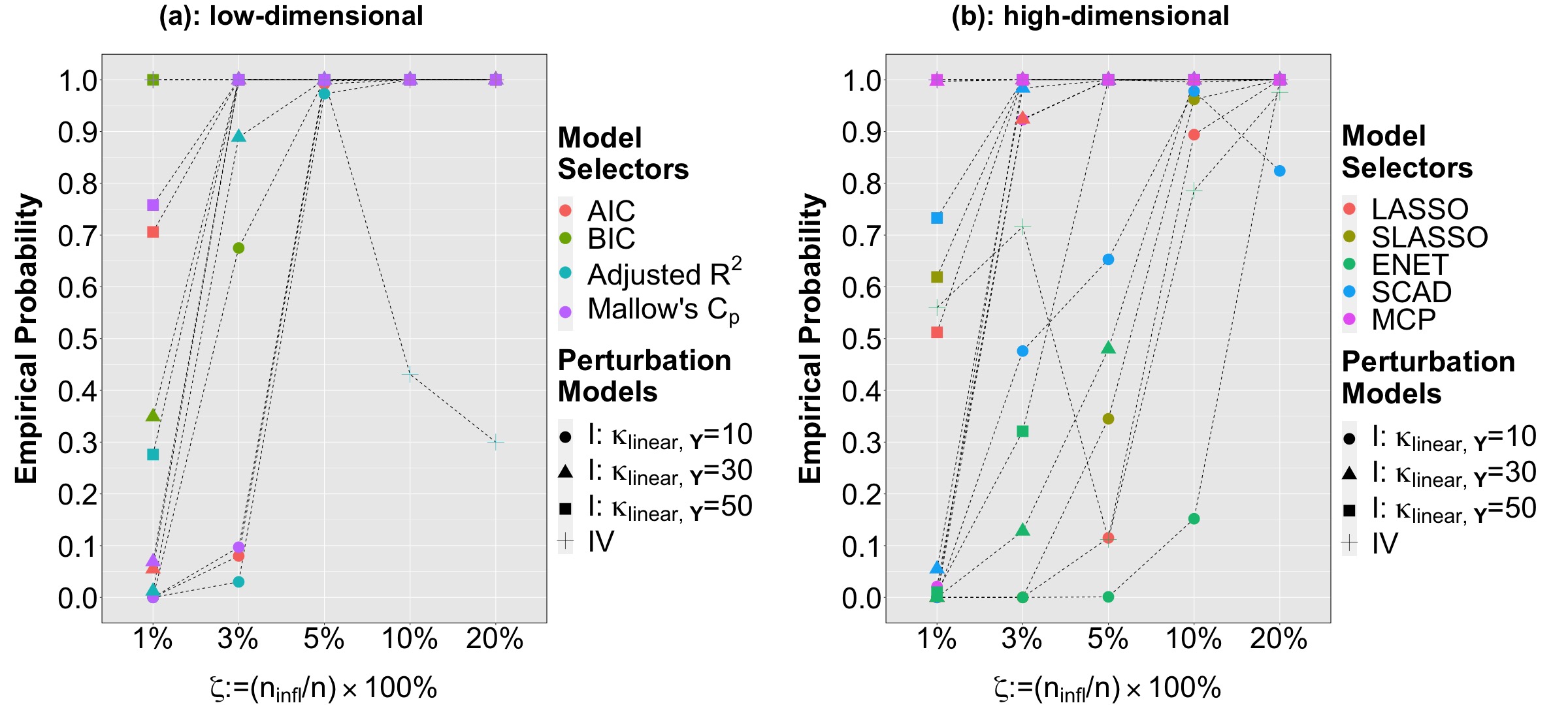
Figure 1: Empirical probability of selecting an incorrect submodel based on the contaminated dataset under $(n,p)$= (a) (100,20), and (b) (100,1000). $n_{\text{infl}}$ is the number of influential observations. Details of data generation and perturbation models are given in Section 1 of the Supplementary Materials.

To gain tangible insights into the pitfalls of ignoring observations exerting disproportionate influence on variable selection, a simulated example is given below in Figure 1 with details provided in Section 1 of the Supplementary Materials, schematically illustrating the non-negligible empirical probability of selecting an incorrect submodel based on the full, contaminated dataset. Thus, given the importance and ubiquity of stochastic variable selection, it is necessary and indeed in practitioners’ best interest, to identify observations influencing the choice of a submodel.

Despite its importance, studies on influential diagnostics in model and variable selection is relatively scarce. In the low-dimensional setting, Leger & Altman (1993) pioneered the study by introducing a variant of Cook’s distance (Cook, 1977) incorporating the randomness of model selection for detection purposes. Recently, in the high-dimensional setting, Rajaratnam et al. (2019) proposed and analyzed a diagnostic measure, known as the difference in model selection (DF(LASSO)), to directly quantify the influence of a single point on variable selection via LASSO. In addition, Zhao et al. (2013) studied the so-called high-dimensional influence measure (HIM), capturing the influence of a single observation on the marginal correlation between the response and predictors. The versatility of this measure is then verified on variable selection via simulated and real data studies. This work is extended in Zhao et al. (2015) and Zhao et al. (2019) to detect multiple influential points, leading to the so-called multiple influential point (MIP) detection procedure. Yet, the aforementioned literature falls short on two different fronts:

1. Limitation to detect multiple influential points: the presence of several influential points in a real dataset is common (Hampel et al., 1986). Two major challenges in detecting them are the so-called “masking” and “swamping” effects (Hadi & Simonoff, 1993). Masking is a phenomenon where an influential point is hidden due the presence of other influential cases. Swamping occurs when a non-influential point is falsely labeled as influential. Indeed, under-performance in mitigating them and accurately capturing multiple influential points is seen from the simulated study in Section 4 for both DF(LASSO) and MIP.

2. Restrictive settings: first, as described later in the paper, one claim in developing the DF(LASSO) is not substantiated, jeopardizing its logical legitimacy. Second, the theoretical framework of the DF(LASSO) is only developed for LASSO. Its applicability to other model selectors is yet to be studied. Third, the foregoing works all assume linear regression models. Few studies are conducted for the generalized linear models (GLM).

This manuscript aims at filling the aforementioned gaps and contributes to influential diagnosis on variable selection in five aspects. First, upon characterizing influential points in assessing variable selection, we introduce the notion of sensitivity of model selectors, and draw connections with statistical concepts such as breakdown points and selection consistency. Second, we consolidate the diagnostic measure of Rajaratnam et al. (2019) in Theorem 1 and Corollary 1 by bridging a missing step in its original theoretical development. Third, a generalized version accommodating universal model selectors is then proposed and the corresponding asymptotic distribution is determined in Theorem 2. The main building blocks of our approach in establishing the large sample distribution of our proposed method are the preservation of exchangeability (Commenges, 2003) and characterization of a sequence of arbitrarily dependent events by its exchangeable counterpart (Galambos, 1973). Fourth, upon integrating a high-dimensional clustering procedure into our framework, we propose a novel detection procedure, known as the clustering-based MIP (ClusMIP), that is capable of identifying multiple influential observations. Lastly, we compare our proposal with competing procedures via comprehensive simulated and real data studies. This enables the analysis of strengths and limitations of different procedures, and assessment of sensitivities of model selectors under consideration.

The rest of this manuscript is organized as follows: in Section 2, we characterize and define influential observations on variable selection. Section 3 begins with a survey of the aforementioned HIM and DF(LASSO) approaches for single influential point detection. We then present our generalized version of DF(LASSO) accompanied by the study of its asymptotic properties. We next discuss the MIP and our newly proposed ClusMIP method to detection multiple influential points. Section 4 contains an intensive simulation study, followed by analysis of a real dataset extracted from Lindquist et al. (2017) on the neurologic signature of physical pain in Section 5. Conclusions are given in Section 6.

Notation

Let $\text{Y}\in\mathbb{R}$ be the response variable and ${x}_{j}\in\mathbb{R},\,j=1,...,p$, be the predictors. Let $\textbf{Y}=(\text{Y}_{1},...,\text{Y}_{n})^{\top}\in\mathbb{R}^{n}$ be the response vector and $\textbf{X}=(\textbf{X}_{1},...,\textbf{X}_{n})^{\top}\in\mathbb{R}^{n\times p}$, where $\textbf{X}_{i}=(\text{X}_{i1},...,\text{X}_{ip})^{\top}\in\mathbb{R}^{p}$, $i=1,...,n$, be the $n\times p$ design matrix. Then, the $i^{\text{th}}$ observation or point of full dataset $\textbf{Z}\coloneqq(\textbf{Y},\textbf{X})$ is $\text{Z}_{i}\coloneqq(\text{Y}_{i},\textbf{X}_{i}^{\top})^{\top}\in\mathbb{R}^{p+1}$, $i=1,..,n$. Moreover, we abbreviate an arbitrary sequence of random variables or real values $a_{1},...,a_{n}$ by $a_{[n]}$.

A linear regression model with i.i.d. errors is defined as

$$\text{Y}_{i}=\textbf{X}_{i}^{\top}\boldsymbol{\beta}+\epsilon_{i},\ i=1,...,n,$$ (1)

where $\boldsymbol{\beta}=(\beta_{1},...,\beta_{p})^{\top}\in\mathbb{R}^{p}$ is the true regression coefficient, and $\epsilon_{i}\sim N(0,\sigma^{2})$ for some $\sigma^{2}>0$. Moreover, the $\epsilon_{i}$’s are independent of X.

2 Assessing Inf luence on Variable Selection

We now characterize and formally define the concept of influential observations on variable selection. It is critical to first recognize that observations influencing the choice of a submodel can only be legitimately understood within a stochastic framework due to the data-dependent nature of model selection. Moreover, due to distinctive model selection criteria, especially different penalty functions of regularized variable selection methods for high-dimensional data, contrasting sets of predictors could be chosen by different model selectors. As such, it is reasonable to conjecture that the extent to which model selectors are perturbed by influential points in terms of selection consistency properties, including model selection consistency (Fan & Lv, 2010) and sign consistency (Zhao & Yu, 2006), varies for different selection procedures. An implication is that influential observations in our context are specific to model selectors, and the same detection procedure as a function of different model selectors may well lead to the detection of distinctive sets of influential points.

In fact, the degree to which a model selector is prone to contamination can be termed as its functional sensitivity to influential observations. This concept can be understood as the percentage of data corruption permitted while fulfilling consistent selection properties. The significance of such sensitivity depends on the dichotomous intents of statistical operations, namely the diagnosis for contaminated data and consistent model selection. For diagnostic purposes, a model selector that is more sensitive to influential points may better facilitate their detection. On the other hand, the later objective of selection consistency underscores the resistance to contamination, which is closely linked to the notion of robustness of an estimator. Under this scenario, functional sensitivity philosophically aligns with the so-called breakdown point (Hampel, 1971; Donoho, 1982) in robust statistics, which is the fraction of data allowed to be perturbed without invalidating the estimation consistency.

From the foregoing discussion, influential points on variable selection can be defined as:

Definition 1.

Influential Observations on Variable Selection. Observations indexed by $\text{I}_{\text{infl}}\subseteq\{1,...,n\}\in\mathcal{P}(\{1,...,n\})$ are called influential observations on variable selection if and only if for each $i\in\text{I}_{\text{infl}}$, $\widehat{\textbf{M}}_{n}\big{(}\textbf{Z}^{\big{(}\{i\}\cup\text{I}_{\text{infl}}^{\mathsf{c}}\big{)}}\big{)}\neq\widehat{\textbf{M}}_{n}\big{(}\textbf{Z}^{\big{(}\text{I}_{\text{infl}}^{\mathsf{c}}\big{)}}\big{)}$, where $\widehat{\textbf{M}}_{n}$ is model selector, which is a measurable function from the data to the space of all possible full-ranked submodels, $\textbf{Z}^{S}$ denotes the data with rows indexed by the set $S$ and $\text{I}_{\text{infl}}^{\mathsf{c}}=\{1,...,n\}\setminus\text{I}_{\text{infl}}$.

Having characterized and formally defined influential observations on variable selection, we next discuss methodological developments for detecting them.

3 Methodology

In this section, we present high-dimensional methods for detecting a single and multiple influential observations in Sections 3.1 and 3.2, respectively.

3.1 Single Inf luential Observation Detection

We begin with a concise review of the HIM and DF(LASSO) in Sections 3.1.1 and 3.1.2, respectively. In Section 3.1.3, two theoretical limitations of DF(LASSO) are addressed, followed by the proposal of a generalized version and study of its asymptotic properties.

3.1.1 High-dimensional Inf luence Measure (HIM)

Based on the linear regression model (1), Zhao et al. (2013) proposed a non-parametric, model-free and theoretically justified diagnostic measure capable of indirectly assessing the influence of a single observation on variable selection for high-dimensional data. Known as the high-dimensional influence measure (HIM), this metric is formulated on the leave-one-out basis and is designed to quantify the contribution of each individual observation to the marginal correlation between the response variable and all the predictors. An observation with excessively large marginal correlation is deemed influential. To compute the HIM, we first calibrate the influence of the $i^{\text{th}}$ observation on the marginal correlation between the response variable Y and $j^{\text{th}}$ predictor $x_{j}$ by calculating its sample estimate $\widehat{\rho}_{j}^{(i)}=\sum_{k=1,k\neq i}^{n}\big{\{}(\text{X}_{kj}-\widehat{\mu}_{xj}^{(i)})(\text{Y}_{k}-\widehat{\mu}_{y}^{(i)})\big{\}}/\big{\{}(n-1)\widehat{\sigma}_{xj}^{(i)}\widehat{\sigma}_{y}^{(i)}\big{\}}$, $j=1,...,p$ and $i=1,...,n$, where $\widehat{\mu}_{xj}^{(i)}=\sum_{k=1,k\neq i}^{n}\text{X}_{kj}/n$, $\widehat{\mu}_{y}^{(i)}=\sum_{k=1,k\neq i}^{n}\text{Y}_{k}/n$, $\big{(}\widehat{\sigma}_{xj}^{(i)}\big{)}^{2}=\sum_{k=1,k\neq i}^{n}(\text{X}_{kj}-\widehat{\mu}_{xj}^{(i)})^{2}/(n-1)$, and $\big{(}\widehat{\sigma}_{y}^{(i)}\big{)}^{2}=\sum_{k=1,k\neq i}^{n}(\text{Y}_{k}-\widehat{\mu}_{y}^{(i)})^{2}/(n-1)$. Then, upon aggregating and averaging over all $p$ predictors, the HIM for the $i^{\text{th}}$ observation is given by $D_{i}=\sum_{j=1}^{p}\big{(}\widehat{\rho}_{j}-\widehat{\rho}_{j}^{(i)}\big{)}^{2}/p,\ i=1,...,n$, where $\widehat{\rho}_{j}^{(i)}$ is given above and $\widehat{\rho}_{j}$ is its counterpart computed based on the full dataset. Under certain conditions (ibid., Conditions C.1 - C.4, Section 2.3), Zhao et al. (2013) establish that in the absence of influential points, $n^{2}D_{i}\rightarrow\chi^{2}(1)\ \text{as}\ \text{min}(n,p)\rightarrow\infty,\ i=1,...,n$, where $\chi^{2}(1)$ is the chi-squares distribution with one degree of freedom. Thus, the scaled percentile of $\chi^{2}(1)$ can be used as a threshold to pinpoint influential observations. The authors then demonstrate the potential to extend their framework to GLM, yet remarking that the above asymptotic distributional property may not hold. The effectiveness of this method in assessing influence on variable selection is further validated via simulated studies.

Despite advantages including computational simplicity and sound theoretical justification, there are limitations of the HIM approach. First, since it is primarily proposed under the linear regression model, its effectiveness when the response variable is nonlinearly correlated with the predictors is ambiguous. Second, when $p$ is close to $n$, spurious correlation may exist between the response variable and predictors leading to unreliable variable selection, an undesirable phenomenon known as the Freedman’s paradox (Freedman, 1983) which persists in high-dimensional settings (Fan et al., 2014). Thus, adopting marginal correlation to evaluate influence on variable selection may be inappropriate. Third, the HIM approach is independent of model selector, thus providing no insights of the sensitivity of a model selector in spite of the fact that it is not intended to perform such function.

3.1.2 Difference in Model Selection Measured by LASSO (DF(LASSO))

In comparison with the indirect approach by Zhao et al. (2013), under (1), Rajaratnam et al. (2019) formulated the so-called difference in model selection (DF(LASSO)) measure to directly gauge the influence of a single point on the submodel selected by LASSO. Similar to the HIM, the DF(LASSO) also hinges on the leave-one-out scheme and is defined by

$$\iota_{i}=\frac{\delta_{i}-\mathbb{E}(\delta_{i})}{\sqrt{\mathrm{Var}(\delta_{i})}},\ i=1,...n,$$ (2)

where

$$\delta_{i}=\sum_{j=1}^{p}\big{\lvert}\mathbbm{1}(\widehat{\beta}_{\text{LASSO},j}=0)-\mathbbm{1}(\widehat{\beta}^{(i)}_{\text{LASSO},j}=0)\big{\rvert}.$$ (3)

Here, $\mathbbm{1}(\cdot)$ is the indicator function, $\widehat{\beta}_{\text{LASSO},j}$ and $\widehat{\beta}^{(i)}_{\text{LASSO},j}$ respectively denote the $j^{\text{th}}$ component of the LASSO estimates obtained from the full dataset and reduced dataset with $i^{\text{th}}$ observation removed. Then, assuming $\sum_{j=1}^{p}\mathbbm{1}(\beta_{j}=0)\rightarrow\infty$, the authors show that

$$\frac{\Delta-\mathbb{E}(\Delta)}{\sqrt{\mathrm{Var}(\Delta)}}\rightarrow N(0,1)\ \text{as}\ \text{min}(n,p)\rightarrow\infty,$$ (4)

where $\Delta=\sum_{j=1}^{p}\big{\lvert}\mathbbm{1}(\widehat{\beta}_{\text{LASSO},j}=0)-\mathbbm{1}(\beta_{j}=0)\big{\rvert}$ and $N(0,1)$ is a standard Gaussian.

In practice, the sample mean and variance of the $\delta_{i}$’s in (3) are suggested to estimate $\mathbb{E}(\delta_{i})$ and $\mathrm{Var}(\delta_{i})$ in (2). For diagnosis, an observation $i$ with $\lvert\iota_{i}\rvert\geq 2$ is considered influential based on the asymptotic Gaussian approximation in (4). From the formulation of the $\delta_{i}$’s, we see that they play central roles in the assessment as they directly quantify the fluctuation in model selection. Moreover, the comparative magnitude of each $\delta_{i}$ in relation to others, rather than its absolute scale, is more important for decision making. In other words, $\delta_{i}$’s shall be viewed from a collective angle to ascertain the nature of any individual observation. Indeed, this interpretation underpins an important perspective that every individual point is influential on variable selection, yet some may be more influential than the others.

Comparing the DF(LASSO) with the HIM, we observe that in terms of methdological philosophies, while the DF(LASSO) explicitly captures the deviation in the selected submodels via changes in the sparsity of the LASSO regression coefficients obtained from the full and reduced datasets, the HIM takes advantage of the marginal correlation as the primary diagnosis instrument, leading to influence induced in an implicit, latent manner. On the computational front, the DF(LASSO) requires fitting $n+1$ models, while no such process is required for the HIM. Thus, the HIM is more computational efficient.

Apart from the above characteristics, there are limitations of the DF(LASSO) framework. First, in establishing (4), the authors recommend using the sample mean and variance of $\delta_{[n]}$ to estimate $\mathbb{E}(\delta_{i})$ and $\mathrm{Var}(\delta_{i})$, which is not theoretically substantiated. Second, the asymptotic normality in (4) is specifically derived for the LASSO estimator. The applicability of this theoretical framework to other model selectors is yet to be established.

3.1.3 Generalized Difference in Model Selection Measure (GDF)

We now address two limitations associated with the DF(LASSO) approach, namely: (i) the legitimacy of estimating $\mathbb{E}(\delta_{i})$ and $\mathrm{Var}(\delta_{i})$ by the sample mean and variance, and (ii) applicability to extend the framework to other model selectors. To achieve that, we note that $\delta_{[n]}$ is a sequence of dependent random variables and each $\delta_{i}$ is a sum of correlated Bernoulli random variables, where both dependence structures have no tractable forms.

To address the first issue regarding the eligibility of estimating $\mathbb{E}(\delta_{i})$ and $\mathrm{Var}(\delta_{i})$ by the corresponding sample mean and variance, we first focus on the finite-sample property of $\delta_{[n]}$ and bridge the gap between this sequence and the characteristic of the original dataset. With Theorem 1 reported below, we show that $\delta_{[n]}$ is exchangeable and thus identically distributed. The proof of Theorem 1 is given in Section 2 of the Supplementary Materials.

Theorem 1.

Suppose that the dataset $\textbf{Z}=(\text{Z}_{1},...,\text{Z}_{n})^{\top}$, where $\text{Z}_{i}=(\text{Y}_{i},\textbf{X}_{i}^{\top})^{\top}\in\mathbb{R}^{p+1},\ i=1,...n$, has i.i.d. rows. Then, the sequence of non-negative, discrete diagnostic measures $\delta_{[n]}$ defined in (3) is exchangeable and thus marginally identically distributed.

From Theorem 1, we next provide two relevant results of an exchangeable sequence of random variables in Corollary 1, which are the consistency of the empirical cumulative distribution function (ECDF) and strong law of large numbers (SLLN). The combined statements further strengthen the theoretical basis for estimating $\mathbb{E}(\delta_{i})$ and $\mathrm{Var}(\delta_{i})$ by the sample mean and variance. Its proof is given in Section 3 of the Supplementary Materials.

Corollary 1.

Let $\delta_{[n]}$ in (3) be defined on a probability space $(\Omega,\mathcal{F},\mathbb{P})$, and let $\mathcal{F}_{\infty}$ be its tail $\sigma$-algebra. Moreover, let $\bar{\delta}\coloneqq\frac{1}{n}\sum_{i=1}^{n}\delta_{i}$. Then, as $n\rightarrow\infty$, we have

1. Uniform Convergence of ECDF: $\sup_{x\in\mathbb{R}}|\widehat{F}_{n}-F|\xrightarrow{\text{a.s.}}0$, where $\widehat{F}_{n}(x)=\sum_{i=1}^{n}\mathbbm{1}(\delta_{i}\leq x)$, $x\in\mathbb{R}$ and $F$ is the true cumulative distribution function (CDF) of $\delta_{[n]}$. In particular, the discontinuity of the limiting CDF $F$ is permitted.

2. SLLN: $\frac{1}{n}\sum_{i=1}^{n}\delta_{i}\xrightarrow{\text{a.s.}}\mathbb{E}(\delta_{i}|\mathcal{F}_{\infty})$ and $\frac{1}{n}\sum_{i=1}^{n}(\delta_{i}-\bar{\delta})^{2}\xrightarrow{\text{a.s.}}\mathrm{Var}(\delta_{i}|\mathcal{F}_{\infty})$.

To address the second issue on the applicability of the DF(LASSO) framework to other model selectors, it is crucial to recognize that the crux of the problem indeed lies in ascertaining the finite- or large-sample distribution of $\tau_{[n]}$, which is the counterpart of $\delta_{[n]}$ in (3) without model selector restriction and is therefore component-wise defined by

$$\tau_{i}=\sum_{j=1}^{p}\xi_{i,j}\ \text{and}\ \xi_{i,j}\coloneqq\lvert\mathbbm{1}(\widehat{\beta}_{j}=0)-\mathbbm{1}(\widehat{\beta}^{(i)}_{j}=0)\rvert,i=1,...,n,$$ (5)

where $\widehat{\beta}_{j}$ and $\widehat{\beta}^{(i)}_{j}$ are the $j^{\text{th}}$ components of a generic sparse regression coefficient estimate obtained based on the full and reduced data with the $i^{\text{th}}$ observation removed, respectively. As such, $\tau_{i}$ in (5) is referred to as the generalized difference in model selection (GDF) measure in the sequel. To understand the distributional properties of $\tau_{i}$, both parametric and non-parametric approaches can provide reliable and theoretically appropriate approximations. In this article, we specifically focus on one such avenue by theoretically justifying the central limit theorem (CLT) for each $\tau_{i}$ via an approach distinctive from Rajaratnam et al. (2019). Such proposition is further strengthened by additional plausibility arguments via an array of unique angles.

To verify the CLT for $\tau_{i}$, we bridge the theoretical hiatus in Rajaratnam et al. (2019) for generic model selectors through the work of Galambos (1973), which bypasses the challenge in handling the intractable dependence among its summands $\xi_{i,j}$. Specifically, it is shown [ibid., Theorem 1] that for an arbitrary sequence of events, there always exists a sequence of exchangeable events such that the respective sums are equally distributed in finite sample. This implies that $\tau_{i}$ in (5), the sum of dependent indicators $\xi_{i,j},j=1,...,p$, is identically distributed as the sum of a sequence of exchangeable Bernoulli random variables. Toward that end, the regular (Klass & Teicher, 1987) and empirical (Hahn & Zhang, 1998) CLT for an exchangeable sequence of random variables collectively facilitate the derivation of the following assertion, where its proof is available in Section 4 of the Supplementary Materials:

Theorem 2.

Let $\tau_{i}$ be defined as in (5). If there exists sequences $a_{p}\in\mathbb{R}$, $0<b_{p}\rightarrow\infty$ and $\epsilon_{p}\downarrow 0$ such that as $p\rightarrow\infty$, the following conditions hold: (C.1) $p\cdot\mathbb{P}^{\omega}(\lvert\Xi_{1}\rvert>\epsilon_{p}b_{p})\rightarrow 0$, where $\mathbb{P}^{\omega}$ is a regular conditional distribution for $\xi_{i,j}$ given $\mathcal{F}_{\infty}$, the tail $\sigma$-algebra generated by $\xi_{i,j}$, such that for each $\omega\in\Omega$, the so-called mixands $\Xi_{k}$, $k=1,...,p$, are i.i.d.; (C.2) $b_{p}/\sqrt{p}$ is slowly varying with $v_{p}(\omega)/b_{p}\rightarrow 1$ and $(a_{p}(\omega)-a_{p})/b_{p}\rightarrow 0$, where $a_{p}(\omega)=p\cdot\mathbb{E}\Xi_{1}\mathbbm{1}(\lvert\Xi_{1}\rvert\leq\epsilon_{p}b_{p})$ and $v_{p}^{2}(\omega)=p\cdot\big{(}\mathbb{E}(\Xi_{1}^{2}\mathbbm{1}(\lvert\Xi_{1}\rvert\leq\epsilon_{p}b_{p}))-\big{(}\mathbb{E}\Xi_{1}\mathbbm{1}(\lvert\Xi_{1}\rvert\leq\epsilon_{p}b_{p})\big{)}^{2}\big{)}$, then,

$$\frac{\tau_{i}-\bar{\xi}}{\sigma_{\xi}}\rightarrow N(0,1)\ \text{as}\ p\rightarrow\infty,$$ (6)

where $\bar{\xi}$ and $\sigma^{2}_{\xi}$ are the sample mean and variance of the binary sequence $\xi_{i,j}$, $j=1,...,p$.

In practice, since $\tau_{[n]}$ itself is exchangeable by Theorem 1 and with further justification from Corollary 1, $\bar{\xi}$ and $V(\xi)$ can be reasonably supplanted by the sample mean ($\bar{\tau}$) and variance ($\sigma^{2}_{\tau}$) of $\tau_{[n]}$ for large $n$. From (6), at a given nominal level $\alpha\in(0,1)$, the $100\cdot(1-\alpha/2)^{\text{th}}$ percentile of $N(0,1)$ is a valid threshold such that an observation with an absolute magnitude of the standardized $\tau_{i}$ exceeding that cut-off is deemed influential. On the other hand, to test the two-sided hypothesis that the $i^{\text{th}}$ point is not influential, the $p$-value is $2\cdot\mathbb{P}(N(0,1)>(\tau_{i}-\bar{\tau})/\sigma_{\tau})$. Such scheme to identify a single influential observation via the GDF measure is summarized in Algorithm 1.

Algorithm 1 Single Influential Point Detection via the GDF Measure (5)

1:Compute the generic, sparse regression coefficient estimate $\widehat{\boldsymbol{\beta}}$ from the full dataset.

2:Compute $\widehat{\boldsymbol{\beta}}^{(i)}$, $i=1,...,n$, the regression coefficients based on the leave-one-out scheme.

3:Compute $\tau_{i}$, $i=1,...,n$, the associated sample mean ($\bar{\tau}$) and variance ($\sigma^{2}_{\tau}$). Here, $\tau_{i}=\sum_{j=1}^{p}\lvert\mathbbm{1}(\widehat{\beta}_{j}=0)-\mathbbm{1}(\widehat{\beta}^{(i)}_{j}=0)\rvert$, where $\widehat{\beta}_{j}$ and $\widehat{\beta}^{(i)}_{j}$ are obtained from Steps 1 and 2.

4:Given a nominal level $\alpha\in(0,1)$, the individual $k^{\text{th}}$ observation is influential if $\rvert(\tau_{k}-\bar{\tau})/\sigma_{\tau}|>\gamma_{\alpha}$, where $\gamma_{\alpha}$ is the $100\cdot(1-\alpha/2)^{\text{th}}$ percentile of a standard normal $N(0,1)$. To test hypothesis that $k^{\text{th}}$ point is not influential, the $p$-value is $2\cdot\mathbb{P}(N(0,1)>(\tau_{k}-\bar{\tau})/\sigma_{\tau})$.

To further reinforce (6), by de Finetti’s Theorem (de Finetti, 1931), an exchangeable sequence of random variables can be essentially treated as an i.i.d. sequence given its data generating mechanism. Moreover, Aldous (1977) and references therein further explain that a sequence of arbitrarily dependent random variables, including an exchangeable sequence, contains a subsequence sharing analogous properties of its i.i.d. counterpart. Thus, these discussions offer extra plausibility evidence supporting the SLLN and CLT of $\delta_{[n]}$ and $\tau_{[n]}$.

3.2 Multiple Inf luential Observations Detection

To detect multiple influential observations, we first review the multiple influential point (MIP) detection algorithm by Zhao et al. (2019) in Section 3.2.1, which is an extension of the HIM procedure discussed in Section 3.1.1. This is followed by the proposal of our clustering-based multiple influential point (ClusMIP) detection method in Section 3.2.2.

3.2.1 Multiple Inf luential Point (MIP) Detection Procedure

The leave-one-out basis of the HIM approach implies that it may not be effective in capturing multiple influential points. To remedy this issue, Zhao et al. (2019) propose the MIP method via integrating the so-called random-group-deletion (RGD) scheme into the HIM framework. Based on this, two HIM-based statistics are subsequently formulated to overcome both masking and swamping effects in detecting multiple influential observations.

To have a proper understanding of this procedure, we first explain the philosophy underlying the RGD algorithm, which is provided in Section 5 of the Supplementary Materials. The RDG scheme centers on seeking and subsequently attaching a clean subset of data to every single point, of which refinement is conducted based on the combined dataset. To be more precise, for each observation $i$, $m$ samples indexed by $A_{1},...,A_{m}$ are drawn uniformly and randomly from the remaining portion of the data. When $m$ is sufficiently large, there is a high probability that the subset $\{\text{Z}_{r}:r\in A_{j}\}$ is clean for some $j\in\{1,...,m\}$. Thus, if $i^{\text{th}}$ observation is contaminated, it would be the sole influential point in the merged subset $\{\text{Z}_{r}:r\in A_{j}\cup\{i\}\}$. Thus, further assessment can be carried out on this combined dataset.

Toward that end, for each $i$, two HIM-based statistics $\text{T}_{\text{min},i,m}$ and $\text{T}_{\text{max},i,m}$ are then constructed, which are respectively defined by $\text{T}_{\text{min},i,m}=\arg\!\min_{1\leq j\leq m}n_{\text{sub}}^{2}D_{j,i}$ and $\text{T}_{\text{max},i,m}=\mathop{\mathrm{argmax}}_{1\leq j\leq m}n_{\text{sub}}^{2}D_{j,i}$, where $D_{j,i}=\sum_{k=1}^{p}\big{(}\widehat{\rho}_{k}^{(A_{j}\cup\{i\})}-\widehat{\rho}_{k}^{(A_{j}}\big{)}^{2}/p$. Here, $\widehat{\rho}_{k}^{(A_{j}\cup\{i\})}$ and $\widehat{\rho}_{k}^{(A_{j})}$ are the sample marginal correlations between the response Y and $k^{\text{th}}$ predictor $x_{k}$ based on $\{\text{Z}_{r}:r\in\{A_{j}\cup\{i\}\}\}$ and $\{\text{Z}_{r}:r\in A_{j}\}$. The authors then establish that they are both asymptotically $\chi^{2}(1)$ and indeed complement each other: $\text{T}_{\text{min},i,m}$ tends to select conspicuously influential points. Thus, it is effective in overcoming the swamping effect. However, it may be conservative so that true influential points may be neglected. In contrast, $\text{T}_{\text{max},i,m}$ is powerful to counter the masking effect. Yet, it may be inordinately aggressive so that clean ones may be falsely chosen. Therefore, combining the strengths of both $\text{T}_{\text{min},i,m}$ and $\text{T}_{\text{max},i,m}$ leads to the MIP detection procedure provided in Section 6 of the Supplementary Materials. In practice, the MIP algorithm is implemented in the $\tt{R}$ package $\tt{MIP}$.

3.2.2 Clustering-based MIP (ClusMIP) Detection Procedure

Motivated by Zhao et al. (2015, 2019), one apparent solution to detect multiple influential observations specifically on variable selection is to integrate the aforementioned RGD scheme into the GDF framework (Section 3.1.3), leading to the proposal of the RGD-based GDF (RGDF) procedure provided in Section 7 of the Supplementary Material.

Indeed, examination of both the MIP and RGDF procedures shows that they consist of two broad stages, the preliminary filtering and secondary refining phases. The main purpose of the filtering stage is to obtain an estimate of the potentially influential points. Then, this set is refined to remove false selections, leading to the final estimate of influential points. In fact, this agrees with our perspective of influential points on variable selection provided in Definition 1, where the complete dataset is separated into clean and contaminated parts so that the concept of an influential point can be unambiguously understood and formalized.

On the other hand, it is crucial to note that the detection outcomes of the MIP and RGDF procedures largely hinge on the accuracy (effectiveness) and the accompanying computational cost (efficiency) of the filtering stage in producing a reliable set of influential points. The MIP can be deemed both effective and efficient since the computations of $\text{T}_{\text{min},i,m}$ and $\text{T}_{\text{max},i,m}$ are model-free. Yet, in our case, for a fixed number of random draws $m$ with $n_{\text{size}}$ being the cardinality of each random sample, a maximum of $nm(n_{\text{size}}+2)$ final fitted models are obtained. This is computationally expensive even if $n$, $m$ and $n_{\text{size}}$ are moderate. Thus, efficiency could be severely compromised in the RGDF framework when iterative model fitting is involved to assess influence on variable selection.

To alleviate the exorbitant computational costs, instead of the foregoing RGD strategy, we incorporate an appropriate high-dimensional clustering procedure for initially partitioning the complete dataset into approximately clean ($\widehat{\text{S}}_{\text{clean}}$) and influential ($\widehat{\text{S}}_{\text{infl}}$) proportions. Then, each observation $k$ in $\widehat{\text{S}}_{\text{infl}}$ is further assessed based on the sole subset of the data indexed by $\{k\}\cup\widehat{\text{S}}_{\text{clean}}$ via Algorithm 1 which is proposed for detecting a single influential observation through the GDF measure (5). In addition, to simultaneously test the $\rvert\widehat{\text{S}}_{\text{infl}}\lvert$ hypotheses that the $k^{\text{th}}$ observation is not influential, $k\in\widehat{\text{S}}_{\text{infl}}$, the procedure of Benjamini & Hochberg (1995) is adopted to address the multiple testing issue. This leads to our ClusMIP algorithm summarized in Algorithm 2.

Algorithm 2 Clustering-based Multiple Influential Point Detection (ClusMIP)

1:Partition the dataset into the potentially influential ($\widehat{\text{S}}_{\text{infl}}$) and clean ($\widehat{\text{S}}_{\text{clean}}$) proportions via an appropriate high-dimensional clustering procedure, where $\lvert\widehat{\text{S}}_{\text{infl}}\rvert<|\widehat{\text{S}}_{\text{clean}}\rvert$.

2:Given a nominal level $\alpha\in(0,1)$, the final estimated influential observations set is $\widehat{\text{I}}_{\text{infl}}=\{j\in\widehat{\text{S}}_{\text{infl}}:\lvert(\tau_{j}-\tilde{\tau}_{j})/\tilde{\sigma}_{\tau_{j}}\rvert>\gamma_{\alpha}\}$, where for each $j\in\widehat{\text{S}}_{\text{infl}}$, $\tau_{j}$ is computed from subset indexed by $\{j\}\cup\widehat{\text{S}}_{\text{clean}}$, and $\tilde{\tau}_{j}$ and $\tilde{\sigma}_{\tau_{j}}$ are the sample mean and variance of $\{\tau_{k}:k\in\{j\}\cup\widehat{\text{S}}_{\text{clean}}\}$. To simultaneously test hypotheses that $k^{\text{th}}$ point is not influential, $k\in\widehat{\text{S}}_{\text{infl}}$, procedure of Benjamini & Hochberg (1995) is adopted.

The intent and accompanying advantage of integrating a clustering operation is four-fold. First, it mitigates the computational requirement via offering a fast and conveniently implementable solution. Second, the heterogeneity ingrained in the data, which contributes to the discrepancy in variable selection, could be captured by the resulting partition outcomes. Third, despite being potentially inaccurate, such partition outcomes are then refined in the second stage via further assessment through the GDF measure, safeguarding the detection accuracy. Lastly, as shown in Theorem 3 and verified in the simulated study (Section 4), the integration of such clustering controls the false positive rate (FPR) at a given false discovery rate (FDR) $\alpha_{0}\in(0,1)$ in any finite sample. Indeed, the FPR diminishes as $\min(n,p)\rightarrow\infty$ if the clustering is strongly consistent in estimating the true cluster centers. Thus, it remains to pinpoint a reasonable high-dimensional clustering candidate.

Toward that end, one possible approach is $K$-means clustering (KC), which minimizes the within-cluster Euclidean distance. Pollard (1981) provides conditions for the strong consistency of the KC, showing that with the correct number of clusters, the cluster centers converge to their true counterparts as $n\rightarrow\infty$ under certain conditions. Yet, this approach is limited on three facets. First, its widely adopted approximating algorithm, known as Lloyd’s algorithm, may not be globally optimal due to its heavy sensitivity to the starting points. Second, the consistency of the KC may not hold under diverging dimension $p\rightarrow\infty$. Third, under such high-dimensional settings, the notion of distance in terms of the $\ell^{p}$ norm may not be meaningful (Beyer et al., 1999). Indeed, it is justified [ibid., Theorem 1] that as $p\rightarrow\infty$, the ratio of the distances in $\ell^{p}$ norm of the nearest and furthest points to a reference point approaches 1, implying that points tend to be uniformly separated in the high-dimensional $\ell^{p}$ space. In fact, this assertion aligns with the geometric characterization of high-dimensional data (Hall et al., 2005), showing that as $p$ increases while $n$ remains fixed, the data tend to cluster at the vertices of a deterministic simplex.

To address the first limitation, an improved choice of the initial values for the KC algorithm is proposed by Arthur & Vassilvitskii (2007), leading to the so-called $K$-means++ algorithm (KC++). In addition, to resolve the challenges brought about by the high dimensionality, two categories of remedial proposals are available in the literature, which are known as the projection-based and regularized clustering. The projection-based scheme is a hybrid technique by first projecting the high-dimensional data onto a low-dimensional space, followed by partition via the KC. Two proposals under this category are the $t$-distributed stochastic neighbor embedding ($t$-SNE) (Hinton & Roweis, 2002) and spectral clustering (Ng et al., 2001), where the projected low-dimensional space for the later work is spanned by eigenvectors of the normalized graph Laplacians. In comparison, the regularized clustering augments a penalty term to the appropriate objective function to obtain estimates of penalized cluster centers. One such approach is called regularized KC (Sun et al., 2012), where a group LASSO penalty term is adopted and strong consistency of cluster centers is established [ibid., Theorem 1] for $p\rightarrow\infty$. These five clustering procedures, including the KC, KC++, $t$-SNE, spectral clustering and regularized KC are empirically compared on all the simulation configurations considered in Section 4. The corresponding graphical illustrations are reported in Section 9 of the Supplementary Materials, where all of them exhibit analogously satisfactory detection of clusters. Indeed, in both finite and diverging dimensions, with a consistent clustering technique that is further refined via the CLT of the GDF measure (5) established in Theorem 2, the FPR of the foregoing ClusMIP algorithm is controlled at a given the FDR which is stated below, where the proof is given in Section 8 of the Supplementary Materials:

Theorem 3.

Suppose that the proportion of the true clean observations is more than 1/2. Then, given the FDR controlled at $\alpha_{0}\in(0,1)$, we have

1. $\mathbb{E}[\text{FPR}(\text{ClusMIP})]\leq\alpha_{0}$ at any finite dimensions $n$ and $p$, and

2. $\mathbb{E}[\text{FPR}(\text{ClusMIP})]\rightarrow 0$ as $\min{(n,p)}\rightarrow\infty$.

where the FPR(ClusMIP) refers to the FPR of the ClusMIP procedure given in Algorithm 2.

4 Simulation Study

We now conduct simulation study to assess and compare the performance of the various detection techniques discussed in Section 3 for high-dimensional data. The details of data generation are provided in Section 4.1, followed by evaluation criteria and implementation details respectively in Sections 4.2 and 4.3. Analysis of results is given in Section 4.4.

4.1 Data Generation

The specifics of data generation are given as follows:

Design Matrices X

Let $(n,p)=(100,1000)$. X follows a multivariate normal distribution, generated as $\textbf{X}\sim\mathcal{N}(\boldsymbol{0},\Sigma(\rho))$, where $\Sigma(\rho)$ is the Toeplitz-type variance-covariance matrix indexed by the correlation coefficient $\rho$, and its $(i,j)$-entry is given by $\Sigma_{i,j}(\rho)=\rho^{|i-j|}$, $i=1,...,p$ and $j=1,...,p$. Here, we consider $\rho=0,0.5$ and $0.8$ so that the corresponding design matrices are denoted by $\textbf{X}_{\text{Tp(0)}}$, $\textbf{X}_{\text{Tp(0.5)}}$ and $\textbf{X}_{\text{Tp(0.8)}}$, respectively.

Influential and Clean Observations

We consider the data generating mechanism via the linear regression model (1). Specifically, we simulate influential and clean observations according to the following two-step procedure: first, generate $n=100$ observations based on (1). Second, generate $n_{\text{infl}}$ points, denoted by $\{\textbf{Z}_{i,\text{infl}}=(\text{Y}_{i,\text{infl}},\textbf{X}_{i,\text{infl}}^{\top})^{\top}\in\mathbb{R}^{1001}:i=1,...,n_{\text{infl}}\}$, according to three perturbation models presented below, where $n_{\text{infl}}$ is the number of influential points. The first $n_{\text{infl}}$ points in the first step are then replaced by $\textbf{Z}_{i,\text{infl}},i=1,..,n_{\text{infl}}$, yielding the heterogeneously contaminated dataset. Here, the three perturbation models respectively introduce contamination to the response vector only, design matrix only and both of them simultaneously. Furthermore, the proportion of contamination $\zeta\coloneqq(n_{\text{infl}}/n)\times 100\%$ is considered to be $5\%,10\%,15\%$ and $20\%$. From this two-step scheme, we next provide data generation specifics for (1), which are also summarized in Section 10.1 of the Supplementary Materials.

Linear Regression Model

The true regression coefficient in (1) is $\boldsymbol{\beta}=\{2,1,1,0,...,0\}^{\top}\in\mathbb{R}^{p}$ and $\sigma^{2}=1$. To generate influential points, we define $i_{\text{linear},\text{max}}=\mathop{\mathrm{argmax}}_{1\leq i\leq n}\text{Y}_{i}$ to facilitate the distinction of them from the clean portion based on the chosen clustering procedure. Then, for $i=1,...,n_{\text{infl}}$, we adapt and modify the settings in Zhao et al. (2013) and propose:

1. Perturbation Model I (Contamination on the Response): $\textbf{X}_{i,\text{infl}}=\textbf{X}_{i}$ and $\text{Y}_{i,\text{infl}}=\text{Y}_{i_{\text{linear},\text{max}}}\\ +\epsilon_{i}+\kappa_{\text{linear},\textbf{Y}}$, where $\epsilon_{i}\sim N(0,1)$ and $\kappa_{\text{linear},\textbf{Y}}\in\{5,10\}$.

2. Perturbation Model II (Contamination on the Predictors): $\text{X}_{ij,\text{infl}}=\text{X}_{ij}+\kappa_{\text{linear},\textbf{X}}\cdot\mathbbm{1}\big{\{}j\in\{1,...,10\}\big{\}}$, $\kappa_{\text{linear},\textbf{X}}\in\{5,10\}$, $\textbf{X}_{i,\text{infl}}=(\text{X}_{i1,\text{infl}},...,\text{X}_{ip,\text{infl}})^{\top}$, and $\text{Y}_{i,\text{infl}}=\text{Y}_{i}$.

3. Perturbation Model III (Contamination on the Response and Predictors): $\text{X}_{ij,\text{infl}}=\\ \text{X}_{i_{\text{linear},\text{max}}j}+0.5\ \kappa_{\text{linear},\textbf{X}}\cdot\mathbbm{1}\big{\{}j\in\{1,...,10\}\big{\}}$, $\textbf{X}_{i,\text{infl}}=(\text{X}_{i1,\text{infl}},...,\text{X}_{ip,\text{infl}})^{\top}$, and $\text{Y}_{i,\text{infl}}=(\textbf{X}_{i,\text{infl}})^{\top}\boldsymbol{\beta}+\epsilon_{i}+\kappa_{\text{linear},\textbf{Y}}$, where $\epsilon_{i}\sim N(0,1)$ and $(\kappa_{\text{linear},\textbf{X}},\kappa_{\text{linear},\textbf{Y}})\in\{(5,5),(10,10)\}$.

4.2 Assessment Metrics

We consider three assessment criteria, which are the power of detection, false positive rate and algorithm running time. Denoted by $\text{Power}_{\text{Detection}(\text{Selector})}$, $\text{FPR}_{\text{Detection}(\text{Selector})}$ and $\text{Time}_{\text{Detection}(\text{Selector})}$, they are defined by

$$\text{Power}_{\text{Detection}(\text{Selector})}=\frac{\sum_{b=1}^{1000}\ \widehat{\text{I}}^{\text{infl}}_{\text{Detection}(\text{Selector}),b}\ \cap\ \{1,...,n_{\text{infl}}\}}{n_{\text{infl}}\times 1000},$$

$$\text{FPR}_{\text{Detection}(\text{Selector})}=\frac{\sum_{b=1}^{1000}\ \widehat{\text{I}}^{\text{infl}}_{\text{Detection}(\text{Selector}),b}\ \cap\ \{n_{\text{infl}}+1,...,n\}}{(n-n_{\text{infl}})\times 1000},\ \text{and}\$$

$$\text{Time}_{\text{Detection}(\text{Selector})}=\frac{\sum_{b=1}^{1000}\ \widehat{\text{T}}_{\text{Detection}(\text{Selector}),b}}{1000},$$

where “Detection(Selector)” specifies the identification procedure “Detection” when a submodel is selected by “Selector”. Moreover, $\widehat{\text{I}}^{\text{infl}}_{\text{Detection}(\text{Selector}),b}$ and $\widehat{\text{T}}_{\text{Detection}(\text{Selector}),b}$ respectively denote the estimated index set of influential observations and execution time (in seconds) for identifying them based on the $b^{\text{th}}$ generated random sample, $b=1,...,1000$.

4.3 Methods, Codes and Implementation

In our simulations, different combinations of detection procedures and model selectors are considered according to the types of data generating mechanisms.

Under the linear regression model (1), we consider three detection procedures: the ClusMIP (Algorithm 2), and the two competing proposals DF(LASSO) and MIP. In case of $\textbf{X}_{\text{Tp(0.5)}}$ and $\textbf{X}_{\text{Tp(0.8)}}$, we combine the ClusMIP with the LASSO, scaled LASSO (SLASSO), elastic net (ENET), SCAD and MCP, while the ENET is excluded in case of $\textbf{X}_{\text{Tp(0)}}$.

In addition, tuning parameter for all the regularized model selectors is selected via the 10-fold cross-validation (CV), unless otherwise specified. A summary of methods and implementation details is provided in Section 10.2 of the Supplementary Materials.

4.4 Simulation Results

Now, we present and analyze selected simulation results classified according to the types of data generating mechanisms and perturbation models, for which distinctive patterns of the three assessment benchmarks presented in Section 4.2 have been recognized. All the simulation diagrammatic results are provided in Section 10.3 of the Supplementary Materials.

Linear Regression Model: Perturbation Model I (Figure 2)

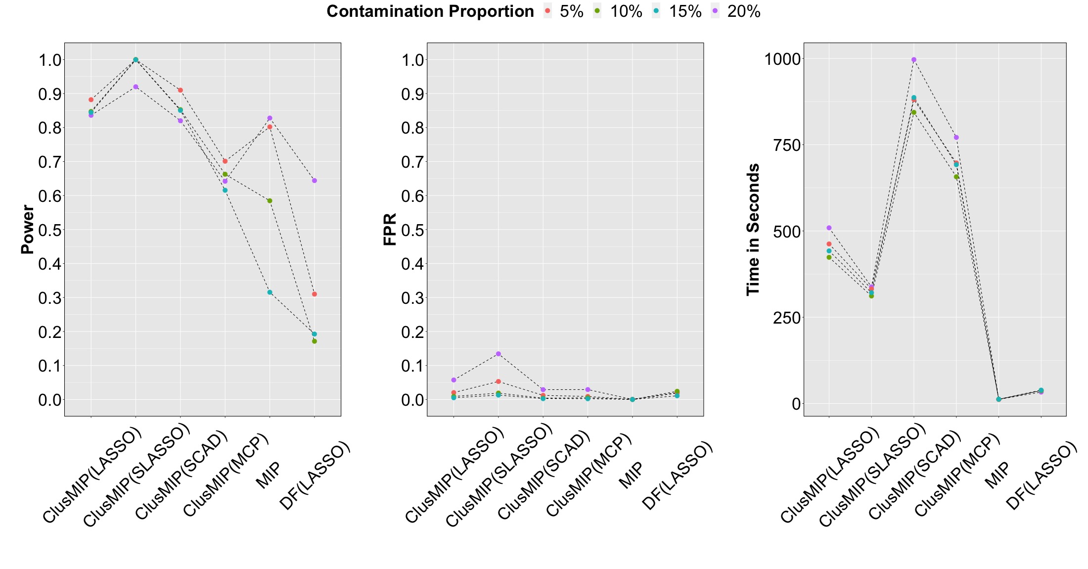
Figure 2: Assessment under the linear regression model, Perturbation Model I, $\kappa_{\text{Linear},\textbf{Y}}=$5 and $\textbf{X}_{\text{Tp(0)}}$.

1. Power: when $\kappa_{\text{Linear},\textbf{Y}}=5$ and $\textbf{X}=\textbf{X}_{\text{Tp(0)}}$, $\text{Power}_{\text{ClusMIP}(\text{LASSO})}$, $\text{Power}_{\text{ClusMIP}(\text{SLASSO})}$ and $\text{Power}_{\text{ClusMIP}(\text{SCAD})}$ are higher than $\text{Power}_{\text{MIP}}$ and $\text{Power}_{\text{DF}(\text{LASSO})}$ for the same contamination proportion $\zeta$. Specifically, $\text{Power}_{\text{ClusMIP}(\text{SLASSO})}$ is the highest, reaching almost 1.00 for all contamination proportions except for $5\%$. In comparison, large variation exists for both $\text{Power}_{\text{MIP}}$ and $\text{Power}_{\text{DF}(\text{LASSO})}$, dropping respectively from 0.83 to 0.32 and 0.64 to 0.19 as $\zeta$ increases. For the remaining simulation configurations, in general we have $\text{Power}_{\text{ClusMIP}(\text{SLASSO})}\approx\text{Power}_{\text{MIP}}\approx 1.00>\big{\{}\text{Power}_{\text{ClusMIP}(\text{LASSO})},\text{Power}_{\text{ClusMIP}(\text{ENET})},\\ \text{Power}_{\text{ClusMIP}(\text{SCAD})},\text{Power}_{\text{ClusMIP}(\text{MCP})}\big{\}}\gg\text{Power}_{\text{DF}(\text{LASSO})}$. Both ClusMIP(SLASSO) and MIP almost capture all the influential points, implying that SLASSO is sensitive to influential points in variable selection, serving as a reasonable candidate for identification purpose. Moreover, detection powers of ClusMIP(LASSO), ClusMIP(ENET), ClusMIP(SCAD) and ClusMIP(MCP) are noticeably lower, ranging between 0.70 and 0.90. In particular, detection powers of ClusMIP(LASSO) and ClusMIP(SCAD) are comparable in magnitude over the same $\zeta$, followed by ClusMIP(ENET) and ClusMIP(MCP). In contrast, $\text{Power}_{\text{DF}(\text{LASSO})}$ is almost always less than 0.4, highlighting its incapability to detect multiple influential observations.

2. FPR: across all the design matrices, perturbation scales and contamination proportions, all procedures exhibit consistently small FPR, ranging between 0 and $5.0\%$ which is less than the nominal level $\alpha=0.05$. This phenomenon justifies Theorem 3 for the ClusMIP procedure and Theorem 4 in Zhao et al. (2019) in controlling the FPR. Specifically, the high-dimensional clustering is effective to separate the clean data from the contaminated portion, limiting the possibility for false identification in the subsequent refinement step. On the other hand, the $\text{FPR}_{\text{ClusMIP(SLASSO)}}$ computed for $\textbf{X}_{\text{Tp(0)}}$, $\kappa_{\text{Linear},\textbf{Y}}=5$ and $\zeta=5\%$ seems to be an outlying case, which attains an elevated level of approximately $15.0\%$.

3. Computation Time: in general, we have $\text{Time}_{\text{MIP}}<\text{Time}_{\text{DF}(\text{LASSO})}\{\text{Time}_{\text{ClusMIP}(\text{LASSO})},\\ \ll\text{Time}_{\text{ClusMIP}(\text{SLASSO})},\text{Time}_{\text{ClusMIP}(\text{SCAD})},\text{Time}_{\text{ClusMIP}(\text{MCP})}\}\ll\text{Time}_{\text{ClusMIP}(\text{ENET})}$. Noticeably, $\text{Time}_{\text{MIP}}$ and $\text{Time}_{\text{DF}(\text{LASSO})}$ are negligible comparing with that of the ClusMIP approach. This is because that the MIP involves no model fitting. Moreover, the authors further remark [Zhao et al. (2019), Theorem 4] that one iteration of their algorithm suffices to capture all the influential points at the designated false discover rate. Furthermore, the DF(LASSO) requires $(n+1)$ times of model fitting. In contrast, the ClusMIP framework requires $|\widehat{\text{S}}_{\text{infl}}|(2+|n-\widehat{\text{S}}_{\text{infl}}|)$ times of model fitting, where $\widehat{\text{S}}_{\text{infl}}$ is the number of estimated influential points from the high-dimensional clustering scheme. This substantially surpasses that for the DF(LASSO). On the other hand, within the ClusMIP framework, the speed varies according to the forms of penalty functions and particular $\tt{R}$ implementation algorithms. Specifically, the ENET includes a two-dimensional exhaustive search of the tuning parameter pair, leading to the largest computation time. In comparison, the SLASSO simultaneously estimates the noise and coefficient, and its $\tt{R}$ package $\tt{scalreg}$ provides faster convergence than other penalized model selectors under consideration.

Linear Regression Model: Perturbation Model II (Figures 3 and 4)

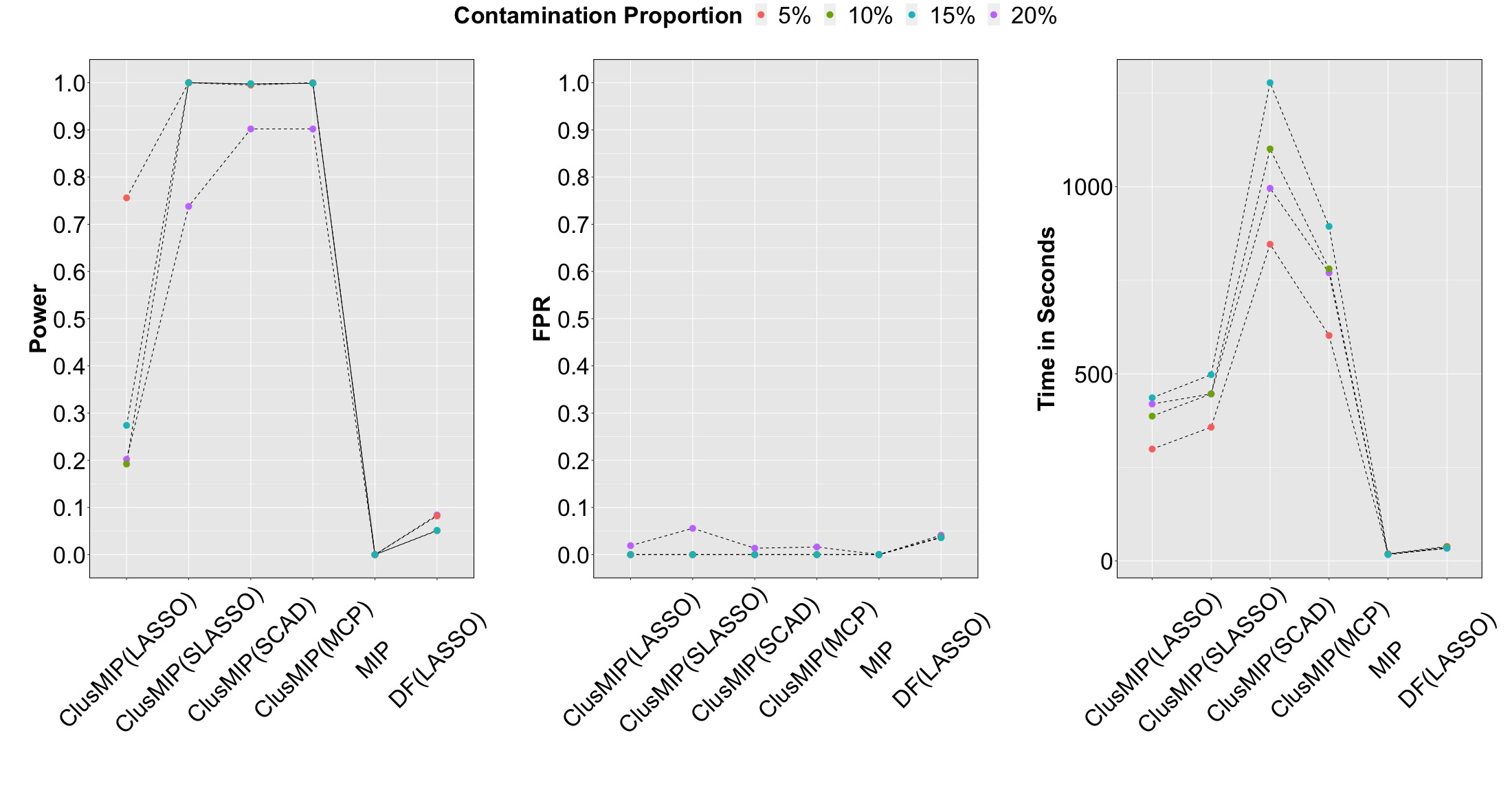
Figure 3: Assessment under the linear regression model, Perturbation Model II, $\kappa_{\text{Linear},\textbf{X}}$=5 and $\textbf{X}_{\text{Tp(0)}}$.

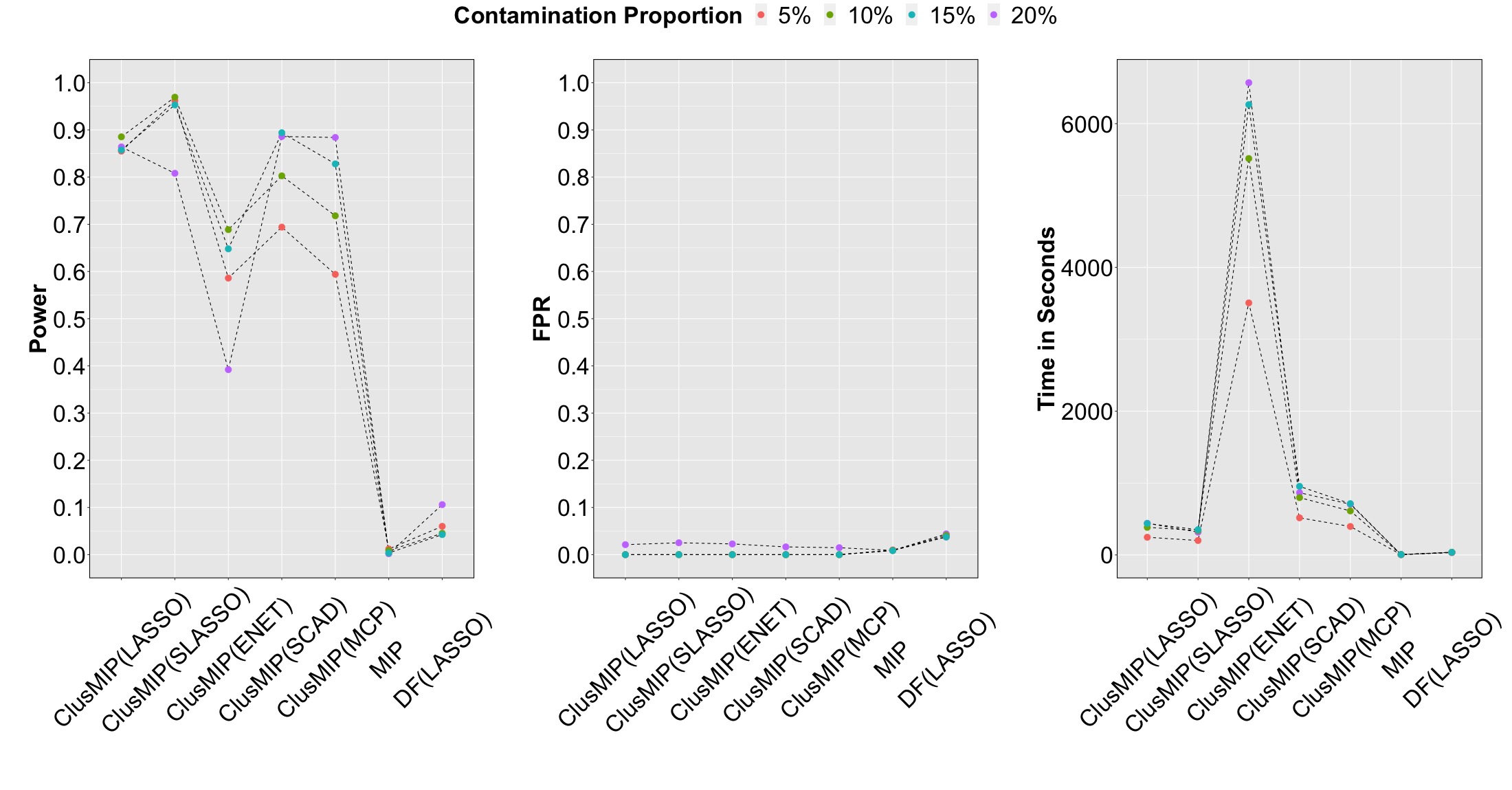
Figure 4: Assessment under the linear regression model, Perturbation Model II, $\kappa_{\text{Linear},\textbf{X}}$=5 and $\textbf{X}_{\text{Tp(0.5)}}$.

1. Power: under all types of design matrices, perturbation scales and contamination proportions, the detection powers of the two existing methods, MIP and DF(LASSO) are no more than 0.11, uniformly and considerably falling behind those of the ClusMIP procedure. This indicates that both approaches may not be able to accurately capture multiple influential points under this specific perturbation formulation. While the under-performance for the DF(LASSO) lies in its leave-one-out design, for MIP, we postulate that augmenting disturbance to the predictors while keeping the response vector intact is unlikely to impose sufficient impact on the marginal correlation-based HIM measure. Thus, true influential points are masked from being detected, leading to low detection power.

2. Power: when $\kappa_{\text{Linear},\textbf{X}}$=5 and $\textbf{X}=\textbf{X}_{\text{Tp(0)}}$, we observe that $\text{Power}_{\text{ClusMIP}(\text{SLASSO})}$,
   $\text{Power}_{\text{ClusMIP}(\text{SCAD})}$ and $\text{Power}_{\text{ClusMIP}(\text{MCP})}$ are almost uniformly 1.00 regardless of contamination proportion except for $\zeta$=5$\%$. In contrast, $\text{Power}_{\text{ClusMIP}(\text{LASSO})}$ is significantly lower, ranging between 0.20 and 0.76. When predictors are correlated, the patterns of detection power conspicuously deviate from those of the independent case. To be precise, only $\text{Power}_{\text{ClusMIP}(\text{SLASSO})}$ is able to achieve at least 0.95 (except for $\zeta$=5$\%$), followed by $\text{Power}_{\text{ClusMIP}(\text{LASSO})}$ ranging between 0.80 and 0.90. On the other hand, higher variation is seen in $\text{Power}_{\text{ClusMIP}(\text{SCAD})}$ and $\text{Power}_{\text{ClusMIP}(\text{MCP})}$, fluctuating between 0.60 and 0.90. Furthermore, $\text{Power}_{\text{ClusMIP}(\text{ENET})}$ is the lowest, varying between 0.40 and 0.70.

3. Power: when $\kappa_{\text{Linear},\textbf{X}}$ increases to 10 and for all types of design matrices, all the $\text{Power}_{\text{ClusMIP}(\text{LASSO})}$, $\text{Power}_{\text{ClusMIP}(\text{SLASSO})}$, $\text{Power}_{\text{ClusMIP}(\text{SCAD})}$ and $\text{Power}_{\text{ClusMIP}(\text{MCP})}$ approximately attain 1.00 except for $\text{Power}_{\text{ClusMIP}(\text{LASSO})}$ at $\zeta=15\%$ and $20\%$ for $\textbf{X}_{\text{Tp(0)}}$. In contrast, $\text{Power}_{\text{ClusMIP}(\text{ENET})}$ falls far behind, which is no more than 0.40.

4. FPR and Computation Time: the patterns for FPR and Computation Time are generally analogous to the corresponding ones identified for Perturbation Model I.

Linear Regression Model: Perturbation Model III

Under all the types of design matrices, perturbation scales and contamination proportions considered in our simulations, the generic relationships in detection power, FPR and computation time are similar to the ones identified under Perturbation Model I. In summary, only $\text{Power}_{\text{ClusMIP}(\text{SLASSO})}$ and $\text{Power}_{\text{MIP}}$ uniformly reach a level between 0.90 and 1.00, whereas $\text{Power}_{\text{DF}(\text{LASSO})}$ is consistently less than 0.10. In comparison, the detection powers of the ClusMIP for the remaining model selectors fluctuate in between 0.20 and 0.80. In addition, as the perturbation scale increases, we observe improved detection powers for all the procedures.

5 Analysis of Neurologic Signature of Physical Pain

In this section, based on the high-dimensional linear regression model (1), we analyze the performances of the aforementioned influential point detection procedures on the real dataset extracted from Lindquist et al. (2017) on pain level prediction via the fMRI data. Its background and characteristic is provided in Section 5.1. This is followed by presenting the assessment metrics, methods and implementation in Section 5.2. Analysis of results is provided in Section 5.3.

5.1 Background and Characteristic

This dataset sought to predict thermal-stimulated pain levels using multivariate patterns of brain activity and connectivity measured via fMRI data (Wager et al., 2013b; Lindquist et al., 2017). It consists of thirty-three healthy, right-handed participants with an overall average age of 27.9 years. Thermal stimulation was repeatedly delivered to the left volar forearm at six discrete temperatures: 44.3, 45.3, 46.3, 47.3, 48.3 and 49.3 $\tccentigrade$. After each stimulus, participants rated their pain on a 200-point scale. During the experiment, whole-brain fMRI data was acquired on an Achieva 3.0T TX MRI Scanner from Philips. Functional echo-planar imaging (EPI) images were acquired with: (i) repetition time (TR) = 2000 milliseconds (ms), (ii) time to echo (TE) = 20 ms, (iii) field of view (FOV) = 224 millimeters (mm), (iv) matrix = 64 $\times$ 64, (v) voxel size = 3.0 $\times$ 3.0 $\times$ 3.0 $\text{mm}^{3}$, and (vi) acquisition parameters are 42 interleaved slices for parallel imaging with sensitivity encoding (SENSE) factor 1.5. Structural images were acquired using high-resolution T1 spoiled gradient recall images (SPGR) for anatomical localization and warping to a standard space.

The structural T1-weighted images were co-registered to the mean functional image for each subject using the iterative mutual information-based algorithm implemented in the statistical parametric mapping (SPM) software package (Ashburner & Friston, 2005), and were then normalized to the Montreal Neurological Institute (MNI) space. In each functional dataset, initial volumes were removed to allow for stabilization of image intensity. Prior to processing functional images, we removed volumes with signal values that were outliers within the time series. This was done by first computing the mean and the standard deviation of intensity values across each slice, for each image, and then computing the Mahalanobis distances for the matrix of slice-wise mean and standard deviation values. Values with a significant $\chi^{2}$-value (corrected for multiple comparisons based on the more stringent of either false discovery rate or Bonferroni methods) were considered outliers. Next, functional images were slice-time corrected and motion-corrected using SPM. Functional images were warped to SPM’s normative atlas (warping parameters estimated from co-registered, high-resolution structural images) andinterpolated to 2 $\times$ 2 $\times$ 2 $\text{mm}^{3}$ voxels.

The processed data was then parcellated into 489 regions using the Clinical Affective Neuroimaging Laboratory (CANlab) combined whole-brain atlas. The dataset was further averaged across repeated trials at each of the six temperature levels, leading to a 198 by 489 matrix of brain activation. The pain ratings were similarly averaged over trials.

5.2 Assessment Metrics, Methods and Implementation

Three assessment metrics are included in our analysis, which are (i) $\widehat{\text{I}}^{\text{infl}}_{\text{Detection}(\text{Selector})}$, the estimated index set of influential points detected by the procedure “Detection” when a submodel is chosen by “Selector”, (ii) $\big{|}\widehat{\text{I}}^{\text{infl}}_{\text{Detection}(\text{Selector}})\big{\rvert}$, the cardinality of $\widehat{\text{I}}^{\text{infl}}_{\text{Detection}(\text{Selector})}$, and (iii) $\widehat{\text{T}}_{\text{Detection}(\text{Selector})}$, the time (seconds) required for obtaining $\widehat{\text{I}}^{\text{infl}}_{\text{Detection}(\text{Selector})}$.

To obtain the three assessment metrics, the two existing proposals, MIP and DF(LASSO), and the ClusMIP procedure with LASSO, SLASSO, ENET, SCAD and MCP as model selectors are included. Moreover, 10-fold CV is used to obtain tuning parameters for all the model selectors considered. In addition, all the computation is carried out on the computer with Intel(R) Core(TM) i7-6820(HQ) CPU $\MVAt$2.7Hz 2.7Hz and 32.0 GB of installed memory.

5.3 Analysis of Real Datasets

The assessment metrics of detection procedures are reported in Table 1, where we make the following observations and analyses:

1. Different combinations of influential observation detection and model selectors lead to drastically distinctive outcomes. Specifically, we can see that while no points are identified as influential by ClusMIP(SLASSO) and MIP, no less than 16 points are labelled influential by ClusMIP(LASSO), ClusMIP(ENET), ClusMIP(SCAD) and ClusMIP(MCP). This substantiates our previous explanation in Section 2 that the detection of influential observations in our context is intricately linked to the properties of variable selection procedures. To be more specific, different penalty functions ingrained in the model selectors reveal different sensitivities with respect to variable selection in the presence of potential influential observations. For this particular dataset, LASSO seems to be the most sensitive model selector, followed by SCAD and MCP. Furthermore, the matching performance of ClusMIP(SLASSO) and MIP aligns with our simulation results in Section 4.4, where $\text{Power}_{\text{ClusMIP}(\text{SLASSO})}$ and $\text{Power}_{\text{MIP}}$ are similar under certain scenarios.

   Table 1: Assessment Metrics for the Pain Prediction Dataset (Lindquist et al., 2017)

   Detection(Selectors)	$\widehat{\text{I}}^{\text{infl}}_{\text{Detection(Selector)}}$	$\big{|}\widehat{\text{I}}^{\text{infl}}_{\text{Detection (\text{Selector}})}\big{\rvert}$	$\widehat{\text{T}}_{\text{Detection(Selector)}}$
   ClusMIP(LASSO)	3, 7, 13, 14, 15, 19, 22, 25, 26, 43, 44, 49, 50, 52, 55, 56, 57, 58, 62, 67, 75, 79, 80, 81, 103, 115, 122, 123, 124, 127, 145, 147, 157, 158, 159, 164, 165, 169, 170, 172, 175, 176, 194	42	3214.03
   ClusMIP(SLASSO)	N.A.	0	2103.24
   ClusMIP(ENET)	31, 49, 50, 52, 55, 58, 76, 79, 115, 122, 124, 158, 169, 170, 172, 194	16	45944.46
   ClusMIP(SCAD)	31, 43, 49, 52, 55, 57, 62, 76, 80, 86, 103, 121, 133, 134, 145, 146, 157, 159, 164, 165, 173, 177, 181, 182, 193	25	6474.15
   ClusMIP(MCP)	13, 19, 26, 49, 52, 55, 57, 58, 73, 76, 86, 103, 121, 124, 134, 145, 147, 151, 163, 164, 165, 182	22	5059.49
   MIP	N.A.	0	5.27
   DF(LASSO)	2, 57, 84, 119, 153, 159, 168, 174, 198	9	64.83

2. For ClusMIP(LASSO) and ClusMIP(ENET), we can see that $\widehat{\text{I}}^{\text{infl}}_{\text{ClusMIP(ENET)}}$ is almost a proper subset of $\widehat{\text{I}}^{\text{infl}}_{\text{ClusMIP(LASSO)}}$, except for observations 31 and 76. Indeed, $\lvert\widehat{\text{I}}^{\text{infl}}_{\text{ClusMIP(LASSO)}}\rvert$ is the largest among all procedures considered. One possible explanation is that for this dataset, predictors which are multivariate brain activity patterns represented by voxels are expected to be highly correlated. As such, certain significant predictors may be de-selected by the LASSO. On the other hand, the unification of both $\ell_{1}$ and $\ell_{2}$ penalties embedded in the ENET facilitates the improved performance in variable selection. Thus, the submodel selected by LASSO may be more parsimonious than the one selected by ENET. This necessarily implies that in the finite sample, the submodel selected by ENET may demonstrate better goodness-of-fit than the one chosen by LASSO. Therefore, in the presence of influential observations, LASSO may have a higher tendency to be impacted by perturbation in variable selection than the ENET.

3. $\widehat{\text{I}}^{\text{infl}}_{\text{DF}(\text{LASSO})}$ hardly overlaps with those identified by other methods, except for the observations 57 and 169. This is mainly due to the embedded leave-one-out design, implying its inability to accurately capture multiple influential points.

   

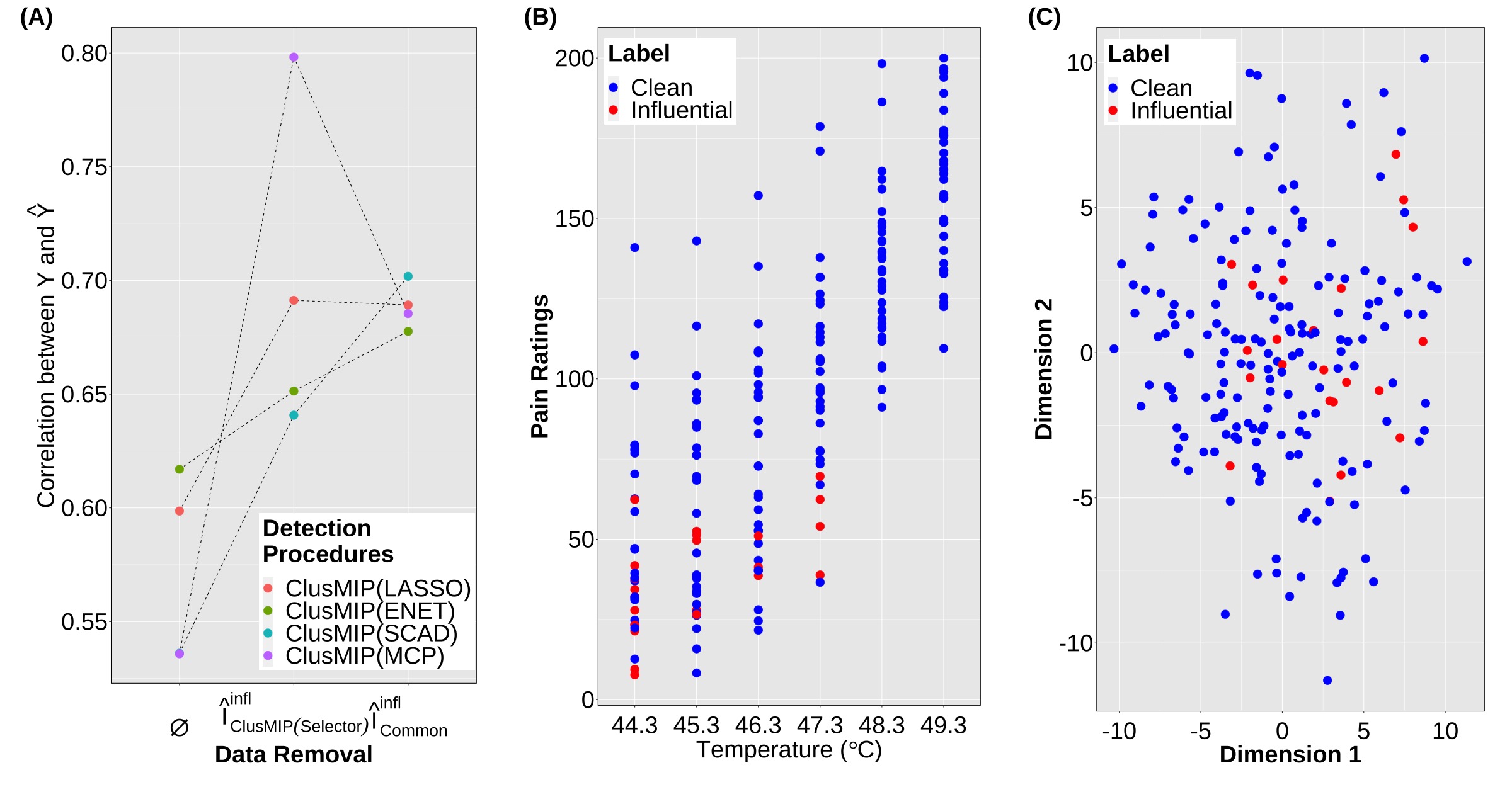
   Figure 5: (A): predictive power of the full and reduced datasets; (B): pain scores as a function of $\widehat{\text{I}}^{\text{infl}}_{\text{ClusMIP(MCP)}}$; (C): the first two dimensions from multi-dimensional scaling.

4. We have $\widehat{\text{I}}^{\text{infl}}_{\text{Common}}\coloneqq\ \widehat{\text{I}}^{\text{infl}}_{\text{ClusMIP}(\text{LASSO})}\ \cap\ \widehat{\text{I}}^{\text{infl}}_{\text{ClusMIP}(\text{ENET})}\ \cap\ \widehat{\text{I}}^{\text{infl}}_{\text{ClusMIP}(\text{SCAD})}\ \cap\ \widehat{\text{I}}^{\text{infl}}_{\text{ClusMIP}(\text{MCP})}=\{49,52,55\}$. As such, observations 49, 52 and 55 may serve as observations of interest that could undergo further studies. The first two observations correspond to two different temperatures measured on the same subject, indicating this may be a subject that needs to be further investigated. In addition, the first and third observation correspond to the lowest temperature, possibly indicating subjects that have a differing pain threshold than other subjects. Indeed, graphical illustration of pain ratings as a function of $\widehat{\text{I}}^{\text{infl}}_{\text{ClusMIP(Selector)}}$ (Figure 5(B)) indicates that the majority correspond to low pain ratings under each designated temperature, a pattern which holds over all the model selectors. In fact, the low pain score primarily contributes to the “outlyingness” of the identified influential points, since no anomalies in the feature space are detected as seen in the multi-dimensional scaling plot (Figure 5(C)). This may be explained by the fact that this temperature is generally considered warm, but not painful, thus differentiating it from other temperature levels.

5. Different model selection outcomes are observed when a submodel is selected from the full dataset and the one after removing $\widehat{\text{I}}^{\text{infl}}_{\text{ClusMIP(Selector)}}$. In Figure 6, we highlight the brain regions selected via MCP with color intensities represented by the corresponding coefficient estimates obtained from the full and reduced datasets. Panels A and B demonstrate such discrepancy in selected regions, while Panels C, D and E pinpoint common and uniquely selected regions from the two datasets. Six regions are common to both models, including primary visual, frontoparietal, dorsal attention, and default mode areas, as well as the amygdala. Regions unique to the full model include the cerebellum, while regions unique to the reduced model include ventral attention and additional frontoparietal areas.

   

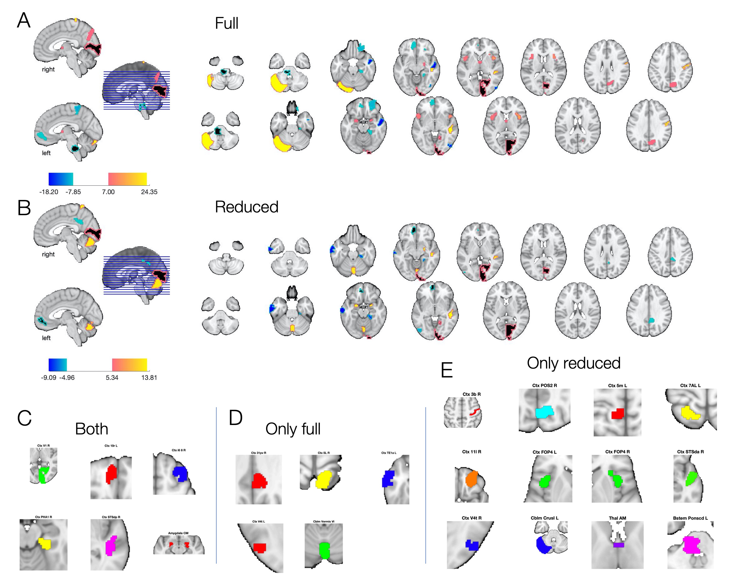
   Figure 6: (A) and (B): brain regions selected by MCP from the full and reduced datasets with color intensities denoting the scales of coefficient estimates; (C): common regions selected from both datasets; (D) and (E): unique regions selected respectively from the full and reduced dataset.

6. In Figure 5 (A), we observe improved sample correlation between the real and predicted pain scores after removing $\widehat{\text{I}}^{\text{infl}}_{\text{ClusMIP(Selector)}}$ and $\widehat{\text{I}}^{\text{infl}}_{\text{Common}}$ for all the model selectors. For example, such correlation increases from 0.53 to 0.80 after removing $\widehat{\text{I}}^{\text{infl}}_{\text{MCP}}$, illustrating the advantage for identifying and removing influential points.

6 Conclusion

In this manuscript, we highlight the important issue of identifying observations that could unduly affect the choice of a stochastically selected submodel, which is largely ignored in the existing influential diagnosis literature. Indeed, inappropriate handling of such observations unavoidably leads to an inaccurate selected submodel (Figure 1 in Section 1 of the Supplementary Materials), giving rise to detrimental effects on the validity and reproducibility in downstream statistical inference. To capture them, especially under the high-dimensional setting, we have proposed the so-called ClusMIP detection procedure, and evaluated it alongside two existing proposals, the DF(LASSO) and MIP. From the simulation results in Section 4, we see that the DF(LASSO) is unable to detect multiple influential points due to its leave-one-out design. On the other hand, the MIP is a computationally efficient and effective diagnostic metric in dealing with contamination introduced only on the response, and on the response and predictors simultaneously. Yet, it under-performs when contamination is solely included in the predictors. In comparison, the performance of the ClusMIP varies according to data generating mechanisms and model selectors. In fact, the variation in the performance of ClusMIP as a function of model selector provides insights on the sensitivities of different model selectors, which is one essential objective of this manuscript. To be more precise, under the linear regression model and when predictors are independent, ClusMIP(SLASSO) offers relatively satisfactory solutions in detecting all the influential points, implying that both model selectors are sensitive to their presence. In contrast, other model selectors may not be sensitive as shown in their detection powers. Yet, one limitation of the ClusMIP procedure lies in its computational cost, which depends on the outcome of the selected high-dimensional clustering procedure.

In addition to the above conclusions, we now outline possible extensions of the current work. First, we recognize significant variation in the detection performances of the ClusMIP algorithm on different model selectors. Initial investigation reveals that in the second stage of the procedure, the GDF measure (5) associated with some selectors may not be sufficiently large to recognize true influential points. Yet, the underlying theoretical logic, which is intricately linked to the breakdown points for model selectors that are briefly discussed in Section 2, is unclear and currently undergoing further investigation. Second, the exact finite- and large-sample distributional properties of $\tau_{i}$ in (5) have not been studied, which may pave the way for alternative parametric and re-sampling approximation.

Dongliang Zhang is supported in part by NIH grant R01MH129397 from the National Institute of Mental Health (NIMH). Masoud Asgharian is supported by the Natural Science and Engineering Research Council of Canada (NSERC RGPIN-2018-05618). Martin A. Lindquist is supported in part by NIH grant R01 EB026549 from the National Institute of Biomedical Imaging and Bioengineering (NIBIB), and R01MH129397 from NIMH.

The Supplementary Materials referenced in Sections 1 to 5 contains data generating details of the motivating example, proofs of Theorems 1 to 3 and Corollary 1, algorithmic details of the RGD, MIP and RGDF procedures, comparison of different clustering procedures, and additional simulation details and plots.

References

- (1)
- Aldous (1977) Aldous, D. J. (1977), ‘Limit theorems for subsequences of arbitrarily-dependent sequences of random variables’, Z. Wahrsch. Verw. Gebiete pp. 1432–2064.
- Arthur & Vassilvitskii (2007) Arthur, D. & Vassilvitskii, S. (2007), K-means++: The advantages of careful seeding, in ‘Proceedings of the Eighteenth Annual ACM-SIAM Symposium on Discrete Algorithms’, p. 1027–1035.
- Ashburner & Friston (2005) Ashburner, J. & Friston, K. J. (2005), ‘Unified segmentation’, NeuroImage 26(3), 839–851.
- Belsley et al. (1980) Belsley, D., Kuh, E. & Welsch, R. E. (1980), Regression Diagnostics: Identifying Influential Data and Sources of Collinearity, John Wiley & Sons, Inc.
- Benjamini & Hochberg (1995) Benjamini, Y. & Hochberg, Y. (1995), ‘Controlling the false discovery rate: A practical and powerful approach to multiple testing’, J. R. Stat. Soc. Ser. B. Stat. Methodol. 57(1), 289–300.
- Beyer et al. (1999) Beyer, K., Goldstein, J., Ramakrishnan, R. & Shaft, U. (1999), When is “nearest neighbor” meaningful?, in ‘Database Theory — ICDT 1999’, pp. 217–235.
- Commenges (2003) Commenges, D. (2003), ‘Transformations which preserve exchangeability and application to permutation tests’, J. Nonparametr. Stat. 15(2), 171–185.
- Cook (1977) Cook, R. D. (1977), ‘Detection of influential observation in linear regression’, Technometrics 19(1), 15–18.
- de Finetti (1931) de Finetti, B. (1931), ‘Funzione caratteristica di un fenomeno aleatorio’, Atti R. Accad. Naz. Lincei, Ser. 6. Memorie, Cl. Sci. Fis., Mat. Natur. 4 pp. 251–299.
- Donoho (1982) Donoho, D. L. (1982), ‘Breakdown properties of multivariate location estimators’, Ph. D. qualifying paper, Dept. Statistics, Harvard University .
- Fan et al. (2014) Fan, J., F. Han, F. & Liu, H. (2014), ‘Challenges of big data analysis’, Natl. Sci. Rev. 1(2), 293–314.
- Fan & Li (2001) Fan, J. & Li, R. (2001), ‘Variable selection via nonconcave penalized likelihood and its oracle properties’, J. Amer. Statist. Assoc. 96(456), 1348–1360.
- Fan & Lv (2010) Fan, J. & Lv, J. (2010), ‘A selective overview of variable selection in high dimensional feature space’, Statist. Sinica 20(1), 101–148.
- Freedman (1983) Freedman, D. A. (1983), ‘A note on screening regression equations’, Amer. Statist. 37(2), 152–155.
- Galambos (1973) Galambos, J. (1973), ‘A general Poisson limit theorem of probability theory’, Duke Math. J. 40(3), 581–586.
- Hadi & Simonoff (1993) Hadi, A. S. & Simonoff, J. S. (1993), ‘Procedures for the identification of multiple outliers in linear models’, J. Amer. Statist. Assoc. 88(424), 1264–1272.
- Hahn & Zhang (1998) Hahn, M. G. & Zhang, G. (1998), Distinctions between the regular and empirical central limit theorems for exchangeable random variables, in ‘High Dimensional Probability’, pp. 111–143.
- Hall et al. (2005) Hall, P., Marron, J. S. & Neeman, A. (2005), ‘Geometric representation of high dimension, low sample size data’, J. R. Stat. Soc. Ser. B. Stat. Methodol. 67(3), 427–444.
- Hampel (1971) Hampel, F. R. (1971), ‘A general qualitative definition of robustness’, Ann. Math. Statist. 42(6), 1887–1896.
- Hampel et al. (1986) Hampel, F. R., Ronchetti, E. M., Rousseeuw, P. J. & Stahel, W. A. (1986), Robust Statistics: The Approach Based on Influence Functions, Wiley.
- Haynes (2015) Haynes, J.-D. (2015), ‘A primer on pattern-based approaches to fmri: principles, pitfalls, and perspectives’, Neuron 87(2), 257–270.
- Hinton & Roweis (2002) Hinton, G. E. & Roweis, S. (2002), Stochastic neighbor embedding, in ‘Advances in Neural Information Processing Systems’, Vol. 15.
- Klass & Teicher (1987) Klass, M. & Teicher, H. (1987), ‘The Central Limit Theorem for Exchangeable Random Variables Without Moments’, Ann. Probab. 15(1), 138–153.
- Leger & Altman (1993) Leger, C. & Altman, N. (1993), ‘Assessing influence in variable selection problems’, J. Amer. Statist. Assoc. 88(422), 547–556.
- Lindquist et al. (2017) Lindquist, M. A., .Krishnan, A., López-Solà, M., Jepma, M., Woo, C.-W., Koban, L., Roy, M., Atlas, L. Y., Schmidt, L., Chang, L. J., Losin, E. A. R., Eisenbarth, H., Ashar, Y. K., Delk, E. & Wager, T. D. (2017), ‘Group-regularized individual prediction: theory and application to pain’, NeuroImage 145, 274–287.
- Lindquist et al. (2008) Lindquist, M. A. et al. (2008), ‘The statistical analysis of fmri data’, Statistical science 23(4), 439–464.
- Ng et al. (2001) Ng, A., Jordan, M. & Weiss, Y. (2001), On spectral clustering: Analysis and an algorithm, in ‘Advances in Neural Information Processing Systems’, Vol. 14.
- Ombao et al. (2016) Ombao, H., Lindquist, M., Thompson, W. & Aston, J. (2016), Handbook of Neuroimaging Data Analysis, CRC Press.
- Orru et al. (2012) Orru, G., Pettersson-Yeo, W., Marquand, A. F., Sartori, G. & Mechelli, A. (2012), ‘Using support vector machine to identify imaging biomarkers of neurological and psychiatric disease: a critical review’, Neuroscience & Biobehavioral Reviews 36(4), 1140–1152.
- Pollard (1981) Pollard, D. (1981), ‘Strong consistency of -means clustering’, Ann. Statist. 9(1), 135–140.
- Rajaratnam et al. (2019) Rajaratnam, B., Roberts, S., Sparks, D. & Yu, H. (2019), ‘Influence diagnostics for high-dimensional lasso regression’, J. Comput. Graph. Statist. 28(4), 877–890.
- Sun & Zhang (2012) Sun, T. & Zhang, C.-H. (2012), ‘Scaled sparse linear regression’, Biometrika 99(4), 879–898.
- Sun et al. (2012) Sun, W., Wang, J. & Fang, Y. (2012), ‘Regularized k-means clustering of high-dimensional data and its asymptotic consistency’, Electronic Journal of Statistics 6, 148 – 167.
- Tibshirani (1996) Tibshirani, R. (1996), ‘Regression shrinkage and selection with the lasso’, J. R. Stat. Soc. Ser. B. Stat. Methodol. 58, 267–288.
- Wager et al. (2013a) Wager, T. D., Atlas, L. Y., Lindquist, M. A., Roy, M., Woo, C.-W. & Kross, E. (2013a), ‘An fmri-based neurologic signature of physical pain’, New England Journal of Medicine 368(15), 1388–1397.
- Wager et al. (2013b) Wager, T. D., Atlas, L. Y., Lindquist, M., Roy, M., Woo, C.-W. & Kross, E. (2013b), ‘An fMRI-based neurologic signature of physical pain’, N. Engl. J. Med. 368(15), 1388–1397.
- Wang et al. (2022) Wang, G., Datta, A. & Lindquist, M. A. (2022), ‘Bayesian functional registration of fmri activation maps’, The Annals of Applied Statistics 16(3), 1676–1699.
- Zhang (2010) Zhang, C.-H. (2010), ‘Nearly unbiased variable selection under minimax concave penalty’, Ann. Statist. 38(2), 894–942.
- Zhao et al. (2013) Zhao, J., Leng, C., Li, L. & Wang, H. (2013), ‘High-dimensional influence measure’, Ann. Statist. 41(5), 2639–2667.
- Zhao et al. (2019) Zhao, J., Liu, C., Niu, L. & Leng, C. (2019), ‘Multiple influential point detection in high dimensional regression spaces’, J. R. Stat. Soc. Ser. B. Stat. Methodol. 81(2), 385–408.
- Zhao et al. (2015) Zhao, J., Zhang, Y. & Niu, L. (2015), Detecting multiple influential observations in high dimensional linear regression, in ‘Advanced Intelligent Computing Theories and Applications’, Springer International Publishing, pp. 55–64.
- Zhao & Yu (2006) Zhao, P. & Yu, B. (2006), ‘On model selection consistency of lasso’, J. Mach. Learn. Res. 7, 2541–2563.
- Zou & Hastie (2005) Zou, H. & Hastie, T. (2005), ‘Regularization and variable selection via the elastic net’, J. R. Stat. Soc. Ser. B. Stat. Methodol. 67(2), 301–320.