Realized Stochastic Volatility Model with Skew-t Distributions for Improved Volatility and Quantile Forecasting

Abstract

Forecasting volatility and quantiles of financial returns is essential for accurately measuring financial tail risks, such as value-at-risk and expected shortfall. The critical elements in these forecasts involve understanding the distribution of financial returns and accurately estimating volatility. This paper introduces an advancement to the traditional stochastic volatility model, termed the realized stochastic volatility model, which integrates realized volatility as a precise estimator of volatility. To capture the well-known characteristics of return distribution, namely skewness and heavy tails, we incorporate three types of skew-$t$ distributions. Among these, two distributions include the skew-normal feature, offering enhanced flexibility in modeling the return distribution. We employ a Bayesian estimation approach using the Markov chain Monte Carlo method and apply it to major stock indices. Our empirical analysis, utilizing data from US and Japanese stock indices, indicates that the inclusion of both skewness and heavy tails in daily returns significantly improves the accuracy of volatility and quantile forecasts.

Keywords: Bayesian estimation, Markov chain Monte Carlo, Realized volatility, Skew-t distribution, Stochastic volatility

1 Introduction

Financial volatility, defined as the standard deviation or variance of asset returns, exhibits stochastic variation over time, making its accurate forecasting crucial for financial risk management. Historically, time-varying volatility estimation and forecasting relied on two classes of time-series models using financial returns: the generalized autoregressive conditional heteroskedasticity (GARCH) methodologies, as per Engle (1982) and Bollerslev (1986), and the stochastic volatility (SV) model, introduced by Taylor (1994). These models, known for capturing volatility clustering and high volatility persistence, have evolved to accommodate volatility asymmetry or the leverage effect – the observed negative correlation between today’s return and tomorrow’s volatility in stock markets. One notable development is the exponential GARCH (EGARCH) model by Nelson (1991).

In more recent years, realized volatility (RV) has emerged as a predominant method for volatility estimation, replacing traditional models. RV, computed daily as the sum of squared intraday returns, is thoroughly reviewed by Andersen and Benzoni (2009) and McAleer and Medeiros (2008). To model RV dynamics, various studies, such as Andersen et al. (2003), have shown that daily RV may follow a long-memory process, leading to the use of autoregressive fractionally integrated moving average (ARFIMA) models (refer to Beran (1994) for a detailed discussion on long-memory and ARFIMA models). Additionally, the heterogeneous autoregressive (HAR) model, proposed by Corsi (2009), is widely used for modeling the dynamics of RV. Although not a long-memory model per se, the HAR model effectively approximates long-memory processes.

Despite the improved volatility forecasts offered by ARFIMA and HAR models over GARCH and SV models, RV is susceptible to biases from market microstructure noise and non-trading hours. Techniques such as the multiscale estimators by Zhang et al. (2005) and Zhang (2006a), the pre-averaging approach by Jacod et al. (2009), and the realized kernel (RK) method by Barndorff-Nielsen et al. (2008, 2009) have been developed to mitigate these biases. For further details, see Aït-sahalia and Mykland (2009), Ubukata and Watanabe (2014), and Liu et al. (2015).

Addressing the bias in RV, two hybrid model classes have been introduced: the realized stochastic volatility (RSV) model, as proposed by Takahashi et al. (2009), Dobrev and Szerszen (2010), and Koopman and Scharth (2013), and the realized GARCH (RGARCH) and realized EGARCH (REGARCH) models, introduced by Hansen et al. (2012) and Hansen and Huang (2016), respectively. Although previous studies have compared the volatility forecasting abilities of these models within their respective classes, a comprehensive cross-class comparison has been limited. Notable exceptions are Takahashi et al. (2021) and Takahashi et al. (2023), which evaluate the forecasting abilities of various models, including SV, EGARCH, RSV, and REGARCH models.

In addition to volatility forecasting, accurately predicting financial tail risks, such as value-at-risk (VaR) and expected shortfall (ES), is essential. Financial return distributions often exhibit heavier tails and more peakedness than the normal distribution, a phenomenon known as leptokurtosis. While time-varying volatility partly explains this heavy-tailed nature, the conditional return distribution on volatility may still exhibit leptokurtic characteristics and skewness. Consequently, various skew Student’s $t$ distributions have been incorporated into volatility models (Abanto-Valle et al., 2015; Kobayashi, 2016). Notably, the generalized hyperbolic (GH) skew Student’s $t$ distribution, as discussed in Aas and Haff (2006), has been applied to both SV (Nakajima and Omori, 2012; Leão et al., 2017) and RSV models (Trojan, 2013; Nugroho and Morimoto, 2014, 2016; Takahashi et al., 2016).

Building on this framework, the RSV model is extended to include three types of skew-$t$ distributions, and a Bayesian estimation scheme using a Markov chain Monte Carlo (MCMC) method is developed. These skew-$t$ distributions are those proposed by Azzalini (1985) and Fernández and Steel (1995), along with the GH skew-$t$ distribution. In our empirical analysis using the Dow Jones Industrial Average (DJIA) and the Nikkei 225 (N225) data, we evaluate the volatility, VaR, and ES forecasts of RSV models as well as SV, EGARCH, and REGARCH models. Forecasts are assessed using mean squared error and quasi likelihood loss functions for volatility, and the joint loss function proposed by Fissler and Ziegel (2016), with specifications suggested by Patton et al. (2019), for VaR and ES. Implementing the predictive ability test by Giacomini and White (2006) and the model confidence set by Hansen et al. (2011), our results indicate that RV significantly improves forecasting performance. The RSV models, especially those incorporating skew-$t$ distributions, demonstrate superior performance, corroborating and extending findings from previous studies.

The remainder of the paper is structured as follows. Section 2 introduces the basic SV model and the RSV models, which incorporate skew-$t$ distributions, along with a brief overview of RV. Section 3 delves into the Bayesian estimation methodology, utilizing MCMC simulations, and discusses various measures for evaluating forecast performance. Section 4 presents an empirical study employing financial stock indices data. Finally, Section 5 provides a conclusion, summarizing key findings and implications of the study.

2 Model

2.1 Stochastic Volatility Model

First, let’s define the daily return of an asset as

$$y_{t}=\log p_{t}-\log p_{t-1},$$

where $p_{t}$ represents the closing price on day $t$. We further define the volatility as a variance of $y_{t}$ as

$$\text{E}[y_{t}^{2}]=\sigma_{t}^{2}=\exp(h_{t}).$$

The term $h_{t}$ denotes the logarithm of volatility. This logarithmic volatility, $h_{t}$, is considered a latent variable. It is presumed to follow a stationary first-order autoregressive (AR(1)) process characterized by the autoregressive parameter $\phi$ and a mean of $\mu$. Additionally, the absolute value of $\phi$ should be less than one to ensure stationarity. With $h_{t}$ given at time $t$, the SV model can be detailed as:

$$y_{t} =\epsilon_{t}\exp\left(\frac{h_{t}}{2}\right),\quad t=1,\ldots,n,$$ (1)

$$h_{t+1} =\mu+\phi(h_{t}-\mu)+\eta_{t},\quad t=1,\ldots,n-1,\quad|\phi|<1,$$ (2)

$$h_{1} \sim N\left(\mu,\frac{\sigma_{\eta}^{2}}{1-\phi^{2}}\right),$$ (3)

$$\epsilon_{t} \sim N(0,1),$$ (4)

$$\eta_{t}|\epsilon_{t} \sim N(\rho\sigma_{\eta}\epsilon_{t},(1-\rho^{2})\sigma_{\eta}^{2}).$$ (5)

Here, we assume a stationary distribution for the initial log latent volatility, $h_{1}$. The AR(1) process for $h_{t}$ is intended to describe volatility clustering. This is the phenomenon where significant price fluctuations tend to occur in close succession. The disturbance vector $(\epsilon_{t},\eta_{t})^{\prime}$ is believed to obey a bivariate normal distribution with a correlation $\rho$ between $\epsilon_{t}$ and $\eta_{t}$ (or equivalently, between $y_{t}$ and $h_{t+1}$). A negative correlation, where $\rho<0$, indicates an asymmetry or a leverage effect. This suggests that a decline in $y_{t}$ is often followed by an increase in $h_{t+1}$.

2.2 Realized Volatility

In the SV model, the volatility $\exp(h_{t})$ is considered a latent variable since $h_{t}$ is unobserved. Recently, due to the availability of high-frequency data, RV has been proposed as an estimator for true volatility using intraday data. We first define the true volatility at time $t$. Let $p(s)$ denote the logarithm of the price of the asset at time $s$, and assume it follows the continuous time diffusion process given by

$$dp(s)=\mu(s)ds+\sigma(s)dW(s),$$ (6)

where $\mu(s)$, $\sigma^{2}(s)$, and $W(s)$ represent the drift, the volatility, and the Wiener process, respectively. The true volatility for day $t$ is defined as

$$IV_{t}=\int_{t}^{t+1}\sigma^{2}(s)ds,$$ (7)

which is also referred to as the integrated volatility. Suppose we have $n$ intraday observations for day $t$, given by $\left\{r_{t},r_{t+1/n},\ldots,r_{t+(n-1)/n}\right\}$. Then the RV, as an estimator of $IV_{t}$, is defined by

$$RV_{t}=\sum_{i=0}^{n-1}r_{t+i/n}^{2}.$$ (8)

Under certain conditions, it can be shown that $RV_{t}$ converges to $IV_{t}$ as $n\rightarrow\infty$. However, these conditions are often not satisfied in practice with high-frequency data, resulting in a bias in the estimator.

One source of this bias arises from non-trading hours during which we lack intraday observations. If we ignore the non-trading hours to compute the RV, we underestimate the true volatility for a whole day (24 hours). To address the non-trading hours, Hansen and Lunde (2005) proposed adjusting $RV_{t}$ as follows:

$$RV_{t}^{HL}=c_{HL}RV_{t},\quad c_{HL}=\frac{\sum_{t=1}^{n}(y_{t}-\overline{y})^{2}}{\sum_{t=1}^{n}RV_{t}}\quad\text{and}\quad\overline{y}=\frac{1}{n}\sum_{t=1}^{n}y_{t},$$ (9)

where $RV_{t}$ represents the RV when non-trading hours are ignored. The average of $RV_{t}^{HL}$ is set equal to the sample variance of the daily returns.

Another source of bias is the microstructure noise. The actual asset prices are observed with microstructure noise, which results in autocorrelations in the asset returns and violates these assumptions. The effect of microstructure noise is known to become larger as the time interval between observed prices becomes smaller. The optimal time intervals to compute the RV have been investigated in the literature (Aït-Sahalia et al., 2005; Bandi and Russell, 2006, 2008; Liu et al., 2015). Alternative estimators, such as the two or multi-scale estimator (Zhang et al., 2005; Zhang, 2006b) and the preaveraging estimator (Jacod et al., 2009), have also been proposed. In the empirical study in Section 4, we use the RK (Barndorff-Nielsen et al., 2008) as an unbiased volatility estimator. The RK for day $t$ is defined as

$$RK_{t}=\sum_{h=-H}^{H}k\left(\frac{h}{H+1}\right)\gamma_{h},$$ (10)

where $H$ is the bandwidth, $k(\cdot)\in[0,1]$ is a non-stochastic weight function, and

$$\gamma_{h}=\sum_{i=|h|+1}^{m}r_{t-1+i/m}r_{t-1+(i-|h|)/m}.$$ (11)

For the choice of $k(\cdot)$, Barndorff-Nielsen et al. (2009) have suggested the Parzen kernel function and provided a detailed procedure for the choice of $H$.

Alternatively, these biases can be incorporated into two classes of hybrid models: the RSV and RGARCH models. In particular, the RSV model proposed by Takahashi et al. (2009) adjusts the bias of the RV by estimating the model parameter as discussed in Section 2.3.

2.3 Realized Stochastic Volatility Model

Takahashi et al. (2009) introduced an additional source of information regarding the true volatility. Besides the measurement equation for the daily return $y_{t}$, they also considered that of the log RV, $x_{t}=\log RV_{t}$. Let $h_{t}$ denote the logarithm of the true volatility, $h_{t}=\log IV_{t}$. The RSV model is defined as follows:

$$x_{t} =\xi+h_{t}+u_{t},\quad t=1,\ldots,n,$$ (12)

$$y_{t} =\epsilon_{t}\exp\left(\frac{h_{t}}{2}\right),\quad t=1,\ldots,n,$$ (13)

$$h_{t+1} =\mu+\phi(h_{t}-\mu)+\eta_{t},\quad t=1,\ldots,n-1,\quad|\phi|<1,$$ (14)

$$h_{1} \sim N\left(\mu,\frac{\sigma_{\eta}^{2}}{1-\phi^{2}}\right),$$ (15)

$$u_{t} \sim N(0,\sigma_{u}^{2}),$$ (16)

$$\epsilon_{t} \sim N(0,1),$$ (17)

$$\eta_{t}|\epsilon_{t} \sim N(\rho\sigma_{\eta}\epsilon_{t},(1-\rho^{2})\sigma_{\eta}^{2}),$$ (18)

where $u_{t}$ is assumed to be independent of $(\epsilon_{t},\eta_{t})$ for simplicity. In general, equation (12) could be replaced by

$$x_{t}=\xi+\psi h_{t}+u_{t}.$$

However, empirical studies have found that this extension does not improve the forecasting performance of the volatilities, leading to the assumption $\psi=1$ as in Takahashi et al. (2009).

The parameter $\xi$ serves as a bias correction factor in $\log RV_{t}$, where $\xi=0$ implies that there is no bias. Ignoring the non-trading hours while computing the RV leads to an underestimation of $IV_{t}$, expecting a negative bias. Hansen and Lunde (2006) demonstrated that microstructure noise may induce either a positive or negative bias. Therefore, $\xi>0$ if the positive bias caused by microstructure noise dominates the negative bias from ignoring non-trading hours, and $\xi<0$ otherwise.

The distribution of $\epsilon_{t}$ corresponds to the return distribution conditional on the effect of the time-varying volatility. Although the inclusion of stochastic volatility $h_{t}$ captures the heavy tails of financial returns, the distribution of $\epsilon_{t}$ can be further assumed to have heavy tails, such as a Student’s $t$ distribution. Moreover, financial returns may also exhibit skewness. The excess kurtosis and negative skewness can be accounted for by adopting an asymmetric heavy-tailed distribution for daily returns.

For the SV model, Nakajima and Omori (2012) and Leão et al. (2017) adapted the GH skew Student’s $t$ distribution proposed by Aas and Haff (2006). Additionally, Abanto-Valle et al. (2015) employed the skew Student’s $t$ distribution proposed by Azzalini and Capitanio (2003), while Kobayashi (2016) utilized the skew exponential power distribution. Furthermore, Steel (1998) extended the SV model using the method proposed by Fernández and Steel (1995). For the RSV model, Trojan (2013), Nugroho and Morimoto (2014, 2016), and Takahashi et al. (2016) adapted the GH skew Student’s $t$ distribution. In the following, we extend the RSV model in equations (12)–(18), henceforth referred to as the RSV-N model, by employing such distributions for $\epsilon_{t}$.

2.4 RSV Model with Student’s $t$ Distribution

The RSV model, when augmented with the Student’s $t$ distribution, will henceforth be referred to as the RSV-T model. This model is derived by modifying the distributions of $\epsilon_{t}$ and $\eta_{t}$ as described in equations (17)–(18), to:

$$\epsilon_{t} =z_{t}\sqrt{\frac{\lambda_{t}}{\mu_{\lambda}}},$$ (19)

$$z_{t} \sim N(0,1),$$ (20)

$$\eta_{t}|z_{t} \sim N(\rho\sigma_{\eta}z_{t},(1-\rho^{2})\sigma_{\eta}^{2}),$$ (21)

where

$$\lambda_{t} \stackrel{{\scriptstyle i.i.d.}}{{\sim}}IG\left(\frac{\nu}{2},\frac{\nu}{2}\right),\quad\mu_{\lambda}=E[\lambda_{t}]=\frac{\nu}{\nu-2},\quad\nu>2.$$ (22)

The parameter $\nu$ is the degrees of freedom, which governs the excess kurtosis not captured by the stochastic volatility $h_{t}$. As $\nu$ approaches infinity, the model reverts to the RSV-N model described in equations (12)–(18). It’s worth noting that the correlation between $\epsilon_{t}$ and $\eta_{t}$ now becomes a function of both $\rho$ and $\nu$, expressed as:

$$\text{Corr}[\epsilon_{t},\eta_{t}]=\frac{E\left[\sqrt{\lambda_{t}}\right]}{\sqrt{\mu_{\lambda}}}\rho,$$ (23)

where

$$E\left[\sqrt{\lambda_{t}}\right]=\sqrt{\frac{\nu}{2}}\frac{\Gamma\left(\frac{\nu-m}{2}\right)}{\Gamma\left(\frac{\nu}{2}\right)}.$$ (24)

2.5 RSV Model with GH Skew-$t$ Distribution

Takahashi et al. (2016) extend the RSV-N model delineated in (12)–(18) by incorporating the GH skew-$t$ distribution, hereafter referred to as the RSV-GH-ST model. This model is attained by substituting $\epsilon_{t}$ and $\eta_{t}$ in (17)–(18) with the ensuing mixture representation:

$$\epsilon_{t} =\frac{\beta(\lambda_{t}-\mu_{\lambda})+\sqrt{\lambda_{t}}z_{t}}{\sqrt{\beta^{2}\sigma_{\lambda}^{2}+\mu_{\lambda}}},$$ (25)

$$z_{t} \sim N(0,1),$$ (26)

$$\eta_{t}|z_{t} \sim N(\rho\sigma_{\eta}z_{t},(1-\rho^{2})\sigma_{\eta}^{2}),$$ (27)

where $\lambda_{t}$ and $\mu_{\lambda}$ are defined as in (22), and

$$\sigma_{\lambda}^{2}=V[\lambda_{t}]=E\left[\lambda_{t}^{2}\right]-\{E[\lambda_{t}]\}^{2}=\frac{2\nu^{2}}{(\nu-2)^{2}(\nu-4)},\quad\nu>4.$$ (28)

The term $\sqrt{\beta^{2}\sigma_{\lambda}^{2}+\mu_{\lambda}}$ standardizes the return ensuring that the variance of the return remains $\exp(h_{t})$. It is noteworthy that the correlation between $\epsilon_{t}$ and $\eta_{t}$ is now a function of $\rho$, $\nu$, and $\beta$, expressed by:

$$\text{Corr}[\epsilon_{t},\eta_{t}]=\frac{E\left[\sqrt{\lambda_{t}}\right]}{\sqrt{\beta^{2}\sigma_{\lambda}^{2}+\mu_{\lambda}}}\rho,$$ (29)

where $E\left[\sqrt{\lambda_{t}}\right]$ is specified in (24). When $\beta=0$, this model reverts to the RSV-T model.

The skewness and tail thickness of $\epsilon_{t}$ are concurrently determined by the parameter values of $\beta$ and $\nu$. To exhibit how the distribution shape varies with the values, we render the simulated density function of $\epsilon_{t}$ in Figure 1. We discern from (i) of the figure that a lower value of $\beta$ yields a more negative or left-skewed distribution with heavier tails. As stipulated, $\beta=0$ corresponds to a symmetric Student’s $t$ density. Conversely, from (ii), the density appears less skewed and has lighter tails as $\nu$ increases. Additionally, as $\nu\to\infty$ or $\lambda_{t}=1$ for all $t$, the distribution morphs into a normal distribution regardless of the value of $\beta$. Therefore, $\nu$ and $\beta$ can be interpreted as parameters regarding the tail thickness and skewness, respectively, albeit the overall shape of the distribution is determined by their joint values.

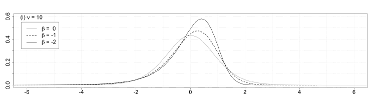
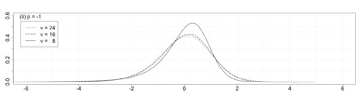
Figure 1: Simulated density function of the standardized GH skew-$t$ distribution in (25). (i) $\beta=0,-1,-2$ with $\nu=10$ fixed. (ii) $\nu=24,16,8$ with $\beta=-1$ fixed.

2.6 RSV Model with Azzalini Skew-$t$ Distribution

We extend the RSV-N model as presented in Equations (12)–(18) by employing the mixture representation of the skew-$t$ distribution discussed in Azzalini (1985). Hereafter, the extended RSV model will be referred to as the RSV-AZ-ST model, which is realized by modifying $\epsilon_{t}$ and $\eta_{t}$ in Equations (17)–(18) as follows:

$$\epsilon_{t} =\frac{\delta(z_{0t}-c)+\sqrt{1-\delta^{2}}\hskip 1.99997ptz_{t}}{\sqrt{1-c^{2}\delta^{2}}}\sqrt{\frac{\lambda_{t}}{\mu_{\lambda}}},\quad|\delta|<1,$$ (30)

$$z_{t} \sim N(0,1),$$ (31)

$$z_{0t} \stackrel{{\scriptstyle i.i.d.}}{{\sim}}TN_{(0,\infty)}(0,1),$$ (32)

$$\eta_{t}|z_{t} \sim N(\rho\sigma_{\eta}z_{t},(1-\rho^{2})\sigma_{\eta}^{2}),$$ (33)

where $\lambda_{t}$ and $\mu_{\lambda}$ are defined in Equation (22), $TN_{(0,\infty)}$ denotes a truncated normal distribution for regions greater than 0, and

$$c=E[z_{0t}]=\sqrt{\frac{2}{\pi}},\quad V[z_{0t}]=E[z_{0t}^{2}]-E[z_{0t}]^{2}=1-c^{2}.$$ (34)

The term $\sqrt{1-c^{2}\delta^{2}}$ standardizes the return so that the variance of the return remains $\exp(h_{t})$. It is notable that the correlation between $\epsilon_{t}$ and $\eta_{t}$ is now expressed as a function of $\rho$, $\nu$, and $\delta$, given by

$$\text{Corr}[\epsilon_{t},\eta_{t}]=\sqrt{\frac{1-\delta^{2}}{(1-c^{2}\delta^{2})\mu_{\lambda}}}E\left[\sqrt{\lambda_{t}}\right]\rho,$$ (35)

where $E\left[\sqrt{\lambda_{t}}\right]$ is provided in Equation (24). When $\delta=0$, this model reduces to the RSV-T model. Alternatively, when $\nu\to\infty$ or $\lambda_{t}=1$ for all $t$, the model reduces to the RSV model with a skew normal distribution, which will henceforth be referred to as the RSV-AZ-SN model.

The skewness and kurtosis of $\epsilon_{t}$ in (30) are determined by both the values of $\delta$ and $\nu$. Upon examining the moments of $\lambda_{t}$,

$$E[\lambda_{t}^{\frac{m}{2}}]=\left(\frac{\nu}{2}\right)^{\frac{m}{2}}\frac{\Gamma\left(\frac{\nu-m}{2}\right)}{\Gamma\left(\frac{\nu}{2}\right)},\quad\nu>m,$$ (36)

we obtain

$$E[\epsilon_{t}^{3}] =\frac{4-\pi}{2}\frac{c^{3}\delta^{3}}{(1-c^{2}\delta^{2})^{\frac{3}{2}}}\left(\frac{\nu-2}{2}\right)^{\frac{3}{2}}\frac{\Gamma\left(\frac{\nu-3}{2}\right)}{\Gamma\left(\frac{\nu}{2}\right)},$$ (37)

$$E[\epsilon_{t}^{4}] =\left(3+2(\pi-3)\frac{c^{4}\delta^{4}}{(1-c^{2}\delta^{2})^{2}}\right)\frac{\nu-2}{\nu-4}.$$ (38)

Similarly to the GH skew-$t$ distribution, we may interpret $\nu$ and $\delta$ as parameters concerning the tail thickness and skewness, respectively. However, it’s notable that the overall shape of the distribution is determined by their joint values.

Figure 2 demonstrates how the skewness and tail thickness of $\epsilon_{t}$ depend on the parameter values of $\delta$ and $\nu$. Sub-figure (i) shows that a lower value of $\delta$ results in a more negative skewness or left-skewness, with $\delta=0$ corresponding to a symmetric Student’s $t$ density. In sub-figure (ii), it is observed that the density has lighter tails as $\nu$ increases. Yet, even when $\nu\to\infty$ or $\lambda_{t}=1$ for all $t$, the distribution remains negatively skewed as long as $\delta$ is negative, transitioning to a skew normal density as mentioned.

Figure 2: Simulated density function of the standardized AZ skew-$t$ distribution in (30). (i) $\delta=0,-0.6,-0.9$ with $\nu=10$ fixed. (ii) $\nu=15,10,5$ with $\delta=-0.9$ fixed.

2.7 RSV Model with Fernández-Steel Skew-$t$ Distribution

Employing the method outlined in Fernández and Steel (1995), we define the Fernández-Steel (FS) skew-$t$ density as follows:

$$p_{T}(w|\gamma,\nu)=\frac{2}{\gamma+\gamma^{-1}}\left(f_{T}\left(\frac{w}{\gamma}\bigg{|}\nu\right)\mathbbm{1}\left\{w\geq 0\right\}+f_{T}\left(\gamma w|\nu\right)\mathbbm{1}\left\{w<0\right\}\right),\quad\gamma>0,$$ (39)

where $f_{T}(\cdot|\nu)$ denotes the probability density function of the Student’s $t$ distribution with $\nu$ degrees of freedom, expressed as

$$f_{T}(\tilde{w}|\nu)=c_{\nu}\left(1+\frac{\tilde{w}^{2}}{\nu}\right)^{-\frac{\nu+1}{2}},\quad c_{\nu}=\frac{\Gamma\left(\frac{\nu+1}{2}\right)}{\Gamma\left(\frac{\nu}{2}\right)\Gamma\left(\frac{1}{2}\right)\sqrt{\nu}},\quad\nu>2,$$ (40)

and $\mathbbm{1}\{A\}$ represents an indicator function such that $\mathbbm{1}\{A\}=1$ when $A$ is true and 0 otherwise. The mean and variance of $w$ following the FS skew-$t$ distribution are given by

$$\mu_{*} =E[w]=M_{1}(\gamma-\gamma^{-1}),$$ (41)

$$\sigma_{*}^{2} =V[w]=E[w^{2}]-E[w]^{2}=M_{2}\frac{\gamma^{3}+\gamma^{-3}}{\gamma+\gamma^{-1}}-\{M_{1}(\gamma-\gamma^{-1})\}^{2},$$ (42)

where

$$M_{1} =2\int_{0}^{\infty}\tilde{w}f_{T}(\tilde{w}|\nu)d\tilde{w}=\frac{2c_{\nu}\nu}{\nu-1}$$ (43)

$$M_{2} =2\int_{0}^{\infty}\tilde{w}^{2}f_{T}(\tilde{w}|\nu)d\tilde{w}=\frac{\nu}{\nu-2}.$$ (44)

It is noteworthy that $\mu_{*}$ and $\sigma_{*}^{2}$ are functions of $\gamma$ and $\nu$. To standardize the density, we let $w_{*}=(w-\mu_{*})/\sigma_{*}$. Subsequently, we have $E[z]=0$, $V[z]=E[z^{2}]=1$, and its probability density function is

$$q_{T}(w_{*}|\gamma,\nu) =\frac{2\sigma_{*}}{\gamma+\gamma^{-1}}\left(f_{T}\left(\frac{\sigma_{*}w_{*}+\mu_{*}}{\gamma}\bigg{|}\nu\right)\mathbbm{1}\left\{w_{*}\geq-\frac{\mu_{*}}{\sigma_{*}}\right\}\right.$$ (45)

$$\hskip 55.00008pt\left.+f_{T}\left(\gamma(\sigma_{*}w_{*}+\mu_{*})\bigg{|}\nu\right)\mathbbm{1}\left\{w_{*}<-\frac{\mu_{*}}{\sigma_{*}}\right\}\right)$$ (46)

Thus, $q_{T}(\cdot|\gamma,\nu)$ is obtained as the standardized FS skew-$t$ density. By replacing $f_{T}(\cdot|\gamma,\nu)$ with the standard normal density $f_{N}(\cdot)$, we arrive at the standardized FS skew normal density, denoted by $q_{N}(\cdot|\gamma)$.

Now, by employing the FS skew-$t$ distribution, we extend the RSV model, which will be referred to as the RSV-FS-ST henceforth. This extension is achieved by modifying $\epsilon_{t}$ and $\eta_{t}$ in equations (17)–(18) as follows

$$\epsilon_{t}\sim q_{T}(\epsilon_{t}|\gamma,\nu),$$ (47)

$$\eta_{t}|\epsilon_{t}\sim N(\rho\sigma_{\eta}\epsilon_{t},(1-\rho^{2})\sigma_{\eta}^{2}),$$ (48)

where $q_{T}(\cdot|\gamma,\nu)$ is the standardized FS skew-$t$ density defined in (46). By replacing $q_{T}(\cdot|\gamma,\nu)$ with $q_{N}(\cdot|\gamma)$, we derive the RSV model with skew normal distribution, referred to as the RSV-FS-SN henceforth. Note that $\rho$ symbolizes the correlation between $\epsilon_{t}$ and $\eta_{t}$, akin to the RSV-N model.

The parameter $\gamma$ controls the skewness of the distribution. When $\gamma=1$, the distribution is symmetric and resembles the standardized Student’s $t$ distribution. For $\gamma<1$, the distribution becomes left-skewed, whereas for $\gamma>1$, it turns right-skewed. Figure 3 elucidates the dependence of the skewness and tail thickness of $\epsilon_{t}$ on the parameters $\gamma$ and $\nu$. In sub-figure (i), a lower value of $\gamma$ yields more pronounced negative skewness or left-skewness, with $\gamma=1$ corresponding to a symmetric Student’s $t$ density. Sub-figure (ii) reveals that the density exhibits lighter tails as $\nu$ escalates. Nevertheless, even as $\nu\to\infty$, the distribution retains its negative skewness provided $\gamma$ remains below unity, transitioning towards a skew normal density as previously mentioned.

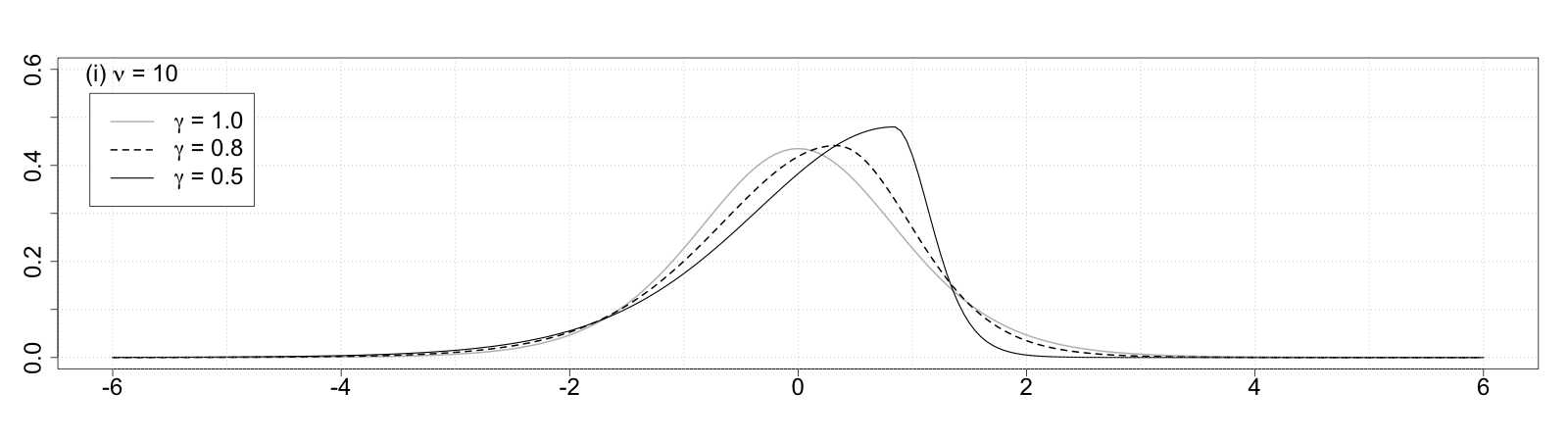
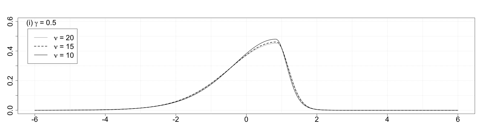
Figure 3: Density function of the standardized FS skew-$t$ distribution defined in (46). (i) $\gamma=1,0.8,0.6$ with $\nu=10$ fixed. (ii) $\nu=20,15,10$ with $\gamma=0.5$ fixed.

3 Bayesian Estimation Methodology

Each of the RSV models defined in Section 2 is characterized as a nonlinear Gaussian state space model with numerous latent variables. This complexity makes the evaluation of the likelihood function, given the parameters, a challenging task, as is the implementation of maximum likelihood estimation. To circumvent these challenges, we adopt a Bayesian approach for parameter estimation using MCMC simulation, as has been done in previous literature.

For the prior distribution of $(\mu,\phi,\sigma_{\eta}^{2},\rho,\xi,\sigma_{u}^{2})$, the parameters common across the RSV models, we assume

$$\mu \sim N(m_{\mu},s_{\mu}^{2}),\quad\frac{\phi+1}{2}\sim B(a_{\phi 0},b_{\phi 0}),$$ (49)

$$\quad\frac{\rho+1}{2} \sim B(a_{\rho 0},b_{\rho 0}),\quad\sigma_{\eta}^{2}\sim IG\left(\frac{n_{\eta}}{2},\frac{S_{\eta}}{2}\right)$$ (50)

$$\xi \sim N(m_{\xi},s_{\xi}^{2}),\quad\sigma_{u}^{2}\sim IG\left(\frac{n_{u}}{2},\frac{S_{u}}{2}\right)$$ (51)

where $B(\cdot,\cdot)$ and $IG(\cdot,\cdot)$ denote beta and inverse gamma distributions, respectively. The parameters of the prior distributions $(m_{\mu},s_{\mu},a_{\phi 0},b_{\phi 0},a_{\rho 0},b_{\rho 0},n_{\eta},S_{\eta},m_{\xi},s_{\xi},n_{u},S_{u})$ are treated as hyperparameters and are chosen to reflect any prior information regarding the parameters.

For notational simplicity, let $\bm{y}=(y_{1},\ldots,y_{n})^{\prime}$, $\bm{x}=(x_{1},\ldots,x_{n})^{\prime}$, and $\bm{h}=(h_{1},\ldots,h_{n})^{\prime}$. Let $\pi(\bm{\theta})$ denote the joint prior probability density of $\bm{\theta}$. Furthermore, let $f(\bm{y},\bm{x},\bm{h}|\bm{\theta})$ denote the likelihood of $(\bm{y},\bm{x})$ given $\bm{\theta}$.

In what follows, we illustrate the MCMC algorithm for the RSV-AZ-ST and RSV-FS-ST models. Additionally, we describe the methodology for obtaining one-day-ahead forecasts of volatility and daily return, from which we derive the one-day-ahead VaR and ES.

3.1 RSV-AZ-ST Model

Let $\bm{\theta}=(\mu,\phi,\rho,\sigma_{\eta}^{2},\delta,\xi,\sigma_{u}^{2},\nu)^{\prime}$, $\bm{\lambda}=(\lambda_{1},\ldots,\lambda_{n})^{\prime}$, and $\bm{z}_{0}=(z_{01},\ldots,z_{0n})^{\prime}$. For the prior distribution of $\bm{\theta}$, excluding $(\mu,\phi,\sigma_{\eta}^{2},\rho,\xi,\sigma_{u}^{2})$, we assume

$$\frac{\delta+1}{2}\sim B(a_{\delta 0},b_{\delta 0}),\quad\nu\sim G(n_{\nu 0},S_{\nu 0}),$$ (52)

where $G(\cdot,\cdot)$ denotes the gamma distribution. We then implement the MCMC simulations as follows.

1. Initialize $\bm{h}$, $\bm{\theta}$, $\bm{z}_{0}$, and $\bm{\lambda}$

2. Generate $\mu|\bm{\theta}_{-\mu},\bm{h},\bm{z}_{0},\bm{\lambda},\bm{x},\bm{y}$

3. Generate $\phi|\bm{\theta}_{-\phi},\bm{h},\bm{z}_{0},\bm{\lambda},\bm{x},\bm{y}$

4. Generate $(\rho,\sigma_{\eta}^{2})|\bm{\theta}_{-(\rho,\sigma_{\eta}^{2})},\bm{h},\bm{z}_{0},\bm{\lambda},\bm{x},\bm{y}$

5. Generate $\delta|\bm{\theta}_{-\delta},\bm{h},\bm{z}_{0},\bm{\lambda},\bm{x},\bm{y}$

6. Generate $\xi|\bm{\theta}_{-\xi},\bm{h},\bm{z}_{0},\bm{\lambda},\bm{x},\bm{y}$

7. Generate $\sigma_{u}^{2}|\bm{\theta}_{-\sigma_{u}^{2}},\bm{h},\bm{z}_{0},\bm{\lambda},\bm{x},\bm{y}$

8. Generate $\nu|\bm{\theta}_{-\nu},\bm{h},\bm{z}_{0},\bm{\lambda},\bm{x},\bm{y}$

9. Generate $\bm{z}_{0}|\bm{\theta},\bm{h},\bm{\lambda},\bm{x},\bm{y}$

10. Generate $\bm{h}|\bm{\theta},\bm{z}_{0},\bm{\lambda},\bm{x},\bm{y}$

11. Generate $\bm{\lambda}|\bm{\theta},\bm{h},\bm{z}_{0},\bm{x},\bm{y}$

12. Return to step 2

The specific details for each sampling scheme are provided in Appendix A.1.

3.2 RSV-FS-ST Model

Let $\bm{\theta}=(\mu,\phi,\rho,\sigma_{\eta}^{2},\gamma,\xi,\sigma_{u}^{2},\nu)^{\prime}$. For the prior distribution of $\bm{\theta}$, excluding $(\mu,\phi,\sigma_{\eta}^{2},\rho,\xi,\sigma_{u}^{2})$, we assume

$$\gamma\sim G(n_{\gamma 0},S_{\gamma 0}),\quad\nu\sim G(n_{\nu 0},S_{\nu 0}).$$ (53)

We then implement the MCMC simulations as follows.

1. Initialize $\bm{h}$ and $\bm{\theta}$.

2. Generate $\mu|\bm{\theta}_{-\mu},\bm{h},\bm{x},\bm{y}$.

3. Generate $\phi|\bm{\theta}_{-\phi},\bm{h},\bm{x},\bm{y}$.

4. Generate $\rho|\bm{\theta}_{-\rho},\bm{h},\bm{x},\bm{y}$.

5. Generate $\sigma_{\eta}^{2}|\bm{\theta}_{-\sigma_{\eta}^{2}},\bm{h},\bm{x},\bm{y}$.

6. Generate $\xi|\bm{\theta}_{-\xi},\bm{h},\bm{x},\bm{y}$.

7. Generate $\sigma_{u}^{2}|\bm{\theta}_{-\sigma_{u}^{2}},\bm{h},\bm{x},\bm{y}$.

8. Generate $\gamma|\bm{\theta}_{-\gamma},\bm{h},\bm{x},\bm{y}$.

9. Generate $\nu|\bm{\theta}_{-\nu},\bm{h},\bm{x},\bm{y}$.

10. Generate $\bm{h}|\bm{\theta},\bm{x},\bm{y}$.

11. Return to step 2

The specific details for each sampling scheme are provided in Appendix A.2.

3.3 One-day-ahead Forecast

To obtain one-day-ahead forecasts of financial returns and volatilities, we utilize the predictive distribution within each state-space model. Let $\bm{\theta}^{(i)}$ and $\bm{h}^{(i)}$ represent the $i$th sample of parameters and latent log-volatilities in the MCMC simulation, respectively. We can then generate the one-step-ahead predictive samples as follows.

1. Generate $h_{n+1}^{(i)}|\bm{x},\bm{y},\bm{h}^{(i)},\bm{\theta}^{(i)}\sim N(\mu_{n+1}^{(i)},(\sigma_{n+1}^{(i)})^{2})$ where

   $$\mu_{n+1}^{(i)} =\mu^{(i)}+\phi^{(i)}h_{n}^{(i)}-\mu^{(i)}+\rho^{(i)}\sigma_{\eta}^{(i)}y_{n}\exp\left(-\frac{h_{n}^{(i)}}{2}\right),$$ (54)

   $$(\sigma_{n+1}^{(i)})^{2} =(1-(\rho^{(i)})^{2})(\sigma_{\eta}^{(i)})^{2}.$$ (55)

2. Generate $\epsilon_{n+1}^{(i)}$ from the distribution corresponding to the chosen RSV model given $\bm{\theta}^{(i)}$ and $\bm{h}^{(i)}$.

3. Compute $y_{n+1}^{(i)}$ as

   $$y_{n+1}^{(i)}=\epsilon_{n+1}^{(i)}\exp\left(-\frac{h_{n+1}^{(i)}}{2}\right).$$ (56)

By repeating the above procedure for $M$ times, we obtain the generated samples $\{h_{n+1}^{(i)}\}_{i=1}^{M}$ and $\{y_{n+1}^{(i)}\}_{i=1}^{M}$.

One-day-ahead quantile forecasts, such as VaR and ES, can be derived from the distribution of $\{y_{n+1}^{(i)}\}_{i=1}^{M}$ for each model. The one-day-ahead VaR forecasts with probability $\alpha$ at time $n+1$, denoted by $\mbox{VaR}_{n+1}(\alpha)$, are defined as

$$\mbox{Pr}(y_{n+1}<\mbox{VaR}_{n+1}(\alpha)|\mathcal{I}_{n})=\alpha,$$ (57)

where $\mathcal{I}_{n}$ denotes the information set available at time $n$. The corresponding ES forecasts, denoted by $\mbox{ES}_{n+1}(\alpha)$, are then given as

$$\mbox{ES}_{n+1}(\alpha)=E[y_{n+1}|y_{n+1}<\mbox{VaR}_{n+1}(\alpha),\mathcal{I}_{n}]$$ (58)

The one-day-ahead VaR and ES can be obtained as the $(1-\alpha)$th quantile and conditional average of $\{y_{n+1}^{(i)}\}_{i=1}^{M}$, respectively.

We evaluate the obtained volatility, VaR, and ES forecasts by employing suitable loss or scoring functions. Specifically, following Takahashi et al. (2023), we compute the Mean Squared Error (MSE) and Gaussian Quasi-Likelihood (QLIKE) loss functions for volatility forecasts, and the Fissler and Ziegel (2016) (FZ) joint loss function for VaR and ES forecasts. To utilize the FZ loss function for forecast evaluation, we adhere to Patton et al. (2019) and employ the following form, referred to as the FZ0 loss function hereafter,

$$L_{FZ0}(y,v,e;\alpha)=-\frac{1}{\alpha e}\mathbbm{1}\{y\leq v\}(v-y)+\frac{v}{e}+\log(-e)-1,$$ (59)

where $y$, $v$, and $e$ denote a return, VaR, and ES, respectively. Patton et al. (2019) demonstrate that the FZ0 loss function is the only FZ loss function generating loss differences that are homogeneous of degree zero.

While average losses derived from the aforementioned loss functions offer initial insights into the forecast performance of the models in contention, they do not indicate if the differences in losses are statistically significant. To ascertain this, we utilize the conditional and unconditional predictive ability tests by Giacomini and White (2006), hereinafter referred to as GW tests, on the loss differences. The GW tests are particularly pertinent to this paper’s objectives because they emphasize the rolling window methods we adopt in Section 4. This allows for a cohesive assessment of both nested and non-nested models, including the RSV models described in Section 2.

For the unconditional predictive ability, the GW test statistic conforms to that proposed by Diebold and Mariano (2002) and is, under the null hypothesis, asymptotically standard normally distributed. For the conditional predictive ability, the GW test defines the null hypothesis as

$$H_{0,h}:E[\Delta L_{t+1}|\mathcal{I}_{t}]=0,\quad t=n,n+1,\ldots,n+n_{f}-1,$$ (60)

where $\Delta L_{t}$ is the loss difference between two models at forecast date $t$, and $\mathcal{I}_{t}$ is the information set at time $t$.

Given a test function $\mathbbm{h}_{t}$, a $q\times 1$ vector measurable with respect to $\mathcal{I}_{t}$ (Stinchcombe and White, 1998), the null hypothesis translates to

$$H_{0,h}:E[\mathbbm{h}_{t}\Delta L_{t+1}]=0,\quad t=n,n+1,\ldots,n+n_{f}-1.$$ (61)

Defining $Z_{t+1}=\mathbbm{h}_{t}\Delta L_{t+1}$ and $\bar{Z}_{n_{f}}=n_{f}^{-1}\sum_{t=n}^{n+n_{f}-1}Z_{t+1}$, the alternative hypothesis becomes

$$H_{A,h}:E[\bar{Z}_{n_{f}}^{\prime}]E[\bar{Z}_{n_{f}}]\geq d>0,\quad\mbox{for sufficiently large $n_{f}$}.$$ (62)

We employ the Wald-type test statistic

$$T_{n_{f}}=n\bar{Z}_{n_{f}}^{\prime}\hat{\Omega}_{n_{f}}^{-1}\bar{Z}_{n_{f}},$$ (63)

where $\hat{\Omega}_{n_{f}}=n_{f}^{-1}\sum_{t=n}^{n+n_{f}-1}Z_{t+1}Z_{t+1}^{\prime}$ consistently estimates the variance of $Z_{t+1}$. Under the null, $T_{n_{f}}$ follows a chi-square distribution with $q$ degrees of freedom, $\chi_{q}^{2}$. For significance level $p$, the null hypothesis is rejected when $T_{n_{f}}>\chi_{q,1-p}^{2}$, where $\chi_{q,1-p}^{2}$ is the $(1-p)$ quantile of $\chi_{q}^{2}$.

In practice, the selection of $\mathbbm{h}_{t}$ should discern between the forecast performances of the models. Focusing on one-day-ahead forecasts, we follow the specifications of Takahashi et al. (2023) and define $\mathbbm{h}_{t}=(1,\Delta L_{t})^{\prime}$ for $t=n,n+1,\ldots,n+n_{f}-1$. If the null is rejected, it implies that the lagged loss differences, $\Delta L_{t}$, can forecast the subsequent loss differences, $\Delta L_{t+1}$. Using $\hat{b}$ to represent the regression coefficient of $\Delta L_{t+1}$ on $\mathbbm{h}_{t}$, the predicted loss differences $\{\hat{b}^{\prime}\mathbbm{h}_{t}\}_{t=n}^{n+n_{f}-1}$ serve as indicators for assessing model performances across different time points. In Section 4, we measure relative performance by the frequency with which one model forecasts larger losses than the other, as expressed by

$$I_{n_{f},0}=\frac{1}{n_{f}}\sum_{t=n}^{n+n_{f}-1}I(\hat{b}^{\prime}\mathbbm{h}_{t}>0).$$ (64)

4 Empirical Study

4.1 Data and Descriptive Statistics

We implement the SV and RSV models, as described in Section 2, on the daily (close-to-close) returns and Realized Volatilities (RVs) of the U.S. and Japanese stock indices, Dow Jones Industrial Average (DJIA) and Nikkei 225 (N225). Following Liu et al. (2015), we employ a 5-minute RV, computed excluding the non-trading hours, among various RV estimators. The DJIA data are sourced from the Oxford-Man Institute’s Realized Library (https://realized.oxford-man.ox.ac.uk/), while the N225 data are derived from the Nikkei NEEDS-TICK dataset. The analysis spans from June 2009 to September 2019 for both indices. Specifically, the DJIA sample encompasses 2,596 trading days from June 1, 2009, to September 27, 2019, and the N225 sample covers 2,532 trading days from June 1, 2009, to September 30, 2019.

Figure 4 displays the time series plots and histograms of the daily returns for DJIA and N225. We notice that the daily returns fluctuate considerably around zero for both series. Additionally, the returns tend to exhibit larger values in the negative direction, indicating a negative skewness.

DJIA	N225

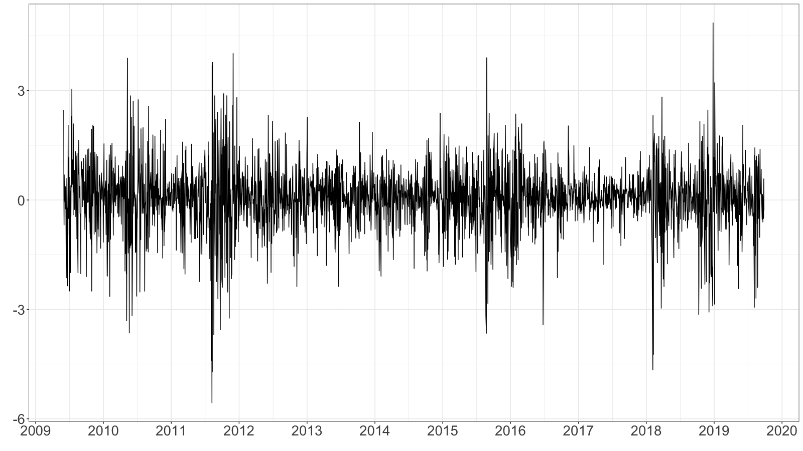
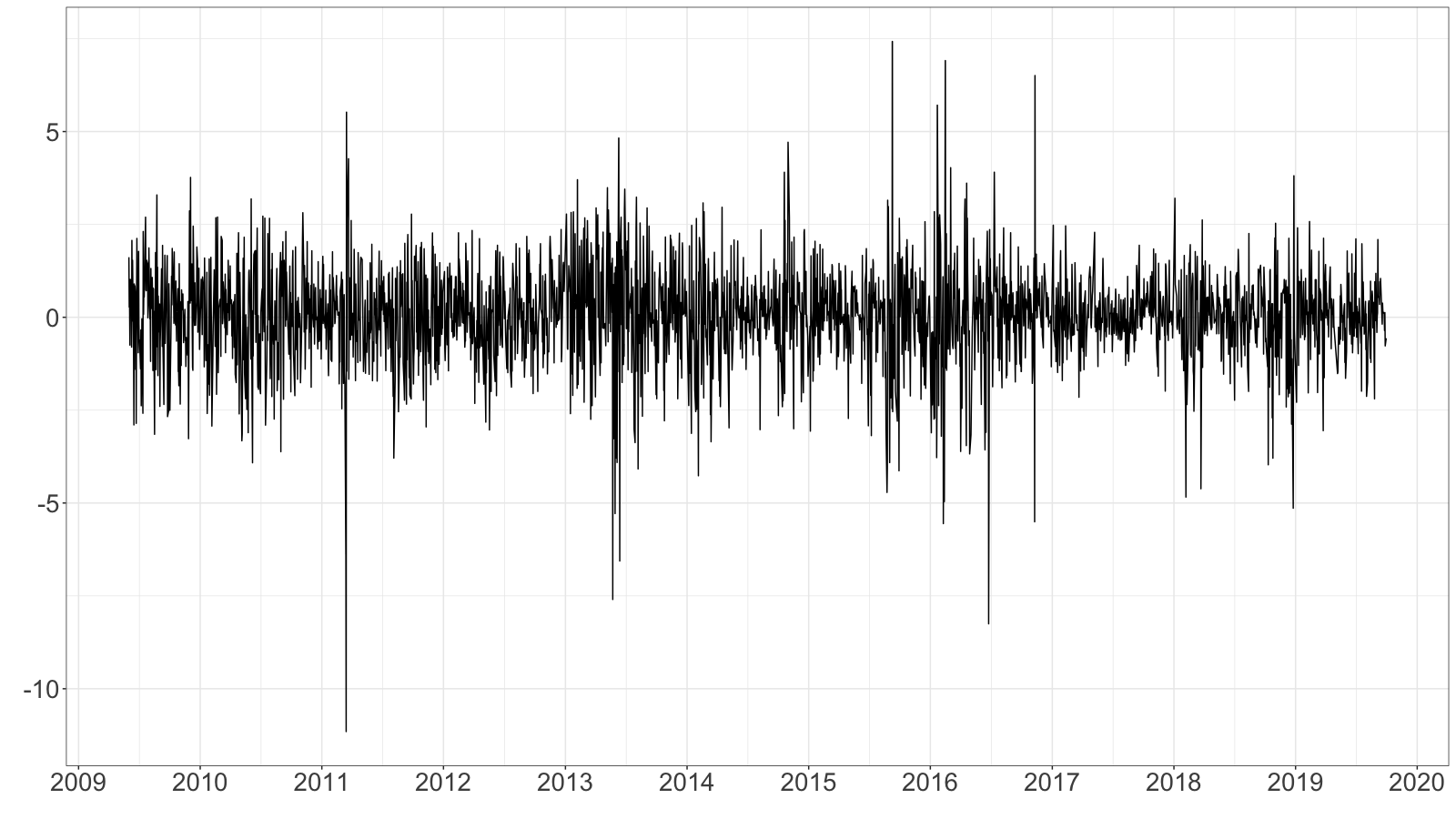
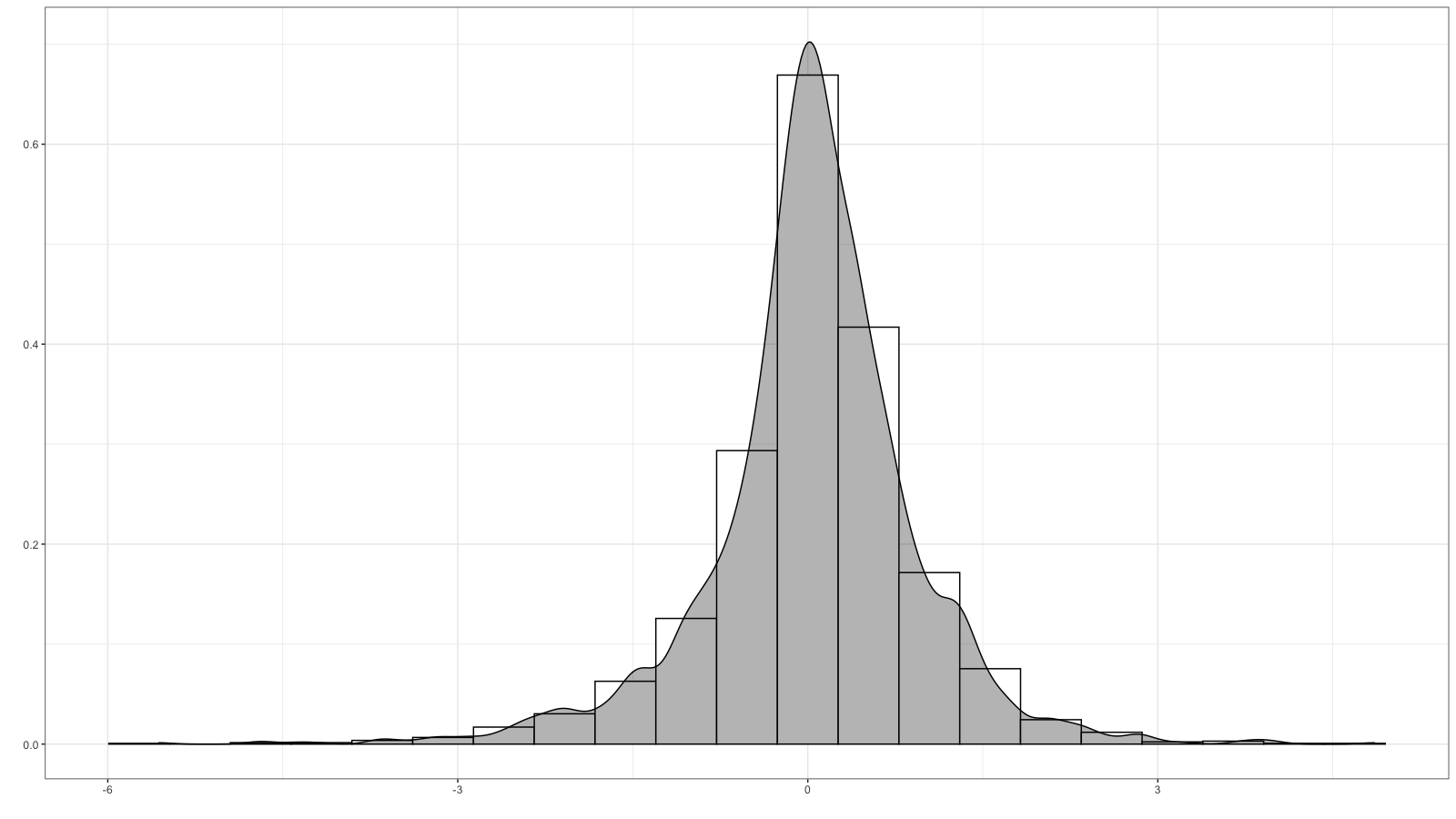
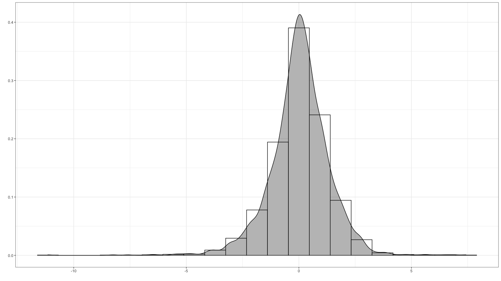
Figure 4: Time series plots (top) and histograms (bottom) of the daily returns in percentage points for DJIA and N225.

Table 1 displays the descriptive statistics of the daily returns. For DJIA, the means of daily returns significantly deviate from zero, while for N225, they do not. Given the minuscule magnitude of the mean, we opt not to adjust the mean of daily returns for both series in subsequent analyses. The $p$-value of the Ljung and Box (1978) statistic, modified for heteroskedasticity following Diebold (1988) to examine the null hypothesis of no autocorrelation up to 10 lags, suggests that the null hypothesis stands unrejected. This result enables us to estimate the models utilizing the daily returns without making adjustments for the autocorrelation. The kurtosis of daily returns highlights a leptokurtic distribution, a characteristic commonly observed in financial returns, and the skewness of daily returns is significantly negative for both series. Consequently, the Jarque-Bera (JB) statistic repudiates its normality. The excess kurtosis and negative skewness are anticipated to be accounted for by adopting the skew-$t$ distributions detailed in Section 2 for daily returns.

Table 1: Descriptive statistics of the daily returns for DJIA and N225

	Mean	SD	Skew	Kurt	Min	Max	JB	LB
DJIA	$0.044$	$0.895$	$-0.448$	$6.675$	$-5.562$	$4.857$	$0.00$	$0.52$
	$(0.018)$		$(0.048)$	$(0.096)$
N225	$0.033$	$1.321$	$-0.544$	$8.101$	$-11.153$	$7.426$	$0.00$	$0.55$
	$(0.026)$		$(0.049)$	$(0.097)$

Note: Parenthetical figures indicate standard errors. JB denotes the $p$-value of the Jarque-Bera statistic. LB refers to the $p$-value of the Ljung and Box (1978) statistic, adapted as per Diebold (1988).

Figure 5 illustrates the time series plots of the 5-minute RVs alongside their logarithms, as well as histograms for DJIA and N225. The RVs exhibit substantial variance, occasional clusters, and some pronounced spikes for both series. Such sporadic large values of RVs lead to a positive skew in their logarithms.

DJIA	N225

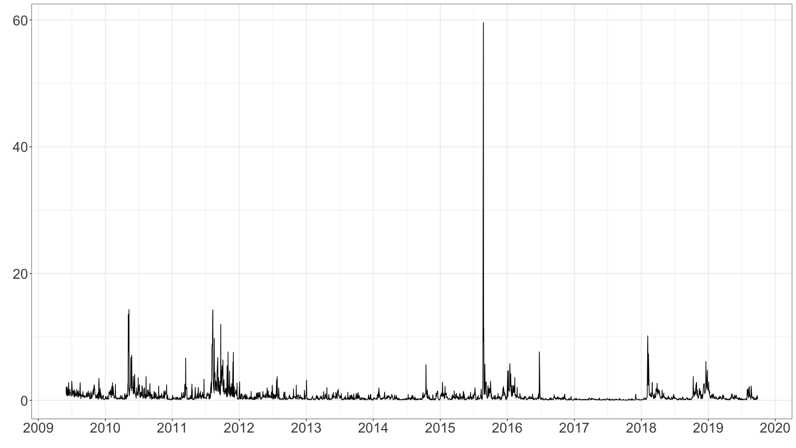
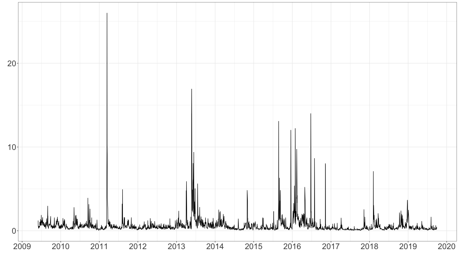
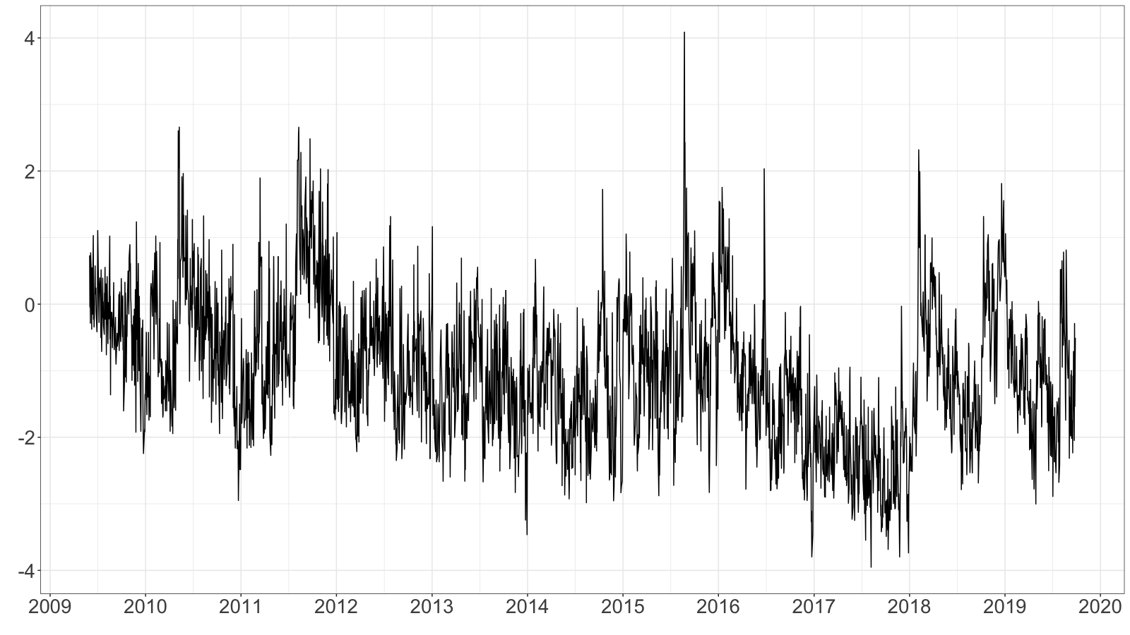
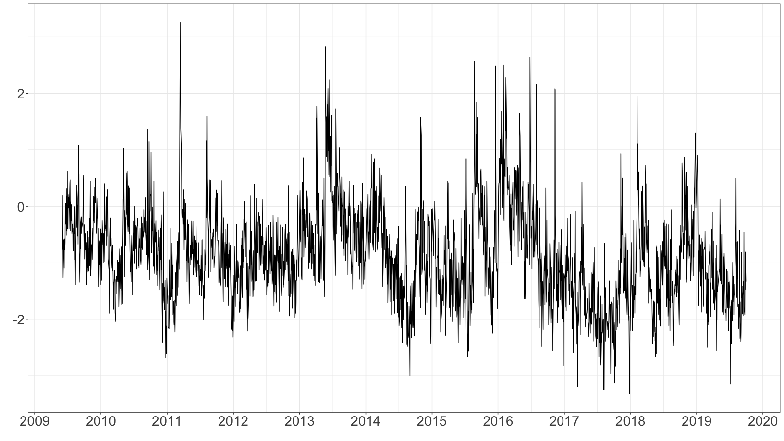
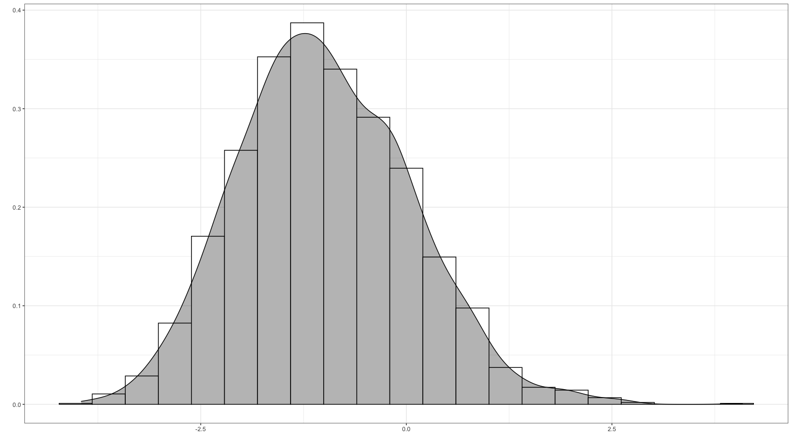
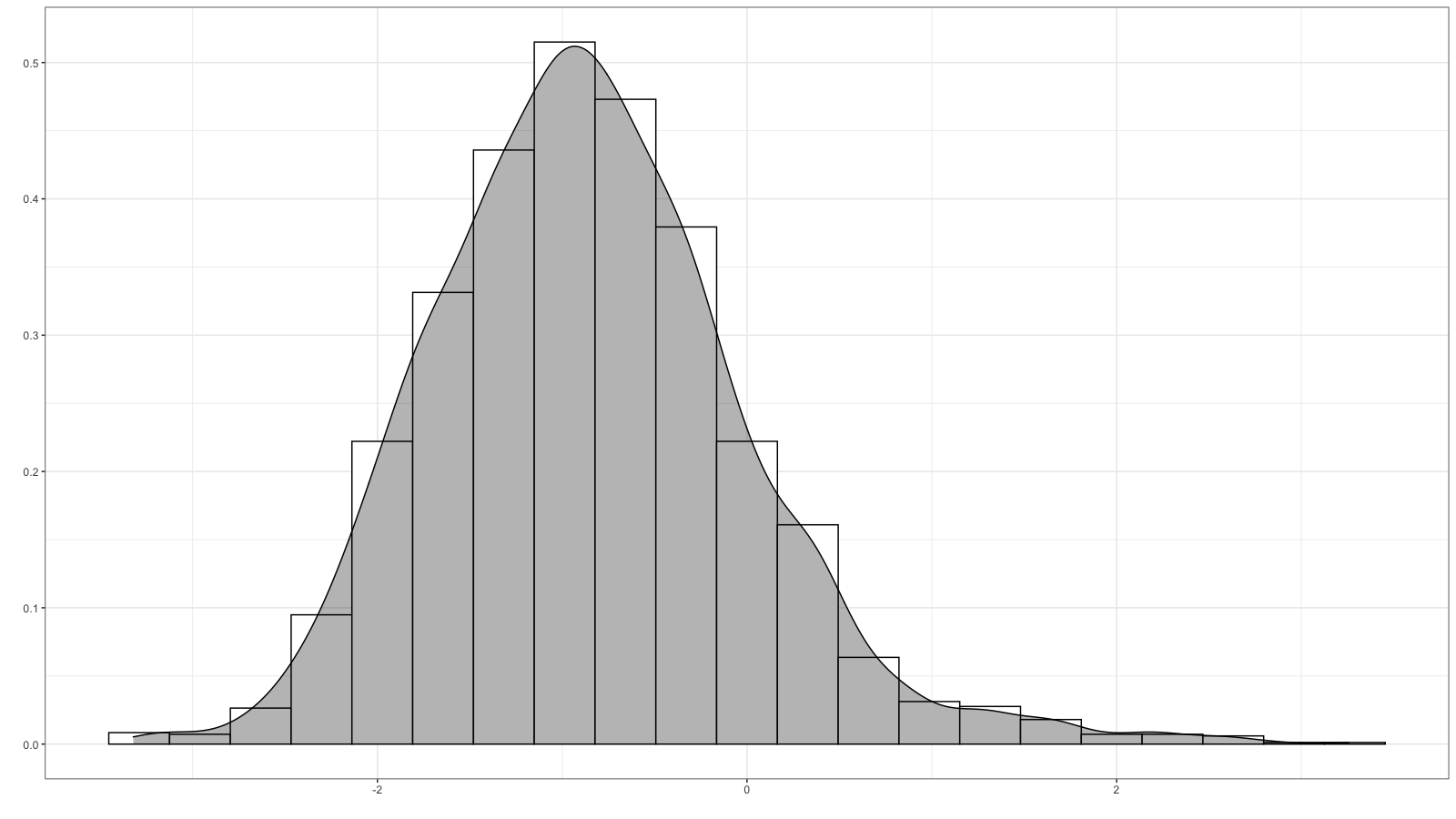
Figure 5: Time series plots of 5-minute RVs (top) and their logarithms (middle), along with histograms of the logarithms (bottom) for DJIA and N225.

Table 2 delineates the descriptive statistics of the 5-minute RVs and their logarithms. For both DJIA and N225, the LB statistic repudiates the null hypothesis of no autocorrelation, aligning with the widely acknowledged persistence of volatility termed as volatility clustering. The skewness is markedly positive, and the kurtosis indicates a leptokurtic distribution. Consequently, the JB statistic refutes the normality of the logarithms of 5-minute RVs. This refutation contradicts the assumed normality of the error term $u_{t}$ in the RSV model denoted by equation (16), albeit we adhere to this assumption herein. Addressing the non-normality within the model emerges as a compelling avenue for prospective research.

Table 2: Descriptive statistics of the logarithms of 5-minute RVs for DJIA and N225

	Mean	SD	Skew	Kurt	Min	Max	JB	LB
DJIA	$-0.987$	$1.048$	$0.317$	$3.177$	$-3.953$	$4.087$	$0.00$	$0.00$
	$(0.021)$		$(0.048)$	$(0.096)$
N225	$-0.858$	$0.844$	$0.589$	$4.219$	$-3.321$	$3.258$	$0.00$	$0.00$
	$(0.017)$		$(0.049)$	$(0.097)$

Note: Refer to Table 1 for additional details.

4.2 Competing Models

We evaluate the forecast performance of the RSV models as outlined below:

1. RSV-N: RSV model in which $\epsilon_{t}$ follows a normal distribution.

2. RSV-T: RSV model in which $\epsilon_{t}$ follows Student’s $t$ distribution.

3. RSV-GH-ST: RSV model in which $\epsilon_{t}$ follows the GH skew-$t$ distribution.

4. RSV-AZ-SN: RSV model in which $\epsilon_{t}$ follows the AZ skew normal distribution.

5. RSV-AZ-ST: RSV model in which $\epsilon_{t}$ follows the AZ skew-$t$ distribution.

6. RSV-FS-SN: RSV model in which $\epsilon_{t}$ follows the FS skew normal distribution.

7. RSV-FS-ST: RSV model in which $\epsilon_{t}$ follows the FS skew-$t$ distribution.

We set the priors for the standard parameters as follows

$$\mu\sim N(0,100),\quad\frac{\phi+1}{2}\sim B(1,1),\quad\frac{\rho+1}{2}\sim B(1,1),\quad\sigma_{\eta}^{2}\sim IG(0.05,0.05),$$ (65)

$$\xi\sim N(0,10),\quad\sigma_{u}^{2}\sim IG(2.5,0.1).$$ (66)

And for the remaining parameters, we have

$$\nu\sim G(5,0.5),\quad\beta\sim N(0,1),\quad\frac{\delta+1}{2}\sim B(1,1),\quad\gamma\sim G(1,1).$$ (67)

Considering that GARCH models—including ARCH (Engle, 1982), GARCH (Bollerslev, 1986), and their extensions—are frequently employed to capture time-varying volatility, we assess the efficacy of RSV models by contrasting them with GARCH and SV models. From the myriad of GARCH models available, we select the EGARCH model as introduced by Nelson (1988). Incorporating RV, both Hansen et al. (2012) and Hansen and Huang (2016) extended the GARCH and EGARCH models, respectively. Given that the REGARCH model is a more comprehensive version than the RGARCH, we opt for the REGARCH model. For model descriptions, see Takahashi et al. (2023), for instance.

In our out-of-sample forecasting, we adopt the standard normal and Student’s $t$ distributions for returns. We then estimate these models’ parameters using the QML method and predict the one-day-ahead volatility, VaR, and ES forecasts by integrating the QML estimates into the parameters. For other realized GARCH models employing Bayesian estimation techniques and their applications to volatility, VaR, and ES forecasts, refer to Chen et al. (2021).

4.3 Out-of-sample Forecasting

Adhering to the approach of Takahashi et al. (2016), we employ a rolling window estimation strategy to forecast volatility, VaR, and ES. The window size remains constant throughout the analysis. For the DJIA, this size is set at 1,993 observations, with the last observation dates spanning from April 28, 2017, to September 26, 2019. For the N225, the window encompasses 1,942 observations, and the final observation dates range from April 28, 2017, to September 27, 2019. We produce one-day ahead forecasts after each estimation. Specifically, we generate 15,000 prediction samples, then calculate the means and medians of volatility forecasts for the SV and RSV models. Additionally, we compute the quantiles of return forecasts. Ultimately, from the start of May 2017 to the close of September 2019, we amass 603 and 590 prediction samples for the DJIA and N225, respectively.

4.3.1 Volatility forecasts

To appraise the accuracy of the volatility forecasts, we compute their average loss using the MSE and QLIKE loss metrics, as elaborated in Section 3.3. Both the MSE and QLIKE losses are robust functions and offer rankings congruent with those derived using the true volatility, provided the volatility proxy serves as a conditionally unbiased estimator of the actual volatility. In order to counteract the bias introduced by market microstructure noise, we employ the RK utilizing the Parzen kernel function, accompanied by a bandwidth as recommended by Barndorff-Nielsen et al. (2009), to approximate the underlying volatility. Additionally, to correct for biases arising from non-trading hours, we adopt the method proposed by Hansen and Lunde (2005), adjusting the influence of these non-trading periods on the RK according to equation (9). Specifically, the adjustment term $c_{HL}$ for the RK at time $t$ is computed as

$$c_{HL}=\frac{\sum_{s=t-n+1}^{t}(y_{s}-\bar{y})^{2}}{\sum_{s=t-n+1}^{t}RK_{s}},\quad\bar{y}=\frac{1}{n}\sum_{s=t-n+1}^{t}y_{s},$$ (68)

where $n$ signifies the fixed window size.

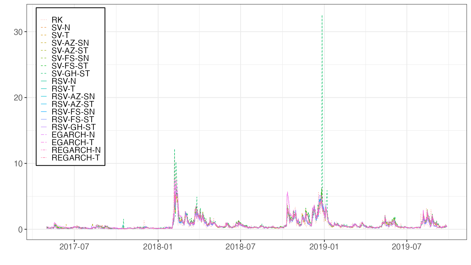
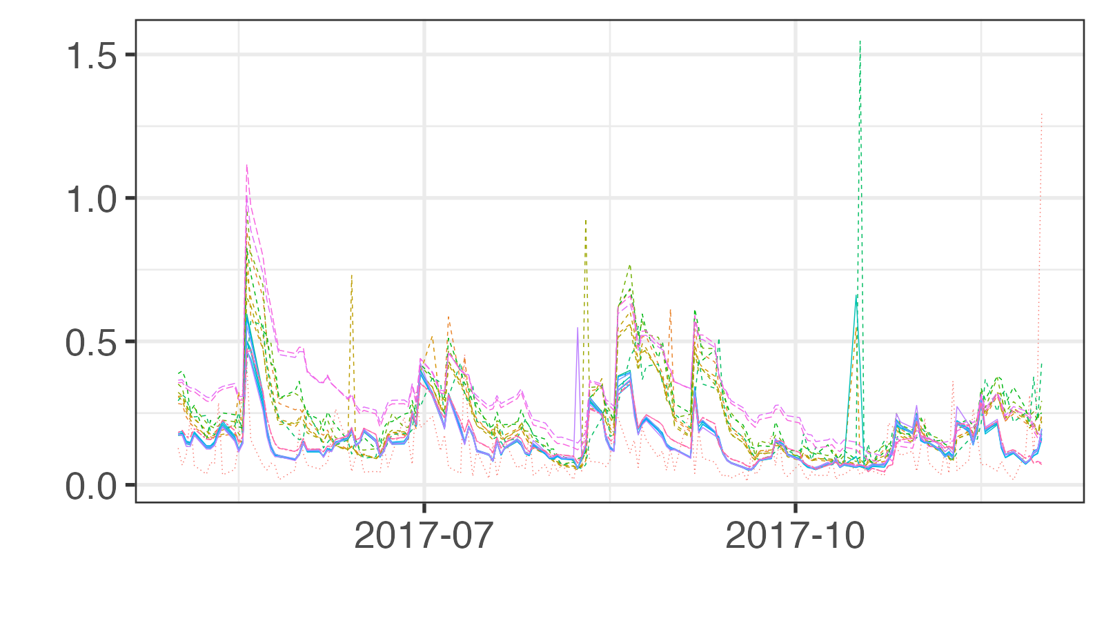
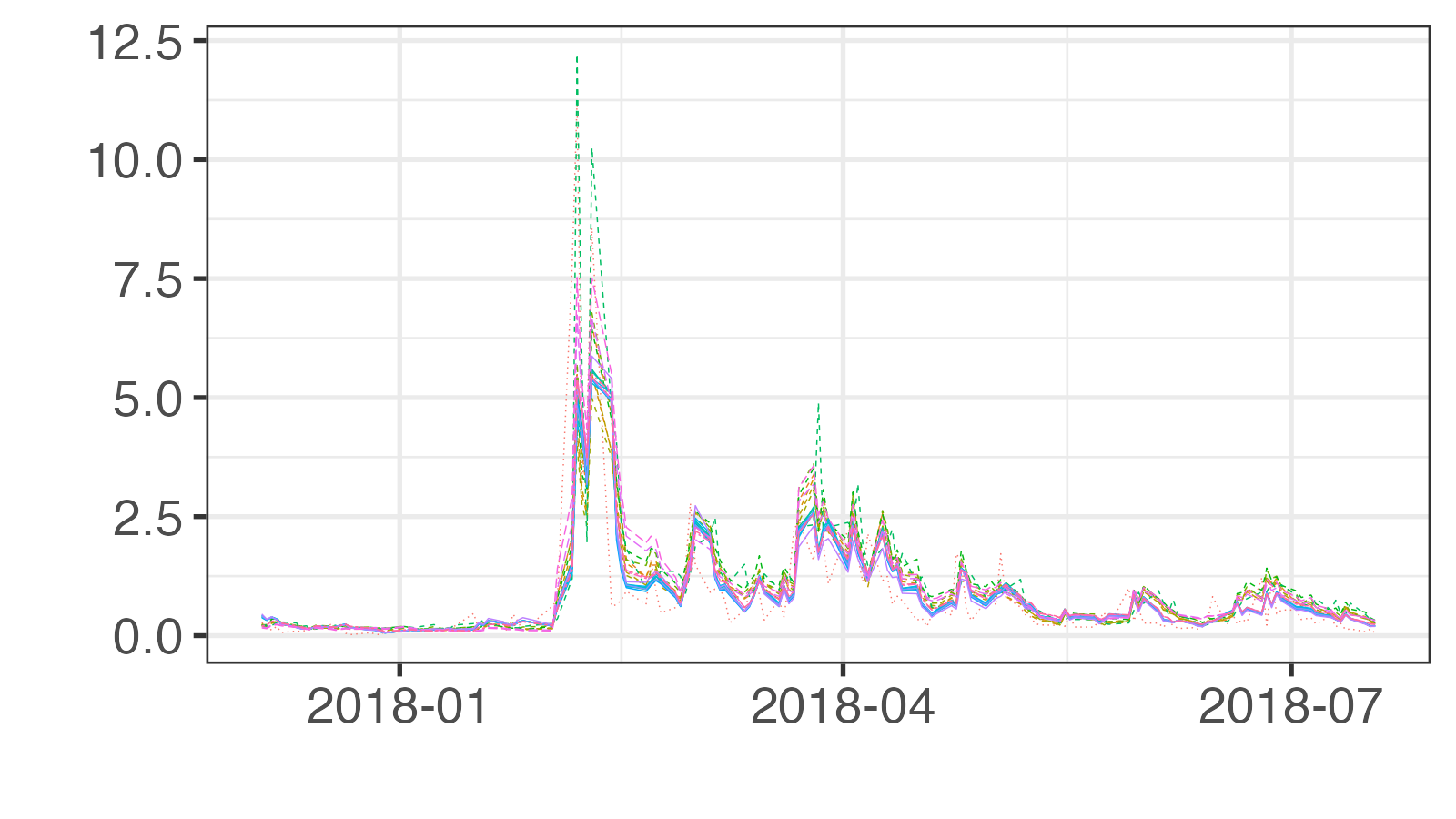
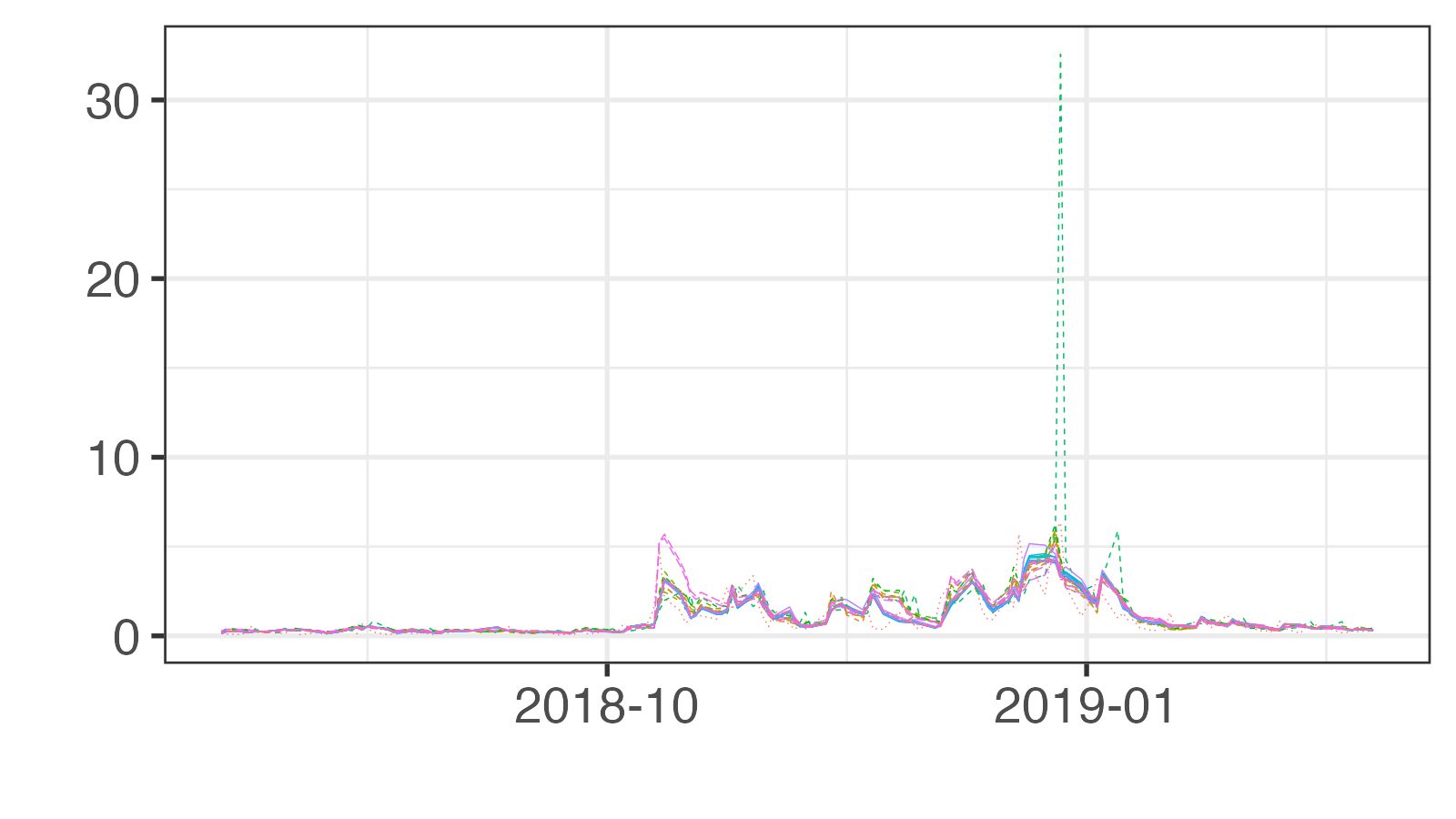
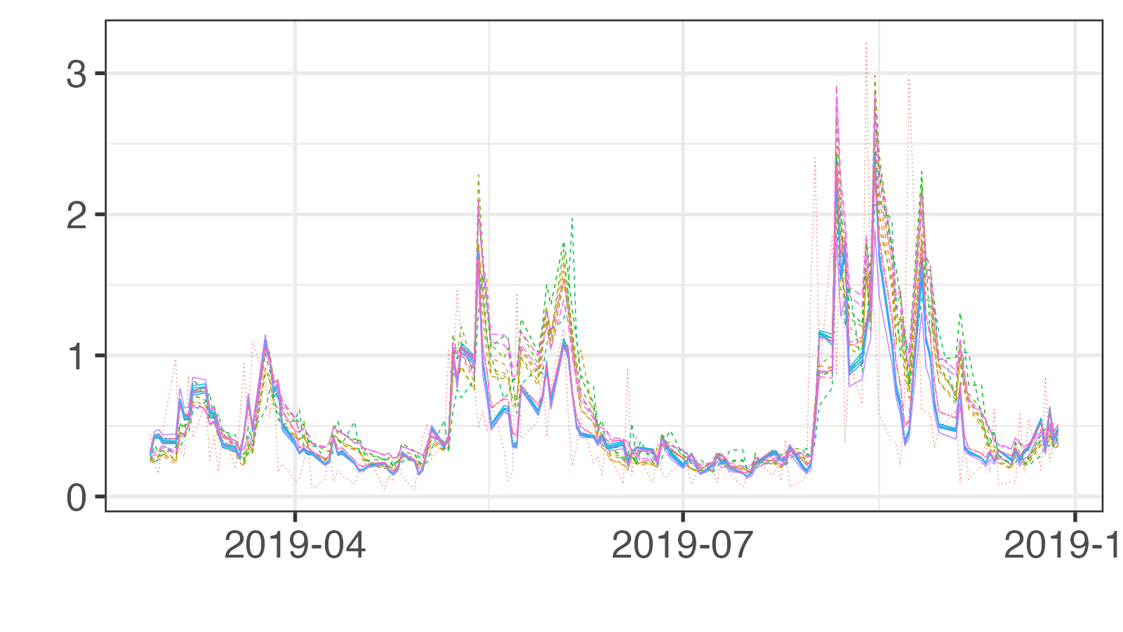
Figure 6: Volatility forecasts and adjusted RKs for DJIA: Overall period (top) and sub-periods (bottom).

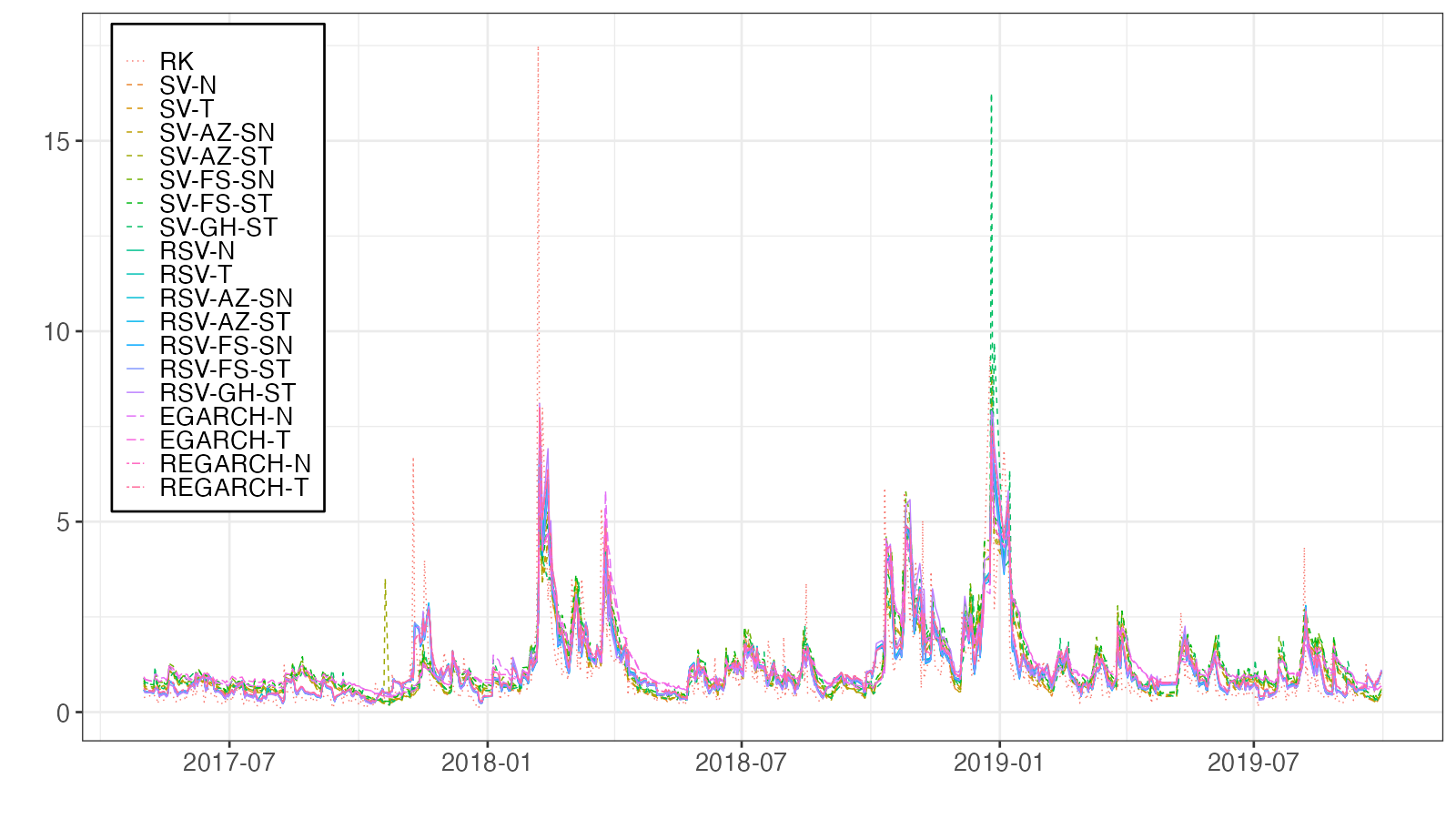
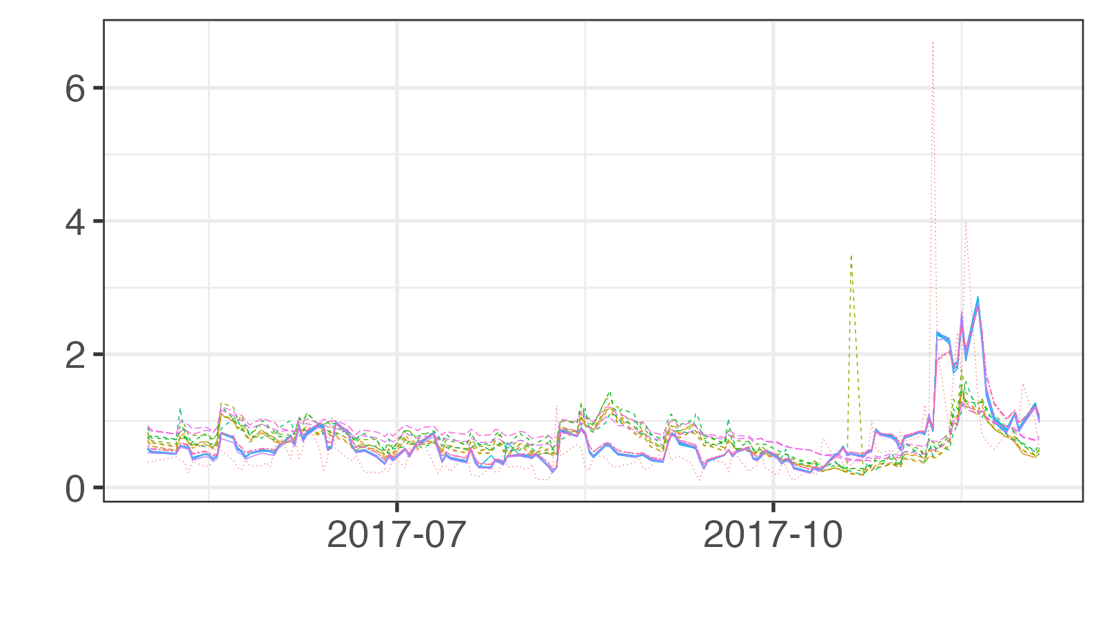
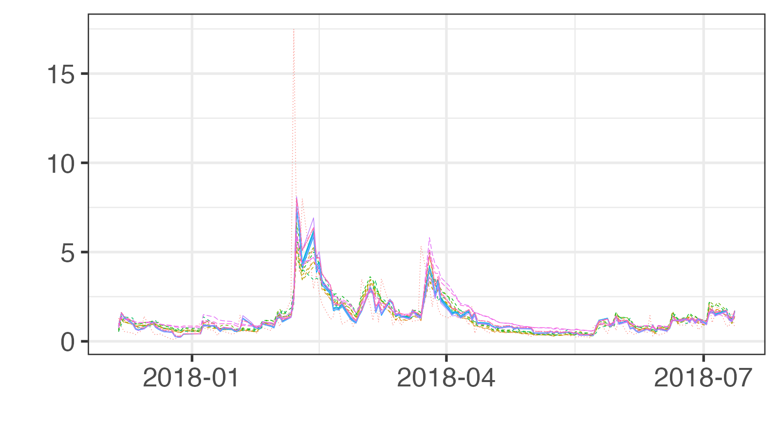
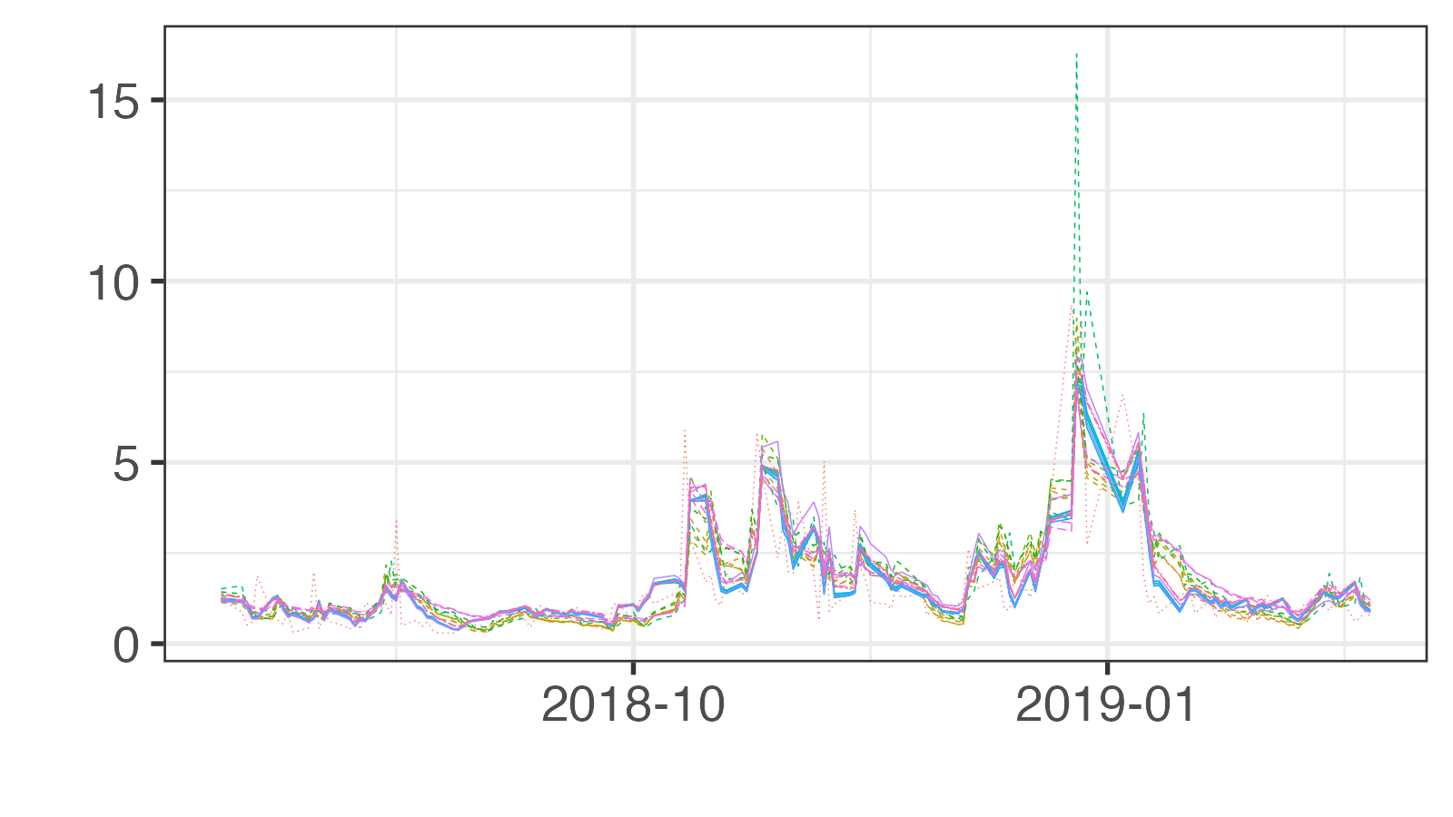
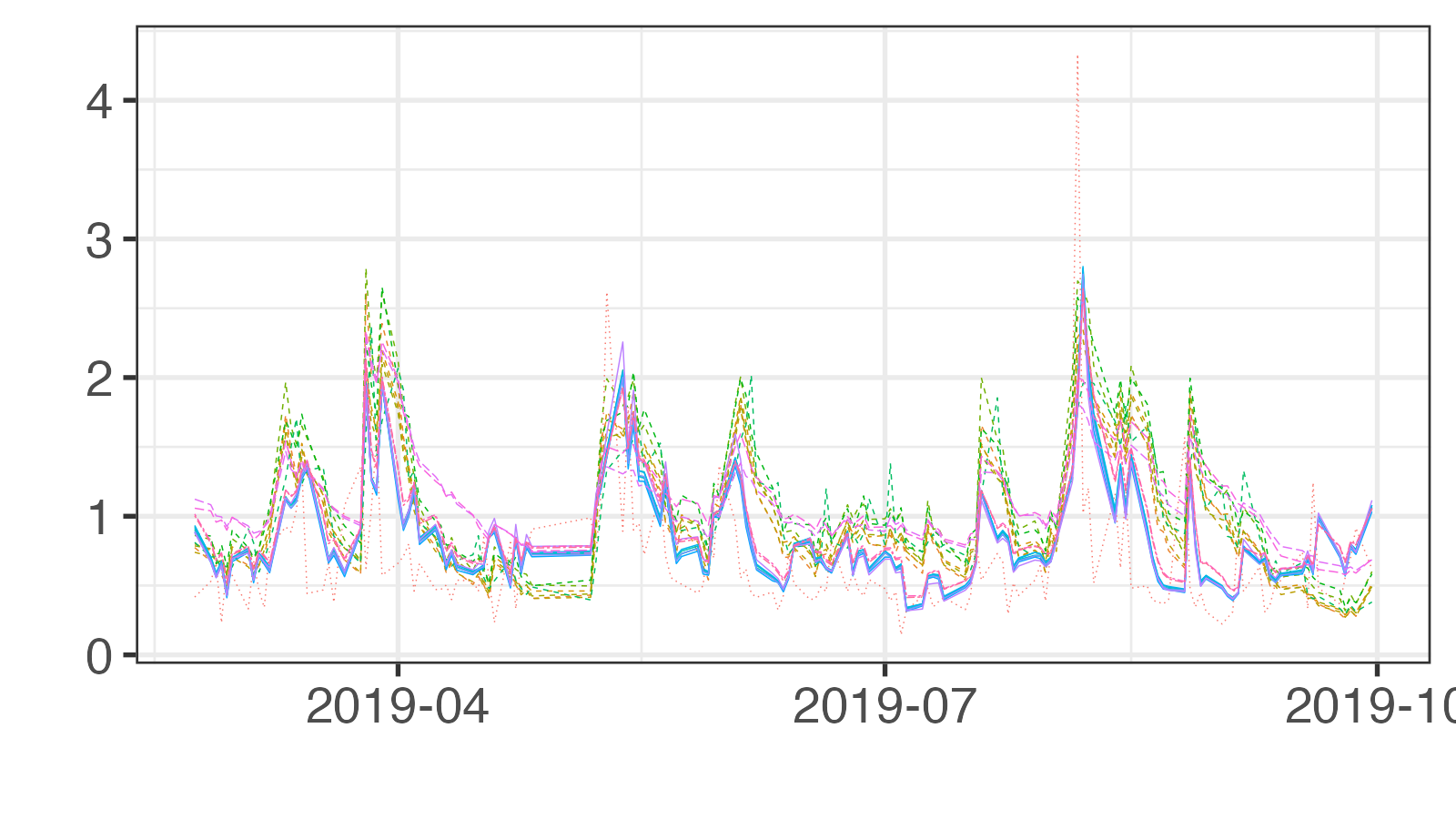
Figure 7: Volatility forecasts and adjusted RKs for N225: Overall period (top) and sub-periods (bottom).

Figure 6 displays the volatility forecasts alongside the adjusted RKs for DJIA. We note that the forecasts from the SV models present several spikes. Notably, the SV-GH-ST model significantly over-predicts the volatility towards the end of 2018 relative to other models. The general observation suggests that the volatility forecasts from the RSV models tend to be more accurate (closer to the RK) compared to the SV models, highlighting the enhancing role of RV in prediction accuracy. Figure 7 depicts analogous observations for the N225.

Table 3 presents the average losses of volatility forecasts for DJIA along with the $p$-values of the model confidence set (MCS) proposed by Hansen et al. (2011). The RSV-FS-SN model yields the lowest MSE and QLIKE scores. With ^∗∗ and ^∗ denoting models within the 75% and 90% MCS, respectively, we generally find that the volatility forecasts of the RSV and REGARCH models surpass those of the SV and EGARCH models. Moreover, the MSE for the SV-GH-ST model is substantially higher than for other models, echoing the over-prediction of volatility towards the end of 2018. It is essential to note that the MSE and QLIKE are loss functions with homogeneous degrees of 1 and 0, respectively. As a result, the QLIKE for the SV-GH-ST model is higher than for other models but to a lesser degree.

Table 3: Average losses of volatility forecasts for DJIA

	MSE	$p_{MCS}$	QLIKE	$p_{MCS}$
SV-N	$0.2132$	$1.00^{**}$	$0.3019$	$0.00^{\hskip 5.60002pt}$
SV-T	$0.2280$	$1.00^{**}$	$0.2990$	$0.00^{\hskip 5.60002pt}$
SV-AZ-SN	$0.2085$	$1.00^{**}$	$0.2951$	$0.00^{\hskip 5.60002pt}$
SV-AZ-ST	$0.2251$	$1.00^{**}$	$0.2932$	$0.00^{\hskip 5.60002pt}$
SV-FS-SN	$0.2263$	$1.00^{**}$	$0.3243$	$0.00^{\hskip 5.60002pt}$
SV-FS-ST	$0.2445$	$1.00^{**}$	$0.3327$	$0.00^{\hskip 5.60002pt}$
SV-GH-ST	$0.8092$	$0.50^{**}$	$0.3213$	$0.00^{\hskip 5.60002pt}$
RSV-N	$0.2075$	$1.00^{**}$	$0.2526$	$1.00^{**}$
RSV-T	$0.2156$	$1.00^{**}$	$0.2587$	$1.00^{**}$
RSV-AZ-SN	$0.2168$	$1.00^{**}$	$0.2538$	$1.00^{**}$
RSV-AZ-ST	$0.2214$	$1.00^{**}$	$0.2563$	$1.00^{**}$
RSV-FS-SN	$0.2069$	$1.00^{**}$	$0.2516$	$1.00^{**}$
RSV-FS-ST	$0.2109$	$1.00^{**}$	$0.2541$	$1.00^{**}$
RSV-GH-ST	$0.2137$	$1.00^{**}$	$0.2567$	$1.00^{**}$
EGARCH-N	$0.2207$	$1.00^{**}$	$0.3580$	$0.00^{\hskip 5.60002pt}$
EGARCH-T	$0.2359$	$1.00^{**}$	$0.3615$	$0.00^{\hskip 5.60002pt}$
REGARCH-N	$0.2100$	$1.00^{**}$	$0.2767$	$0.28^{**}$
REGARCH-T	$0.2133$	$1.00^{**}$	$0.2794$	$0.29^{**}$

Notes: $p_{MCS}$ denotes the MCS $p$-value. ^∗∗ and ^∗ represent models within the 75% and 90% MCS, respectively.

The outcomes of the GW tests on the loss differences can be found in Table 4. The lower triangular sections of the table provide the test statistics for the unconditional GW test. A negative value in this context signifies that the row model outperforms the column model. Conversely, the upper triangular sections display the percentage of predicted losses stemming from the conditional GW test, as delineated in (64). In this case, a higher percentage indicates superior performance by the column model compared to the row model. Significance of the GW tests’ rejection is marked by symbols ^∗ and ^∗∗ for the 1% and 5% levels, respectively. Our evaluation reveals the RSV models notably outperforming the SV and EGARCH models. The REGARCH models, meanwhile, show improved performance over the EGARCH models, underscoring the benefits of incorporating RV into volatility forecasts. Furthermore, the superiority of the SV models over the EGEARCH models is consistent with the insights of Takahashi et al. (2021) and Takahashi et al. (2023). While both the statistics and proportions suggest that RSV models have a slight edge over REGARCH models in terms of reduced forecasting losses, this difference is not statistically significant.

Table 4: Summary of GW tests on QLIKE of volatility forecasts for DJIA

	SV-N	T	AZ-SN	AZ-ST	FS-SN	FS-ST	GH-ST	RSV-N	T	AZ-SN	AZ-ST	FS-SN	FS-ST	GH-ST	EG-N	T	REG-N	T
SV-N		$\hskip 3.49998pt72^{\hskip 2.8pt}$	$\hskip 3.49998pt93^{\hskip 2.8pt}$	$\hskip 3.49998pt84^{\hskip 2.8pt}$	$\hskip 3.49998pt\hskip 1.99997pt1^{**}$	$\hskip 3.49998pt\hskip 1.99997pt0^{**}$	$\hskip 3.49998pt\hskip 1.99997pt0^{\hskip 2.8pt}$	$\hskip 3.49998pt93^{**}$	$\hskip 3.49998pt90^{**}$	$\hskip 3.49998pt92^{**}$	$\hskip 3.49998pt92^{**}$	$\hskip 3.49998pt93^{**}$	$\hskip 3.49998pt93^{**}$	$\hskip 3.49998pt92^{**}$	$\hskip 3.49998pt\hskip 1.99997pt4^{**}$	$\hskip 3.49998pt\hskip 1.99997pt3^{**}$	$\hskip 3.49998pt87^{\hskip 2.8pt}$	$\hskip 3.49998pt87^{\hskip 2.8pt}$
SV-T	$-0.5^{\hskip 2.8pt}$		$\hskip 3.49998pt99^{\hskip 2.8pt}$	$\hskip 3.49998pt100^{\hskip 2.8pt}$	$\hskip 3.49998pt\hskip 1.99997pt5^{**}$	$\hskip 3.49998pt\hskip 1.99997pt3^{**}$	$\hskip 3.49998pt10^{\hskip 2.8pt}$	$\hskip 3.49998pt96^{**}$	$\hskip 3.49998pt94^{**}$	$\hskip 3.49998pt95^{**}$	$\hskip 3.49998pt94^{**}$	$\hskip 3.49998pt96^{**}$	$\hskip 3.49998pt96^{**}$	$\hskip 3.49998pt95^{**}$	$\hskip 3.49998pt\hskip 1.99997pt7^{**}$	$\hskip 3.49998pt\hskip 1.99997pt4^{**}$	$\hskip 3.49998pt89^{\hskip 2.8pt}$	$\hskip 3.49998pt88^{\hskip 2.8pt}$
SV-AZ-SN	$-1.6^{\hskip 2.8pt}$	$-0.8^{\hskip 2.8pt}$		$\hskip 3.49998pt90^{\hskip 2.8pt}$	$\hskip 3.49998pt\hskip 1.99997pt4^{**}$	$\hskip 3.49998pt\hskip 1.99997pt2^{**}$	$\hskip 3.49998pt\hskip 1.99997pt0^{*\hskip 1.39998pt}$	$\hskip 3.49998pt96^{**}$	$\hskip 3.49998pt92^{**}$	$\hskip 3.49998pt95^{**}$	$\hskip 3.49998pt94^{**}$	$\hskip 3.49998pt96^{**}$	$\hskip 3.49998pt96^{**}$	$\hskip 3.49998pt95^{**}$	$\hskip 3.49998pt\hskip 1.99997pt5^{**}$	$\hskip 3.49998pt\hskip 1.99997pt4^{**}$	$\hskip 3.49998pt86^{\hskip 2.8pt}$	$\hskip 3.49998pt85^{\hskip 2.8pt}$
SV-AZ-ST	$-1.6^{\hskip 2.8pt}$	$-2.0^{*\hskip 1.39998pt}$	$-0.5^{\hskip 2.8pt}$		$\hskip 3.49998pt\hskip 1.99997pt7^{**}$	$\hskip 3.49998pt\hskip 1.99997pt5^{**}$	$\hskip 3.49998pt\hskip 1.99997pt0^{**}$	$\hskip 3.49998pt96^{**}$	$\hskip 3.49998pt92^{**}$	$\hskip 3.49998pt94^{**}$	$\hskip 3.49998pt93^{**}$	$\hskip 3.49998pt96^{**}$	$\hskip 3.49998pt95^{**}$	$\hskip 3.49998pt95^{**}$	$\hskip 3.49998pt\hskip 1.99997pt6^{**}$	$\hskip 3.49998pt\hskip 1.99997pt5^{**}$	$\hskip 3.49998pt85^{\hskip 2.8pt}$	$\hskip 3.49998pt84^{\hskip 2.8pt}$
SV-FS-SN	$\hskip 3.49998pt3.7^{**}$	$\hskip 3.49998pt3.4^{**}$	$\hskip 3.49998pt3.8^{**}$	$\hskip 3.49998pt4.0^{**}$		$\hskip 3.49998pt\hskip 1.99997pt0^{*\hskip 1.39998pt}$	$\hskip 3.49998pt75^{\hskip 2.8pt}$	$\hskip 3.49998pt93^{**}$	$\hskip 3.49998pt92^{**}$	$\hskip 3.49998pt93^{**}$	$\hskip 3.49998pt92^{**}$	$\hskip 3.49998pt93^{**}$	$\hskip 3.49998pt93^{**}$	$\hskip 3.49998pt93^{**}$	$\hskip 3.49998pt\hskip 1.99997pt10^{**}$	$\hskip 3.49998pt\hskip 1.99997pt6^{**}$	$\hskip 3.49998pt95^{\hskip 2.8pt}$	$\hskip 3.49998pt95^{\hskip 2.8pt}$
SV-FS-ST	$\hskip 3.49998pt4.1^{**}$	$\hskip 3.49998pt4.5^{**}$	$\hskip 3.49998pt4.3^{**}$	$\hskip 3.49998pt4.9^{**}$	$\hskip 3.49998pt2.2^{*\hskip 1.39998pt}$		$\hskip 3.49998pt99^{\hskip 2.8pt}$	$\hskip 3.49998pt94^{**}$	$\hskip 3.49998pt93^{**}$	$\hskip 3.49998pt94^{**}$	$\hskip 3.49998pt93^{**}$	$\hskip 3.49998pt94^{**}$	$\hskip 3.49998pt94^{**}$	$\hskip 3.49998pt94^{**}$	$\hskip 3.49998pt24^{**}$	$\hskip 3.49998pt11^{**}$	$\hskip 3.49998pt95^{*\hskip 1.39998pt}$	$\hskip 3.49998pt95^{\hskip 2.8pt}$
SV-GH-ST	$\hskip 3.49998pt1.8^{\hskip 2.8pt}$	$\hskip 3.49998pt2.6^{**}$	$\hskip 3.49998pt2.6^{**}$	$\hskip 3.49998pt3.2^{**}$	$-0.3^{\hskip 2.8pt}$	$-1.1^{\hskip 2.8pt}$		$\hskip 3.49998pt98^{**}$	$\hskip 3.49998pt98^{**}$	$\hskip 3.49998pt97^{**}$	$\hskip 3.49998pt97^{**}$	$\hskip 3.49998pt98^{**}$	$\hskip 3.49998pt97^{**}$	$\hskip 3.49998pt97^{**}$	$\hskip 3.49998pt\hskip 1.99997pt6^{*\hskip 1.39998pt}$	$\hskip 3.49998pt\hskip 1.99997pt5^{*\hskip 1.39998pt}$	$\hskip 3.49998pt95^{\hskip 2.8pt}$	$\hskip 3.49998pt95^{\hskip 2.8pt}$
RSV-N	$-3.5^{**}$	$-3.8^{**}$	$-3.5^{**}$	$-3.5^{**}$	$-4.4^{**}$	$-4.8^{**}$	$-4.3^{**}$		$\hskip 3.49998pt20^{\hskip 2.8pt}$	$\hskip 3.49998pt31^{\hskip 2.8pt}$	$\hskip 3.49998pt16^{\hskip 2.8pt}$	$\hskip 3.49998pt83^{\hskip 2.8pt}$	$\hskip 3.49998pt\hskip 1.99997pt9^{\hskip 2.8pt}$	$\hskip 3.49998pt21^{\hskip 2.8pt}$	$\hskip 3.49998pt\hskip 1.99997pt5^{**}$	$\hskip 3.49998pt\hskip 1.99997pt4^{**}$	$\hskip 3.49998pt\hskip 1.99997pt2^{\hskip 2.8pt}$	$\hskip 3.49998pt\hskip 1.99997pt1^{\hskip 2.8pt}$
RSV-T	$-2.8^{**}$	$-3.2^{**}$	$-2.7^{**}$	$-2.7^{**}$	$-3.8^{**}$	$-4.3^{**}$	$-4.0^{**}$	$\hskip 3.49998pt1.3^{\hskip 2.8pt}$		$\hskip 3.49998pt81^{\hskip 2.8pt}$	$\hskip 3.49998pt61^{\hskip 2.8pt}$	$\hskip 3.49998pt77^{*\hskip 1.39998pt}$	$\hskip 3.49998pt76^{\hskip 2.8pt}$	$\hskip 3.49998pt64^{\hskip 2.8pt}$	$\hskip 3.49998pt\hskip 1.99997pt6^{**}$	$\hskip 3.49998pt\hskip 1.99997pt5^{**}$	$\hskip 3.49998pt\hskip 1.99997pt4^{\hskip 2.8pt}$	$\hskip 3.49998pt\hskip 1.99997pt2^{\hskip 2.8pt}$
RSV-AZ-SN	$-3.1^{**}$	$-3.4^{**}$	$-3.0^{**}$	$-3.1^{**}$	$-3.9^{**}$	$-4.4^{**}$	$-3.9^{**}$	$\hskip 3.49998pt0.4^{\hskip 2.8pt}$	$-1.1^{\hskip 2.8pt}$		$\hskip 3.49998pt\hskip 1.99997pt0^{*\hskip 1.39998pt}$	$\hskip 3.49998pt77^{\hskip 2.8pt}$	$\hskip 3.49998pt42^{\hskip 2.8pt}$	$\hskip 3.49998pt28^{\hskip 2.8pt}$	$\hskip 3.49998pt\hskip 1.99997pt6^{**}$	$\hskip 3.49998pt\hskip 1.99997pt5^{**}$	$\hskip 3.49998pt\hskip 1.99997pt2^{\hskip 2.8pt}$	$\hskip 3.49998pt\hskip 1.99997pt1^{\hskip 2.8pt}$
RSV-AZ-ST	$-2.9^{**}$	$-3.2^{**}$	$-2.8^{**}$	$-2.9^{**}$	$-3.8^{**}$	$-4.2^{**}$	$-3.8^{**}$	$\hskip 3.49998pt1.1^{\hskip 2.8pt}$	$-0.5^{\hskip 2.8pt}$	$\hskip 3.49998pt2.9^{**}$		$\hskip 3.49998pt87^{\hskip 2.8pt}$	$\hskip 3.49998pt83^{\hskip 2.8pt}$	$\hskip 3.49998pt50^{\hskip 2.8pt}$	$\hskip 3.49998pt\hskip 1.99997pt6^{**}$	$\hskip 3.49998pt\hskip 1.99997pt5^{**}$	$\hskip 3.49998pt\hskip 1.99997pt2^{\hskip 2.8pt}$	$\hskip 3.49998pt\hskip 1.99997pt2^{\hskip 2.8pt}$
RSV-FS-SN	$-3.6^{**}$	$-3.9^{**}$	$-3.5^{**}$	$-3.6^{**}$	$-4.4^{**}$	$-4.8^{**}$	$-4.4^{**}$	$-1.4^{\hskip 2.8pt}$	$-1.5^{\hskip 2.8pt}$	$-0.8^{\hskip 2.8pt}$	$-1.3^{\hskip 2.8pt}$		$\hskip 3.49998pt\hskip 1.99997pt10^{\hskip 2.8pt}$	$\hskip 3.49998pt14^{\hskip 2.8pt}$	$\hskip 3.49998pt\hskip 1.99997pt5^{**}$	$\hskip 3.49998pt\hskip 1.99997pt4^{**}$	$\hskip 3.49998pt\hskip 1.99997pt2^{\hskip 2.8pt}$	$\hskip 3.49998pt\hskip 1.99997pt2^{\hskip 2.8pt}$
RSV-FS-ST	$-3.3^{**}$	$-3.6^{**}$	$-3.2^{**}$	$-3.3^{**}$	$-4.2^{**}$	$-4.6^{**}$	$-4.1^{**}$	$\hskip 3.49998pt1.2^{\hskip 2.8pt}$	$-1.0^{\hskip 2.8pt}$	$\hskip 3.49998pt0.2^{\hskip 2.8pt}$	$-1.0^{\hskip 2.8pt}$	$\hskip 3.49998pt1.7^{\hskip 2.8pt}$		$\hskip 3.49998pt26^{\hskip 2.8pt}$	$\hskip 3.49998pt\hskip 1.99997pt6^{**}$	$\hskip 3.49998pt\hskip 1.99997pt4^{**}$	$\hskip 3.49998pt\hskip 1.99997pt2^{\hskip 2.8pt}$	$\hskip 3.49998pt\hskip 1.99997pt1^{\hskip 2.8pt}$
RSV-GH-ST	$-2.9^{**}$	$-3.1^{**}$	$-2.8^{**}$	$-2.8^{**}$	$-3.8^{**}$	$-4.2^{**}$	$-4.0^{**}$	$\hskip 3.49998pt1.0^{\hskip 2.8pt}$	$-0.3^{\hskip 2.8pt}$	$\hskip 3.49998pt0.6^{\hskip 2.8pt}$	$\hskip 3.49998pt0.1^{\hskip 2.8pt}$	$\hskip 3.49998pt1.4^{\hskip 2.8pt}$	$\hskip 3.49998pt0.7^{\hskip 2.8pt}$		$\hskip 3.49998pt\hskip 1.99997pt5^{**}$	$\hskip 3.49998pt\hskip 1.99997pt4^{**}$	$\hskip 3.49998pt\hskip 1.99997pt6^{\hskip 2.8pt}$	$\hskip 3.49998pt\hskip 1.99997pt4^{\hskip 2.8pt}$
EGARCH-N	$\hskip 3.49998pt4.1^{**}$	$\hskip 3.49998pt4.4^{**}$	$\hskip 3.49998pt4.3^{**}$	$\hskip 3.49998pt4.5^{**}$	$\hskip 3.49998pt2.9^{**}$	$\hskip 3.49998pt2.3^{*\hskip 1.39998pt}$	$\hskip 3.49998pt2.3^{*\hskip 1.39998pt}$	$\hskip 3.49998pt5.2^{**}$	$\hskip 3.49998pt4.9^{**}$	$\hskip 3.49998pt5.0^{**}$	$\hskip 3.49998pt4.8^{**}$	$\hskip 3.49998pt5.2^{**}$	$\hskip 3.49998pt5.1^{**}$	$\hskip 3.49998pt4.7^{**}$		$\hskip 3.49998pt36^{\hskip 2.8pt}$	$\hskip 3.49998pt95^{**}$	$\hskip 3.49998pt96^{**}$
EGARCH-T	$\hskip 3.49998pt4.4^{**}$	$\hskip 3.49998pt4.7^{**}$	$\hskip 3.49998pt4.6^{**}$	$\hskip 3.49998pt4.8^{**}$	$\hskip 3.49998pt3.0^{**}$	$\hskip 3.49998pt2.5^{*\hskip 1.39998pt}$	$\hskip 3.49998pt2.3^{*\hskip 1.39998pt}$	$\hskip 3.49998pt5.5^{**}$	$\hskip 3.49998pt5.1^{**}$	$\hskip 3.49998pt5.2^{**}$	$\hskip 3.49998pt5.1^{**}$	$\hskip 3.49998pt5.4^{**}$	$\hskip 3.49998pt5.4^{**}$	$\hskip 3.49998pt4.9^{**}$	$\hskip 3.49998pt0.8^{\hskip 2.8pt}$		$\hskip 3.49998pt95^{**}$	$\hskip 3.49998pt96^{**}$
REGARCH-N	$-1.0^{\hskip 2.8pt}$	$-1.0^{\hskip 2.8pt}$	$-0.8^{\hskip 2.8pt}$	$-0.7^{\hskip 2.8pt}$	$-1.8^{\hskip 2.8pt}$	$-2.2^{*\hskip 1.39998pt}$	$-1.6^{\hskip 2.8pt}$	$\hskip 3.49998pt1.4^{\hskip 2.8pt}$	$\hskip 3.49998pt1.1^{\hskip 2.8pt}$	$\hskip 3.49998pt1.5^{\hskip 2.8pt}$	$\hskip 3.49998pt1.4^{\hskip 2.8pt}$	$\hskip 3.49998pt1.5^{\hskip 2.8pt}$	$\hskip 3.49998pt1.4^{\hskip 2.8pt}$	$\hskip 3.49998pt1.1^{\hskip 2.8pt}$	$-3.1^{**}$	$-3.4^{**}$		$\hskip 3.49998pt\hskip 1.99997pt0^{\hskip 2.8pt}$
REGARCH-T	$-0.9^{\hskip 2.8pt}$	$-0.8^{\hskip 2.8pt}$	$-0.6^{\hskip 2.8pt}$	$-0.6^{\hskip 2.8pt}$	$-1.6^{\hskip 2.8pt}$	$-1.9^{\hskip 2.8pt}$	$-1.4^{\hskip 2.8pt}$	$\hskip 3.49998pt1.4^{\hskip 2.8pt}$	$\hskip 3.49998pt1.1^{\hskip 2.8pt}$	$\hskip 3.49998pt1.5^{\hskip 2.8pt}$	$\hskip 3.49998pt1.4^{\hskip 2.8pt}$	$\hskip 3.49998pt1.4^{\hskip 2.8pt}$	$\hskip 3.49998pt1.4^{\hskip 2.8pt}$	$\hskip 3.49998pt1.2^{\hskip 2.8pt}$	$-2.9^{**}$	$-3.1^{**}$	$\hskip 3.49998pt1.2^{\hskip 2.8pt}$

Notes: EG and REG refer to the EGARCH and REGARCH models, respectively. ^∗∗ and ^∗ signify rejections of the GW test at the 1% and 5% significance levels, respectively. In the lower triangular sections, test statistics from the unconditional GW test are provided; a negative value implies the row model’s superiority over the column model. Conversely, the upper triangular sections show the percentage of predicted losses, as detailed in (64); a higher percentage suggests the column model performs better than the row model.

Examining the temporal variations in volatility forecasts across models is insightful. Figure 8 presents the cumulative loss differences (CLDs) of the models relative to the SV-N model. For each time instance, the cumulative QLIKE of a given model is deducted from that of the SV-N model. A greater CLD indicates enhanced accuracy. Notably, both RSV and REGARCH models consistently outperform the SV and EGARCH models throughout the forecast horizon, underscoring the benefit of incorporating RV in predicting volatility. The distinction between the RSV and REGARCH models is primarily evident in late 2017 forecasts.

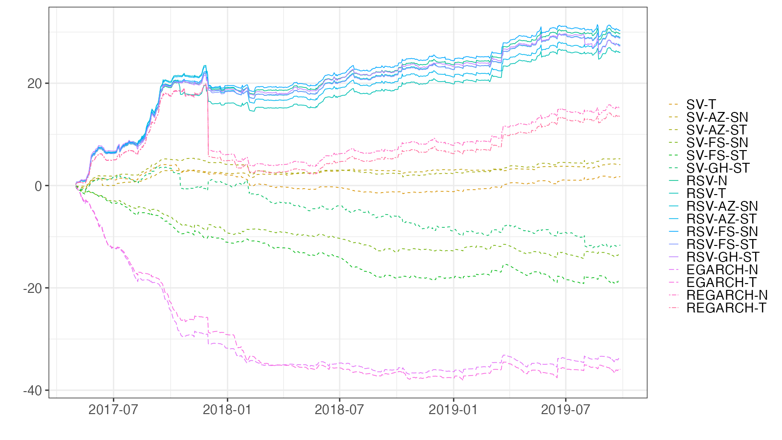
Figure 8: Cumulative loss differences (QLIKE) in comparison to the SV-N model for DJIA.

The prediction results for N225 mirror those obtained for DJIA, emphasizing that the incorporation of RV refines volatility forecasts. The details are provided in Appendix B.1.

4.3.2 VaR and ES forecasts

Figure 9 depicts the VaR and ES forecasts of the RSV-FS-ST and REGARCH-T models for DJIA. Notably, VaR violations (instances where actual returns drop below the VaR forecasts) manifest consistently across models. These violations are evident not only during turbulent phases like early 2018 and late 2019 but also during calmer periods. While the VaR and ES forecasts of other models exhibit similar trajectories with minor level variations, they are excluded here for conciseness.

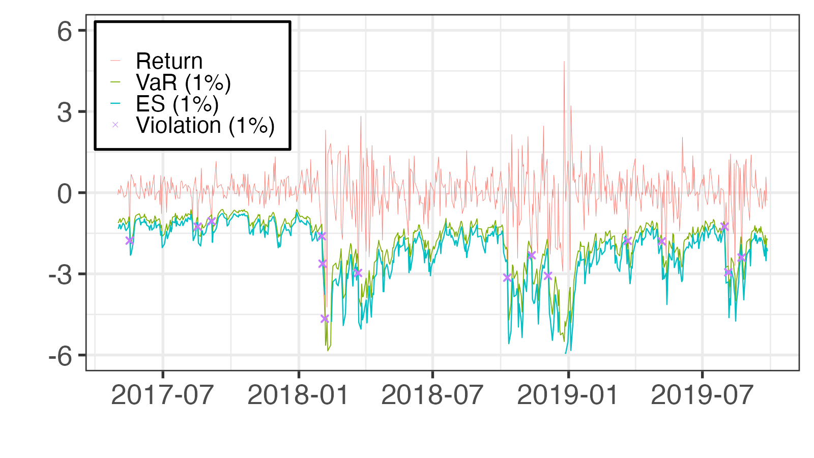
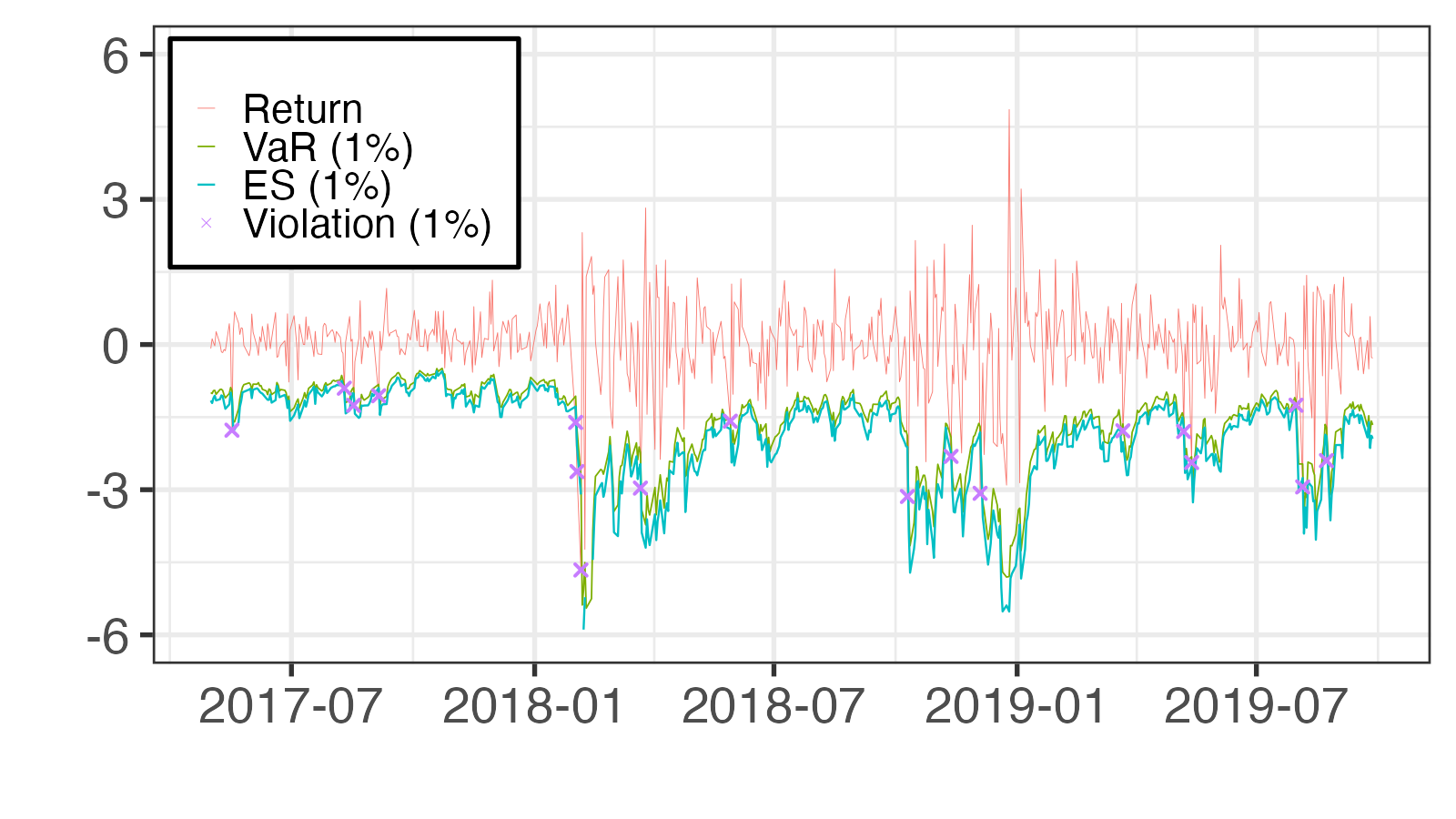
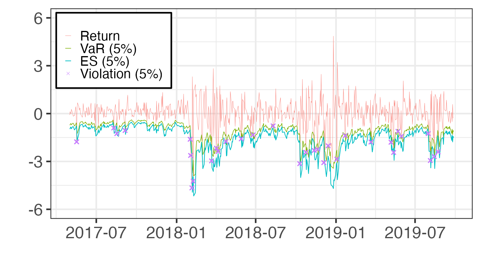
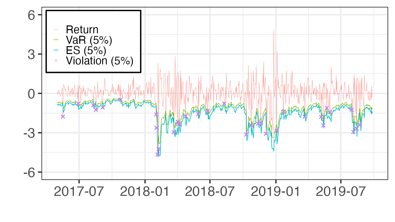
Figure 9: VaR and ES forecasts for DJIA: RSV-FS-ST model (left) vs. REGARCH-T model (right).

Table 5 reports the violation rates of the VaR forecasts, denoted as $\hat{\alpha}$, along with the average losses determined by the FZ0 loss function as described by Patton et al. (2019) in equation (59). The SV-GH-ST and EGARCH-T models yield violation rates nearest to the target rates of $\alpha=1\%$ and 5%, respectively. For the target rate $\alpha=1\%$, every model demonstrates violation rates above 1%, suggesting that actual returns surpass the VaR forecasts more frequently than anticipated. When $\alpha=5\%$, the violation rates gravitate closely around 5%. Conversely, the SV-AZ-SN and RSV-AZ-ST models display the minimal FZ0 loss for $\alpha=1\%$ and 5%, respectively, insinuating their superior performance in forecasting the return distribution’s tail. It is worth noting that, with the exception of the SV-GH-ST model for $\alpha=5\%$, all models fall within the 75% MCS for both $\alpha=1\%$ and 5%.

Table 5: Violation rates and FZ0 losses of VaR and ES forecasts for DJIA

	$\alpha=1\%$				$\alpha=5\%$
	$\hat{\alpha}$	FZ0	$p_{MCS}$		$\hat{\alpha}$	FZ0	$p_{MCS}$
SV-N	$2.32$	$1.0714$	$1.00^{**}$		$4.64$	$0.5965$	$0.76^{**}$
SV-T	$1.99$	$1.0483$	$1.00^{**}$		$4.31$	$0.5809$	$1.00^{**}$
SV-AZ-SN	$1.82$	$0.9698$	$1.00^{**}$		$4.31$	$0.5858$	$0.99^{**}$
SV-AZ-ST	$1.82$	$1.0180$	$1.00^{**}$		$4.31$	$0.5830$	$1.00^{**}$
SV-FS-SN	$1.49$	$0.9786$	$1.00^{**}$		$4.15$	$0.5947$	$0.90^{**}$
SV-FS-ST	$1.49$	$0.9899$	$1.00^{**}$		$4.15$	$0.5954$	$0.87^{**}$
SV-GH-ST	$1.33$	$1.1224$	$1.00^{**}$		$4.31$	$0.7012$	$0.12^{*\hskip 2.79996pt}$
RSV-N	$2.99$	$1.2445$	$0.45^{**}$		$5.64$	$0.5584$	$1.00^{**}$
RSV-T	$2.82$	$1.1419$	$0.98^{**}$		$5.80$	$0.5465$	$1.00^{**}$
RSV-AZ-SN	$2.32$	$1.1282$	$1.00^{**}$		$5.47$	$0.5414$	$1.00^{**}$
RSV-AZ-ST	$2.16$	$1.0780$	$1.00^{**}$		$5.14$	$0.5299$	$1.00^{**}$
RSV-FS-SN	$2.32$	$1.0490$	$1.00^{**}$		$5.64$	$0.5411$	$1.00^{**}$
RSV-FS-ST	$2.49$	$1.0958$	$1.00^{**}$		$5.31$	$0.5365$	$1.00^{**}$
RSV-GH-ST	$2.16$	$1.0689$	$1.00^{**}$		$5.64$	$0.5387$	$1.00^{**}$
EGARCH-N	$2.65$	$1.2928$	$0.39^{**}$		$4.81$	$0.6226$	$0.35^{**}$
EGARCH-T	$1.82$	$1.0797$	$1.00^{**}$		$4.98$	$0.5855$	$1.00^{**}$
REGARCH-N	$3.15$	$1.3273$	$0.30^{**}$		$5.47$	$0.5652$	$1.00^{**}$
REGARCH-T	$2.99$	$1.3202$	$0.32^{**}$		$5.47$	$0.5621$	$1.00^{**}$

Notes: $\hat{\alpha}$ represents violation rate (%). FZ0 denotes the average FZ0 loss. $p_{MCS}$ indicates the MCS $p$-value. ${}^{**},{}^{*}$ correspond to models within the 75% and 90% MCS, respectively.

Tables 6 and 7 present the GW test results for the FZ0 loss. The lower and upper triangular elements are interpreted as in Table 4. The test statistics of the unconditional GW tests from the lower triangular elements indicate that the SV-AZ-SN model significantly outperforms the SV-N model, while the RSV-N model is significantly inferior to the other RSV models at $\alpha=1\%$. Furthermore, the EGARCH-T model exhibits superior performance compared to the EGARCH-N model. The proportions of predicted losses from the conditional GW tests in the upper triangular elements echo these findings. These outcomes underscore the significance of accounting for heavy tails when forecasting return distributions. Additionally, it is observed that all RSV models, with the exception of RSV-N and RSV-GH-ST, perform significantly better than the REGARCH models at $\alpha=1\%$.

Table 6: Summary of GW tests on FZ0 loss of VaR and ES forecasts ($\alpha=1\%$) for DJIA

	SV-N	T	AZ-SN	AZ-ST	FS-SN	FS-ST	GH-ST	RSV-N	T	AZ-SN	AZ-ST	FS-SN	FS-ST	GH-ST	EG-N	T	REG-N	T
SV-N		$\hskip 3.49998pt\hskip 1.99997pt94^{\hskip 2.8pt}$	$\hskip 3.49998pt\hskip 1.99997pt99^{\hskip 2.8pt}$	$\hskip 3.49998pt\hskip 1.99997pt99^{\hskip 2.8pt}$	$\hskip 3.49998pt100^{\hskip 2.8pt}$	$\hskip 3.49998pt\hskip 1.99997pt99^{\hskip 2.8pt}$	$\hskip 3.49998pt\hskip 1.99997pt\hskip 1.99997pt6^{\hskip 2.8pt}$	$\hskip 3.49998pt\hskip 1.99997pt\hskip 1.99997pt1^{\hskip 2.8pt}$	$\hskip 3.49998pt\hskip 1.99997pt\hskip 1.99997pt2^{\hskip 2.8pt}$	$\hskip 3.49998pt\hskip 1.99997pt\hskip 1.99997pt8^{\hskip 2.8pt}$	$\hskip 3.49998pt\hskip 1.99997pt54^{\hskip 2.8pt}$	$\hskip 3.49998pt\hskip 1.99997pt99^{\hskip 2.8pt}$	$\hskip 3.49998pt\hskip 1.99997pt12^{\hskip 2.8pt}$	$\hskip 3.49998pt\hskip 1.99997pt67^{\hskip 2.8pt}$	$\hskip 3.49998pt\hskip 1.99997pt\hskip 1.99997pt1^{\hskip 2.8pt}$	$\hskip 3.49998pt\hskip 1.99997pt23^{\hskip 2.8pt}$	$\hskip 3.49998pt\hskip 1.99997pt\hskip 1.99997pt1^{\hskip 2.8pt}$	$\hskip 3.49998pt\hskip 1.99997pt\hskip 1.99997pt1^{\hskip 2.8pt}$
SV-T	$-0.4^{\hskip 2.8pt}$		$\hskip 3.49998pt\hskip 1.99997pt99^{*\hskip 1.39998pt}$	$\hskip 3.49998pt100^{\hskip 2.8pt}$	$\hskip 3.49998pt\hskip 1.99997pt35^{\hskip 2.8pt}$	$\hskip 3.49998pt100^{\hskip 2.8pt}$	$\hskip 3.49998pt\hskip 1.99997pt\hskip 1.99997pt7^{\hskip 2.8pt}$	$\hskip 3.49998pt\hskip 1.99997pt\hskip 1.99997pt0^{\hskip 2.8pt}$	$\hskip 3.49998pt\hskip 1.99997pt\hskip 1.99997pt0^{\hskip 2.8pt}$	$\hskip 3.49998pt\hskip 1.99997pt\hskip 1.99997pt0^{\hskip 2.8pt}$	$\hskip 3.49998pt\hskip 1.99997pt\hskip 1.99997pt1^{\hskip 2.8pt}$	$\hskip 3.49998pt\hskip 1.99997pt14^{\hskip 2.8pt}$	$\hskip 3.49998pt\hskip 1.99997pt\hskip 1.99997pt1^{\hskip 2.8pt}$	$\hskip 3.49998pt\hskip 1.99997pt\hskip 1.99997pt0^{\hskip 2.8pt}$	$\hskip 3.49998pt\hskip 1.99997pt\hskip 1.99997pt2^{*\hskip 1.39998pt}$	$\hskip 3.49998pt\hskip 1.99997pt\hskip 1.99997pt2^{\hskip 2.8pt}$	$\hskip 3.49998pt\hskip 1.99997pt\hskip 1.99997pt0^{\hskip 2.8pt}$	$\hskip 3.49998pt\hskip 1.99997pt\hskip 1.99997pt0^{\hskip 2.8pt}$
SV-AZ-SN	$-2.2^{*\hskip 1.39998pt}$	$-1.6^{\hskip 2.8pt}$		$\hskip 3.49998pt\hskip 1.99997pt\hskip 1.99997pt4^{\hskip 2.8pt}$	$\hskip 3.49998pt\hskip 1.99997pt\hskip 1.99997pt6^{\hskip 2.8pt}$	$\hskip 3.49998pt\hskip 1.99997pt\hskip 1.99997pt0^{\hskip 2.8pt}$	$\hskip 3.49998pt\hskip 1.99997pt\hskip 1.99997pt2^{\hskip 2.8pt}$	$\hskip 3.49998pt\hskip 1.99997pt\hskip 1.99997pt0^{\hskip 2.8pt}$	$\hskip 3.49998pt\hskip 1.99997pt\hskip 1.99997pt0^{\hskip 2.8pt}$	$\hskip 3.49998pt\hskip 1.99997pt\hskip 1.99997pt0^{\hskip 2.8pt}$	$\hskip 3.49998pt\hskip 1.99997pt\hskip 1.99997pt1^{\hskip 2.8pt}$	$\hskip 3.49998pt\hskip 1.99997pt\hskip 1.99997pt0^{\hskip 2.8pt}$	$\hskip 3.49998pt\hskip 1.99997pt\hskip 1.99997pt0^{\hskip 2.8pt}$	$\hskip 3.49998pt\hskip 1.99997pt\hskip 1.99997pt1^{\hskip 2.8pt}$	$\hskip 3.49998pt\hskip 1.99997pt\hskip 1.99997pt1^{\hskip 2.8pt}$	$\hskip 3.49998pt\hskip 1.99997pt\hskip 1.99997pt1^{\hskip 2.8pt}$	$\hskip 3.49998pt\hskip 1.99997pt\hskip 1.99997pt0^{\hskip 2.8pt}$	$\hskip 3.49998pt\hskip 1.99997pt\hskip 1.99997pt0^{\hskip 2.8pt}$
SV-AZ-ST	$-0.9^{\hskip 2.8pt}$	$-1.0^{\hskip 2.8pt}$	$\hskip 3.49998pt1.4^{\hskip 2.8pt}$		$\hskip 3.49998pt\hskip 1.99997pt47^{\hskip 2.8pt}$	$\hskip 3.49998pt\hskip 1.99997pt59^{\hskip 2.8pt}$	$\hskip 3.49998pt\hskip 1.99997pt\hskip 1.99997pt4^{\hskip 2.8pt}$	$\hskip 3.49998pt\hskip 1.99997pt\hskip 1.99997pt0^{\hskip 2.8pt}$	$\hskip 3.49998pt\hskip 1.99997pt\hskip 1.99997pt0^{\hskip 2.8pt}$	$\hskip 3.49998pt\hskip 1.99997pt\hskip 1.99997pt0^{\hskip 2.8pt}$	$\hskip 3.49998pt\hskip 1.99997pt\hskip 1.99997pt0^{\hskip 2.8pt}$	$\hskip 3.49998pt\hskip 1.99997pt\hskip 1.99997pt1^{\hskip 2.8pt}$	$\hskip 3.49998pt\hskip 1.99997pt\hskip 1.99997pt0^{\hskip 2.8pt}$	$\hskip 3.49998pt\hskip 1.99997pt\hskip 1.99997pt1^{\hskip 2.8pt}$	$\hskip 3.49998pt\hskip 1.99997pt\hskip 1.99997pt2^{*\hskip 1.39998pt}$	$\hskip 3.49998pt\hskip 1.99997pt\hskip 1.99997pt1^{\hskip 2.8pt}$	$\hskip 3.49998pt\hskip 1.99997pt\hskip 1.99997pt0^{\hskip 2.8pt}$	$\hskip 3.49998pt\hskip 1.99997pt\hskip 1.99997pt0^{\hskip 2.8pt}$
SV-FS-SN	$-1.5^{\hskip 2.8pt}$	$-0.8^{\hskip 2.8pt}$	$\hskip 3.49998pt0.2^{\hskip 2.8pt}$	$-0.6^{\hskip 2.8pt}$		$\hskip 3.49998pt\hskip 1.99997pt11^{\hskip 2.8pt}$	$\hskip 3.49998pt\hskip 1.99997pt\hskip 1.99997pt2^{\hskip 2.8pt}$	$\hskip 3.49998pt\hskip 1.99997pt\hskip 1.99997pt0^{\hskip 2.8pt}$	$\hskip 3.49998pt\hskip 1.99997pt\hskip 1.99997pt0^{\hskip 2.8pt}$	$\hskip 3.49998pt\hskip 1.99997pt\hskip 1.99997pt5^{\hskip 2.8pt}$	$\hskip 3.49998pt\hskip 1.99997pt16^{\hskip 2.8pt}$	$\hskip 3.49998pt\hskip 1.99997pt\hskip 1.99997pt0^{\hskip 2.8pt}$	$\hskip 3.49998pt\hskip 1.99997pt\hskip 1.99997pt4^{\hskip 2.8pt}$	$\hskip 3.49998pt\hskip 1.99997pt\hskip 1.99997pt0^{\hskip 2.8pt}$	$\hskip 3.49998pt\hskip 1.99997pt\hskip 1.99997pt0^{\hskip 2.8pt}$	$\hskip 3.49998pt\hskip 1.99997pt\hskip 1.99997pt0^{\hskip 2.8pt}$	$\hskip 3.49998pt\hskip 1.99997pt\hskip 1.99997pt0^{\hskip 2.8pt}$	$\hskip 3.49998pt\hskip 1.99997pt\hskip 1.99997pt0^{\hskip 2.8pt}$
SV-FS-ST	$-1.4^{\hskip 2.8pt}$	$-0.9^{\hskip 2.8pt}$	$\hskip 3.49998pt0.9^{\hskip 2.8pt}$	$-0.7^{\hskip 2.8pt}$	$\hskip 3.49998pt0.3^{\hskip 2.8pt}$		$\hskip 3.49998pt\hskip 1.99997pt\hskip 1.99997pt2^{\hskip 2.8pt}$	$\hskip 3.49998pt\hskip 1.99997pt\hskip 1.99997pt0^{\hskip 2.8pt}$	$\hskip 3.49998pt\hskip 1.99997pt\hskip 1.99997pt0^{\hskip 2.8pt}$	$\hskip 3.49998pt\hskip 1.99997pt\hskip 1.99997pt0^{\hskip 2.8pt}$	$\hskip 3.49998pt\hskip 1.99997pt\hskip 1.99997pt0^{\hskip 2.8pt}$	$\hskip 3.49998pt\hskip 1.99997pt\hskip 1.99997pt0^{\hskip 2.8pt}$	$\hskip 3.49998pt\hskip 1.99997pt\hskip 1.99997pt0^{\hskip 2.8pt}$	$\hskip 3.49998pt\hskip 1.99997pt\hskip 1.99997pt1^{\hskip 2.8pt}$	$\hskip 3.49998pt\hskip 1.99997pt\hskip 1.99997pt1^{\hskip 2.8pt}$	$\hskip 3.49998pt\hskip 1.99997pt\hskip 1.99997pt1^{\hskip 2.8pt}$	$\hskip 3.49998pt\hskip 1.99997pt\hskip 1.99997pt0^{\hskip 2.8pt}$	$\hskip 3.49998pt\hskip 1.99997pt\hskip 1.99997pt0^{\hskip 2.8pt}$
SV-GH-ST	$\hskip 3.49998pt0.5^{\hskip 2.8pt}$	$\hskip 3.49998pt0.8^{\hskip 2.8pt}$	$\hskip 3.49998pt2.0^{*\hskip 1.39998pt}$	$\hskip 3.49998pt1.5^{\hskip 2.8pt}$	$\hskip 3.49998pt1.5^{\hskip 2.8pt}$	$\hskip 3.49998pt1.9^{\hskip 2.8pt}$		$\hskip 3.49998pt\hskip 1.99997pt\hskip 1.99997pt2^{\hskip 2.8pt}$	$\hskip 3.49998pt\hskip 1.99997pt\hskip 1.99997pt2^{\hskip 2.8pt}$	$\hskip 3.49998pt\hskip 1.99997pt\hskip 1.99997pt4^{\hskip 2.8pt}$	$\hskip 3.49998pt\hskip 1.99997pt89^{\hskip 2.8pt}$	$\hskip 3.49998pt\hskip 1.99997pt96^{\hskip 2.8pt}$	$\hskip 3.49998pt\hskip 1.99997pt57^{\hskip 2.8pt}$	$\hskip 3.49998pt\hskip 1.99997pt92^{\hskip 2.8pt}$	$\hskip 3.49998pt\hskip 1.99997pt\hskip 1.99997pt2^{\hskip 2.8pt}$	$\hskip 3.49998pt\hskip 1.99997pt71^{\hskip 2.8pt}$	$\hskip 3.49998pt\hskip 1.99997pt\hskip 1.99997pt0^{\hskip 2.8pt}$	$\hskip 3.49998pt\hskip 1.99997pt\hskip 1.99997pt0^{\hskip 2.8pt}$
RSV-N	$\hskip 3.49998pt1.1^{\hskip 2.8pt}$	$\hskip 3.49998pt1.4^{\hskip 2.8pt}$	$\hskip 3.49998pt1.6^{\hskip 2.8pt}$	$\hskip 3.49998pt1.5^{\hskip 2.8pt}$	$\hskip 3.49998pt1.4^{\hskip 2.8pt}$	$\hskip 3.49998pt1.4^{\hskip 2.8pt}$	$\hskip 3.49998pt0.6^{\hskip 2.8pt}$		$\hskip 3.49998pt100^{*\hskip 1.39998pt}$	$\hskip 3.49998pt100^{*\hskip 1.39998pt}$	$\hskip 3.49998pt100^{\hskip 2.8pt}$	$\hskip 3.49998pt100^{*\hskip 1.39998pt}$	$\hskip 3.49998pt100^{*\hskip 1.39998pt}$	$\hskip 3.49998pt100^{\hskip 2.8pt}$	$\hskip 3.49998pt\hskip 1.99997pt\hskip 1.99997pt2^{\hskip 2.8pt}$	$\hskip 3.49998pt\hskip 1.99997pt99^{\hskip 2.8pt}$	$\hskip 3.49998pt\hskip 1.99997pt\hskip 1.99997pt1^{\hskip 2.8pt}$	$\hskip 3.49998pt\hskip 1.99997pt\hskip 1.99997pt1^{\hskip 2.8pt}$
RSV-T	$\hskip 3.49998pt0.6^{\hskip 2.8pt}$	$\hskip 3.49998pt0.9^{\hskip 2.8pt}$	$\hskip 3.49998pt1.3^{\hskip 2.8pt}$	$\hskip 3.49998pt1.0^{\hskip 2.8pt}$	$\hskip 3.49998pt1.1^{\hskip 2.8pt}$	$\hskip 3.49998pt1.0^{\hskip 2.8pt}$	$\hskip 3.49998pt0.1^{\hskip 2.8pt}$	$-2.4^{*\hskip 1.39998pt}$		$\hskip 3.49998pt\hskip 1.99997pt99^{\hskip 2.8pt}$	$\hskip 3.49998pt100^{**}$	$\hskip 3.49998pt100^{\hskip 2.8pt}$	$\hskip 3.49998pt100^{\hskip 2.8pt}$	$\hskip 3.49998pt\hskip 1.99997pt93^{\hskip 2.8pt}$	$\hskip 3.49998pt\hskip 1.99997pt\hskip 1.99997pt2^{\hskip 2.8pt}$	$\hskip 3.49998pt\hskip 1.99997pt98^{\hskip 2.8pt}$	$\hskip 3.49998pt\hskip 1.99997pt\hskip 1.99997pt0^{*\hskip 1.39998pt}$	$\hskip 3.49998pt\hskip 1.99997pt\hskip 1.99997pt0^{*\hskip 1.39998pt}$
RSV-AZ-SN	$\hskip 3.49998pt0.5^{\hskip 2.8pt}$	$\hskip 3.49998pt0.8^{\hskip 2.8pt}$	$\hskip 3.49998pt1.2^{\hskip 2.8pt}$	$\hskip 3.49998pt1.0^{\hskip 2.8pt}$	$\hskip 3.49998pt1.0^{\hskip 2.8pt}$	$\hskip 3.49998pt1.0^{\hskip 2.8pt}$	$\hskip 3.49998pt0.0^{\hskip 2.8pt}$	$-2.4^{*\hskip 1.39998pt}$	$-0.7^{\hskip 2.8pt}$		$\hskip 3.49998pt100^{\hskip 2.8pt}$	$\hskip 3.49998pt\hskip 1.99997pt97^{\hskip 2.8pt}$	$\hskip 3.49998pt\hskip 1.99997pt98^{\hskip 2.8pt}$	$\hskip 3.49998pt\hskip 1.99997pt81^{\hskip 2.8pt}$	$\hskip 3.49998pt\hskip 1.99997pt\hskip 1.99997pt2^{\hskip 2.8pt}$	$\hskip 3.49998pt\hskip 1.99997pt99^{\hskip 2.8pt}$	$\hskip 3.49998pt\hskip 1.99997pt\hskip 1.99997pt0^{*\hskip 1.39998pt}$	$\hskip 3.49998pt\hskip 1.99997pt\hskip 1.99997pt0^{*\hskip 1.39998pt}$
RSV-AZ-ST	$\hskip 3.49998pt0.1^{\hskip 2.8pt}$	$\hskip 3.49998pt0.3^{\hskip 2.8pt}$	$\hskip 3.49998pt1.0^{\hskip 2.8pt}$	$\hskip 3.49998pt0.6^{\hskip 2.8pt}$	$\hskip 3.49998pt0.8^{\hskip 2.8pt}$	$\hskip 3.49998pt0.7^{\hskip 2.8pt}$	$-0.3^{\hskip 2.8pt}$	$-2.3^{*\hskip 1.39998pt}$	$-1.8^{\hskip 2.8pt}$	$-1.7^{\hskip 2.8pt}$		$\hskip 3.49998pt\hskip 1.99997pt90^{\hskip 2.8pt}$	$\hskip 3.49998pt\hskip 1.99997pt\hskip 1.99997pt0^{\hskip 2.8pt}$	$\hskip 3.49998pt\hskip 1.99997pt67^{\hskip 2.8pt}$	$\hskip 3.49998pt\hskip 1.99997pt\hskip 1.99997pt2^{\hskip 2.8pt}$	$\hskip 3.49998pt\hskip 1.99997pt62^{\hskip 2.8pt}$	$\hskip 3.49998pt\hskip 1.99997pt\hskip 1.99997pt0^{*\hskip 1.39998pt}$	$\hskip 3.49998pt\hskip 1.99997pt\hskip 1.99997pt0^{*\hskip 1.39998pt}$
RSV-FS-SN	$-0.2^{\hskip 2.8pt}$	$\hskip 3.49998pt0.0^{\hskip 2.8pt}$	$\hskip 3.49998pt0.9^{\hskip 2.8pt}$	$\hskip 3.49998pt0.3^{\hskip 2.8pt}$	$\hskip 3.49998pt0.7^{\hskip 2.8pt}$	$\hskip 3.49998pt0.6^{\hskip 2.8pt}$	$-0.6^{\hskip 2.8pt}$	$-2.1^{*\hskip 1.39998pt}$	$-1.5^{\hskip 2.8pt}$	$-1.2^{\hskip 2.8pt}$	$-0.6^{\hskip 2.8pt}$		$\hskip 3.49998pt\hskip 1.99997pt\hskip 1.99997pt1^{\hskip 2.8pt}$	$\hskip 3.49998pt\hskip 1.99997pt\hskip 1.99997pt1^{\hskip 2.8pt}$	$\hskip 3.49998pt\hskip 1.99997pt\hskip 1.99997pt2^{\hskip 2.8pt}$	$\hskip 3.49998pt\hskip 1.99997pt\hskip 1.99997pt6^{\hskip 2.8pt}$	$\hskip 3.49998pt\hskip 1.99997pt\hskip 1.99997pt0^{*\hskip 1.39998pt}$	$\hskip 3.49998pt\hskip 1.99997pt\hskip 1.99997pt0^{*\hskip 1.39998pt}$
RSV-FS-ST	$\hskip 3.49998pt0.2^{\hskip 2.8pt}$	$\hskip 3.49998pt0.5^{\hskip 2.8pt}$	$\hskip 3.49998pt1.1^{\hskip 2.8pt}$	$\hskip 3.49998pt0.8^{\hskip 2.8pt}$	$\hskip 3.49998pt0.9^{\hskip 2.8pt}$	$\hskip 3.49998pt0.8^{\hskip 2.8pt}$	$-0.2^{\hskip 2.8pt}$	$-2.4^{*\hskip 1.39998pt}$	$-1.7^{\hskip 2.8pt}$	$-1.2^{\hskip 2.8pt}$	$\hskip 3.49998pt0.9^{\hskip 2.8pt}$	$\hskip 3.49998pt1.1^{\hskip 2.8pt}$		$\hskip 3.49998pt\hskip 1.99997pt83^{\hskip 2.8pt}$	$\hskip 3.49998pt\hskip 1.99997pt\hskip 1.99997pt2^{\hskip 2.8pt}$	$\hskip 3.49998pt\hskip 1.99997pt98^{\hskip 2.8pt}$	$\hskip 3.49998pt\hskip 1.99997pt\hskip 1.99997pt0^{*\hskip 1.39998pt}$	$\hskip 3.49998pt\hskip 1.99997pt\hskip 1.99997pt0^{*\hskip 1.39998pt}$
RSV-GH-ST	$0.0^{\hskip 2.8pt}$	$\hskip 3.49998pt0.2^{\hskip 2.8pt}$	$\hskip 3.49998pt1.0^{\hskip 2.8pt}$	$\hskip 3.49998pt0.5^{\hskip 2.8pt}$	$\hskip 3.49998pt0.8^{\hskip 2.8pt}$	$\hskip 3.49998pt0.7^{\hskip 2.8pt}$	$-0.4^{\hskip 2.8pt}$	$-1.7^{\hskip 2.8pt}$	$-1.0^{\hskip 2.8pt}$	$-0.7^{\hskip 2.8pt}$	$-0.1^{\hskip 2.8pt}$	$\hskip 3.49998pt0.5^{\hskip 2.8pt}$	$-0.4^{\hskip 2.8pt}$		$\hskip 3.49998pt\hskip 1.99997pt\hskip 1.99997pt1^{\hskip 2.8pt}$	$\hskip 3.49998pt\hskip 1.99997pt36^{\hskip 2.8pt}$	$\hskip 3.49998pt\hskip 1.99997pt\hskip 1.99997pt0^{\hskip 2.8pt}$	$\hskip 3.49998pt\hskip 1.99997pt\hskip 1.99997pt0^{\hskip 2.8pt}$
EGARCH-N	$\hskip 3.49998pt1.5^{\hskip 2.8pt}$	$\hskip 3.49998pt1.8^{\hskip 2.8pt}$	$\hskip 3.49998pt1.9^{\hskip 2.8pt}$	$\hskip 3.49998pt1.8^{\hskip 2.8pt}$	$\hskip 3.49998pt1.6^{\hskip 2.8pt}$	$\hskip 3.49998pt1.7^{\hskip 2.8pt}$	$\hskip 3.49998pt0.9^{\hskip 2.8pt}$	$\hskip 3.49998pt0.3^{\hskip 2.8pt}$	$\hskip 3.49998pt1.0^{\hskip 2.8pt}$	$\hskip 3.49998pt1.1^{\hskip 2.8pt}$	$\hskip 3.49998pt1.3^{\hskip 2.8pt}$	$\hskip 3.49998pt1.5^{\hskip 2.8pt}$	$\hskip 3.49998pt1.3^{\hskip 2.8pt}$	$\hskip 3.49998pt1.2^{\hskip 2.8pt}$		$\hskip 3.49998pt100^{\hskip 2.8pt}$	$\hskip 3.49998pt\hskip 1.99997pt\hskip 1.99997pt1^{\hskip 2.8pt}$	$\hskip 3.49998pt\hskip 1.99997pt\hskip 1.99997pt1^{\hskip 2.8pt}$
EGARCH-T	$\hskip 3.49998pt0.1^{\hskip 2.8pt}$	$\hskip 3.49998pt0.4^{\hskip 2.8pt}$	$\hskip 3.49998pt1.2^{\hskip 2.8pt}$	$\hskip 3.49998pt0.7^{\hskip 2.8pt}$	$\hskip 3.49998pt0.9^{\hskip 2.8pt}$	$\hskip 3.49998pt0.9^{\hskip 2.8pt}$	$-0.3^{\hskip 2.8pt}$	$-1.0^{\hskip 2.8pt}$	$-0.4^{\hskip 2.8pt}$	$-0.4^{\hskip 2.8pt}$	$\hskip 3.49998pt0.0^{\hskip 2.8pt}$	$\hskip 3.49998pt0.3^{\hskip 2.8pt}$	$-0.1^{\hskip 2.8pt}$	$\hskip 3.49998pt0.1^{\hskip 2.8pt}$	$-2.1^{*\hskip 1.39998pt}$		$\hskip 3.49998pt\hskip 1.99997pt\hskip 1.99997pt0^{\hskip 2.8pt}$	$\hskip 3.49998pt\hskip 1.99997pt\hskip 1.99997pt0^{\hskip 2.8pt}$
REGARCH-N	$\hskip 3.49998pt1.4^{\hskip 2.8pt}$	$\hskip 3.49998pt1.7^{\hskip 2.8pt}$	$\hskip 3.49998pt1.8^{\hskip 2.8pt}$	$\hskip 3.49998pt1.7^{\hskip 2.8pt}$	$\hskip 3.49998pt1.5^{\hskip 2.8pt}$	$\hskip 3.49998pt1.6^{\hskip 2.8pt}$	$\hskip 3.49998pt0.9^{\hskip 2.8pt}$	$\hskip 3.49998pt1.3^{\hskip 2.8pt}$	$\hskip 3.49998pt2.0^{*\hskip 1.39998pt}$	$\hskip 3.49998pt2.2^{*\hskip 1.39998pt}$	$\hskip 3.49998pt2.2^{*\hskip 1.39998pt}$	$\hskip 3.49998pt2.0^{\hskip 2.8pt}$	$\hskip 3.49998pt2.1^{*\hskip 1.39998pt}$	$\hskip 3.49998pt1.7^{\hskip 2.8pt}$	$\hskip 3.49998pt0.2^{\hskip 2.8pt}$	$\hskip 3.49998pt1.4^{\hskip 2.8pt}$		$\hskip 3.49998pt\hskip 1.99997pt98^{\hskip 2.8pt}$
REGARCH-T	$\hskip 3.49998pt1.4^{\hskip 2.8pt}$	$\hskip 3.49998pt1.6^{\hskip 2.8pt}$	$\hskip 3.49998pt1.7^{\hskip 2.8pt}$	$\hskip 3.49998pt1.6^{\hskip 2.8pt}$	$\hskip 3.49998pt1.5^{\hskip 2.8pt}$	$\hskip 3.49998pt1.5^{\hskip 2.8pt}$	$\hskip 3.49998pt0.9^{\hskip 2.8pt}$	$\hskip 3.49998pt1.2^{\hskip 2.8pt}$	$\hskip 3.49998pt2.0^{*\hskip 1.39998pt}$	$\hskip 3.49998pt2.1^{*\hskip 1.39998pt}$	$\hskip 3.49998pt2.2^{*\hskip 1.39998pt}$	$\hskip 3.49998pt1.9^{\hskip 2.8pt}$	$\hskip 3.49998pt2.1^{*\hskip 1.39998pt}$	$\hskip 3.49998pt1.6^{\hskip 2.8pt}$	$\hskip 3.49998pt0.2^{\hskip 2.8pt}$	$\hskip 3.49998pt1.4^{\hskip 2.8pt}$	$-1.8^{\hskip 2.8pt}$

Note: Refer to Table 4 for additional details.

Table 7: Summary of GW tests on FZ0 loss of VaR and ES forecasts ($\alpha=5\%$) for DJIA

	SV-N	T	AZ-SN	AZ-ST	FS-SN	FS-ST	GH-ST	RSV-N	T	AZ-SN	AZ-ST	FS-SN	FS-ST	GH-ST	EG-N	T	REG-N	T
SV-N		$\hskip 3.49998pt\hskip 1.99997pt96^{\hskip 2.8pt}$	$\hskip 3.49998pt\hskip 1.99997pt99^{\hskip 2.8pt}$	$\hskip 3.49998pt\hskip 1.99997pt98^{\hskip 2.8pt}$	$\hskip 3.49998pt\hskip 1.99997pt95^{\hskip 2.8pt}$	$\hskip 3.49998pt\hskip 1.99997pt92^{\hskip 2.8pt}$	$\hskip 3.49998pt\hskip 1.99997pt\hskip 1.99997pt1^{\hskip 2.8pt}$	$\hskip 3.49998pt\hskip 1.99997pt96^{\hskip 2.8pt}$	$\hskip 3.49998pt\hskip 1.99997pt97^{\hskip 2.8pt}$	$\hskip 3.49998pt\hskip 1.99997pt98^{\hskip 2.8pt}$	$\hskip 3.49998pt\hskip 1.99997pt98^{\hskip 2.8pt}$	$\hskip 3.49998pt\hskip 1.99997pt99^{\hskip 2.8pt}$	$\hskip 3.49998pt\hskip 1.99997pt98^{\hskip 2.8pt}$	$\hskip 3.49998pt100^{\hskip 2.8pt}$	$\hskip 3.49998pt\hskip 1.99997pt\hskip 1.99997pt2^{\hskip 2.8pt}$	$\hskip 3.49998pt\hskip 1.99997pt80^{\hskip 2.8pt}$	$\hskip 3.49998pt\hskip 1.99997pt95^{\hskip 2.8pt}$	$\hskip 3.49998pt\hskip 1.99997pt96^{\hskip 2.8pt}$
SV-T	$-0.6^{\hskip 2.8pt}$		$\hskip 3.49998pt\hskip 1.99997pt\hskip 1.99997pt7^{\hskip 2.8pt}$	$\hskip 3.49998pt\hskip 1.99997pt\hskip 1.99997pt5^{\hskip 2.8pt}$	$\hskip 3.49998pt\hskip 1.99997pt\hskip 1.99997pt7^{\hskip 2.8pt}$	$\hskip 3.49998pt\hskip 1.99997pt\hskip 1.99997pt5^{\hskip 2.8pt}$	$\hskip 3.49998pt\hskip 1.99997pt\hskip 1.99997pt0^{\hskip 2.8pt}$	$\hskip 3.49998pt\hskip 1.99997pt99^{\hskip 2.8pt}$	$\hskip 3.49998pt\hskip 1.99997pt99^{\hskip 2.8pt}$	$\hskip 3.49998pt\hskip 1.99997pt99^{\hskip 2.8pt}$	$\hskip 3.49998pt\hskip 1.99997pt99^{\hskip 2.8pt}$	$\hskip 3.49998pt\hskip 1.99997pt99^{\hskip 2.8pt}$	$\hskip 3.49998pt\hskip 1.99997pt99^{\hskip 2.8pt}$	$\hskip 3.49998pt\hskip 1.99997pt99^{\hskip 2.8pt}$	$\hskip 3.49998pt\hskip 1.99997pt\hskip 1.99997pt2^{\hskip 2.8pt}$	$\hskip 3.49998pt\hskip 1.99997pt25^{\hskip 2.8pt}$	$\hskip 3.49998pt\hskip 1.99997pt98^{\hskip 2.8pt}$	$\hskip 3.49998pt\hskip 1.99997pt98^{\hskip 2.8pt}$
SV-AZ-SN	$-0.8^{\hskip 2.8pt}$	$\hskip 3.49998pt0.2^{\hskip 2.8pt}$		$\hskip 3.49998pt\hskip 1.99997pt86^{\hskip 2.8pt}$	$\hskip 3.49998pt\hskip 1.99997pt\hskip 1.99997pt4^{\hskip 2.8pt}$	$\hskip 3.49998pt\hskip 1.99997pt\hskip 1.99997pt0^{\hskip 2.8pt}$	$\hskip 3.49998pt\hskip 1.99997pt\hskip 1.99997pt0^{\hskip 2.8pt}$	$\hskip 3.49998pt\hskip 1.99997pt97^{\hskip 2.8pt}$	$\hskip 3.49998pt\hskip 1.99997pt98^{\hskip 2.8pt}$	$\hskip 3.49998pt\hskip 1.99997pt98^{\hskip 2.8pt}$	$\hskip 3.49998pt\hskip 1.99997pt98^{\hskip 2.8pt}$	$\hskip 3.49998pt100^{\hskip 2.8pt}$	$\hskip 3.49998pt\hskip 1.99997pt99^{\hskip 2.8pt}$	$\hskip 3.49998pt\hskip 1.99997pt99^{\hskip 2.8pt}$	$\hskip 3.49998pt\hskip 1.99997pt\hskip 1.99997pt2^{\hskip 2.8pt}$	$\hskip 3.49998pt\hskip 1.99997pt38^{\hskip 2.8pt}$	$\hskip 3.49998pt\hskip 1.99997pt96^{\hskip 2.8pt}$	$\hskip 3.49998pt\hskip 1.99997pt96^{\hskip 2.8pt}$
SV-AZ-ST	$-0.6^{\hskip 2.8pt}$	$\hskip 3.49998pt0.2^{\hskip 2.8pt}$	$-0.2^{\hskip 2.8pt}$		$\hskip 3.49998pt\hskip 1.99997pt\hskip 1.99997pt8^{\hskip 2.8pt}$	$\hskip 3.49998pt\hskip 1.99997pt\hskip 1.99997pt4^{\hskip 2.8pt}$	$\hskip 3.49998pt\hskip 1.99997pt\hskip 1.99997pt0^{\hskip 2.8pt}$	$\hskip 3.49998pt100^{\hskip 2.8pt}$	$\hskip 3.49998pt100^{\hskip 2.8pt}$	$\hskip 3.49998pt100^{\hskip 2.8pt}$	$\hskip 3.49998pt100^{\hskip 2.8pt}$	$\hskip 3.49998pt100^{\hskip 2.8pt}$	$\hskip 3.49998pt100^{\hskip 2.8pt}$	$\hskip 3.49998pt\hskip 1.99997pt99^{\hskip 2.8pt}$	$\hskip 3.49998pt\hskip 1.99997pt\hskip 1.99997pt3^{\hskip 2.8pt}$	$\hskip 3.49998pt\hskip 1.99997pt32^{\hskip 2.8pt}$	$\hskip 3.49998pt\hskip 1.99997pt97^{\hskip 2.8pt}$	$\hskip 3.49998pt\hskip 1.99997pt97^{\hskip 2.8pt}$
SV-FS-SN	$-0.1^{\hskip 2.8pt}$	$\hskip 3.49998pt0.5^{\hskip 2.8pt}$	$\hskip 3.49998pt0.8^{\hskip 2.8pt}$	$\hskip 3.49998pt0.5^{\hskip 2.8pt}$		$\hskip 3.49998pt\hskip 1.99997pt34^{\hskip 2.8pt}$	$\hskip 3.49998pt\hskip 1.99997pt\hskip 1.99997pt1^{\hskip 2.8pt}$	$\hskip 3.49998pt\hskip 1.99997pt96^{\hskip 2.8pt}$	$\hskip 3.49998pt\hskip 1.99997pt96^{\hskip 2.8pt}$	$\hskip 3.49998pt\hskip 1.99997pt97^{\hskip 2.8pt}$	$\hskip 3.49998pt\hskip 1.99997pt98^{\hskip 2.8pt}$	$\hskip 3.49998pt\hskip 1.99997pt98^{\hskip 2.8pt}$	$\hskip 3.49998pt\hskip 1.99997pt98^{\hskip 2.8pt}$	$\hskip 3.49998pt100^{\hskip 2.8pt}$	$\hskip 3.49998pt\hskip 1.99997pt\hskip 1.99997pt0^{\hskip 2.8pt}$	$\hskip 3.49998pt\hskip 1.99997pt63^{\hskip 2.8pt}$	$\hskip 3.49998pt\hskip 1.99997pt95^{\hskip 2.8pt}$	$\hskip 3.49998pt\hskip 1.99997pt96^{\hskip 2.8pt}$
SV-FS-ST	$-0.1^{\hskip 2.8pt}$	$\hskip 3.49998pt0.6^{\hskip 2.8pt}$	$\hskip 3.49998pt0.9^{\hskip 2.8pt}$	$\hskip 3.49998pt0.7^{\hskip 2.8pt}$	$\hskip 3.49998pt0.1^{\hskip 2.8pt}$		$\hskip 3.49998pt\hskip 1.99997pt\hskip 1.99997pt0^{\hskip 2.8pt}$	$\hskip 3.49998pt\hskip 1.99997pt97^{\hskip 2.8pt}$	$\hskip 3.49998pt\hskip 1.99997pt98^{\hskip 2.8pt}$	$\hskip 3.49998pt\hskip 1.99997pt98^{\hskip 2.8pt}$	$\hskip 3.49998pt\hskip 1.99997pt98^{\hskip 2.8pt}$	$\hskip 3.49998pt100^{\hskip 2.8pt}$	$\hskip 3.49998pt100^{\hskip 2.8pt}$	$\hskip 3.49998pt\hskip 1.99997pt99^{\hskip 2.8pt}$	$\hskip 3.49998pt\hskip 1.99997pt\hskip 1.99997pt3^{\hskip 2.8pt}$	$\hskip 3.49998pt\hskip 1.99997pt53^{\hskip 2.8pt}$	$\hskip 3.49998pt\hskip 1.99997pt96^{\hskip 2.8pt}$	$\hskip 3.49998pt\hskip 1.99997pt96^{\hskip 2.8pt}$
SV-GH-ST	$\hskip 3.49998pt1.7^{\hskip 2.8pt}$	$\hskip 3.49998pt2.0^{*\hskip 1.39998pt}$	$\hskip 3.49998pt2.0^{*\hskip 1.39998pt}$	$\hskip 3.49998pt2.0^{*\hskip 1.39998pt}$	$\hskip 3.49998pt1.7^{\hskip 2.8pt}$	$\hskip 3.49998pt1.8^{\hskip 2.8pt}$		$\hskip 3.49998pt100^{\hskip 2.8pt}$	$\hskip 3.49998pt100^{\hskip 2.8pt}$	$\hskip 3.49998pt100^{*\hskip 1.39998pt}$	$\hskip 3.49998pt100^{*\hskip 1.39998pt}$	$\hskip 3.49998pt100^{*\hskip 1.39998pt}$	$\hskip 3.49998pt100^{*\hskip 1.39998pt}$	$\hskip 3.49998pt100^{\hskip 2.8pt}$	$\hskip 3.49998pt\hskip 1.99997pt98^{\hskip 2.8pt}$	$\hskip 3.49998pt\hskip 1.99997pt98^{\hskip 2.8pt}$	$\hskip 3.49998pt100^{\hskip 2.8pt}$	$\hskip 3.49998pt100^{\hskip 2.8pt}$
RSV-N	$-1.0^{\hskip 2.8pt}$	$-0.6^{\hskip 2.8pt}$	$-0.7^{\hskip 2.8pt}$	$-0.6^{\hskip 2.8pt}$	$-0.8^{\hskip 2.8pt}$	$-0.8^{\hskip 2.8pt}$	$-2.1^{*\hskip 1.39998pt}$		$\hskip 3.49998pt100^{\hskip 2.8pt}$	$\hskip 3.49998pt\hskip 1.99997pt97^{\hskip 2.8pt}$	$\hskip 3.49998pt\hskip 1.99997pt97^{\hskip 2.8pt}$	$\hskip 3.49998pt\hskip 1.99997pt99^{\hskip 2.8pt}$	$\hskip 3.49998pt100^{\hskip 2.8pt}$	$\hskip 3.49998pt\hskip 1.99997pt99^{\hskip 2.8pt}$	$\hskip 3.49998pt\hskip 1.99997pt\hskip 1.99997pt1^{\hskip 2.8pt}$	$\hskip 3.49998pt\hskip 1.99997pt\hskip 1.99997pt1^{\hskip 2.8pt}$	$\hskip 3.49998pt\hskip 1.99997pt\hskip 1.99997pt8^{\hskip 2.8pt}$	$\hskip 3.49998pt\hskip 1.99997pt11^{\hskip 2.8pt}$
RSV-T	$-1.3^{\hskip 2.8pt}$	$-1.0^{\hskip 2.8pt}$	$-1.0^{\hskip 2.8pt}$	$-1.0^{\hskip 2.8pt}$	$-1.1^{\hskip 2.8pt}$	$-1.1^{\hskip 2.8pt}$	$-2.3^{*\hskip 1.39998pt}$	$-1.8^{\hskip 2.8pt}$		$\hskip 3.49998pt100^{*\hskip 1.39998pt}$	$\hskip 3.49998pt100^{\hskip 2.8pt}$	$\hskip 3.49998pt\hskip 1.99997pt58^{\hskip 2.8pt}$	$\hskip 3.49998pt\hskip 1.99997pt86^{\hskip 2.8pt}$	$\hskip 3.49998pt\hskip 1.99997pt81^{\hskip 2.8pt}$	$\hskip 3.49998pt\hskip 1.99997pt\hskip 1.99997pt1^{\hskip 2.8pt}$	$\hskip 3.49998pt\hskip 1.99997pt\hskip 1.99997pt1^{\hskip 2.8pt}$	$\hskip 3.49998pt\hskip 1.99997pt\hskip 1.99997pt4^{\hskip 2.8pt}$	$\hskip 3.49998pt\hskip 1.99997pt\hskip 1.99997pt5^{\hskip 2.8pt}$
RSV-AZ-SN	$-1.5^{\hskip 2.8pt}$	$-1.3^{\hskip 2.8pt}$	$-1.2^{\hskip 2.8pt}$	$-1.3^{\hskip 2.8pt}$	$-1.4^{\hskip 2.8pt}$	$-1.4^{\hskip 2.8pt}$	$-2.4^{*\hskip 1.39998pt}$	$-1.5^{\hskip 2.8pt}$	$-0.7^{\hskip 2.8pt}$		$\hskip 3.49998pt100^{\hskip 2.8pt}$	$\hskip 3.49998pt\hskip 1.99997pt74^{\hskip 2.8pt}$	$\hskip 3.49998pt\hskip 1.99997pt81^{\hskip 2.8pt}$	$\hskip 3.49998pt\hskip 1.99997pt74^{\hskip 2.8pt}$	$\hskip 3.49998pt\hskip 1.99997pt\hskip 1.99997pt2^{\hskip 2.8pt}$	$\hskip 3.49998pt\hskip 1.99997pt\hskip 1.99997pt1^{\hskip 2.8pt}$	$\hskip 3.49998pt\hskip 1.99997pt\hskip 1.99997pt2^{\hskip 2.8pt}$	$\hskip 3.49998pt\hskip 1.99997pt\hskip 1.99997pt3^{\hskip 2.8pt}$
RSV-AZ-ST	$-1.9^{\hskip 2.8pt}$	$-1.6^{\hskip 2.8pt}$	$-1.6^{\hskip 2.8pt}$	$-1.7^{\hskip 2.8pt}$	$-1.7^{\hskip 2.8pt}$	$-1.7^{\hskip 2.8pt}$	$-2.6^{**}$	$-1.9^{\hskip 2.8pt}$	$-1.6^{\hskip 2.8pt}$	$-2.3^{*\hskip 1.39998pt}$		$\hskip 3.49998pt\hskip 1.99997pt\hskip 1.99997pt1^{\hskip 2.8pt}$	$\hskip 3.49998pt\hskip 1.99997pt12^{\hskip 2.8pt}$	$\hskip 3.49998pt\hskip 1.99997pt\hskip 1.99997pt2^{\hskip 2.8pt}$	$\hskip 3.49998pt\hskip 1.99997pt\hskip 1.99997pt2^{\hskip 2.8pt}$	$\hskip 3.49998pt\hskip 1.99997pt\hskip 1.99997pt2^{\hskip 2.8pt}$	$\hskip 3.49998pt\hskip 1.99997pt\hskip 1.99997pt0^{\hskip 2.8pt}$	$\hskip 3.49998pt\hskip 1.99997pt\hskip 1.99997pt1^{\hskip 2.8pt}$
RSV-FS-SN	$-1.7^{\hskip 2.8pt}$	$-1.2^{\hskip 2.8pt}$	$-1.3^{\hskip 2.8pt}$	$-1.3^{\hskip 2.8pt}$	$-1.5^{\hskip 2.8pt}$	$-1.4^{\hskip 2.8pt}$	$-2.4^{*\hskip 1.39998pt}$	$-1.5^{\hskip 2.8pt}$	$-0.5^{\hskip 2.8pt}$	$0.0^{\hskip 2.8pt}$	$\hskip 3.49998pt1.1^{\hskip 2.8pt}$		$\hskip 3.49998pt100^{\hskip 2.8pt}$	$\hskip 3.49998pt\hskip 1.99997pt89^{\hskip 2.8pt}$	$\hskip 3.49998pt\hskip 1.99997pt\hskip 1.99997pt1^{\hskip 2.8pt}$	$\hskip 3.49998pt\hskip 1.99997pt\hskip 1.99997pt2^{\hskip 2.8pt}$	$\hskip 3.49998pt\hskip 1.99997pt\hskip 1.99997pt8^{\hskip 2.8pt}$	$\hskip 3.49998pt\hskip 1.99997pt\hskip 1.99997pt9^{\hskip 2.8pt}$
RSV-FS-ST	$-1.8^{\hskip 2.8pt}$	$-1.4^{\hskip 2.8pt}$	$-1.5^{\hskip 2.8pt}$	$-1.5^{\hskip 2.8pt}$	$-1.6^{\hskip 2.8pt}$	$-1.6^{\hskip 2.8pt}$	$-2.5^{*\hskip 1.39998pt}$	$-1.8^{\hskip 2.8pt}$	$-1.1^{\hskip 2.8pt}$	$-0.7^{\hskip 2.8pt}$	$\hskip 3.49998pt0.8^{\hskip 2.8pt}$	$-0.8^{\hskip 2.8pt}$		$\hskip 3.49998pt\hskip 1.99997pt12^{\hskip 2.8pt}$	$\hskip 3.49998pt\hskip 1.99997pt\hskip 1.99997pt2^{\hskip 2.8pt}$	$\hskip 3.49998pt\hskip 1.99997pt\hskip 1.99997pt2^{\hskip 2.8pt}$	$\hskip 3.49998pt\hskip 1.99997pt\hskip 1.99997pt5^{\hskip 2.8pt}$	$\hskip 3.49998pt\hskip 1.99997pt\hskip 1.99997pt7^{\hskip 2.8pt}$
RSV-GH-ST	$-1.7^{\hskip 2.8pt}$	$-1.2^{\hskip 2.8pt}$	$-1.4^{\hskip 2.8pt}$	$-1.3^{\hskip 2.8pt}$	$-1.5^{\hskip 2.8pt}$	$-1.5^{\hskip 2.8pt}$	$-2.4^{*\hskip 1.39998pt}$	$-1.0^{\hskip 2.8pt}$	$-0.4^{\hskip 2.8pt}$	$-0.2^{\hskip 2.8pt}$	$\hskip 3.49998pt0.5^{\hskip 2.8pt}$	$-0.2^{\hskip 2.8pt}$	$\hskip 3.49998pt0.1^{\hskip 2.8pt}$		$\hskip 3.49998pt\hskip 1.99997pt\hskip 1.99997pt2^{\hskip 2.8pt}$	$\hskip 3.49998pt\hskip 1.99997pt\hskip 1.99997pt4^{\hskip 2.8pt}$	$\hskip 3.49998pt\hskip 1.99997pt\hskip 1.99997pt9^{\hskip 2.8pt}$	$\hskip 3.49998pt\hskip 1.99997pt10^{\hskip 2.8pt}$
EGARCH-N	$\hskip 3.49998pt0.8^{\hskip 2.8pt}$	$\hskip 3.49998pt1.5^{\hskip 2.8pt}$	$\hskip 3.49998pt1.1^{\hskip 2.8pt}$	$\hskip 3.49998pt1.3^{\hskip 2.8pt}$	$\hskip 3.49998pt0.8^{\hskip 2.8pt}$	$\hskip 3.49998pt0.8^{\hskip 2.8pt}$	$-1.1^{\hskip 2.8pt}$	$\hskip 3.49998pt1.4^{\hskip 2.8pt}$	$\hskip 3.49998pt1.7^{\hskip 2.8pt}$	$\hskip 3.49998pt1.9^{\hskip 2.8pt}$	$\hskip 3.49998pt2.1^{*\hskip 1.39998pt}$	$\hskip 3.49998pt1.9^{\hskip 2.8pt}$	$\hskip 3.49998pt2.0^{*\hskip 1.39998pt}$	$\hskip 3.49998pt1.8^{\hskip 2.8pt}$		$\hskip 3.49998pt\hskip 1.99997pt99^{*\hskip 1.39998pt}$	$\hskip 3.49998pt\hskip 1.99997pt99^{\hskip 2.8pt}$	$\hskip 3.49998pt\hskip 1.99997pt99^{\hskip 2.8pt}$
EGARCH-T	$-0.4^{\hskip 2.8pt}$	$\hskip 3.49998pt0.2^{\hskip 2.8pt}$	$0.0^{\hskip 2.8pt}$	$\hskip 3.49998pt0.1^{\hskip 2.8pt}$	$-0.4^{\hskip 2.8pt}$	$-0.4^{\hskip 2.8pt}$	$-1.7^{\hskip 2.8pt}$	$\hskip 3.49998pt0.6^{\hskip 2.8pt}$	$\hskip 3.49998pt0.8^{\hskip 2.8pt}$	$\hskip 3.49998pt1.0^{\hskip 2.8pt}$	$\hskip 3.49998pt1.2^{\hskip 2.8pt}$	$\hskip 3.49998pt1.0^{\hskip 2.8pt}$	$\hskip 3.49998pt1.1^{\hskip 2.8pt}$	$\hskip 3.49998pt1.0^{\hskip 2.8pt}$	$-2.3^{*\hskip 1.39998pt}$		$\hskip 3.49998pt\hskip 1.99997pt99^{\hskip 2.8pt}$	$\hskip 3.49998pt100^{\hskip 2.8pt}$
REGARCH-N	$-0.8^{\hskip 2.8pt}$	$-0.5^{\hskip 2.8pt}$	$-0.5^{\hskip 2.8pt}$	$-0.5^{\hskip 2.8pt}$	$-0.7^{\hskip 2.8pt}$	$-0.7^{\hskip 2.8pt}$	$-2.0^{*\hskip 1.39998pt}$	$\hskip 3.49998pt0.5^{\hskip 2.8pt}$	$\hskip 3.49998pt1.3^{\hskip 2.8pt}$	$\hskip 3.49998pt1.7^{\hskip 2.8pt}$	$\hskip 3.49998pt2.2^{*\hskip 1.39998pt}$	$\hskip 3.49998pt1.2^{\hskip 2.8pt}$	$\hskip 3.49998pt1.6^{\hskip 2.8pt}$	$\hskip 3.49998pt1.0^{\hskip 2.8pt}$	$-1.4^{\hskip 2.8pt}$	$-0.4^{\hskip 2.8pt}$		$\hskip 3.49998pt\hskip 1.99997pt97^{*\hskip 1.39998pt}$
REGARCH-T	$-0.8^{\hskip 2.8pt}$	$-0.5^{\hskip 2.8pt}$	$-0.6^{\hskip 2.8pt}$	$-0.6^{\hskip 2.8pt}$	$-0.7^{\hskip 2.8pt}$	$-0.7^{\hskip 2.8pt}$	$-2.0^{*\hskip 1.39998pt}$	$\hskip 3.49998pt0.3^{\hskip 2.8pt}$	$\hskip 3.49998pt1.1^{\hskip 2.8pt}$	$\hskip 3.49998pt1.5^{\hskip 2.8pt}$	$\hskip 3.49998pt2.1^{*\hskip 1.39998pt}$	$\hskip 3.49998pt1.1^{\hskip 2.8pt}$	$\hskip 3.49998pt1.5^{\hskip 2.8pt}$	$\hskip 3.49998pt0.9^{\hskip 2.8pt}$	$-1.5^{\hskip 2.8pt}$	$-0.5^{\hskip 2.8pt}$	$-2.5^{*\hskip 1.39998pt}$

Note: Refer to Table 4 for additional details.

Figure 10 displays the CLDs of the models in comparison to the SV-N models. A higher CLD value indicates greater accuracy. Notable spikes can be observed, especially in early 2018 and late 2019, which align with the pronounced volatility spikes shown in Fig. 6. For $\alpha=1\%$, many models, notably the REGARCH models, underperformed in early 2018 and were substantially inferior to the SV-N model. Following this spike, the SV-AZ-SN model consistently surpassed its counterparts. Conversely, for $\alpha=5\%$, the RSV and REGARCH models showed superior performance compared to the SV and EGARCH models from July 2018 onwards.

Given that the FZ0 loss evaluates both the VaR and ES, accounting for tail information which is not reflected by the violation rate, our findings suggest that both daily return attributes, skewness and heavy tails, are beneficial for forecasting VaR and ES.

$\alpha=1\%$

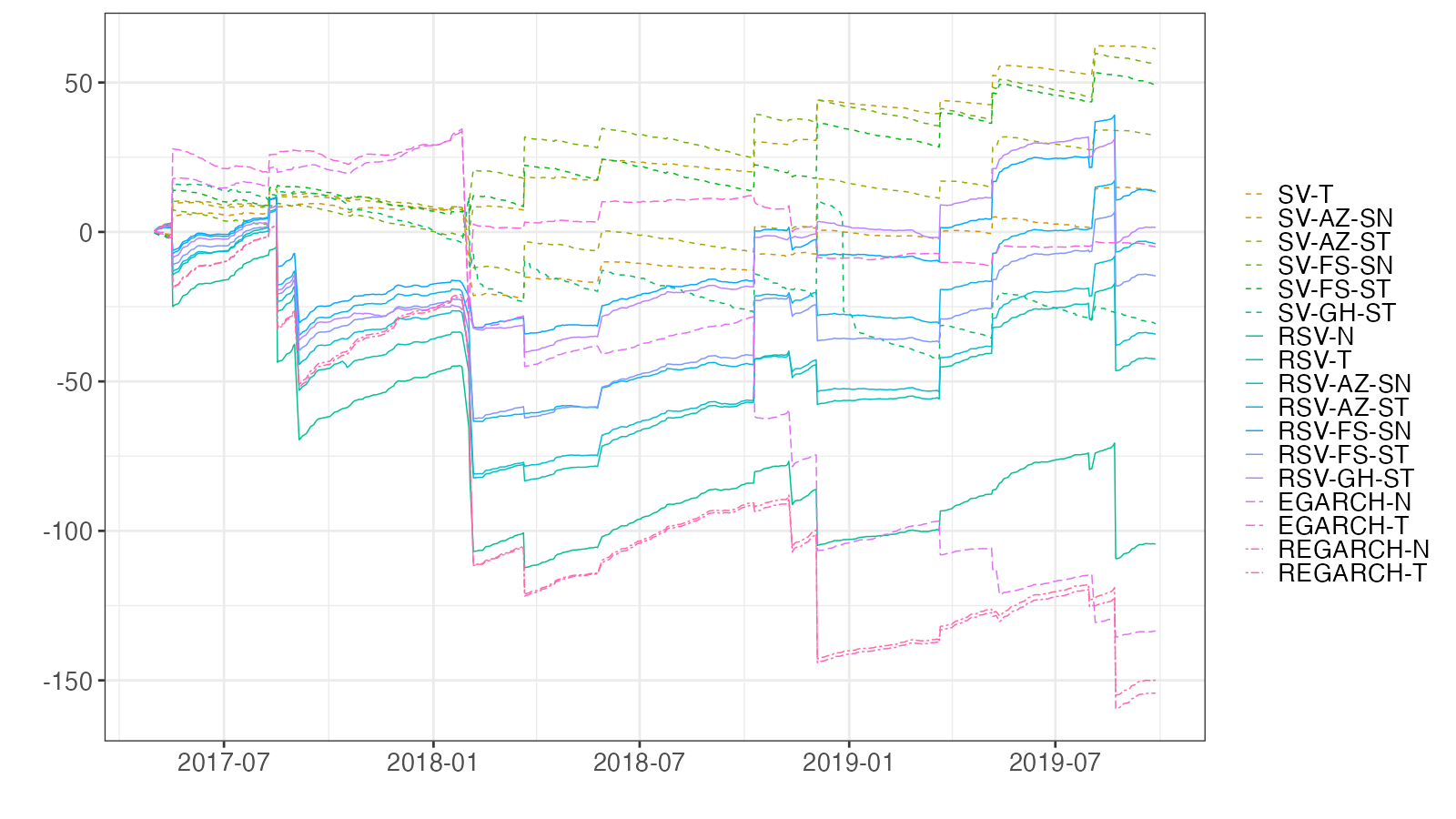
$\alpha=5\%$

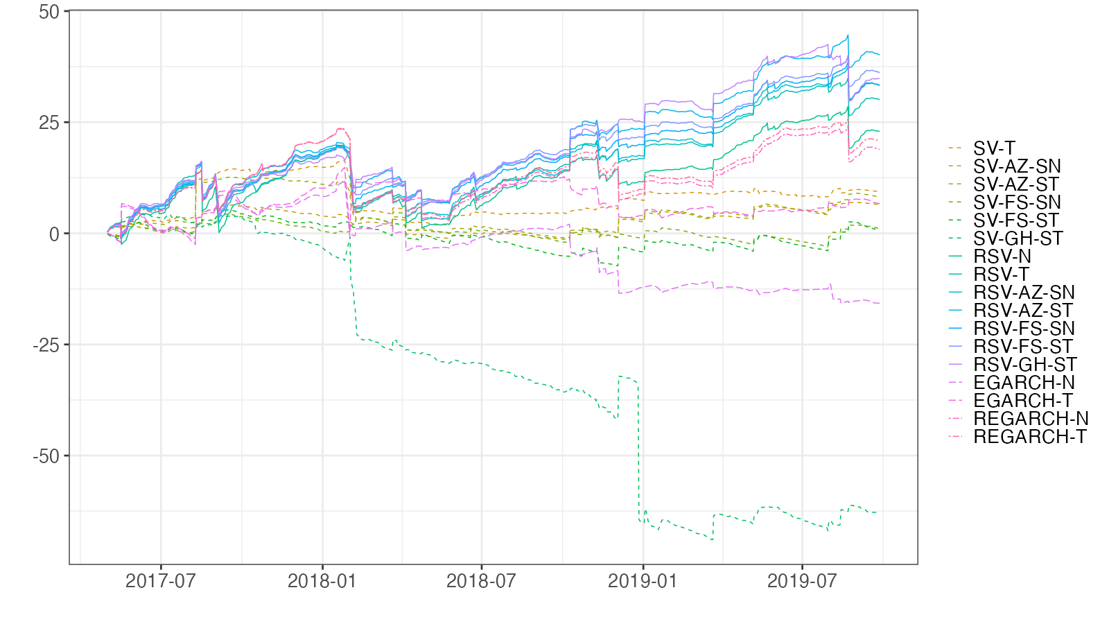
Figure 10: Cumulative loss differences (FZ0) in comparison to the SV-N model for DJIA.

The prediction results for N225 are qualitatively the same as for DJIA. Namely, they underscore the efficacy of enhancing the RSV model by integrating a skewed-heavy tail distribution into the daily return for VaR and ES forecasts. The details are provided in Appendix B.2.

4.3.3 Summary

Table 8 presents the rankings of average losses for volatility, VaR, and ES forecasts. The average ranking in the last column indicates superior performance of the RSV models compared to other models, with the RSV-FS-SN model ranking as the best. In summary, our analysis reveals that RV is a valuable predictor for volatility, VaR, and ES forecasts. Additionally, the RSV model shows greater effectiveness than the REGARCH model. Furthermore, incorporating skewed $t$-distributions into the RSV model appears to enhance forecast accuracy.

Table 8: Ranking of average losses for volatility, VaR, and ES forecasts

	DJIA					N225
	MSE	QLIKE	FZ01%	FZ05%		MSE	QLIKE	FZ01%	FZ05%		Avg
SV-N	6	13	8	16		6	11	12	14		$10.75$
SV-T	15	12	5	10		9	13	15	9		$11.00$
SV-AZ-SN	3	11	1	13		1	10	13	15		$8.38$
SV-AZ-ST	13	10	4	11		10	12	14	13		$10.88$
SV-FS-SN	14	15	2	14		14	14	11	12		$12.00$
SV-FS-ST	17	16	3	15		15	16	10	11		$12.88$
SV-GH-ST	18	14	12	18		18	15	17	18		$16.25$
RSV-N	2	2	15	7		3	3	6	4		$5.25$
RSV-T	9	7	14	6		7	6	3	2		$6.75$
RSV-AZ-SN	10	3	13	5		5	5	8	5		$6.75$
RSV-AZ-ST	12	5	9	1		8	7	2	3		$5.88$
RSV-FS-SN	1	1	6	4		2	2	7	7		$3.75$
RSV-FS-ST	5	4	11	2		4	4	4	6		$5.00$
RSV-GH-ST	8	6	7	3		11	1	1	1		$4.75$
EGARCH-N	11	17	16	17		17	17	18	17		$16.25$
EGARCH-T	16	18	10	12		16	18	16	16		$15.25$
REGARCH-N	4	8	18	9		13	9	9	10		$10.00$
REGARCH-T	7	9	17	8		12	8	5	8		$9.25$

Notes: MSE denotes Mean Squared Error for volatility forecasts; QLIKE represents Gaussian Quasi Likelihood for volatility forecasts; FZ0_1% and FZ0_5% are FZ0 loss functions for VaR and ES forecasts at $\alpha=1\%$ and $5\%$, respectively; Avg indicates the average rank across all categories.

5 Conclusion

This study has systematically analyzed the performance of various models in forecasting volatility, VaR, and ES for financial indices, specifically focusing on the DJIA and N225 indices. Our comprehensive evaluation, as presented in Table 8, demonstrates that the RSV models consistently outperform other competing models in terms of average ranking losses for volatility, VaR, and ES forecasts.

Particularly noteworthy is the superior performance of the RSV-FS-SN model, which ranks as the best among all evaluated models. This finding underscores the effectiveness of incorporating RV into forecasting models. Moreover, the comparative analysis between RSV and REGARCH models reveals that the RSV models exhibit enhanced predictive capabilities.

An important contribution of our study is the validation of the benefit of integrating skewed $t$-distributions into these forecasting models. This integration has shown a marked improvement in forecast accuracy, thereby providing a significant insight into the methodology of financial forecasting.

In conclusion, our results suggest that for accurate and reliable forecasts of volatility, VaR, and ES, the RSV models, particularly when augmented with skewed $t$-distributions, offer a robust and effective approach. These findings have important implications for risk management and financial decision-making, highlighting the critical role of model selection and the incorporation of appropriate statistical distributions in enhancing forecast precision.

Appendix

Appendix A MCMC Sampling Scheme

A.1 RSV-AZ-ST Model

The joint probability density of $(y_{t},h_{t+1})$ is given by

$$f(y_{t},h_{t+1}|z_{0t},h_{t},\bm{\theta})= \frac{1}{2\pi k(\delta)\sqrt{{(1-\rho^{2})\sigma^{2}}}}\sqrt{\frac{\mu_{\lambda}}{\lambda_{t}}}\exp\left[-\frac{1}{2}h_{t}\right]$$

$$\times\exp\left[-\frac{\mu_{\lambda}\exp(-h_{t})}{2\lambda_{t}k(\delta)^{2}(1-\rho^{2})}\left\{y_{t}-\sqrt{\frac{\lambda_{t}}{\mu_{\lambda}}}\frac{\exp(h_{t}/2)\delta[z_{0t}-c]}{\sqrt{1-c^{2}\delta^{2}}}\right.\right.$$

$$\hskip 128.0374pt-\sqrt{\frac{\lambda_{t}}{\mu_{\lambda}}}\rho\exp(h_{t}/2)k(\delta)\sigma^{-1}(h_{t+1}-\mu-\phi[h_{t}-\mu])\bigg{\}}^{2}\Bigg{]}$$

$$\times\exp\left[-\frac{1}{2\sigma^{2}}\{h_{t+1}-\mu-\phi[h_{t}-\mu]\}^{2}\right],$$

where

$$k(\delta)=\sqrt{\frac{1-\delta^{2}}{1-c^{2}\delta^{2}}}.$$

Then, the augmented joint posterior probability density is given by

$$\pi(\bm{h},\bm{\theta},\bm{z}_{0},\bm{\lambda}|\bm{x},\bm{y})\propto k(\delta)^{-T}(1-\rho^{2})^{-\frac{T-1}{2}}\sigma^{-T}(1-\phi^{2})^{\frac{1}{2}}$$

$$\times\exp\left\{-\frac{1}{2}\sum_{t=1}^{T}h_{t}-\frac{\mu_{\lambda}\exp(-h_{T})}{2\lambda_{T}k(\delta)^{2}}\left[y_{T}-\sqrt{\frac{\lambda_{T}}{\mu_{\lambda}}}\frac{\exp(h_{T}/2)\delta[z_{0T}-c]}{\sqrt{1-c^{2}\delta^{2}}}\right]^{2}\right\}$$

$$\times\exp\left[-\sum_{t=1}^{T-1}\frac{\mu_{\lambda}\exp(-h_{t})}{2\lambda_{t}k(\delta)^{2}(1-\rho^{2})}\left\{y_{t}-\sqrt{\frac{\lambda_{t}}{\mu_{\lambda}}}\frac{\exp(h_{t}/2)\delta[z_{0t}-c]}{\sqrt{1-c^{2}\delta^{2}}}\right.\right.$$

$$\hskip 145.10922pt-\sqrt{\frac{\lambda_{t}}{\mu_{\lambda}}}\rho\exp(h_{t}/2)k(\delta)\sigma^{-1}(h_{t+1}-\mu-\phi[h_{t}-\mu])\bigg{\}}^{2}\bigg{]}$$

$$\times\exp\left[-\frac{1}{2\sigma^{2}}\sum_{t=1}^{T-1}\{h_{t+1}-\mu-\phi[h_{t}-\mu]\}^{2}-\frac{(1-\phi^{2})}{2\sigma^{2}}(h_{1}-\mu)^{2}\right]$$

$$\times\exp\left\{-\frac{1}{2}\sum_{t=1}^{T}z_{0t}^{2}I(z_{0t}>0)\right\}\times\prod_{t=1}^{T}\frac{\mu_{\lambda}^{\frac{1}{2}}\left(\frac{\nu}{2}\right)^{\frac{\nu}{2}}}{\Gamma\left(\frac{\nu}{2}\right)}\lambda_{t}^{-\frac{\nu+1}{2}-1}\exp\left(-\frac{\nu}{2\lambda_{t}}\right)$$

$$\times\sigma_{u}^{-T}\times\exp\left\{-\frac{1}{2\sigma_{u}^{2}}\sum_{t=1}^{T}(x_{t}-\xi-h_{t})^{2}\right\}\times\pi(\bm{\theta}),$$

where $\pi(\bm{\theta})$ is a prior probability density function of $\bm{\theta}$.

A.1.1 Generation of $\mu$

The conditional posterior distribution of $\mu$ is normal, $\mu|\cdot\sim N(\mu_{1},\sigma_{\mu 1}^{2})$ where

$$\sigma_{\mu 1}^{-2} =\sigma_{\mu 0}^{-2}+\sigma^{-2}[1-\phi^{2}+(T-1)(1-\phi)^{2}(1-\rho^{2})^{-1}],$$

$$\mu_{1} =\sigma_{\mu 1}^{2}\left\{\sigma_{\mu 0}^{-2}\mu_{0}+\sigma^{-2}\left[(1-\phi^{2})h_{1}+\frac{1-\phi}{1-\rho^{2}}\sum_{t=1}^{T-1}\left\{h_{t+1}-\phi h_{t}\right.\right.\right.$$

$$\hskip 133.72786pt\left.\left.\left.-\sqrt{\frac{\mu_{\lambda}}{\lambda_{t}}}\frac{\rho\sigma\exp(-h_{t}/2)}{k(\delta)}\left(y_{t}-\sqrt{\frac{\lambda_{t}}{\mu_{\lambda}}}\frac{\exp(h_{t}/2)\delta[z_{0t}-c]}{\sqrt{1-c^{2}\delta^{2}}}\right)\right\}\right]\right\}.$$

A.1.2 Generation of $\phi$

The conditional posterior density of $\phi$ is

$$\pi(\phi|\cdot)\propto (1+\phi)^{a_{\phi 0}-1}(1-\phi)^{b_{\phi 0}-1}(1-\phi^{2})^{\frac{1}{2}}$$

$$\times\exp\left[-\sum_{t=1}^{T-1}\frac{\mu_{\lambda}\exp(-h_{t})}{2\lambda_{t}k(\delta)^{2}(1-\rho^{2})}\left\{y_{t}-\sqrt{\frac{\lambda_{t}}{\mu_{\lambda}}}\frac{\exp(h_{t}/2)\delta[z_{0t}-c]}{\sqrt{1-c^{2}\delta^{2}}}\right.\right.$$

$$\hskip 142.26378pt-\sqrt{\frac{\lambda_{t}}{\mu_{\lambda}}}\rho\exp(h_{t}/2)k(\delta)\sigma^{-1}(h_{t+1}-\mu-\phi[h_{t}-\mu])\bigg{\}}^{2}\Bigg{]}$$

$$\times\exp\left[-\frac{1}{2\sigma^{2}}\sum_{t=1}^{T-1}\{h_{t+1}-\mu-\phi[h_{t}-\mu]\}^{2}-\frac{(1-\phi^{2})}{2\sigma^{2}}(h_{1}-\mu)^{2}\right],$$

$$\propto g(\phi)\times\exp\left\{-\frac{1}{2\sigma_{\phi}^{2}}(\phi-\mu_{\phi})^{2}\right\},$$

where

$$g(\phi) =(1+\phi)^{a_{\phi 0}-\frac{1}{2}}(1-\phi)^{b_{\phi 0}-\frac{1}{2}},$$

$$\sigma_{\phi}^{2} =\frac{\sigma^{2}(1-\rho^{2})}{\rho^{2}(h_{1}-\mu)^{2}+\sum_{t=2}^{T-1}(h_{t}-\mu)^{2}},$$

$$\mu_{\phi} =\frac{\sigma_{\phi}^{2}}{\sigma^{2}(1-\rho^{2})}\sum_{t=1}^{T-1}\left\{h_{t+1}-\mu-\sqrt{\frac{\mu_{\lambda}}{\lambda_{t}}}\frac{\rho\sigma\exp(-h_{t}/2)}{k(\delta)}\left(y_{t}-\sqrt{\frac{\lambda_{t}}{\mu_{\lambda}}}\frac{\exp(h_{t}/2)\delta[z_{0t}-c]}{\sqrt{1-c^{2}\delta^{2}}}\right)\right\}(h_{t}-\mu).$$

Thus, we propose a candidate $\phi^{\dagger}\sim N(\mu_{\phi},\sigma_{\phi}^{2})$ and accept it with probability $\min\{1,g(\phi^{\dagger})/g(\phi)\}$.

Generation of $\sigma_{\eta}^{2}$ and $\rho$

Instead of sampling $\sigma_{\eta}^{2}$ and $\rho$ separately, we sample them jointly. Define $\vartheta=(\sigma_{\eta},\rho)^{\prime}$. Then, the conditional posterior density of $\vartheta$ is

$$\pi(\vartheta|\cdot) \propto(\sigma_{\eta}^{2})^{-\frac{n_{0}+T}{2}-1}\exp\left(-\frac{S_{0}}{2\sigma_{\eta}^{2}}\right)(1+\rho)^{a_{\rho 0}-1}(1-\rho)^{b_{\rho 0}-1}(1-\rho^{2})^{-\frac{T-1}{2}}$$

$$\quad\times\exp\left[-\sum_{t=1}^{T-1}\frac{\mu_{\lambda}\exp(-h_{t})}{2\lambda_{t}k(\delta)^{2}(1-\rho^{2})}\left\{y_{t}-\sqrt{\frac{\lambda_{t}}{\mu_{\lambda}}}\frac{\exp(h_{t}/2)\delta[z_{0t}-c]}{\sqrt{1-c^{2}\delta^{2}}}\right.\right.$$

$$\quad\hskip 145.10922pt-\sqrt{\frac{\lambda_{t}}{\mu_{\lambda}}}\rho\exp(h_{t}/2)k(\delta)\sigma_{\eta}^{-1}(h_{t+1}-\mu-\phi[h_{t}-\mu])\Bigg{\}}^{2}\Bigg{]}$$

$$\quad\times\exp\left[-\frac{1}{2\sigma_{\eta}^{2}}\sum_{t=1}^{T-1}\{h_{t+1}-\mu-\phi[h_{t}-\mu]\}^{2}-\frac{(1-\phi^{2})}{2\sigma_{\eta}^{2}}(h_{1}-\mu)^{2}\right].$$

To handle the restrictions on $\sigma_{\eta}$ and $\rho$, namely, $\sigma_{\eta}>0$ and $|\rho|<1$, we change the variables as $\omega_{1}=\log\sigma_{\eta}$ and $\omega_{2}=\log(1+\rho)-\log(1-\rho)$. Then, we can sample $\omega_{1}$ and $\omega_{2}$ without any restriction. Let $\hat{\vartheta}$ be the mode of the conditional density and $\hat{\omega}$ be the corresponding value. Then, we approximate the conditional posterior distribution by $N(\omega_{*},\sigma_{\eta*})$ where

$$\omega_{*}=\hat{\omega}+\sigma_{\eta*}\frac{\partial\log\pi(\omega|\cdot)}{\partial\omega}\Bigg{|}_{\omega=\hat{\omega}},\quad\sigma_{\eta*}^{-1}=-\frac{\partial^{2}\log\pi(\omega|\cdot)}{\partial\omega\partial\omega^{\prime}}\Bigg{|}_{\omega=\hat{\omega}}.$$

Thus, we propose a candidate $\omega^{\dagger}\sim N(\omega_{*},\sigma_{\eta*})$ and accept it with probability

$$\min\left[1,\frac{\pi(\vartheta^{\dagger}|\cdot)f_{N}(\omega|\omega_{*},\sigma_{\eta*})|J(\vartheta)|}{\pi(\vartheta|\cdot)f_{N}(\omega^{\dagger}|\omega_{*},\sigma_{\eta*})|J(\vartheta^{\dagger})|}\right],$$

where $f_{N}(\cdot|\mu,\sigma_{\eta}^{2})$ denotes the probability density of a normal distribution with mean $\mu$ and variance $\sigma_{\eta}^{2}$, and $J(\cdot)$ is the Jacobian, and $\vartheta^{\dagger}$ is the inverse transformation of $\omega^{\dagger}$.

A.1.3 Generation of $\delta$

The conditional posterior density of $\delta$ is

$$\pi(\delta|\cdot)\propto (1+\delta)^{a_{\delta 0}-1}(1-\delta)^{b_{\delta 0}-1}k(\delta)^{-T}$$

$$\times\exp\left\{-\frac{\mu_{\lambda}\exp(-h_{T})}{2\lambda_{T}k(\delta)^{2}}\left[y_{T}-\sqrt{\frac{\lambda_{T}}{\mu_{\lambda}}}\frac{\exp(h_{T}/2)\delta[z_{0T}-c]}{\sqrt{1-c^{2}\delta^{2}}}\right]^{2}\right\}$$

$$\times\exp\left[-\sum_{t=1}^{T-1}\frac{\mu_{\lambda}\exp(-h_{t})}{2\lambda_{t}k(\delta)^{2}(1-\rho^{2})}\left\{y_{t}-\sqrt{\frac{\lambda_{t}}{\mu_{\lambda}}}\frac{\exp(h_{t}/2)\delta[z_{0t}-c]}{\sqrt{1-c^{2}\delta^{2}}}\right.\right.$$

$$\hskip 145.10922pt-\sqrt{\frac{\lambda_{t}}{\mu_{\lambda}}}\rho\exp(h_{t}/2)k(\delta)\sigma^{-1}(h_{t+1}-\mu-\phi[h_{t}-\mu])\Bigg{\}}^{2}\Bigg{]}.$$

We approximate the conditional posterior distribution by $N(\hat{\delta},\sigma_{\hat{\delta}}^{2})$ where $\hat{\delta}$ is the mode of the conditional density, and $\sigma_{\hat{\delta}}^{-2}=-\frac{\partial^{2}\log\pi(\delta|\cdot)}{\partial\delta^{2}}\Big{|}_{\delta=\hat{\delta}}$. A candidate $\delta^{\dagger}\sim\mathcal{TN}_{(-1,1)}(\hat{\delta},\sigma_{\hat{\delta}}^{2})$ is proposed and accepted with probability $\min\left[1,\left\{\frac{\pi(\delta^{\dagger}|\cdot)f_{N}(\delta|\hat{\delta},\sigma_{\hat{\delta}}^{2})}{\pi(\delta|\cdot)f_{N}(\delta^{\dagger}|\hat{\delta},\sigma_{\hat{\delta}}^{2})}\right\}\right]$, where $\mathcal{TN}_{(a,b)}(\mu,\sigma^{2})$ denotes a normal distribution $N(\mu,\sigma^{2})$ truncated over $(a,b)$, and $f_{N}(\cdot|\mu,\sigma^{2})$ denotes the probability density of a normal distribution with mean $\mu$ and variance $\sigma^{2}$.

A.1.4 Generation of $\xi$

The conditional posterior distribution of $\xi$ is normal, $N(\mu_{\xi},\sigma_{\xi}^{2})$, where

$$\sigma_{\xi}^{-2} =\sigma_{\xi 0}^{-2}+T\sigma_{u}^{-2},$$

$$\mu_{\xi} =\sigma_{\xi}^{2}\left\{\sigma_{\xi 0}^{-2}\mu_{\xi 0}+\sigma_{u}^{-2}\sum_{t=1}^{T}(x_{t}-h_{t})\right\}.$$

A.1.5 Generation of $\sigma_{u}^{2}$

The conditional posterior distribution of $\sigma_{u}^{2}$ is $\mathcal{IG}(n_{u1}/2,S_{u1}/2)$ where

$$n_{u1} =n_{u0}+T,$$

$$S_{u1} =S_{u0}+\sum_{t=1}^{T}(x_{t}-\xi-h_{t})^{2}.$$

A.1.6 Generation of $\nu$

The conditional probability density function of $\nu$ is

$$\pi(\nu|\cdot)\propto \exp\left\{\frac{T}{2}\log\mu_{\lambda}+\frac{\nu T}{2}\log\left(\frac{\nu}{2}\right)-T\log\Gamma\left(\frac{\nu}{2}\right)-\frac{\nu}{2}\sum_{t=1}^{T}(\lambda_{t}^{-1}+\log\lambda_{t})+(n_{\nu 0}-1)\log\nu-S_{\nu 0}\nu\right\}$$

$$\times\exp\left[-\sum_{t=1}^{T-1}\frac{\mu_{\lambda}\exp(-h_{t})}{2\lambda_{t}k(\delta)^{2}(1-\rho^{2})}\left\{y_{t}-\sqrt{\frac{\lambda_{t}}{\mu_{\lambda}}}\frac{\exp(h_{t}/2)\delta[z_{0t}-c]}{\sqrt{1-c^{2}\delta^{2}}}\right.\right.$$

$$\hskip 145.10922pt-\sqrt{\frac{\lambda_{t}}{\mu_{\lambda}}}\rho\exp(h_{t}/2)k(\delta)\sigma^{-1}(h_{t+1}-\mu-\phi[h_{t}-\mu])\Bigg{\}}^{2}\Bigg{]}$$

$$\times\exp\left[-\frac{\mu_{\lambda}\exp(-h_{T})}{2\lambda_{T}k(\delta)^{2}}\left\{y_{T}-\sqrt{\frac{\lambda_{T}}{\mu_{\lambda}}}\frac{\exp(h_{T}/2)\delta[z_{0T}-c]}{\sqrt{1-c^{2}\delta^{2}}}\right\}^{2}\right].$$

We approximate the conditional density by a normal density around the mode and conduct a Metropolis-Hastings (MH) algorithm as in the generation of $\delta$.

A.1.7 Generation of $\bm{z}_{0}$

The conditional posterior distribution of $z_{0t}$ is $\mathcal{TN}_{(0,\infty)}(\mu_{zt},\sigma_{zt}^{2})$ where

$$\sigma_{zt}^{-2} =\begin{cases}1+\frac{\delta^{2}}{(1-\delta^{2})(1-\rho^{2})},&t=1,\ldots,T-1,\\ \frac{1}{1-\delta^{2}},&t=T,\end{cases}$$

$$\mu_{zt} =\begin{cases}\sigma_{zt}^{2}\sqrt{\frac{\mu_{\lambda}}{\lambda_{t}}}\frac{\exp(-h_{t}/2)\delta}{k(\delta)^{2}(1-\rho^{2})\sqrt{1-c^{2}\delta^{2}}}\left[y_{t}+\sqrt{\frac{\lambda_{t}}{\mu_{\lambda}}}\frac{\exp(h_{t}/2)c\delta}{\sqrt{1-c^{2}\delta^{2}}}\right.\\ \hskip 133.72786pt-\sqrt{\frac{\lambda_{t}}{\mu_{\lambda}}}\rho\exp(h_{t}/2)k(\delta)\sigma^{-1}(h_{t+1}-\mu-\phi[h_{t}-\mu]),&t=1,\ldots,T-1,\\ \sigma_{zT}^{2}\sqrt{\frac{\mu_{\lambda}}{\lambda_{T}}}\frac{\exp(-h_{T}/2)\delta}{k(\delta)^{2}\sqrt{1-c^{2}\delta^{2}}}\left[y_{T}+\sqrt{\frac{\lambda_{T}}{\mu_{\lambda}}}\frac{\exp(h_{T}/2)c\delta}{\sqrt{1-c^{2}\delta^{2}}}\right],&t=T.\end{cases}$$

A.1.8 Generation of $\bm{h}$

First, we rewrite the RSV-AZ-ST model (12), (13), (14), and (30) as

$$x_{t} =\mu_{x}+\alpha_{t}+u_{t},\quad t=1,\ldots,n,$$ (69)

$$y_{t} =(\delta\bar{z}_{0t}+\sqrt{1-\delta^{2}}z_{t})\sqrt{\lambda_{t}}\exp(\alpha_{t}/2)\gamma,\quad t=1,\ldots,n,$$ (70)

$$\alpha_{t+1} =\phi\alpha_{t}+\eta_{t},\quad t=0,\ldots,n-1,$$ (71)

where

$$\mu_{x}=\xi+\mu,\quad\alpha_{t} =h_{t}-\mu,\quad\bar{z}_{0t}=z_{0t}-c,\quad\gamma=\frac{\exp(\mu/2)}{\sqrt{(1-c^{2}\delta^{2})\mu_{\lambda}}}.$$ (72)

The log-likelihood of $(y_{t},x_{t})$ given $\alpha_{t}$, $\alpha_{t+1}$, and other parameters excluding the constant term is

$$l_{t} =-\frac{\alpha_{t}}{2}-\frac{(y_{t}-\mu_{t})^{2}}{2\sigma_{t}^{2}}-\frac{(x_{t}-\mu_{x}-\alpha_{t})^{2}}{2\sigma_{u}^{2}},$$ (73)

where

$$\mu_{t} =\begin{cases}\left[\delta\bar{z}_{0t}+\sqrt{1-\delta^{2}}\dfrac{\rho}{\sigma_{\eta}}(\alpha_{t+1}-\phi\alpha_{t})\right]\sqrt{\lambda_{t}}\exp(\alpha_{t}/2)\gamma,&t=1,\ldots,n-1,\\[5.0pt] \delta\bar{z}_{0t}\sqrt{\lambda_{t}}\exp(\alpha_{t}/2)\gamma,&t=n,\end{cases}$$ (74)

$$\sigma_{t}^{2} =\begin{cases}(1-\rho^{2})(1-\delta^{2})\lambda_{t}\exp(\alpha_{t})\gamma^{2},&t=1,\ldots,n-1,\\[5.0pt] (1-\delta^{2})\lambda_{t}\exp(\alpha_{t})\gamma^{2},&t=n.\end{cases}$$ (75)

Using this log-likelihood, we can efficiently sample the latent variable $(\alpha_{1},\ldots,\alpha_{n})$ via the multi-move sampler based on Omori et al. (2007), Omori and Watanabe (2008, 2015). For further details, see Takahashi et al. (2016, 2023).

A.1.9 Generation of $\bm{\lambda}$

The conditional probability density function of $\lambda_{t}$ is

$$\pi(\lambda_{t}|\cdot)\propto \lambda_{t}^{-(\frac{\nu+1}{2}+1)}\exp\left[-\frac{\nu}{2\lambda_{t}}-\frac{\mu_{\lambda}\exp(-h_{t})}{2\lambda_{t}k(\delta)^{2}(1-\rho^{2})}\left\{y_{t}-\sqrt{\frac{\lambda_{t}}{\mu_{\lambda}}}\frac{\exp(h_{t}/2)\delta[z_{0t}-c]}{\sqrt{1-c^{2}\delta^{2}}}\right.\right.$$

$$\hskip 145.10922pt-\sqrt{\frac{\lambda_{t}}{\mu_{\lambda}}}\rho\exp(h_{t}/2)k(\delta)\sigma^{-1}(h_{t+1}-\mu-\phi[h_{t}-\mu])I(t<T)\bigg{\}}^{2}\bigg{]}$$

$$\propto \lambda_{t}^{-(\frac{a}{2}+1)}\exp\left(-\frac{b_{t}}{2\lambda_{t}}\right)\times g(\lambda_{t})$$

where

$$a =\nu+1,$$

$$b_{t} =\begin{cases}\nu+\frac{\mu_{\lambda}\exp(-h_{t})y_{t}^{2}}{k(\delta)^{2}(1-\rho^{2})},&t=1,\ldots,n-1,\\ \nu+\frac{\mu_{\lambda}\exp(-h_{t})y_{t}^{2}}{k(\delta)^{2}},&t=n,\end{cases}$$

$$g(\lambda_{t}) =\begin{cases}\exp\left[\sqrt{\frac{\mu_{\lambda}}{\lambda_{t}}}\frac{\exp(-h_{t}/2)y_{t}}{k(\delta)^{2}(1-\rho^{2})}\left\{\frac{\delta[z_{0t}-c]}{\sqrt{1-c^{2}\delta^{2}}}+\rho k(\delta)\sigma^{-1}(h_{t+1}-\mu-\phi[h_{t}-\mu])\right\}\right],&t=1,\ldots,n-1,\\ \exp\left[\sqrt{\frac{\mu_{\lambda}}{\lambda_{t}}}\frac{\exp(-h_{t}/2)y_{t}}{k(\delta)^{2}}\frac{\delta[z_{0t}-c]}{\sqrt{1-c^{2}\delta^{2}}}\right\},&t=n,\end{cases}$$

We propose a candidate from the inverse Gamma distribution, $\lambda_{t}^{\dagger}\sim\mathcal{IG}(a/2,b_{t}/2)$, and accept it with probability $\min\{1,g(\lambda_{t}^{\dagger})/g(\lambda_{t})\}$.

A.2 RSV-FS-ST Model

The joint probability density of $(y_{t},h_{t+1})$ is given by

$$f(y_{t},h_{t+1}|\bm{\theta},\lambda_{t})= q_{T}\left(y_{t}\exp(-h_{t}/2)|\gamma,\nu\right)\exp\left(-\frac{1}{2}h_{t}\right)$$

$$\times\frac{1}{\sqrt{2\pi(1-\rho^{2})\sigma^{2}}}\exp\left[-\frac{1}{2(1-\rho^{2})\sigma^{2}}\left\{h_{t+1}-\mu-\phi[h_{t}-\mu]-\rho\sigma\exp(-h_{t}/2)y_{t}\right\}^{2}\right],$$

where $q_{T}$ is defined in (46). Then, the joint posterior probability density is given by

$$\pi(\bm{h},\bm{\theta}|\bm{x},\bm{y})\propto (1-\rho^{2})^{-\frac{T-1}{2}}\sigma^{-T}(1-\phi^{2})^{-\frac{1}{2}}\times\prod_{t=1}^{T}q_{T}\left(y_{t}\exp(-h_{t}/2)|\gamma,\nu\right)\times\exp\left(-\frac{1}{2}\sum_{t=1}^{T}h_{t}\right)$$

$$\times\exp\left[-\frac{1}{2(1-\rho^{2})\sigma^{2}}\sum_{t=1}^{T-1}\left\{h_{t+1}-\mu-\phi[h_{t}-\mu]-\rho\sigma\exp(-h_{t}/2)y_{t}\right\}^{2}\right]$$

$$\times\exp\left[-\frac{(1-\phi^{2})}{2\sigma^{2}}(h_{1}-\mu)^{2}\right]\times\sigma_{u}^{-T}\times\exp\left\{-\frac{1}{2\sigma_{u}^{2}}\sum_{t=1}^{T}(x_{t}-\xi-h_{t})^{2}\right\}\times\pi(\bm{\theta}).$$

A.2.1 Generation of $\mu$

The conditional posterior distribution of $\mu$ is normal, $\mu|\cdot\sim N(\mu_{1},\sigma_{\mu 1}^{2})$ where

$$\sigma_{\mu 1}^{-2} =\sigma_{\mu 0}^{-2}+\sigma^{-2}\left[1-\phi^{2}+(T-1)(1-\phi)^{2}(1-\rho^{2})^{-1}\right],$$

$$\mu_{1} =\sigma_{\mu 1}^{2}\left[\sigma_{\mu 0}^{-2}\mu_{0}+\sigma^{-2}\left\{(1-\phi^{2})h_{1}+\frac{1-\phi}{1-\rho^{2}}\sum_{t=1}^{T-1}\left(h_{t+1}-\phi h_{t}-\rho\sigma\exp(-h_{t}/2)y_{t}\right)\right\}\right].$$

A.2.2 Generation of $\phi$

The conditional posterior density of $\phi$ is

$$\pi(\phi|\cdot)\propto (1-\phi)^{a_{\phi 0}-1}(1+\phi)^{b_{\phi 0}-1}(1-\phi^{2})^{\frac{1}{2}}$$

$$\times\exp\left[-\frac{1}{2(1-\rho^{2})\sigma^{2}}\sum_{t=1}^{T-1}\left\{h_{t+1}-\mu-\phi(h_{t}-\mu)-\rho\sigma\exp(-h_{t}/2)y_{t}\right\}^{2}\right]$$

$$\times\exp\left[-\frac{(1-\phi^{2})}{2\sigma^{2}}(h_{1}-\mu)^{2}\right]$$

$$\propto k(\phi)\times\exp\left\{-\frac{1}{2\sigma_{\phi}^{2}}(\phi-\mu_{\phi})^{2}\right\},$$

where

$$k(\phi) =(1-\phi)^{a_{\phi 0}-\frac{1}{2}}(1+\phi)^{b_{\phi 0}-\frac{1}{2}},$$

$$\sigma_{\phi}^{2} =\frac{\sigma^{2}(1-\rho^{2})}{\rho^{2}(h_{1}-\mu)^{2}+\sum_{t=2}^{T-1}(h_{t}-\mu)^{2}},$$

$$\mu_{\phi} =\frac{\sigma_{\phi}^{2}}{\sigma^{2}(1-\rho^{2})}\sum_{t=1}^{T-1}\left\{h_{t+1}-\mu-\rho\sigma\exp(-h_{t}/2)y_{t}\right\}(h_{t}-\mu).$$

Thus, we apply the MH algorithm. We propose a candidate $\phi^{\dagger}\sim N(\mu_{\phi},\sigma_{\phi}^{2})$ and accept it with probability $\min\{1,k(\phi^{\dagger})/k(\phi)\}$.

A.2.3 Generation of $\rho$

The conditional posterior density of $\rho$ is

$$\pi(\rho|\cdot)\propto (1+\rho)^{a_{\rho 0}-1}(1-\rho)^{b_{\rho 0}-1}(1-\rho^{2})^{-\frac{T-1}{2}}$$

$$\times\exp\left[-\frac{1}{2(1-\rho^{2})\sigma^{2}}\sum_{t=1}^{T-1}\left\{h_{t+1}-\mu-\phi(h_{t}-\mu)-\rho\sigma\exp(-h_{t}/2)y_{t}\right\}^{2}\right].$$

We approximate the conditional posterior distribution by $N(\hat{\rho},\sigma_{\hat{\rho}}^{2})$ where $\hat{\rho}$ is the mode of the conditional density and $\sigma_{\hat{\rho}}^{-2}=-\frac{\partial^{2}\log\pi(\rho|\cdot)}{\partial\rho^{2}}\big{|}_{\rho=\hat{\rho}}$. Propose a candidate $\rho^{\dagger}\sim\mathcal{TN}_{(-1,1)}(\hat{\rho},\sigma_{\hat{\rho}}^{2})$ and accept it with probability $\min\left[1,\frac{\pi(\rho^{\dagger}|\cdot)f_{N}(\rho|\hat{\rho},\sigma_{\hat{\rho}}^{2})}{\pi(\rho|\cdot)f_{N}(\rho^{\dagger}|\hat{\rho},\sigma_{\hat{\rho}}^{2})}\right]$.

A.2.4 Generation of $\sigma^{2}$

The conditional posterior density of $\sigma^{2}$ is

$$\pi(\sigma^{2}|\cdot)\propto (\sigma^{2})^{-\frac{n_{0}+T}{2}-1}\exp\left(-\frac{S_{0}}{2\sigma^{2}}\right)\times\exp\left[-\frac{(1-\phi^{2})}{2\sigma^{2}}(h_{1}-\mu)^{2}\right]$$

$$\times\exp\left[-\frac{1}{2(1-\rho^{2})\sigma^{2}}\sum_{t=1}^{T-1}\left\{h_{t+1}-\mu-\phi(h_{t}-\mu)-\rho\sigma\exp(-h_{t}/2)y_{t}\right\}^{2}\right]$$

$$\propto k(\sigma^{2})\times(\sigma^{2})^{-\frac{n_{1}}{2}-1}\exp\left(-\frac{S_{1}}{2\sigma^{2}}\right),$$

where

$$n_{1} =n_{0}+T,$$

$$S_{1} =S_{0}+(1-\phi^{2})(h_{1}-\mu)^{2}+\frac{1}{1-\rho^{2}}\sum_{t=1}^{T-1}\{h_{t+1}-\mu-\phi(h_{t}-\mu)\}^{2},$$

$$k(\sigma^{2}) =\exp\left[\sigma^{-1}\sum_{t=1}^{T-1}\frac{\rho y_{t}\exp(-h_{t}/2)}{1-\rho^{2}}\left\{h_{t+1}-\mu-\phi(h_{t}-\mu)\right\}\right].$$

Thus, we propose a candidate $\sigma^{2\dagger}\sim\mathcal{IG}(n_{1}/2,S_{1}/2)$ and accept it with probability $\min\{1,k(\sigma^{2\dagger})/k(\sigma^{2})\}$.

A.2.5 Generation of $\xi$

The conditional posterior distribution of $\xi$ is normal, $N(\mu_{\xi},\sigma_{\xi}^{2})$, where

$$\sigma_{\xi}^{-2} =\sigma_{\xi 0}^{-2}+T\sigma_{u}^{-2},$$

$$\mu_{\xi} =\sigma_{\xi}^{2}\left[\sigma_{\xi 0}^{-2}\mu_{\xi 0}+\sigma_{u}^{-2}\sum_{t=1}^{T}(x_{t}-h_{t})\right].$$

A.2.6 Generation of $\sigma_{u}^{2}$

The conditional posterior distribution of $\sigma_{u}^{2}$ is $\mathcal{IG}(n_{u1}/2,S_{u1}/2)$ where

$$n_{u1} =n_{u0}+T,$$

$$S_{u1} =S_{u0}+\sum_{t=1}^{T}(x_{t}-\xi-h_{t})^{2}.$$

A.2.7 Generation of $\gamma$

The conditional posterior density of $\gamma$ is

$$\pi(\gamma|\cdot)\propto \exp\left\{(n_{\gamma 0}-1)\log\gamma-S_{\gamma 0}\gamma+\sum_{t=1}^{T}\log q_{T}\left(y_{t}\exp(-h_{t}/2)|\gamma,\nu\right)\right\}.$$

We consider a transformation $\tilde{\gamma}=\log\gamma$, and conduct a random walk MH algorithm for $\tilde{\gamma}$ (so that we add a Jacobian term $\tilde{\gamma}$ to the log conditional posterior density).

A.2.8 Generation of $\nu$

The conditional probability density function of $\nu$ is

$$\pi(\nu|\cdot)\propto\exp\left\{(n_{\nu 0}-1)\log\nu-S_{\nu 0}\nu+\sum_{t=1}^{T}\log q_{T}\left(y_{t}\exp(-h_{t}/2)|\gamma,\nu\right)\right\}.$$

We consider a transformation $\tilde{\nu}=\log(\nu-2)$, and conduct a random walk MH algorithm for $\tilde{\nu}$ (so that we add a Jacobian term $\tilde{\nu}$ to the log conditional posterior density).

A.2.9 Generation of $\bm{h}$

First we define

$$g(h_{t}|\gamma,\nu) =-\frac{\nu+1}{2}\log\left[1+\frac{\left(\sigma_{*}y_{t}\exp(-h_{t}/2)+\mu_{*}\right)^{2}}{\nu}\left\{\gamma^{-2}I\left(y_{t}\exp(-h_{t}/2)\geq-\frac{\mu_{*}}{\sigma_{*}}\right)\right.\right.$$

$$\hskip 170.71652pt\left.\left.+\gamma^{2}I\left(y_{t}\exp(-h_{t}/2)<-\frac{\mu_{*}}{\sigma_{*}}\right)\right\}\right].$$

(1) For $t=1$, the conditional posterior density of $h_{1}$ is

$$\pi(h_{1}|\cdot) \propto\exp\left[g(h_{1}|\gamma,\nu)-\frac{1}{2(1-\rho^{2})\sigma^{2}}\left\{h_{2}-\mu-\phi(h_{1}-\mu)-\rho\sigma\exp(-h_{1}/2)y_{1}\right\}^{2}\right]$$

$$\times\exp\left[-\frac{1}{2}h_{1}-\frac{(1-\phi^{2})}{2\sigma^{2}}(h_{1}-\mu)^{2}-\frac{1}{2\sigma_{u}^{2}}(x_{1}-\xi-h_{1})^{2}\right].$$

Define

$$\sigma_{h1}^{-2} =\sigma^{-2}\left\{1-\phi^{2}+\frac{\phi^{2}}{1-\rho^{2}}\right\}+\sigma_{u}^{-2},$$

$$\mu_{h1} =\sigma_{h1}^{2}\left[-\frac{1}{2}+\frac{\phi\{h_{2}-(1-\phi)\mu\}}{\sigma^{2}(1-\rho^{2})}+\frac{(1-\phi^{2})\mu}{\sigma^{2}}+\frac{x_{1}-\xi}{\sigma_{u}^{2}}\right],$$

$$k(h_{1}) =\exp\left[g(h_{1}|\gamma,\nu)+\frac{\rho y_{1}\exp(-h_{1}/2)}{(1-\rho^{2})\sigma}\left\{h_{2}-\mu-\phi(h_{1}-\mu)\right\}-\frac{\rho^{2}y_{1}^{2}\exp(-h_{1})}{2(1-\rho^{2})}\right].$$

Thus we propose a candidate $h_{1}^{\dagger}\sim N(\mu_{h1},\sigma_{h1}^{2})$ and accept it with probability $\min\{1,k(h_{1}^{\dagger})/k(h_{1})\}$.

(2) For $t=2,\ldots,T-1$, the conditional posterior density of $h_{t}$ is

$$\pi(h_{t}|\cdot) \propto\exp\left[g(h_{t}|\gamma,\nu)-\frac{1}{2(1-\rho^{2})\sigma^{2}}\left\{h_{t+1}-\mu-\phi(h_{t}-\mu)-\rho\sigma\exp(-h_{t}/2)y_{t}\right\}^{2}\right]$$

$$\times\exp\left[-\frac{1}{2(1-\rho^{2})\sigma^{2}}\left\{h_{t}-\mu-\phi(h_{t-1}-\mu)-\rho\sigma\exp(-h_{t-1}/2)y_{t-1}\right\}^{2}\right]$$

$$\times\exp\left[-\frac{1}{2}h_{t}-\frac{1}{2\sigma_{u}^{2}}(x_{t}-\xi-h_{t})^{2}\right].$$

Define

$$\sigma_{ht}^{-2} =\sigma^{-2}\left(\frac{1+\phi^{2}}{1-\rho^{2}}\right)+\sigma_{u}^{-2},$$

$$\mu_{ht} =\sigma_{ht}^{2}\left[-\frac{1}{2}+\frac{\phi\{h_{t+1}-(1-\phi)\mu\}}{\sigma^{2}(1-\rho^{2})}+\frac{\{(1-\phi)\mu+\phi h_{t-1}\}}{\sigma^{2}(1-\rho^{2})}+\frac{\rho y_{t-1}\exp(-h_{t-1}/2)}{(1-\rho^{2})\sigma}+\frac{x_{t}-\xi}{\sigma_{u}^{2}}\right],$$

$$k(h_{t}) =\exp\left[g(h_{t}|\gamma,\nu)-\frac{\rho^{2}y_{t}^{2}\exp(-h_{t})}{2(1-\rho^{2})}+\frac{\rho y_{t}\exp(-h_{t}/2)}{(1-\rho^{2})\sigma}\left\{h_{t+1}-\mu-\phi(h_{t}-\mu)\right\}\right].$$

Thus we propose a candidate $h_{t}^{\dagger}\sim N(\mu_{ht},\sigma_{ht}^{2})$ and accept it with probability $\min\{1,k(h_{t}^{\dagger})/g(h_{t})\}$.

(3) For $t=T$, the conditional posterior density of $h_{T}$ is

$$\pi(h_{T}|\cdot) \propto\exp\left[g(h_{T}|\gamma,\nu)-\frac{1}{2(1-\rho^{2})\sigma^{2}}\left\{h_{T}-\mu-\phi(h_{T-1}-\mu)-\rho\sigma\exp(-h_{T-1}/2)y_{T-1}\right\}^{2}\right]$$

$$\times\exp\left[-\frac{1}{2}h_{T}-\frac{1}{2\sigma_{u}^{2}}(x_{T}-\xi-h_{T})^{2}\right].$$

Define

$$\sigma_{hT}^{-2} =\sigma^{-2}(1-\rho^{2})^{-1}+\sigma_{u}^{-2},$$

$$\mu_{hT} =\sigma_{hT}^{2}\left[-\frac{1}{2}+\frac{(1-\phi)\mu+\phi h_{T-1}}{\sigma^{2}(1-\rho^{2})}+\frac{\rho y_{T-1}\exp(-h_{T-1}/2)}{(1-\rho^{2})\sigma}+\frac{x_{T}-\xi}{\sigma_{u}^{2}}\right],$$

$$k(h_{T}) =\exp\left\{g(h_{T}|\gamma,\nu)\right\}.$$

Thus we propose a candidate $h_{T}^{\dagger}\sim N(\mu_{hT},\sigma_{hT}^{2})$ and accept it with probability $\min\{1,k(h_{T}^{\dagger})/k(h_{T})\}$.

Appendix B Prediction Results for Nikkei 225 Index

B.1 Volatility Forecasts

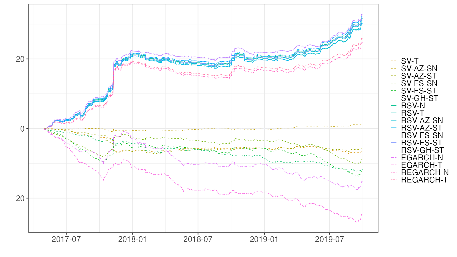
Figure 11: Cumulative loss differences (QLIKE) in comparison to the SV-N model for N225.

Tables 9 and 10 present the volatility forecasts for N225. While the SV-AZ-SN model boasts the lowest MSE, the RSV-GH-ST model exhibits the lowest QLIKE. Notably, the MSE for the SV-GH-ST model is significantly elevated compared to other models, indicating an over-prediction of volatility towards the end of 2018. Both RSV and REGARCH models outperform the SV and EGARCH models, emphasizing that the incorporation of RV refines volatility forecasts. These results mirror those obtained for DJIA. Furthermore, notable disparities emerge among models within the same category but with distinct return distributions. For instance, the RSV-FS-SN model surpasses the RSV-T, AZ-SN, and AZ-ST models in terms of performance, whereas the REGARCH-T model stands out against the REGARCH-N model. Such distinctions are visualized in Fig. 11.

Table 9: Average losses of volatility forecasts for N225

	MSE	$p_{MCS}$	QLIKE	$p_{MCS}$
SV-N	$0.4983$	$1.00^{**}$	$0.1970$	$0.00^{\hskip 5.60002pt}$
SV-T	$0.5026$	$1.00^{**}$	$0.2079$	$0.00^{\hskip 5.60002pt}$
SV-AZ-SN	$0.4844$	$1.00^{**}$	$0.1951$	$0.00^{\hskip 5.60002pt}$
SV-AZ-ST	$0.5057$	$1.00^{**}$	$0.2065$	$0.00^{\hskip 5.60002pt}$
SV-FS-SN	$0.5402$	$0.88^{**}$	$0.2119$	$0.00^{\hskip 5.60002pt}$
SV-FS-ST	$0.5428$	$0.75^{**}$	$0.2175$	$0.00^{\hskip 5.60002pt}$
SV-GH-ST	$0.6408$	$0.58^{**}$	$0.2169$	$0.00^{\hskip 5.60002pt}$
RSV-N	$0.4962$	$1.00^{**}$	$0.1434$	$0.20^{*\hskip 2.79996pt}$
RSV-T	$0.5011$	$1.00^{**}$	$0.1456$	$0.00^{\hskip 5.60002pt}$
RSV-AZ-SN	$0.4968$	$1.00^{**}$	$0.1442$	$0.00^{\hskip 5.60002pt}$
RSV-AZ-ST	$0.5017$	$1.00^{**}$	$0.1459$	$0.00^{\hskip 5.60002pt}$
RSV-FS-SN	$0.4932$	$1.00^{**}$	$0.1422$	$1.00^{**}$
RSV-FS-ST	$0.4964$	$1.00^{**}$	$0.1436$	$0.11^{*\hskip 2.79996pt}$
RSV-GH-ST	$0.5134$	$1.00^{**}$	$0.1416$	$1.00^{**}$
EGARCH-N	$0.5715$	$0.12^{*\hskip 2.79996pt}$	$0.2228$	$0.00^{\hskip 5.60002pt}$
EGARCH-T	$0.5690$	$0.00^{\hskip 5.60002pt}$	$0.2386$	$0.00^{\hskip 5.60002pt}$
REGARCH-N	$0.5236$	$1.00^{**}$	$0.1551$	$0.00^{\hskip 5.60002pt}$
REGARCH-T	$0.5205$	$1.00^{**}$	$0.1532$	$0.00^{\hskip 5.60002pt}$
Note: Refer to Table 3 for additional details.

Table 10: Summary of GW tests on QLIKE of volatility forecasts for N225

	SV-N	T	AZ-SN	AZ-ST	FS-SN	FS-ST	GH-ST	RSV-N	T	AZ-SN	AZ-ST	FS-SN	FS-ST	GH-ST	EG-N	T	REG-N	T
SV-N		$\hskip 3.49998pt18^{**}$	$\hskip 3.49998pt99^{\hskip 2.8pt}$	$\hskip 3.49998pt15^{**}$	$\hskip 3.49998pt11^{**}$	$\hskip 3.49998pt\hskip 1.99997pt8^{**}$	$\hskip 3.49998pt\hskip 1.99997pt0^{**}$	$\hskip 3.49998pt96^{**}$	$\hskip 3.49998pt96^{**}$	$\hskip 3.49998pt96^{**}$	$\hskip 3.49998pt96^{**}$	$\hskip 3.49998pt96^{**}$	$\hskip 3.49998pt96^{**}$	$\hskip 3.49998pt97^{**}$	$\hskip 3.49998pt11^{\hskip 2.8pt}$	$\hskip 3.49998pt\hskip 1.99997pt8^{**}$	$\hskip 3.49998pt96^{**}$	$\hskip 3.49998pt96^{**}$
SV-T	$\hskip 3.49998pt1.8^{\hskip 2.8pt}$		$\hskip 3.49998pt88^{*\hskip 1.39998pt}$	$\hskip 3.49998pt93^{*\hskip 1.39998pt}$	$\hskip 3.49998pt19^{\hskip 2.8pt}$	$\hskip 3.49998pt14^{\hskip 2.8pt}$	$\hskip 3.49998pt16^{\hskip 2.8pt}$	$\hskip 3.49998pt95^{**}$	$\hskip 3.49998pt95^{**}$	$\hskip 3.49998pt95^{**}$	$\hskip 3.49998pt95^{**}$	$\hskip 3.49998pt95^{**}$	$\hskip 3.49998pt95^{**}$	$\hskip 3.49998pt96^{**}$	$\hskip 3.49998pt19^{\hskip 2.8pt}$	$\hskip 3.49998pt11^{*\hskip 1.39998pt}$	$\hskip 3.49998pt94^{**}$	$\hskip 3.49998pt95^{**}$
SV-AZ-SN	$-1.0^{\hskip 2.8pt}$	$-2.0^{*\hskip 1.39998pt}$		$\hskip 3.49998pt\hskip 1.99997pt5^{*\hskip 1.39998pt}$	$\hskip 3.49998pt15^{*\hskip 1.39998pt}$	$\hskip 3.49998pt12^{**}$	$\hskip 3.49998pt\hskip 1.99997pt0^{**}$	$\hskip 3.49998pt94^{**}$	$\hskip 3.49998pt94^{**}$	$\hskip 3.49998pt94^{**}$	$\hskip 3.49998pt94^{**}$	$\hskip 3.49998pt94^{**}$	$\hskip 3.49998pt94^{**}$	$\hskip 3.49998pt95^{**}$	$\hskip 3.49998pt12^{*\hskip 1.39998pt}$	$\hskip 3.49998pt\hskip 1.99997pt9^{**}$	$\hskip 3.49998pt92^{**}$	$\hskip 3.49998pt92^{**}$
SV-AZ-ST	$\hskip 3.49998pt1.7^{\hskip 2.8pt}$	$-0.5^{\hskip 2.8pt}$	$\hskip 3.49998pt2.1^{*\hskip 1.39998pt}$		$\hskip 3.49998pt17^{\hskip 2.8pt}$	$\hskip 3.49998pt14^{\hskip 2.8pt}$	$\hskip 3.49998pt\hskip 1.99997pt1^{**}$	$\hskip 3.49998pt95^{**}$	$\hskip 3.49998pt95^{**}$	$\hskip 3.49998pt95^{**}$	$\hskip 3.49998pt95^{**}$	$\hskip 3.49998pt95^{**}$	$\hskip 3.49998pt95^{**}$	$\hskip 3.49998pt96^{**}$	$\hskip 3.49998pt17^{\hskip 2.8pt}$	$\hskip 3.49998pt12^{**}$	$\hskip 3.49998pt94^{**}$	$\hskip 3.49998pt94^{**}$
SV-FS-SN	$\hskip 3.49998pt1.7^{\hskip 2.8pt}$	$\hskip 3.49998pt0.3^{\hskip 2.8pt}$	$\hskip 3.49998pt1.9^{\hskip 2.8pt}$	$\hskip 3.49998pt0.4^{\hskip 2.8pt}$		$\hskip 3.49998pt17^{**}$	$\hskip 3.49998pt\hskip 1.99997pt9^{\hskip 2.8pt}$	$\hskip 3.49998pt94^{**}$	$\hskip 3.49998pt94^{**}$	$\hskip 3.49998pt95^{**}$	$\hskip 3.49998pt94^{**}$	$\hskip 3.49998pt95^{**}$	$\hskip 3.49998pt94^{**}$	$\hskip 3.49998pt94^{**}$	$\hskip 3.49998pt20^{\hskip 2.8pt}$	$\hskip 3.49998pt\hskip 1.99997pt6^{**}$	$\hskip 3.49998pt94^{**}$	$\hskip 3.49998pt94^{**}$
SV-FS-ST	$\hskip 3.49998pt2.4^{*\hskip 1.39998pt}$	$\hskip 3.49998pt0.9^{\hskip 2.8pt}$	$\hskip 3.49998pt2.6^{**}$	$\hskip 3.49998pt1.0^{\hskip 2.8pt}$	$\hskip 3.49998pt1.9^{\hskip 2.8pt}$		$\hskip 3.49998pt78^{\hskip 2.8pt}$	$\hskip 3.49998pt95^{**}$	$\hskip 3.49998pt94^{**}$	$\hskip 3.49998pt95^{**}$	$\hskip 3.49998pt94^{**}$	$\hskip 3.49998pt95^{**}$	$\hskip 3.49998pt95^{**}$	$\hskip 3.49998pt95^{**}$	$\hskip 3.49998pt41^{\hskip 2.8pt}$	$\hskip 3.49998pt\hskip 1.99997pt9^{**}$	$\hskip 3.49998pt94^{**}$	$\hskip 3.49998pt95^{**}$
SV-GH-ST	$\hskip 3.49998pt3.5^{**}$	$\hskip 3.49998pt1.6^{\hskip 2.8pt}$	$\hskip 3.49998pt3.9^{**}$	$\hskip 3.49998pt1.9^{\hskip 2.8pt}$	$\hskip 3.49998pt0.5^{\hskip 2.8pt}$	$-0.1^{\hskip 2.8pt}$		$\hskip 3.49998pt99^{**}$	$\hskip 3.49998pt99^{**}$	$\hskip 3.49998pt99^{**}$	$\hskip 3.49998pt99^{**}$	$\hskip 3.49998pt99^{**}$	$\hskip 3.49998pt99^{**}$	$\hskip 3.49998pt99^{**}$	$\hskip 3.49998pt23^{\hskip 2.8pt}$	$\hskip 3.49998pt10^{*\hskip 1.39998pt}$	$\hskip 3.49998pt99^{**}$	$\hskip 3.49998pt99^{**}$
RSV-N	$-3.7^{**}$	$-3.4^{**}$	$-3.7^{**}$	$-3.5^{**}$	$-5.8^{**}$	$-5.7^{**}$	$-4.6^{**}$		$\hskip 3.49998pt\hskip 1.99997pt0^{**}$	$\hskip 3.49998pt\hskip 1.99997pt0^{**}$	$\hskip 3.49998pt\hskip 1.99997pt0^{**}$	$\hskip 3.49998pt100^{*\hskip 1.39998pt}$	$\hskip 3.49998pt\hskip 1.99997pt1^{\hskip 2.8pt}$	$\hskip 3.49998pt93^{\hskip 2.8pt}$	$\hskip 3.49998pt\hskip 1.99997pt4^{**}$	$\hskip 3.49998pt\hskip 1.99997pt3^{**}$	$\hskip 3.49998pt\hskip 1.99997pt3^{**}$	$\hskip 3.49998pt\hskip 1.99997pt3^{**}$
RSV-T	$-3.5^{**}$	$-3.3^{**}$	$-3.5^{**}$	$-3.3^{**}$	$-5.7^{**}$	$-5.6^{**}$	$-4.4^{**}$	$\hskip 3.49998pt4.1^{**}$		$\hskip 3.49998pt100^{\hskip 2.8pt}$	$\hskip 3.49998pt\hskip 1.99997pt7^{\hskip 2.8pt}$	$\hskip 3.49998pt100^{**}$	$\hskip 3.49998pt100^{**}$	$\hskip 3.49998pt99^{\hskip 2.8pt}$	$\hskip 3.49998pt\hskip 1.99997pt4^{**}$	$\hskip 3.49998pt\hskip 1.99997pt3^{**}$	$\hskip 3.49998pt\hskip 1.99997pt5^{**}$	$\hskip 3.49998pt\hskip 1.99997pt5^{**}$
RSV-AZ-SN	$-3.7^{**}$	$-3.4^{**}$	$-3.6^{**}$	$-3.4^{**}$	$-5.7^{**}$	$-5.7^{**}$	$-4.5^{**}$	$\hskip 3.49998pt2.1^{*\hskip 1.39998pt}$	$-2.4^{*\hskip 1.39998pt}$		$\hskip 3.49998pt\hskip 1.99997pt0^{\hskip 2.8pt}$	$\hskip 3.49998pt100^{**}$	$\hskip 3.49998pt99^{*\hskip 1.39998pt}$	$\hskip 3.49998pt96^{\hskip 2.8pt}$	$\hskip 3.49998pt\hskip 1.99997pt4^{**}$	$\hskip 3.49998pt\hskip 1.99997pt3^{**}$	$\hskip 3.49998pt\hskip 1.99997pt3^{**}$	$\hskip 3.49998pt\hskip 1.99997pt4^{**}$
RSV-AZ-ST	$-3.5^{**}$	$-3.3^{**}$	$-3.5^{**}$	$-3.3^{**}$	$-5.6^{**}$	$-5.6^{**}$	$-4.4^{**}$	$\hskip 3.49998pt4.1^{**}$	$\hskip 3.49998pt1.6^{\hskip 2.8pt}$	$\hskip 3.49998pt2.6^{*\hskip 1.39998pt}$		$\hskip 3.49998pt100^{**}$	$\hskip 3.49998pt100^{**}$	$\hskip 3.49998pt98^{\hskip 2.8pt}$	$\hskip 3.49998pt\hskip 1.99997pt4^{**}$	$\hskip 3.49998pt\hskip 1.99997pt3^{**}$	$\hskip 3.49998pt\hskip 1.99997pt5^{**}$	$\hskip 3.49998pt\hskip 1.99997pt5^{**}$
RSV-FS-SN	$-3.8^{**}$	$-3.5^{**}$	$-3.8^{**}$	$-3.6^{**}$	$-5.8^{**}$	$-5.8^{**}$	$-4.7^{**}$	$-1.9^{\hskip 2.8pt}$	$-3.0^{**}$	$-2.6^{*\hskip 1.39998pt}$	$-3.1^{**}$		$\hskip 3.49998pt\hskip 1.99997pt0^{*\hskip 1.39998pt}$	$\hskip 3.49998pt79^{\hskip 2.8pt}$	$\hskip 3.49998pt\hskip 1.99997pt4^{**}$	$\hskip 3.49998pt\hskip 1.99997pt3^{**}$	$\hskip 3.49998pt\hskip 1.99997pt2^{**}$	$\hskip 3.49998pt\hskip 1.99997pt3^{**}$
RSV-FS-ST	$-3.7^{**}$	$-3.4^{**}$	$-3.7^{**}$	$-3.5^{**}$	$-5.8^{**}$	$-5.7^{**}$	$-4.6^{**}$	$\hskip 3.49998pt0.8^{\hskip 2.8pt}$	$-3.2^{**}$	$-1.4^{\hskip 2.8pt}$	$-3.3^{**}$	$\hskip 3.49998pt2.5^{*\hskip 1.39998pt}$		$\hskip 3.49998pt93^{\hskip 2.8pt}$	$\hskip 3.49998pt\hskip 1.99997pt4^{**}$	$\hskip 3.49998pt\hskip 1.99997pt3^{**}$	$\hskip 3.49998pt\hskip 1.99997pt3^{**}$	$\hskip 3.49998pt\hskip 1.99997pt3^{**}$
RSV-GH-ST	$-3.8^{**}$	$-3.5^{**}$	$-3.7^{**}$	$-3.5^{**}$	$-5.9^{**}$	$-5.8^{**}$	$-4.5^{**}$	$-0.8^{\hskip 2.8pt}$	$-1.9^{\hskip 2.8pt}$	$-1.1^{\hskip 2.8pt}$	$-2.0^{*\hskip 1.39998pt}$	$-0.3^{\hskip 2.8pt}$	$-0.8^{\hskip 2.8pt}$		$\hskip 3.49998pt\hskip 1.99997pt3^{**}$	$\hskip 3.49998pt\hskip 1.99997pt3^{**}$	$\hskip 3.49998pt\hskip 1.99997pt1^{**}$	$\hskip 3.49998pt\hskip 1.99997pt1^{**}$
EGARCH-N	$\hskip 3.49998pt2.1^{*\hskip 1.39998pt}$	$\hskip 3.49998pt1.0^{\hskip 2.8pt}$	$\hskip 3.49998pt2.3^{*\hskip 1.39998pt}$	$\hskip 3.49998pt1.1^{\hskip 2.8pt}$	$\hskip 3.49998pt1.4^{\hskip 2.8pt}$	$\hskip 3.49998pt0.7^{\hskip 2.8pt}$	$\hskip 3.49998pt0.5^{\hskip 2.8pt}$	$\hskip 3.49998pt6.9^{**}$	$\hskip 3.49998pt6.7^{**}$	$\hskip 3.49998pt6.9^{**}$	$\hskip 3.49998pt6.7^{**}$	$\hskip 3.49998pt6.9^{**}$	$\hskip 3.49998pt6.9^{**}$	$\hskip 3.49998pt6.7^{**}$		$\hskip 3.49998pt\hskip 1.99997pt4^{**}$	$\hskip 3.49998pt97^{**}$	$\hskip 3.49998pt97^{**}$
EGARCH-T	$\hskip 3.49998pt4.0^{**}$	$\hskip 3.49998pt2.6^{**}$	$\hskip 3.49998pt4.2^{**}$	$\hskip 3.49998pt2.7^{**}$	$\hskip 3.49998pt3.4^{**}$	$\hskip 3.49998pt3.2^{**}$	$\hskip 3.49998pt2.2^{*\hskip 1.39998pt}$	$\hskip 3.49998pt6.6^{**}$	$\hskip 3.49998pt6.4^{**}$	$\hskip 3.49998pt6.6^{**}$	$\hskip 3.49998pt6.4^{**}$	$\hskip 3.49998pt6.6^{**}$	$\hskip 3.49998pt6.6^{**}$	$\hskip 3.49998pt6.5^{**}$	$\hskip 3.49998pt2.8^{**}$		$\hskip 3.49998pt98^{**}$	$\hskip 3.49998pt98^{**}$
REGARCH-N	$-2.8^{**}$	$-2.7^{**}$	$-2.8^{**}$	$-2.8^{**}$	$-5.0^{**}$	$-5.0^{**}$	$-3.8^{**}$	$\hskip 3.49998pt4.9^{**}$	$\hskip 3.49998pt4.8^{**}$	$\hskip 3.49998pt4.6^{**}$	$\hskip 3.49998pt4.8^{**}$	$\hskip 3.49998pt4.4^{**}$	$\hskip 3.49998pt4.6^{**}$	$\hskip 3.49998pt4.6^{**}$	$-6.4^{**}$	$-6.0^{**}$		$\hskip 3.49998pt98^{**}$
REGARCH-T	$-3.0^{**}$	$-2.8^{**}$	$-2.9^{**}$	$-2.9^{**}$	$-5.2^{**}$	$-5.1^{**}$	$-3.9^{**}$	$\hskip 3.49998pt4.6^{**}$	$\hskip 3.49998pt4.4^{**}$	$\hskip 3.49998pt4.3^{**}$	$\hskip 3.49998pt4.4^{**}$	$\hskip 3.49998pt4.1^{**}$	$\hskip 3.49998pt4.3^{**}$	$\hskip 3.49998pt4.2^{**}$	$-6.5^{**}$	$-6.1^{**}$	$-5.8^{**}$

Note: Refer to Table 4 for additional details.

B.2 VaR and ES Forecasts

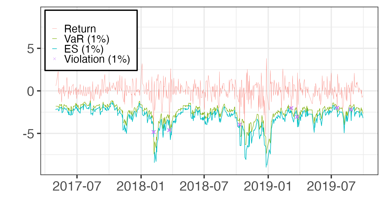
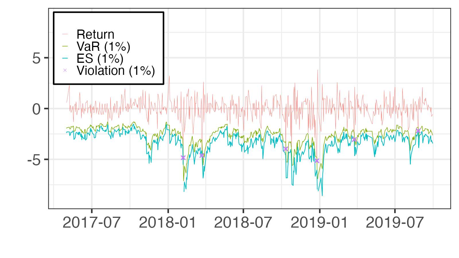
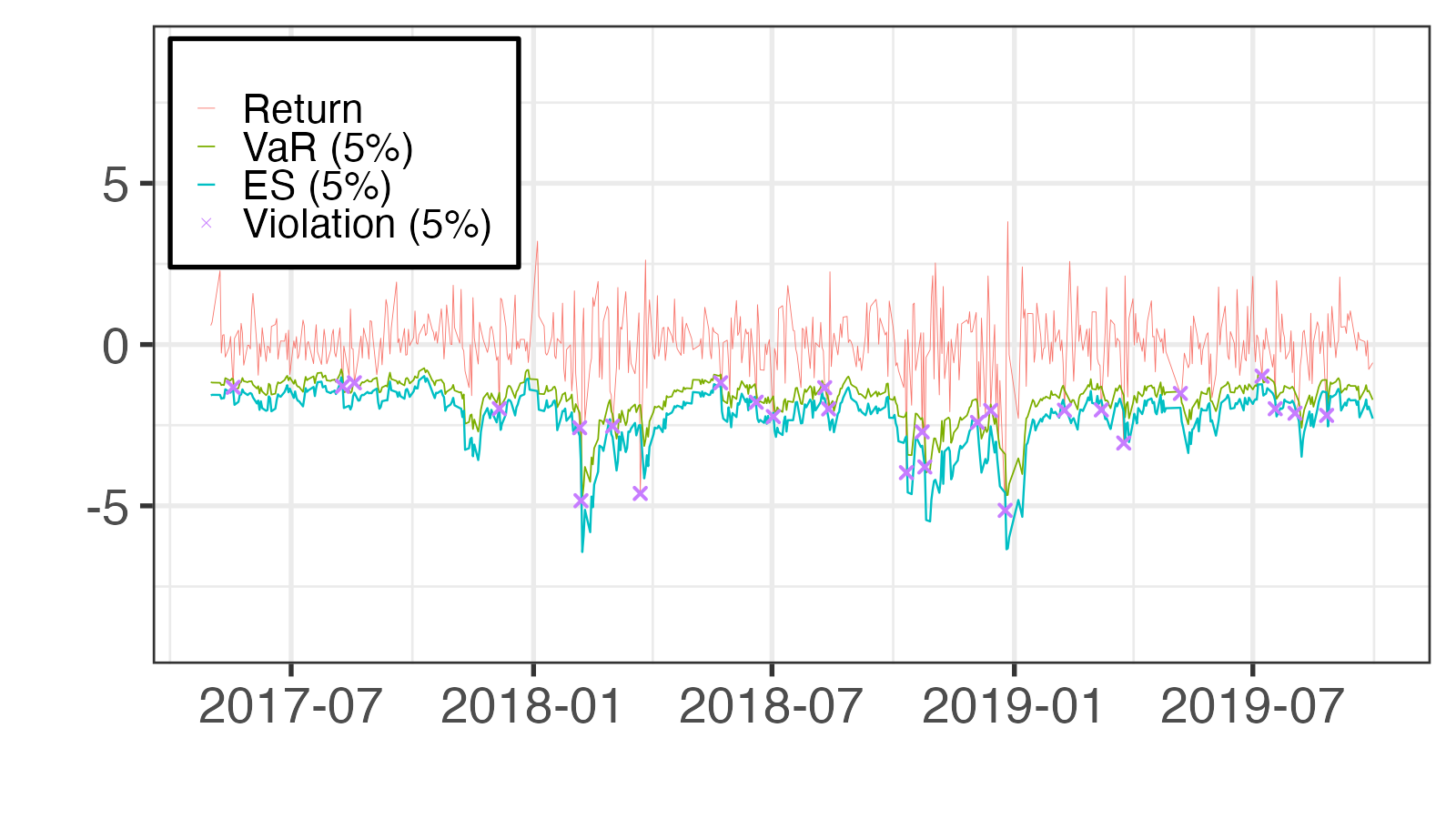
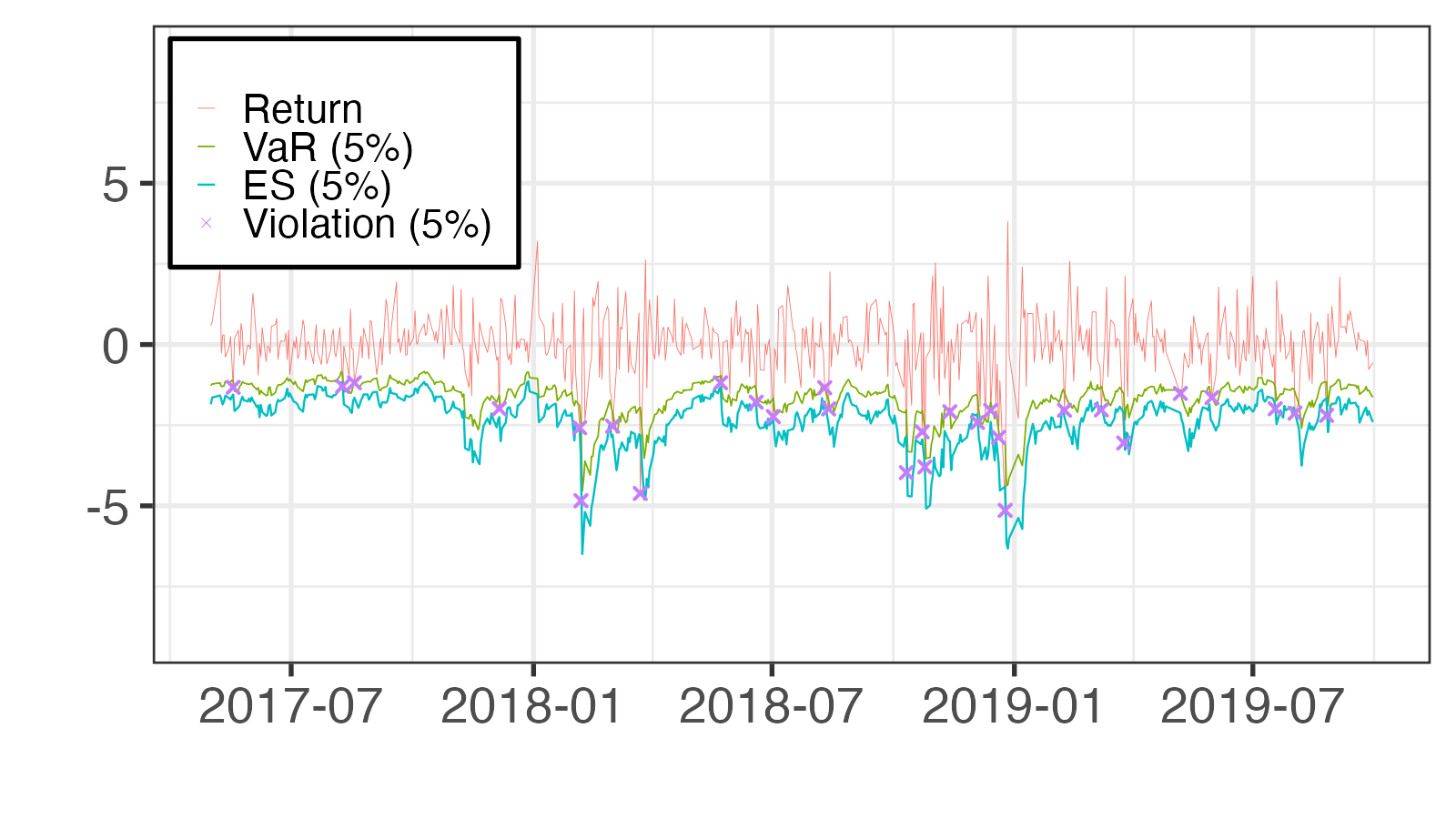
Figure 12: VaR and ES forecasts for N225: RSV-GH-ST model (left) vs. REGARCH-T model (right).

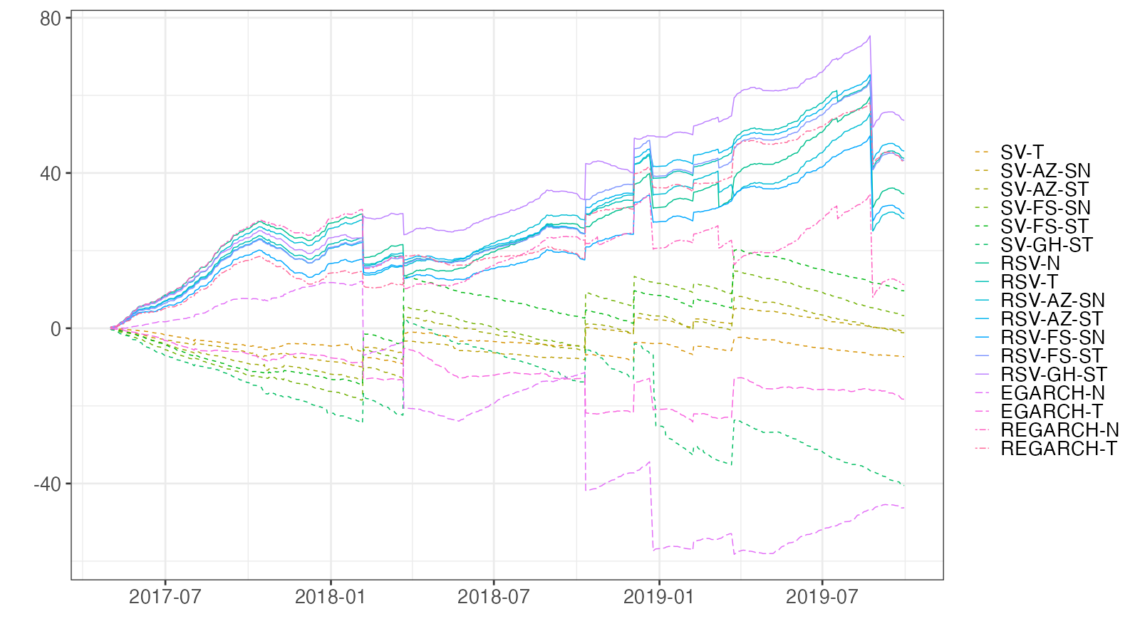
$\alpha=5\%$

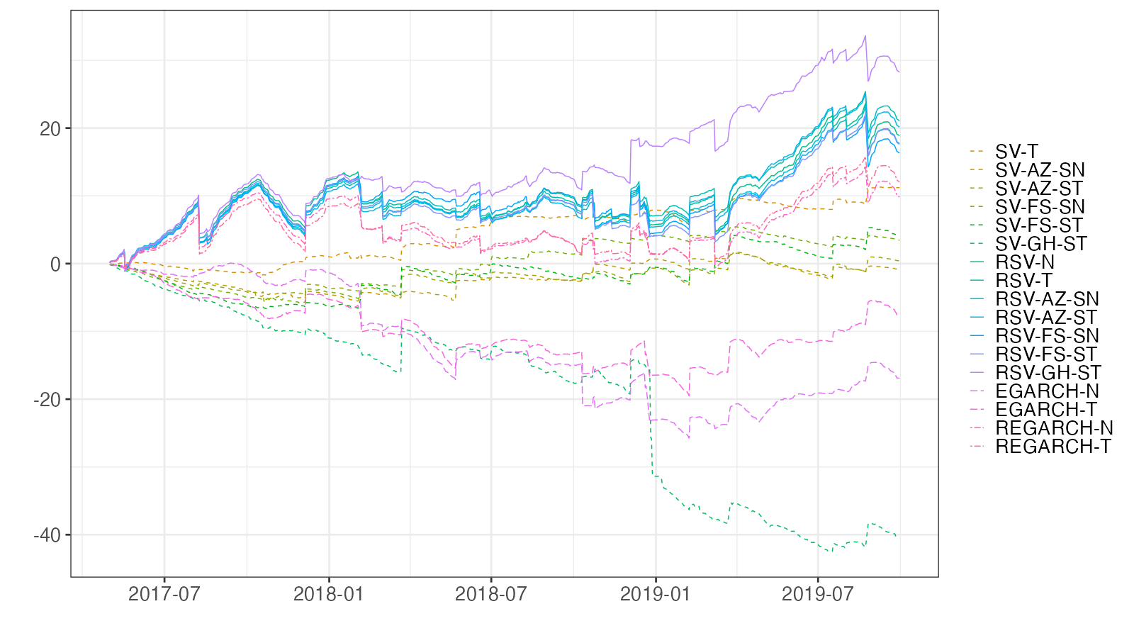
Figure 13: Cumulative loss differences (FZ0) in comparison to the SV-N model for N225

The prediction results for the N225 index are presented in Tables 11–13 and Figures 12–13. We observe that the VaR violations are closely aligned with the target rates across all models. For both significance levels $\alpha=1\%$ and $5\%$, the RSV-GH-ST model demonstrates the lowest FZ0 loss. Notably, the RSV and REGARCH models are included in the 90% MCS for both $\alpha=1\%$ and $5\%$. However, the SV and EGARCH models do not consistently meet this criterion.

The unconditional GW tests, summarized in the lower triangular elements of the tables, indicate that the RSV and REGARCH models frequently outperform the SV and EGARCH models, but not vice versa. Conversely, the conditional GW tests, presented in the upper triangular elements, suggest that the RSV models occasionally surpass the REGARCH models in performance. The CLDs reveal that for $\alpha=1\%$, the RSV and REGARCH models outperform the SV and EGARCH models throughout the entire period. Similarly, for $\alpha=5\%$, the RSV models maintain superiority almost throughout the entire period. Specifically, the RSV-GH-ST model surpasses other models in performance. These results underscore the efficacy of enhancing the RSV model by integrating a skewed-heavy tail distribution into the daily return for VaR and ES forecasts.

Table 11: Violation rates and FZ0 losses of VaR and ES forecasts for N225

	$\alpha=1\%$				$\alpha=5\%$
	$\hat{\alpha}$	FZ0	$p_{MCS}$		$\hat{\alpha}$	FZ0	$p_{MCS}$
SV-N	$1.02$	$1.2034$	$0.90^{**}$		$3.90$	$0.8163$	$0.42^{**}$
SV-T	$0.85$	$1.2158$	$0.53^{**}$		$3.39$	$0.7973$	$1.00^{**}$
SV-AZ-SN	$0.85$	$1.2047$	$0.89^{**}$		$3.56$	$0.8178$	$0.47^{**}$
SV-AZ-ST	$0.85$	$1.2053$	$0.94^{**}$		$3.56$	$0.8156$	$0.59^{**}$
SV-FS-SN	$0.85$	$1.1979$	$1.00^{**}$		$3.39$	$0.8105$	$0.83^{**}$
SV-FS-ST	$0.85$	$1.1870$	$1.00^{**}$		$3.39$	$0.8093$	$0.92^{**}$
SV-GH-ST	$0.68$	$1.2720$	$0.30^{**}$		$4.24$	$0.8846$	$0.00^{\hskip 5.60002pt}$
RSV-N	$1.53$	$1.1447$	$1.00^{**}$		$5.08$	$0.7844$	$1.00^{**}$
RSV-T	$1.36$	$1.1292$	$1.00^{**}$		$5.08$	$0.7806$	$1.00^{**}$
RSV-AZ-SN	$1.36$	$1.1555$	$1.00^{**}$		$4.75$	$0.7863$	$1.00^{**}$
RSV-AZ-ST	$1.19$	$1.1260$	$1.00^{**}$		$4.75$	$0.7822$	$1.00^{**}$
RSV-FS-SN	$1.19$	$1.1533$	$1.00^{**}$		$5.25$	$0.7887$	$1.00^{**}$
RSV-FS-ST	$1.19$	$1.1301$	$1.00^{**}$		$5.25$	$0.7865$	$1.00^{**}$
RSV-GH-ST	$1.19$	$1.1126$	$1.00^{**}$		$4.58$	$0.7685$	$1.00^{**}$
EGARCH-N	$1.02$	$1.2818$	$0.60^{**}$		$3.73$	$0.8450$	$0.00^{\hskip 5.60002pt}$
EGARCH-T	$1.02$	$1.2344$	$0.27^{**}$		$3.73$	$0.8292$	$0.25^{*\hskip 2.79996pt}$
REGARCH-N	$1.69$	$1.1844$	$1.00^{**}$		$4.41$	$0.7997$	$1.00^{**}$
REGARCH-T	$1.02$	$1.1306$	$1.00^{**}$		$4.92$	$0.7959$	$1.00^{**}$
Note: Refer to Table 5 for additional details.

Table 12: Summary of GW tests on FZ0 loss of VaR and ES forecasts ($\alpha=1\%$) for N225

	SV-N	T	AZ-SN	AZ-ST	FS-SN	FS-ST	GH-ST	RSV-N	T	AZ-SN	AZ-ST	FS-SN	FS-ST	GH-ST	EG-N	T	REG-N	T
SV-N		$\hskip 3.49998pt\hskip 1.99997pt\hskip 1.99997pt1^{**}$	$\hskip 3.49998pt\hskip 1.99997pt\hskip 1.99997pt1^{\hskip 2.8pt}$	$\hskip 3.49998pt\hskip 1.99997pt\hskip 1.99997pt0^{\hskip 2.8pt}$	$\hskip 3.49998pt\hskip 1.99997pt99^{\hskip 2.8pt}$	$\hskip 3.49998pt\hskip 1.99997pt99^{\hskip 2.8pt}$	$\hskip 3.49998pt\hskip 1.99997pt\hskip 1.99997pt0^{\hskip 2.8pt}$	$\hskip 3.49998pt100^{\hskip 2.8pt}$	$\hskip 3.49998pt100^{\hskip 2.8pt}$	$\hskip 3.49998pt100^{\hskip 2.8pt}$	$\hskip 3.49998pt100^{\hskip 2.8pt}$	$\hskip 3.49998pt100^{\hskip 2.8pt}$	$\hskip 3.49998pt100^{\hskip 2.8pt}$	$\hskip 3.49998pt100^{\hskip 2.8pt}$	$\hskip 3.49998pt\hskip 1.99997pt\hskip 1.99997pt1^{\hskip 2.8pt}$	$\hskip 3.49998pt\hskip 1.99997pt\hskip 1.99997pt0^{\hskip 2.8pt}$	$\hskip 3.49998pt100^{\hskip 2.8pt}$	$\hskip 3.49998pt100^{\hskip 2.8pt}$
SV-T	$\hskip 3.49998pt0.7^{\hskip 2.8pt}$		$\hskip 3.49998pt100^{\hskip 2.8pt}$	$\hskip 3.49998pt\hskip 1.99997pt99^{\hskip 2.8pt}$	$\hskip 3.49998pt\hskip 1.99997pt99^{\hskip 2.8pt}$	$\hskip 3.49998pt\hskip 1.99997pt99^{\hskip 2.8pt}$	$\hskip 3.49998pt\hskip 1.99997pt\hskip 1.99997pt0^{\hskip 2.8pt}$	$\hskip 3.49998pt100^{\hskip 2.8pt}$	$\hskip 3.49998pt100^{\hskip 2.8pt}$	$\hskip 3.49998pt100^{\hskip 2.8pt}$	$\hskip 3.49998pt100^{\hskip 2.8pt}$	$\hskip 3.49998pt100^{\hskip 2.8pt}$	$\hskip 3.49998pt100^{\hskip 2.8pt}$	$\hskip 3.49998pt100^{\hskip 2.8pt}$	$\hskip 3.49998pt\hskip 1.99997pt\hskip 1.99997pt1^{\hskip 2.8pt}$	$\hskip 3.49998pt\hskip 1.99997pt\hskip 1.99997pt0^{\hskip 2.8pt}$	$\hskip 3.49998pt100^{\hskip 2.8pt}$	$\hskip 3.49998pt100^{\hskip 2.8pt}$
SV-AZ-SN	$\hskip 3.49998pt0.1^{\hskip 2.8pt}$	$-0.5^{\hskip 2.8pt}$		$\hskip 3.49998pt\hskip 1.99997pt\hskip 1.99997pt1^{\hskip 2.8pt}$	$\hskip 3.49998pt\hskip 1.99997pt99^{\hskip 2.8pt}$	$\hskip 3.49998pt\hskip 1.99997pt99^{\hskip 2.8pt}$	$\hskip 3.49998pt\hskip 1.99997pt\hskip 1.99997pt0^{**}$	$\hskip 3.49998pt100^{\hskip 2.8pt}$	$\hskip 3.49998pt100^{\hskip 2.8pt}$	$\hskip 3.49998pt100^{\hskip 2.8pt}$	$\hskip 3.49998pt100^{\hskip 2.8pt}$	$\hskip 3.49998pt100^{\hskip 2.8pt}$	$\hskip 3.49998pt100^{\hskip 2.8pt}$	$\hskip 3.49998pt100^{\hskip 2.8pt}$	$\hskip 3.49998pt\hskip 1.99997pt\hskip 1.99997pt1^{\hskip 2.8pt}$	$\hskip 3.49998pt\hskip 1.99997pt\hskip 1.99997pt1^{\hskip 2.8pt}$	$\hskip 3.49998pt100^{\hskip 2.8pt}$	$\hskip 3.49998pt\hskip 1.99997pt99^{\hskip 2.8pt}$
SV-AZ-ST	$\hskip 3.49998pt0.1^{\hskip 2.8pt}$	$-0.4^{\hskip 2.8pt}$	$\hskip 3.49998pt0.0^{\hskip 2.8pt}$		$\hskip 3.49998pt\hskip 1.99997pt99^{\hskip 2.8pt}$	$\hskip 3.49998pt\hskip 1.99997pt99^{\hskip 2.8pt}$	$\hskip 3.49998pt\hskip 1.99997pt\hskip 1.99997pt0^{*\hskip 1.39998pt}$	$\hskip 3.49998pt100^{\hskip 2.8pt}$	$\hskip 3.49998pt100^{\hskip 2.8pt}$	$\hskip 3.49998pt100^{\hskip 2.8pt}$	$\hskip 3.49998pt100^{\hskip 2.8pt}$	$\hskip 3.49998pt100^{\hskip 2.8pt}$	$\hskip 3.49998pt100^{\hskip 2.8pt}$	$\hskip 3.49998pt100^{\hskip 2.8pt}$	$\hskip 3.49998pt\hskip 1.99997pt\hskip 1.99997pt1^{\hskip 2.8pt}$	$\hskip 3.49998pt\hskip 1.99997pt\hskip 1.99997pt1^{\hskip 2.8pt}$	$\hskip 3.49998pt100^{\hskip 2.8pt}$	$\hskip 3.49998pt\hskip 1.99997pt99^{\hskip 2.8pt}$
SV-FS-SN	$-0.1^{\hskip 2.8pt}$	$-0.5^{\hskip 2.8pt}$	$-0.3^{\hskip 2.8pt}$	$-0.3^{\hskip 2.8pt}$		$\hskip 3.49998pt100^{\hskip 2.8pt}$	$\hskip 3.49998pt\hskip 1.99997pt\hskip 1.99997pt0^{**}$	$\hskip 3.49998pt100^{\hskip 2.8pt}$	$\hskip 3.49998pt100^{\hskip 2.8pt}$	$\hskip 3.49998pt100^{\hskip 2.8pt}$	$\hskip 3.49998pt100^{\hskip 2.8pt}$	$\hskip 3.49998pt100^{\hskip 2.8pt}$	$\hskip 3.49998pt100^{\hskip 2.8pt}$	$\hskip 3.49998pt100^{\hskip 2.8pt}$	$\hskip 3.49998pt\hskip 1.99997pt\hskip 1.99997pt1^{\hskip 2.8pt}$	$\hskip 3.49998pt\hskip 1.99997pt\hskip 1.99997pt1^{\hskip 2.8pt}$	$\hskip 3.49998pt100^{\hskip 2.8pt}$	$\hskip 3.49998pt\hskip 1.99997pt99^{\hskip 2.8pt}$
SV-FS-ST	$-0.3^{\hskip 2.8pt}$	$-0.8^{\hskip 2.8pt}$	$-0.5^{\hskip 2.8pt}$	$-0.8^{\hskip 2.8pt}$	$-0.4^{\hskip 2.8pt}$		$\hskip 3.49998pt\hskip 1.99997pt\hskip 1.99997pt0^{**}$	$\hskip 3.49998pt100^{\hskip 2.8pt}$	$\hskip 3.49998pt100^{\hskip 2.8pt}$	$\hskip 3.49998pt100^{\hskip 2.8pt}$	$\hskip 3.49998pt100^{\hskip 2.8pt}$	$\hskip 3.49998pt100^{\hskip 2.8pt}$	$\hskip 3.49998pt100^{\hskip 2.8pt}$	$\hskip 3.49998pt100^{\hskip 2.8pt}$	$\hskip 3.49998pt\hskip 1.99997pt\hskip 1.99997pt1^{\hskip 2.8pt}$	$\hskip 3.49998pt\hskip 1.99997pt\hskip 1.99997pt1^{\hskip 2.8pt}$	$\hskip 3.49998pt\hskip 1.99997pt77^{\hskip 2.8pt}$	$\hskip 3.49998pt\hskip 1.99997pt99^{\hskip 2.8pt}$
SV-GH-ST	$\hskip 3.49998pt1.1^{\hskip 2.8pt}$	$\hskip 3.49998pt1.1^{\hskip 2.8pt}$	$\hskip 3.49998pt1.3^{\hskip 2.8pt}$	$\hskip 3.49998pt1.8^{\hskip 2.8pt}$	$\hskip 3.49998pt1.9^{\hskip 2.8pt}$	$\hskip 3.49998pt2.3^{*\hskip 1.39998pt}$		$\hskip 3.49998pt100^{\hskip 2.8pt}$	$\hskip 3.49998pt100^{\hskip 2.8pt}$	$\hskip 3.49998pt100^{\hskip 2.8pt}$	$\hskip 3.49998pt100^{\hskip 2.8pt}$	$\hskip 3.49998pt100^{\hskip 2.8pt}$	$\hskip 3.49998pt100^{\hskip 2.8pt}$	$\hskip 3.49998pt100^{*\hskip 1.39998pt}$	$\hskip 3.49998pt\hskip 1.99997pt\hskip 1.99997pt1^{\hskip 2.8pt}$	$\hskip 3.49998pt\hskip 1.99997pt94^{\hskip 2.8pt}$	$\hskip 3.49998pt\hskip 1.99997pt99^{\hskip 2.8pt}$	$\hskip 3.49998pt\hskip 1.99997pt99^{*\hskip 1.39998pt}$
RSV-N	$-1.0^{\hskip 2.8pt}$	$-1.2^{\hskip 2.8pt}$	$-1.0^{\hskip 2.8pt}$	$-0.9^{\hskip 2.8pt}$	$-0.7^{\hskip 2.8pt}$	$-0.5^{\hskip 2.8pt}$	$-1.5^{\hskip 2.8pt}$		$\hskip 3.49998pt\hskip 1.99997pt99^{\hskip 2.8pt}$	$\hskip 3.49998pt\hskip 1.99997pt\hskip 1.99997pt0^{*\hskip 1.39998pt}$	$\hskip 3.49998pt\hskip 1.99997pt99^{\hskip 2.8pt}$	$\hskip 3.49998pt\hskip 1.99997pt\hskip 1.99997pt0^{\hskip 2.8pt}$	$\hskip 3.49998pt\hskip 1.99997pt99^{\hskip 2.8pt}$	$\hskip 3.49998pt\hskip 1.99997pt99^{\hskip 2.8pt}$	$\hskip 3.49998pt\hskip 1.99997pt\hskip 1.99997pt0^{\hskip 2.8pt}$	$\hskip 3.49998pt\hskip 1.99997pt\hskip 1.99997pt0^{\hskip 2.8pt}$	$\hskip 3.49998pt\hskip 1.99997pt\hskip 1.99997pt0^{\hskip 2.8pt}$	$\hskip 3.49998pt\hskip 1.99997pt98^{\hskip 2.8pt}$
RSV-T	$-1.6^{\hskip 2.8pt}$	$-1.9^{\hskip 2.8pt}$	$-1.6^{\hskip 2.8pt}$	$-1.4^{\hskip 2.8pt}$	$-1.1^{\hskip 2.8pt}$	$-0.9^{\hskip 2.8pt}$	$-2.0^{*\hskip 1.39998pt}$	$-0.7^{\hskip 2.8pt}$		$\hskip 3.49998pt\hskip 1.99997pt\hskip 1.99997pt1^{*\hskip 1.39998pt}$	$\hskip 3.49998pt100^{\hskip 2.8pt}$	$\hskip 3.49998pt\hskip 1.99997pt\hskip 1.99997pt0^{\hskip 2.8pt}$	$\hskip 3.49998pt\hskip 1.99997pt\hskip 1.99997pt1^{\hskip 2.8pt}$	$\hskip 3.49998pt\hskip 1.99997pt99^{\hskip 2.8pt}$	$\hskip 3.49998pt\hskip 1.99997pt\hskip 1.99997pt0^{\hskip 2.8pt}$	$\hskip 3.49998pt\hskip 1.99997pt\hskip 1.99997pt0^{\hskip 2.8pt}$	$\hskip 3.49998pt\hskip 1.99997pt\hskip 1.99997pt1^{*\hskip 1.39998pt}$	$\hskip 3.49998pt\hskip 1.99997pt11^{\hskip 2.8pt}$
RSV-AZ-SN	$-0.8^{\hskip 2.8pt}$	$-1.0^{\hskip 2.8pt}$	$-0.8^{\hskip 2.8pt}$	$-0.7^{\hskip 2.8pt}$	$-0.5^{\hskip 2.8pt}$	$-0.4^{\hskip 2.8pt}$	$-1.4^{\hskip 2.8pt}$	$\hskip 3.49998pt0.6^{\hskip 2.8pt}$	$\hskip 3.49998pt1.1^{\hskip 2.8pt}$		$\hskip 3.49998pt\hskip 1.99997pt99^{*\hskip 1.39998pt}$	$\hskip 3.49998pt\hskip 1.99997pt98^{\hskip 2.8pt}$	$\hskip 3.49998pt\hskip 1.99997pt99^{*\hskip 1.39998pt}$	$\hskip 3.49998pt\hskip 1.99997pt99^{\hskip 2.8pt}$	$\hskip 3.49998pt\hskip 1.99997pt\hskip 1.99997pt0^{\hskip 2.8pt}$	$\hskip 3.49998pt\hskip 1.99997pt\hskip 1.99997pt0^{\hskip 2.8pt}$	$\hskip 3.49998pt\hskip 1.99997pt\hskip 1.99997pt1^{\hskip 2.8pt}$	$\hskip 3.49998pt\hskip 1.99997pt99^{\hskip 2.8pt}$
RSV-AZ-ST	$-1.7^{\hskip 2.8pt}$	$-2.0^{*\hskip 1.39998pt}$	$-1.7^{\hskip 2.8pt}$	$-1.6^{\hskip 2.8pt}$	$-1.2^{\hskip 2.8pt}$	$-1.0^{\hskip 2.8pt}$	$-2.2^{*\hskip 1.39998pt}$	$-0.7^{\hskip 2.8pt}$	$-0.3^{\hskip 2.8pt}$	$-1.3^{\hskip 2.8pt}$		$\hskip 3.49998pt\hskip 1.99997pt\hskip 1.99997pt0^{*\hskip 1.39998pt}$	$\hskip 3.49998pt\hskip 1.99997pt\hskip 1.99997pt1^{\hskip 2.8pt}$	$\hskip 3.49998pt\hskip 1.99997pt99^{\hskip 2.8pt}$	$\hskip 3.49998pt\hskip 1.99997pt\hskip 1.99997pt1^{\hskip 2.8pt}$	$\hskip 3.49998pt\hskip 1.99997pt\hskip 1.99997pt0^{\hskip 2.8pt}$	$\hskip 3.49998pt\hskip 1.99997pt\hskip 1.99997pt1^{*\hskip 1.39998pt}$	$\hskip 3.49998pt\hskip 1.99997pt\hskip 1.99997pt0^{\hskip 2.8pt}$
RSV-FS-SN	$-1.2^{\hskip 2.8pt}$	$-1.4^{\hskip 2.8pt}$	$-1.1^{\hskip 2.8pt}$	$-1.0^{\hskip 2.8pt}$	$-0.8^{\hskip 2.8pt}$	$-0.5^{\hskip 2.8pt}$	$-1.7^{\hskip 2.8pt}$	$\hskip 3.49998pt0.4^{\hskip 2.8pt}$	$\hskip 3.49998pt2.5^{*\hskip 1.39998pt}$	$-0.1^{\hskip 2.8pt}$	$\hskip 3.49998pt1.9^{\hskip 2.8pt}$		$\hskip 3.49998pt100^{\hskip 2.8pt}$	$\hskip 3.49998pt\hskip 1.99997pt99^{\hskip 2.8pt}$	$\hskip 3.49998pt\hskip 1.99997pt\hskip 1.99997pt1^{\hskip 2.8pt}$	$\hskip 3.49998pt\hskip 1.99997pt\hskip 1.99997pt0^{\hskip 2.8pt}$	$\hskip 3.49998pt\hskip 1.99997pt\hskip 1.99997pt2^{\hskip 2.8pt}$	$\hskip 3.49998pt\hskip 1.99997pt99^{\hskip 2.8pt}$
RSV-FS-ST	$-1.5^{\hskip 2.8pt}$	$-1.7^{\hskip 2.8pt}$	$-1.6^{\hskip 2.8pt}$	$-1.4^{\hskip 2.8pt}$	$-1.1^{\hskip 2.8pt}$	$-0.9^{\hskip 2.8pt}$	$-2.1^{*\hskip 1.39998pt}$	$-0.6^{\hskip 2.8pt}$	$\hskip 3.49998pt0.1^{\hskip 2.8pt}$	$-1.1^{\hskip 2.8pt}$	$\hskip 3.49998pt0.3^{\hskip 2.8pt}$	$-1.7^{\hskip 2.8pt}$		$\hskip 3.49998pt100^{\hskip 2.8pt}$	$\hskip 3.49998pt\hskip 1.99997pt\hskip 1.99997pt0^{\hskip 2.8pt}$	$\hskip 3.49998pt\hskip 1.99997pt\hskip 1.99997pt0^{\hskip 2.8pt}$	$\hskip 3.49998pt\hskip 1.99997pt\hskip 1.99997pt1^{*\hskip 1.39998pt}$	$\hskip 3.49998pt\hskip 1.99997pt72^{\hskip 2.8pt}$
RSV-GH-ST	$-1.9^{\hskip 2.8pt}$	$-2.0^{*\hskip 1.39998pt}$	$-2.1^{*\hskip 1.39998pt}$	$-1.7^{\hskip 2.8pt}$	$-1.6^{\hskip 2.8pt}$	$-1.2^{\hskip 2.8pt}$	$-2.2^{*\hskip 1.39998pt}$	$-0.9^{\hskip 2.8pt}$	$-0.7^{\hskip 2.8pt}$	$-1.1^{\hskip 2.8pt}$	$-0.5^{\hskip 2.8pt}$	$-1.8^{\hskip 2.8pt}$	$-0.7^{\hskip 2.8pt}$		$\hskip 3.49998pt\hskip 1.99997pt\hskip 1.99997pt1^{\hskip 2.8pt}$	$\hskip 3.49998pt\hskip 1.99997pt\hskip 1.99997pt0^{\hskip 2.8pt}$	$\hskip 3.49998pt\hskip 1.99997pt\hskip 1.99997pt1^{\hskip 2.8pt}$	$\hskip 3.49998pt\hskip 1.99997pt\hskip 1.99997pt0^{\hskip 2.8pt}$
EGARCH-N	$\hskip 3.49998pt1.0^{\hskip 2.8pt}$	$\hskip 3.49998pt0.8^{\hskip 2.8pt}$	$\hskip 3.49998pt0.8^{\hskip 2.8pt}$	$\hskip 3.49998pt0.8^{\hskip 2.8pt}$	$\hskip 3.49998pt0.7^{\hskip 2.8pt}$	$\hskip 3.49998pt0.9^{\hskip 2.8pt}$	$\hskip 3.49998pt0.1^{\hskip 2.8pt}$	$\hskip 3.49998pt1.7^{\hskip 2.8pt}$	$\hskip 3.49998pt1.8^{\hskip 2.8pt}$	$\hskip 3.49998pt1.6^{\hskip 2.8pt}$	$\hskip 3.49998pt1.8^{\hskip 2.8pt}$	$\hskip 3.49998pt1.6^{\hskip 2.8pt}$	$\hskip 3.49998pt1.7^{\hskip 2.8pt}$	$\hskip 3.49998pt1.7^{\hskip 2.8pt}$		$\hskip 3.49998pt\hskip 1.99997pt99^{\hskip 2.8pt}$	$\hskip 3.49998pt100^{\hskip 2.8pt}$	$\hskip 3.49998pt\hskip 1.99997pt99^{\hskip 2.8pt}$
EGARCH-T	$\hskip 3.49998pt0.9^{\hskip 2.8pt}$	$\hskip 3.49998pt0.8^{\hskip 2.8pt}$	$\hskip 3.49998pt0.8^{\hskip 2.8pt}$	$\hskip 3.49998pt0.8^{\hskip 2.8pt}$	$\hskip 3.49998pt0.7^{\hskip 2.8pt}$	$\hskip 3.49998pt1.2^{\hskip 2.8pt}$	$-0.7^{\hskip 2.8pt}$	$\hskip 3.49998pt1.5^{\hskip 2.8pt}$	$\hskip 3.49998pt2.1^{*\hskip 1.39998pt}$	$\hskip 3.49998pt1.3^{\hskip 2.8pt}$	$\hskip 3.49998pt2.2^{*\hskip 1.39998pt}$	$\hskip 3.49998pt1.7^{\hskip 2.8pt}$	$\hskip 3.49998pt2.0^{*\hskip 1.39998pt}$	$\hskip 3.49998pt2.1^{*\hskip 1.39998pt}$	$-0.7^{\hskip 2.8pt}$		$\hskip 3.49998pt100^{\hskip 2.8pt}$	$\hskip 3.49998pt100^{\hskip 2.8pt}$
REGARCH-N	$-0.3^{\hskip 2.8pt}$	$-0.5^{\hskip 2.8pt}$	$-0.3^{\hskip 2.8pt}$	$-0.3^{\hskip 2.8pt}$	$-0.2^{\hskip 2.8pt}$	$0.0^{\hskip 2.8pt}$	$-1.0^{\hskip 2.8pt}$	$\hskip 3.49998pt1.7^{\hskip 2.8pt}$	$\hskip 3.49998pt1.7^{\hskip 2.8pt}$	$\hskip 3.49998pt1.7^{\hskip 2.8pt}$	$\hskip 3.49998pt1.7^{\hskip 2.8pt}$	$\hskip 3.49998pt1.0^{\hskip 2.8pt}$	$\hskip 3.49998pt1.7^{\hskip 2.8pt}$	$\hskip 3.49998pt1.5^{\hskip 2.8pt}$	$-1.4^{\hskip 2.8pt}$	$-0.8^{\hskip 2.8pt}$		$\hskip 3.49998pt\hskip 1.99997pt99^{*\hskip 1.39998pt}$
REGARCH-T	$-1.7^{\hskip 2.8pt}$	$-2.2^{*\hskip 1.39998pt}$	$-2.0^{*\hskip 1.39998pt}$	$-2.1^{*\hskip 1.39998pt}$	$-1.6^{\hskip 2.8pt}$	$-1.2^{\hskip 2.8pt}$	$-2.7^{**}$	$-0.3^{\hskip 2.8pt}$	$\hskip 3.49998pt0.1^{\hskip 2.8pt}$	$-0.6^{\hskip 2.8pt}$	$\hskip 3.49998pt0.2^{\hskip 2.8pt}$	$-0.9^{\hskip 2.8pt}$	$\hskip 3.49998pt0.0^{\hskip 2.8pt}$	$\hskip 3.49998pt0.6^{\hskip 2.8pt}$	$-1.6^{\hskip 2.8pt}$	$-2.4^{*\hskip 1.39998pt}$	$-1.0^{\hskip 2.8pt}$

Note: Refer to Table 4 for additional details.

Table 13: Summary of GW tests on FZ0 loss of VaR and ES forecasts ($\alpha=5\%$) for N225

	SV-N	T	AZ-SN	AZ-ST	FS-SN	FS-ST	GH-ST	RSV-N	T	AZ-SN	AZ-ST	FS-SN	FS-ST	GH-ST	EG-N	T	REG-N	T
SV-N		$\hskip 3.49998pt\hskip 1.99997pt99^{\hskip 2.8pt}$	$\hskip 3.49998pt\hskip 1.99997pt\hskip 1.99997pt5^{\hskip 2.8pt}$	$\hskip 3.49998pt\hskip 1.99997pt53^{\hskip 2.8pt}$	$\hskip 3.49998pt\hskip 1.99997pt97^{\hskip 2.8pt}$	$\hskip 3.49998pt100^{\hskip 2.8pt}$	$\hskip 3.49998pt\hskip 1.99997pt\hskip 1.99997pt1^{**}$	$\hskip 3.49998pt\hskip 1.99997pt99^{\hskip 2.8pt}$	$\hskip 3.49998pt100^{\hskip 2.8pt}$	$\hskip 3.49998pt\hskip 1.99997pt99^{\hskip 2.8pt}$	$\hskip 3.49998pt100^{\hskip 2.8pt}$	$\hskip 3.49998pt100^{\hskip 2.8pt}$	$\hskip 3.49998pt\hskip 1.99997pt99^{\hskip 2.8pt}$	$\hskip 3.49998pt100^{\hskip 2.8pt}$	$\hskip 3.49998pt\hskip 1.99997pt\hskip 1.99997pt1^{\hskip 2.8pt}$	$\hskip 3.49998pt\hskip 1.99997pt\hskip 1.99997pt2^{\hskip 2.8pt}$	$\hskip 3.49998pt\hskip 1.99997pt98^{\hskip 2.8pt}$	$\hskip 3.49998pt100^{\hskip 2.8pt}$
SV-T	$-2.0^{*\hskip 1.39998pt}$		$\hskip 3.49998pt\hskip 1.99997pt\hskip 1.99997pt0^{\hskip 2.8pt}$	$\hskip 3.49998pt\hskip 1.99997pt\hskip 1.99997pt1^{\hskip 2.8pt}$	$\hskip 3.49998pt\hskip 1.99997pt\hskip 1.99997pt1^{\hskip 2.8pt}$	$\hskip 3.49998pt\hskip 1.99997pt\hskip 1.99997pt3^{\hskip 2.8pt}$	$\hskip 3.49998pt\hskip 1.99997pt\hskip 1.99997pt0^{**}$	$\hskip 3.49998pt100^{\hskip 2.8pt}$	$\hskip 3.49998pt100^{\hskip 2.8pt}$	$\hskip 3.49998pt100^{\hskip 2.8pt}$	$\hskip 3.49998pt100^{\hskip 2.8pt}$	$\hskip 3.49998pt\hskip 1.99997pt99^{\hskip 2.8pt}$	$\hskip 3.49998pt100^{\hskip 2.8pt}$	$\hskip 3.49998pt\hskip 1.99997pt99^{\hskip 2.8pt}$	$\hskip 3.49998pt\hskip 1.99997pt\hskip 1.99997pt1^{*\hskip 1.39998pt}$	$\hskip 3.49998pt\hskip 1.99997pt\hskip 1.99997pt2^{\hskip 2.8pt}$	$\hskip 3.49998pt\hskip 1.99997pt15^{\hskip 2.8pt}$	$\hskip 3.49998pt\hskip 1.99997pt99^{\hskip 2.8pt}$
SV-AZ-SN	$\hskip 3.49998pt0.2^{\hskip 2.8pt}$	$\hskip 3.49998pt3.2^{**}$		$\hskip 3.49998pt\hskip 1.99997pt97^{\hskip 2.8pt}$	$\hskip 3.49998pt\hskip 1.99997pt97^{*\hskip 1.39998pt}$	$\hskip 3.49998pt\hskip 1.99997pt99^{\hskip 2.8pt}$	$\hskip 3.49998pt\hskip 1.99997pt\hskip 1.99997pt1^{**}$	$\hskip 3.49998pt\hskip 1.99997pt98^{\hskip 2.8pt}$	$\hskip 3.49998pt\hskip 1.99997pt99^{\hskip 2.8pt}$	$\hskip 3.49998pt\hskip 1.99997pt98^{\hskip 2.8pt}$	$\hskip 3.49998pt\hskip 1.99997pt98^{\hskip 2.8pt}$	$\hskip 3.49998pt100^{\hskip 2.8pt}$	$\hskip 3.49998pt\hskip 1.99997pt98^{\hskip 2.8pt}$	$\hskip 3.49998pt100^{\hskip 2.8pt}$	$\hskip 3.49998pt\hskip 1.99997pt\hskip 1.99997pt2^{\hskip 2.8pt}$	$\hskip 3.49998pt\hskip 1.99997pt\hskip 1.99997pt2^{\hskip 2.8pt}$	$\hskip 3.49998pt\hskip 1.99997pt97^{\hskip 2.8pt}$	$\hskip 3.49998pt\hskip 1.99997pt98^{\hskip 2.8pt}$
SV-AZ-ST	$-0.1^{\hskip 2.8pt}$	$\hskip 3.49998pt3.2^{**}$	$-0.3^{\hskip 2.8pt}$		$\hskip 3.49998pt\hskip 1.99997pt99^{\hskip 2.8pt}$	$\hskip 3.49998pt\hskip 1.99997pt86^{\hskip 2.8pt}$	$\hskip 3.49998pt\hskip 1.99997pt\hskip 1.99997pt0^{**}$	$\hskip 3.49998pt\hskip 1.99997pt99^{\hskip 2.8pt}$	$\hskip 3.49998pt100^{\hskip 2.8pt}$	$\hskip 3.49998pt\hskip 1.99997pt99^{\hskip 2.8pt}$	$\hskip 3.49998pt100^{\hskip 2.8pt}$	$\hskip 3.49998pt100^{\hskip 2.8pt}$	$\hskip 3.49998pt\hskip 1.99997pt99^{\hskip 2.8pt}$	$\hskip 3.49998pt100^{\hskip 2.8pt}$	$\hskip 3.49998pt\hskip 1.99997pt\hskip 1.99997pt1^{\hskip 2.8pt}$	$\hskip 3.49998pt\hskip 1.99997pt\hskip 1.99997pt2^{\hskip 2.8pt}$	$\hskip 3.49998pt\hskip 1.99997pt97^{\hskip 2.8pt}$	$\hskip 3.49998pt100^{\hskip 2.8pt}$
SV-FS-SN	$-0.6^{\hskip 2.8pt}$	$\hskip 3.49998pt1.4^{\hskip 2.8pt}$	$-1.1^{\hskip 2.8pt}$	$-0.7^{\hskip 2.8pt}$		$\hskip 3.49998pt\hskip 1.99997pt99^{\hskip 2.8pt}$	$\hskip 3.49998pt\hskip 1.99997pt\hskip 1.99997pt1^{**}$	$\hskip 3.49998pt\hskip 1.99997pt97^{\hskip 2.8pt}$	$\hskip 3.49998pt\hskip 1.99997pt98^{\hskip 2.8pt}$	$\hskip 3.49998pt\hskip 1.99997pt97^{\hskip 2.8pt}$	$\hskip 3.49998pt\hskip 1.99997pt97^{\hskip 2.8pt}$	$\hskip 3.49998pt\hskip 1.99997pt99^{\hskip 2.8pt}$	$\hskip 3.49998pt\hskip 1.99997pt97^{\hskip 2.8pt}$	$\hskip 3.49998pt100^{\hskip 2.8pt}$	$\hskip 3.49998pt\hskip 1.99997pt\hskip 1.99997pt1^{\hskip 2.8pt}$	$\hskip 3.49998pt\hskip 1.99997pt\hskip 1.99997pt1^{\hskip 2.8pt}$	$\hskip 3.49998pt\hskip 1.99997pt96^{\hskip 2.8pt}$	$\hskip 3.49998pt\hskip 1.99997pt97^{\hskip 2.8pt}$
SV-FS-ST	$-0.5^{\hskip 2.8pt}$	$\hskip 3.49998pt1.3^{\hskip 2.8pt}$	$-0.8^{\hskip 2.8pt}$	$-0.8^{\hskip 2.8pt}$	$-0.1^{\hskip 2.8pt}$		$\hskip 3.49998pt\hskip 1.99997pt\hskip 1.99997pt1^{**}$	$\hskip 3.49998pt\hskip 1.99997pt97^{\hskip 2.8pt}$	$\hskip 3.49998pt\hskip 1.99997pt97^{\hskip 2.8pt}$	$\hskip 3.49998pt\hskip 1.99997pt97^{\hskip 2.8pt}$	$\hskip 3.49998pt\hskip 1.99997pt97^{\hskip 2.8pt}$	$\hskip 3.49998pt\hskip 1.99997pt97^{\hskip 2.8pt}$	$\hskip 3.49998pt\hskip 1.99997pt97^{\hskip 2.8pt}$	$\hskip 3.49998pt100^{\hskip 2.8pt}$	$\hskip 3.49998pt\hskip 1.99997pt\hskip 1.99997pt1^{\hskip 2.8pt}$	$\hskip 3.49998pt\hskip 1.99997pt\hskip 1.99997pt6^{\hskip 2.8pt}$	$\hskip 3.49998pt\hskip 1.99997pt94^{\hskip 2.8pt}$	$\hskip 3.49998pt\hskip 1.99997pt96^{\hskip 2.8pt}$
SV-GH-ST	$\hskip 3.49998pt2.2^{*\hskip 1.39998pt}$	$\hskip 3.49998pt3.0^{**}$	$\hskip 3.49998pt2.2^{*\hskip 1.39998pt}$	$\hskip 3.49998pt2.4^{*\hskip 1.39998pt}$	$\hskip 3.49998pt2.4^{*\hskip 1.39998pt}$	$\hskip 3.49998pt2.5^{*\hskip 1.39998pt}$		$\hskip 3.49998pt\hskip 1.99997pt99^{\hskip 2.8pt}$	$\hskip 3.49998pt\hskip 1.99997pt99^{\hskip 2.8pt}$	$\hskip 3.49998pt\hskip 1.99997pt99^{\hskip 2.8pt}$	$\hskip 3.49998pt\hskip 1.99997pt99^{\hskip 2.8pt}$	$\hskip 3.49998pt\hskip 1.99997pt99^{\hskip 2.8pt}$	$\hskip 3.49998pt\hskip 1.99997pt99^{\hskip 2.8pt}$	$\hskip 3.49998pt100^{*\hskip 1.39998pt}$	$\hskip 3.49998pt\hskip 1.99997pt96^{*\hskip 1.39998pt}$	$\hskip 3.49998pt\hskip 1.99997pt98^{*\hskip 1.39998pt}$	$\hskip 3.49998pt\hskip 1.99997pt99^{\hskip 2.8pt}$	$\hskip 3.49998pt\hskip 1.99997pt99^{\hskip 2.8pt}$
RSV-N	$-1.2^{\hskip 2.8pt}$	$-0.4^{\hskip 2.8pt}$	$-1.1^{\hskip 2.8pt}$	$-1.1^{\hskip 2.8pt}$	$-0.9^{\hskip 2.8pt}$	$-0.8^{\hskip 2.8pt}$	$-2.6^{**}$		$\hskip 3.49998pt\hskip 1.99997pt99^{\hskip 2.8pt}$	$\hskip 3.49998pt\hskip 1.99997pt\hskip 1.99997pt1^{\hskip 2.8pt}$	$\hskip 3.49998pt\hskip 1.99997pt98^{\hskip 2.8pt}$	$\hskip 3.49998pt\hskip 1.99997pt\hskip 1.99997pt2^{\hskip 2.8pt}$	$\hskip 3.49998pt\hskip 1.99997pt\hskip 1.99997pt3^{\hskip 2.8pt}$	$\hskip 3.49998pt\hskip 1.99997pt98^{\hskip 2.8pt}$	$\hskip 3.49998pt\hskip 1.99997pt\hskip 1.99997pt0^{\hskip 2.8pt}$	$\hskip 3.49998pt\hskip 1.99997pt\hskip 1.99997pt0^{\hskip 2.8pt}$	$\hskip 3.49998pt\hskip 1.99997pt\hskip 1.99997pt0^{**}$	$\hskip 3.49998pt\hskip 1.99997pt\hskip 1.99997pt0^{\hskip 2.8pt}$
RSV-T	$-1.4^{\hskip 2.8pt}$	$-0.6^{\hskip 2.8pt}$	$-1.4^{\hskip 2.8pt}$	$-1.3^{\hskip 2.8pt}$	$-1.1^{\hskip 2.8pt}$	$-0.9^{\hskip 2.8pt}$	$-2.9^{**}$	$-0.8^{\hskip 2.8pt}$		$\hskip 3.49998pt\hskip 1.99997pt\hskip 1.99997pt0^{*\hskip 1.39998pt}$	$\hskip 3.49998pt\hskip 1.99997pt\hskip 1.99997pt0^{\hskip 2.8pt}$	$\hskip 3.49998pt\hskip 1.99997pt\hskip 1.99997pt0^{\hskip 2.8pt}$	$\hskip 3.49998pt\hskip 1.99997pt\hskip 1.99997pt1^{\hskip 2.8pt}$	$\hskip 3.49998pt\hskip 1.99997pt98^{\hskip 2.8pt}$	$\hskip 3.49998pt\hskip 1.99997pt\hskip 1.99997pt0^{\hskip 2.8pt}$	$\hskip 3.49998pt\hskip 1.99997pt\hskip 1.99997pt0^{\hskip 2.8pt}$	$\hskip 3.49998pt\hskip 1.99997pt\hskip 1.99997pt0^{**}$	$\hskip 3.49998pt\hskip 1.99997pt\hskip 1.99997pt0^{\hskip 2.8pt}$
RSV-AZ-SN	$-1.2^{\hskip 2.8pt}$	$-0.4^{\hskip 2.8pt}$	$-1.1^{\hskip 2.8pt}$	$-1.0^{\hskip 2.8pt}$	$-0.8^{\hskip 2.8pt}$	$-0.7^{\hskip 2.8pt}$	$-2.6^{**}$	$\hskip 3.49998pt0.5^{\hskip 2.8pt}$	$\hskip 3.49998pt1.4^{\hskip 2.8pt}$		$\hskip 3.49998pt\hskip 1.99997pt99^{\hskip 2.8pt}$	$\hskip 3.49998pt\hskip 1.99997pt\hskip 1.99997pt2^{\hskip 2.8pt}$	$\hskip 3.49998pt\hskip 1.99997pt31^{\hskip 2.8pt}$	$\hskip 3.49998pt\hskip 1.99997pt99^{\hskip 2.8pt}$	$\hskip 3.49998pt\hskip 1.99997pt\hskip 1.99997pt0^{\hskip 2.8pt}$	$\hskip 3.49998pt\hskip 1.99997pt\hskip 1.99997pt0^{\hskip 2.8pt}$	$\hskip 3.49998pt\hskip 1.99997pt\hskip 1.99997pt0^{*\hskip 1.39998pt}$	$\hskip 3.49998pt\hskip 1.99997pt\hskip 1.99997pt0^{\hskip 2.8pt}$
RSV-AZ-ST	$-1.4^{\hskip 2.8pt}$	$-0.6^{\hskip 2.8pt}$	$-1.3^{\hskip 2.8pt}$	$-1.2^{\hskip 2.8pt}$	$-1.0^{\hskip 2.8pt}$	$-0.9^{\hskip 2.8pt}$	$-2.8^{**}$	$-0.4^{\hskip 2.8pt}$	$\hskip 3.49998pt0.5^{\hskip 2.8pt}$	$-1.0^{\hskip 2.8pt}$		$\hskip 3.49998pt\hskip 1.99997pt\hskip 1.99997pt0^{*\hskip 1.39998pt}$	$\hskip 3.49998pt\hskip 1.99997pt\hskip 1.99997pt1^{\hskip 2.8pt}$	$\hskip 3.49998pt\hskip 1.99997pt98^{\hskip 2.8pt}$	$\hskip 3.49998pt\hskip 1.99997pt\hskip 1.99997pt0^{\hskip 2.8pt}$	$\hskip 3.49998pt\hskip 1.99997pt\hskip 1.99997pt0^{\hskip 2.8pt}$	$\hskip 3.49998pt\hskip 1.99997pt\hskip 1.99997pt0^{**}$	$\hskip 3.49998pt\hskip 1.99997pt\hskip 1.99997pt0^{\hskip 2.8pt}$
RSV-FS-SN	$-1.1^{\hskip 2.8pt}$	$-0.3^{\hskip 2.8pt}$	$-1.0^{\hskip 2.8pt}$	$-0.9^{\hskip 2.8pt}$	$-0.7^{\hskip 2.8pt}$	$-0.6^{\hskip 2.8pt}$	$-2.6^{**}$	$\hskip 3.49998pt0.9^{\hskip 2.8pt}$	$\hskip 3.49998pt1.5^{\hskip 2.8pt}$	$\hskip 3.49998pt0.6^{\hskip 2.8pt}$	$\hskip 3.49998pt1.1^{\hskip 2.8pt}$		$\hskip 3.49998pt\hskip 1.99997pt99^{\hskip 2.8pt}$	$\hskip 3.49998pt100^{\hskip 2.8pt}$	$\hskip 3.49998pt\hskip 1.99997pt\hskip 1.99997pt0^{\hskip 2.8pt}$	$\hskip 3.49998pt\hskip 1.99997pt\hskip 1.99997pt0^{\hskip 2.8pt}$	$\hskip 3.49998pt\hskip 1.99997pt\hskip 1.99997pt2^{**}$	$\hskip 3.49998pt\hskip 1.99997pt\hskip 1.99997pt0^{\hskip 2.8pt}$
RSV-FS-ST	$-1.2^{\hskip 2.8pt}$	$-0.4^{\hskip 2.8pt}$	$-1.1^{\hskip 2.8pt}$	$-1.0^{\hskip 2.8pt}$	$-0.8^{\hskip 2.8pt}$	$-0.7^{\hskip 2.8pt}$	$-2.7^{**}$	$\hskip 3.49998pt0.6^{\hskip 2.8pt}$	$\hskip 3.49998pt1.5^{\hskip 2.8pt}$	$\hskip 3.49998pt0.1^{\hskip 2.8pt}$	$\hskip 3.49998pt1.0^{\hskip 2.8pt}$	$-0.4^{\hskip 2.8pt}$		$\hskip 3.49998pt\hskip 1.99997pt98^{\hskip 2.8pt}$	$\hskip 3.49998pt\hskip 1.99997pt\hskip 1.99997pt0^{\hskip 2.8pt}$	$\hskip 3.49998pt\hskip 1.99997pt\hskip 1.99997pt0^{\hskip 2.8pt}$	$\hskip 3.49998pt\hskip 1.99997pt\hskip 1.99997pt0^{**}$	$\hskip 3.49998pt\hskip 1.99997pt\hskip 1.99997pt0^{\hskip 2.8pt}$
RSV-GH-ST	$-1.9^{\hskip 2.8pt}$	$-1.1^{\hskip 2.8pt}$	$-1.9^{\hskip 2.8pt}$	$-1.7^{\hskip 2.8pt}$	$-1.6^{\hskip 2.8pt}$	$-1.4^{\hskip 2.8pt}$	$-3.1^{**}$	$-1.2^{\hskip 2.8pt}$	$-1.1^{\hskip 2.8pt}$	$-1.4^{\hskip 2.8pt}$	$-1.2^{\hskip 2.8pt}$	$-1.6^{\hskip 2.8pt}$	$-1.4^{\hskip 2.8pt}$		$\hskip 3.49998pt\hskip 1.99997pt\hskip 1.99997pt0^{\hskip 2.8pt}$	$\hskip 3.49998pt\hskip 1.99997pt\hskip 1.99997pt0^{\hskip 2.8pt}$	$\hskip 3.49998pt\hskip 1.99997pt\hskip 1.99997pt2^{*\hskip 1.39998pt}$	$\hskip 3.49998pt\hskip 1.99997pt\hskip 1.99997pt1^{\hskip 2.8pt}$
EGARCH-N	$\hskip 3.49998pt1.2^{\hskip 2.8pt}$	$\hskip 3.49998pt2.2^{*\hskip 1.39998pt}$	$\hskip 3.49998pt1.1^{\hskip 2.8pt}$	$\hskip 3.49998pt1.2^{\hskip 2.8pt}$	$\hskip 3.49998pt1.3^{\hskip 2.8pt}$	$\hskip 3.49998pt1.4^{\hskip 2.8pt}$	$-1.3^{\hskip 2.8pt}$	$\hskip 3.49998pt2.1^{*\hskip 1.39998pt}$	$\hskip 3.49998pt2.3^{*\hskip 1.39998pt}$	$\hskip 3.49998pt2.1^{*\hskip 1.39998pt}$	$\hskip 3.49998pt2.2^{*\hskip 1.39998pt}$	$\hskip 3.49998pt2.0^{*\hskip 1.39998pt}$	$\hskip 3.49998pt2.1^{*\hskip 1.39998pt}$	$\hskip 3.49998pt2.4^{*\hskip 1.39998pt}$		$\hskip 3.49998pt100^{\hskip 2.8pt}$	$\hskip 3.49998pt100^{\hskip 2.8pt}$	$\hskip 3.49998pt100^{\hskip 2.8pt}$
EGARCH-T	$\hskip 3.49998pt0.6^{\hskip 2.8pt}$	$\hskip 3.49998pt2.0^{*\hskip 1.39998pt}$	$\hskip 3.49998pt0.6^{\hskip 2.8pt}$	$\hskip 3.49998pt0.8^{\hskip 2.8pt}$	$\hskip 3.49998pt0.9^{\hskip 2.8pt}$	$\hskip 3.49998pt1.1^{\hskip 2.8pt}$	$-2.0^{*\hskip 1.39998pt}$	$\hskip 3.49998pt1.5^{\hskip 2.8pt}$	$\hskip 3.49998pt1.8^{\hskip 2.8pt}$	$\hskip 3.49998pt1.5^{\hskip 2.8pt}$	$\hskip 3.49998pt1.7^{\hskip 2.8pt}$	$\hskip 3.49998pt1.4^{\hskip 2.8pt}$	$\hskip 3.49998pt1.5^{\hskip 2.8pt}$	$\hskip 3.49998pt2.0^{*\hskip 1.39998pt}$	$-1.5^{\hskip 2.8pt}$		$\hskip 3.49998pt100^{\hskip 2.8pt}$	$\hskip 3.49998pt100^{\hskip 2.8pt}$
REGARCH-N	$-0.7^{\hskip 2.8pt}$	$\hskip 3.49998pt0.1^{\hskip 2.8pt}$	$-0.7^{\hskip 2.8pt}$	$-0.6^{\hskip 2.8pt}$	$-0.4^{\hskip 2.8pt}$	$-0.3^{\hskip 2.8pt}$	$-2.4^{*\hskip 1.39998pt}$	$\hskip 3.49998pt2.1^{*\hskip 1.39998pt}$	$\hskip 3.49998pt3.2^{**}$	$\hskip 3.49998pt2.0^{*\hskip 1.39998pt}$	$\hskip 3.49998pt3.0^{**}$	$\hskip 3.49998pt1.3^{\hskip 2.8pt}$	$\hskip 3.49998pt2.1^{*\hskip 1.39998pt}$	$\hskip 3.49998pt2.4^{*\hskip 1.39998pt}$	$-1.8^{\hskip 2.8pt}$	$-1.2^{\hskip 2.8pt}$		$\hskip 3.49998pt\hskip 1.99997pt98^{\hskip 2.8pt}$
REGARCH-T	$-0.9^{\hskip 2.8pt}$	$-0.1^{\hskip 2.8pt}$	$-0.9^{\hskip 2.8pt}$	$-0.8^{\hskip 2.8pt}$	$-0.6^{\hskip 2.8pt}$	$-0.5^{\hskip 2.8pt}$	$-2.6^{**}$	$\hskip 3.49998pt1.3^{\hskip 2.8pt}$	$\hskip 3.49998pt2.6^{**}$	$\hskip 3.49998pt1.2^{\hskip 2.8pt}$	$\hskip 3.49998pt2.4^{*\hskip 1.39998pt}$	$\hskip 3.49998pt0.8^{\hskip 2.8pt}$	$\hskip 3.49998pt1.4^{\hskip 2.8pt}$	$\hskip 3.49998pt2.2^{*\hskip 1.39998pt}$	$-1.8^{\hskip 2.8pt}$	$-1.4^{\hskip 2.8pt}$	$-0.8^{\hskip 2.8pt}$

Note: Refer to Table 4 for additional details.

$\alpha=1\%$

References

- (1)
- Aas and Haff (2006) Aas, K. and Haff, I. H. (2006), ‘The generalized hyperbolic skew Student’s t-distribution’, Journal of Financial Econometrics 4(2), 275–309.
- Abanto-Valle et al. (2015) Abanto-Valle, C. A., Lachos, V. H. and Dey, D. K. (2015), ‘Bayesian Estimation of a Skew-Student-t Stochastic Volatility Model’, Methodology and Computing in Applied Probability 17(3), 721–738.
- Aït-sahalia and Mykland (2009) Aït-sahalia, Y. and Mykland, P. A. (2009), Estimating volatility in the presence of market microstructure noise: A review of the theory and practical considerations, in T. G. Andersen, R. A. Davis, J.-P. Kreiß and T. Mikosch, eds, ‘Handbook of Financial Time Series’, Springer-Verlag, Berlin, pp. 577–598.
- Aït-Sahalia et al. (2005) Aït-Sahalia, Y., Mykland, P. A. and Zhang, L. (2005), ‘How Often to Sample a Continuous-Time Process in the Presence of Market Microstructure Noise’, Review of Financial Studies 18(2), 351–416.
- Andersen and Benzoni (2009) Andersen, T. G. and Benzoni, L. (2009), Realized volatility, in T. G. Andersen, R. A. Davis, J.-P. Kreiß and T. Mikosch, eds, ‘Handbook of Financial Time Series’, Springer-Verlag, Berlin, pp. 555–575.
- Andersen et al. (2013) Andersen, T. G., Bollerslev, T., Christoffersen, P. F. and Diebold, F. X. (2013), Financial Risk Measurement for Financial Risk Management, in G. M. Constantinides, M. Harris and R. M. Stulz, eds, ‘Handbook of the Economics of Finance’, Vol. 2B, North Holland, Amsterdam, chapter 17, pp. 1127–1220.
- Andersen et al. (2003) Andersen, T. G., Bollerslev, T., Diebold, F. X. and Labys, P. (2003), ‘Modeling and forecasting realized volatility’, Econometrica 71(2), 579–625.
- Azzalini (1985) Azzalini, A. (1985), ‘A Class of Distributions which Includes the Normal Ones’, Scandinavian Journal of Statistics 12(2), 171–178.
- Azzalini and Capitanio (2003) Azzalini, A. and Capitanio, A. (2003), ‘Distributions generated by perturbation of symmetry with emphasis on a multivariate skew t-distribution’, Journal of the Royal Statistical Society B 65(2), 367–389.
- Bandi and Russell (2006) Bandi, F. M. and Russell, J. R. (2006), ‘Separating microstructure noise from volatility’, Journal of Financial Economics 79(3), 367–389.
- Bandi and Russell (2008) Bandi, F. M. and Russell, J. R. (2008), ‘Microstructure noise, realized volatility, and optimal sampling’, Review of Economic Studies 75(2), 655–692.
- Barndorff-Nielsen et al. (2008) Barndorff-Nielsen, O. E., Hansen, P. R., Lunde, A. and Shephard, N. (2008), ‘Designing realized kernels to measure the ex post variation of equity prices in the presence of noise’, Econometrica 76(6), 1481–1536.
- Barndorff-Nielsen et al. (2009) Barndorff-Nielsen, O. E., Hansen, P. R., Lunde, A. and Shephard, N. (2009), ‘Realized kernels in practice: Trades and quotes’, Econometrics Journal 12(3), C1–C32.
- Beran (1994) Beran, J. (1994), Statistics for Long-Memory Processes, 1st edition edn, Chapman \& Hall.
- Bollerslev (1986) Bollerslev, T. (1986), ‘Generalized autoregressive conditional heteroskedasticity’, Journal of Econometrics 31(3), 307–327.
- Chen et al. (2021) Chen, C. W., Watanabe, T. and Lin, E. M. (2021), ‘Bayesian estimation of realized GARCH-type models with application to financial tail risk management’, Econometrics and Statistics .
- Corsi (2009) Corsi, F. (2009), ‘A simple approximate long memory model of realized volatility.’, Journal of Financial Econometrics 7(2), 174–196.
- Diebold (1988) Diebold, F. X. (1988), Empirical Modeling of Exchange Rate Dynamics, Springer-Verlag, Berlin.
- Diebold and Mariano (2002) Diebold, F. X. and Mariano, R. S. (2002), ‘Comparing Predictive Accuracy’, Journal of Business & Economic Statistics 20(1), 134–144. doi: 10.1198/073500102753410444.
- Dobrev and Szerszen (2010) Dobrev, D. P. and Szerszen, P. J. (2010), The Information Content of High-Frequency Data for Estimating Equity Return Models and Forecasting Risk. FRB Working Paper 2010-45.
- Engle (1982) Engle, R. F. (1982), ‘Autoregressive conditional heteroscedasticity with estimates of the variance of United Kingdom inflation’, Econometrica 50(4), 987–1008.
- Fernández and Steel (1995) Fernández, C. and Steel, M. F. (1995), ‘On Bayesian modeling of fat tails and skewness’, Journal of the American Statistical Association 93(441), 359–371.
- Fissler and Ziegel (2016) Fissler, T. and Ziegel, J. F. (2016), ‘Higher order elicitability and Osband’s principle’, The Annals of Statistics 44(4), 1680–1707.
- Giacomini and White (2006) Giacomini, F. and White, H. (2006), ‘Tests of conditional predictive ability’, Econometrica 74(6), 1545–1578.
- Hansen et al. (2011) Hansen, P., Lunde, A. and Nason, J. (2011), ‘The Model Confidence Set’, Econometrica 79(2), 453–497.
- Hansen and Huang (2016) Hansen, P. R. and Huang, Z. (2016), ‘Exponential GARCH modeling with realized measures of volatility’, Journal of Business & Economic Statistics 34(2), 269–287.
- Hansen et al. (2012) Hansen, P. R., Huang, Z. and Shek, H. (2012), ‘Realized GARCH: A joint model of returns and realized measures of volatility’, Journal of Applied Econometrics 27(6), 877–906.
- Hansen and Lunde (2005) Hansen, P. R. and Lunde, A. (2005), ‘A forecast comparison of volatility models: Does anything beat a GARCH(1,1)?’, Journal of Applied Econometrics 20(7), 873–889. https://doi.org/10.1002/jae.800.
- Hansen and Lunde (2006) Hansen, P. R. and Lunde, A. (2006), ‘Realized variance and market microstructure noise’, Journal of Business & Economic Statistics 24(2), 127–161.
- Jacod et al. (2009) Jacod, J., Li, Y., Mykland, P. A., Podolskij, M. and Vetter, M. (2009), ‘Microstructure noise in the continuous case: The pre-averaging approach’, Stochastic Processes and their Applications 119(7), 2249–2276.
- Kobayashi (2016) Kobayashi, G. (2016), ‘Skew exponential power stochastic volatility model for analysis of skewness, non-normal tails, quantiles and expectiles’, Computational Statistics 31(1), 49–88.
- Koopman and Scharth (2013) Koopman, S. J. and Scharth, M. (2013), ‘The Analysis of Stochastic Volatility in the Presence of Daily Realized Measures’, Journal of Financial Econometrics 11(1), 76–115.
- Leão et al. (2017) Leão, W. L., Abanto-Valle, C. A. and Chen, M.-H. (2017), ‘Bayesian analysis of stochastic volatility-in-mean model with leverage and asymmetrically heavy-tailed error using generalized hyperbolic skew Student’s t-distribution’, Statistics and Its Interface 10(4), 529–541.
- Liu et al. (2015) Liu, L. Y., Patton, A. J. and Sheppard, K. (2015), ‘Does anything beat 5-minute RV? A comparison of realized measures across multiple asset classes’, Journal of Econometrics 187(1), 293–311.
- Ljung and Box (1978) Ljung, G. M. and Box, G. E. P. (1978), ‘On a measure of lack of fit in time series analysis’, Biometrika 65(2), 297–303.
- McAleer and Medeiros (2008) McAleer, M. and Medeiros, M. C. (2008), ‘Realized volatility: A review’, Econometric Reviews 27(1–3), 10–45.
- Nakajima and Omori (2012) Nakajima, J. and Omori, Y. (2012), ‘Stochastic volatility model with leverage and asymmetrically heavy-tailed error using GH skew Student’s t-distribution’, Computational Statistics & Data Analysis 56(11), 3690–3704.
- Nelson (1988) Nelson, D. B. (1988), The time series behaviour of stock market volatility and returns. Unpublished Ph.D.: MIT.
- Nelson (1991) Nelson, D. B. (1991), ‘Conditional Heteroskedasticity in Asset Returns: A New Approach’, Econometrica 59(2), 347–370.
- Nugroho and Morimoto (2014) Nugroho, D. B. and Morimoto, T. (2014), ‘Realized Non-linear Stochastic Volatility Models with Asymmetric Effects and Generalized Student’s t-Distributions’, Journal of Japan Statistical Society 44(1), 83–118.
- Nugroho and Morimoto (2016) Nugroho, D. B. and Morimoto, T. (2016), ‘Box-Cox realized asymmetric stochastic volatility models with generalized Student’s t-error distributions’, Journal of Applied Statistics 43(10), 1906–1927.
- Omori et al. (2007) Omori, Y., Chib, S., Shephard, N. and Nakajima, J. (2007), ‘Stochastic volatility with leverage: Fast and efficient likelihood inference’, Journal of Econometrics 140(2), 425–449.
- Omori and Watanabe (2008) Omori, Y. and Watanabe, T. (2008), ‘Block sampler and posterior mode estimation for asymmetric stochastic volatility models’, Computational Statistics & Data Analysis 52(6), 2892–2910.
- Omori and Watanabe (2015) Omori, Y. and Watanabe, T. (2015), Stochastic Volatility and Realized Stochastic Volatility Models, in S. K. Upadhyay, U. Singh, D. K. Dey and L. Appaia, eds, ‘Current Trends in Bayesian Methodology with Applications’, 1st edn, Hapman and Hall/CRC, New York.
- Patton and Sheppard (2009) Patton, A. J. and Sheppard, K. (2009), Evaluating Volatility and Correlation Forecasts, in T. Mikosch, J.-P. Kreiß, R. A. Davis and T. G. Andersen, eds, ‘Handbook of Financial Time Series’, Springer, pp. 801–838.
- Patton et al. (2019) Patton, A. J., Ziegel, J. F. and Chen, R. (2019), ‘Dynamic semiparametric models for expected shortfall (and Value-at-Risk)’, Journal of Econometrics 211(2), 388–413.
- Sahu et al. (2003) Sahu, S. K., Dey, D. K. and Branco, M. D. (2003), ‘A new class of multivariate skew distributions with applications to bayesian regression models’, Canadian Journal of Statistics 31(2), 129–150.
- Steel (1998) Steel, M. F. J. (1998), ‘Bayesian analysis of stochastic volatility models with flexible tails’, Econometric Reviews 17(2), 109–143.
- Stinchcombe and White (1998) Stinchcombe, M. B. and White, H. (1998), ‘Consistent Specification Testing with Nuisance Parameters Present Only under the Alternative’, Econometric Theory 14(3), 295–325.
- Takahashi et al. (2009) Takahashi, M., Omori, Y. and Watanabe, T. (2009), ‘Estimating stochastic volatility models using daily returns and realized volatility simultaneously’, Computational Statistics & Data Analysis 53(6), 2404–2426.
- Takahashi et al. (2023) Takahashi, M., Omori, Y. and Watanabe, T. (2023), Stochastic Volatility and Realized Stochastic Volatility Models, SpringerBriefs in Statistics, JSS Research Series in Statistics, Springer Singapore.
- Takahashi et al. (2016) Takahashi, M., Watanabe, T. and Omori, Y. (2016), ‘Volatility and quantile forecasts by realized stochastic volatility models with generalized hyperbolic distribution’, International Journal of Forecasting 32(2), 437–457.
- Takahashi et al. (2021) Takahashi, M., Watanabe, T. and Omori, Y. (2021), ‘Forecasting Daily Volatility of Stock Price Index Using Daily Returns and Realized Volatility’, Econometrics and Statistics .
- Taylor (1994) Taylor, S. J. (1994), ‘Modeling Stochastic Volatility: A Review and Comparative Study’, Mathematical Finance 4(2), 183–204.
- Trojan (2013) Trojan, S. (2013), Regime switching stochastic volatility with skew, fat tails and leverage using returns and realized volatility contemporaneously. Discussion Paper Series No. 2013- 41, Department of Economics, School of Economics and Political Science, University of St. Gallen.
- Ubukata and Watanabe (2014) Ubukata, M. and Watanabe, T. (2014), ‘Pricing Nikkei 225 Options Using Realized Volatility’, The Japanese Economic Review 65(4), 431–467. https://doi.org/10.1111/jere.12024.
- Zhang (2006a) Zhang, L. (2006a), ‘Efficient estimation of stochastic volatility using noisy observations: A multi-scale approach’, Bernoulli 12(6), 1019–1043.
- Zhang (2006b) Zhang, L. (2006b), ‘Efficient estimation of stochastic volatility using noisy observations: A multi-scale approach’, Bernoulli 12(6), 1019–1043.
- Zhang et al. (2005) Zhang, L., Mykland, P. A. and Aït-Sahalia (2005), ‘A tale of two time scales: Determining integrated volatility with noisy high-frequency data’, Journal of the American Statistical Association 100(472), 1394–1411.