Spin Seebeck Effect as a Probe for Majorana Fermions in Kitaev Spin Liquids

Abstract

Quantum entanglement in strongly correlated electron systems often leads to exotic elementary excitations. Quantum spin liquids provide a paradigmatic example, where the elementary excitations are described by fractional quasiparticles such as spinons. However, such fractional quasiparticles behave differently from electrons, making their experimental identification challenging. Here, we theoretically investigate the spin Seebeck effect, which is a thermoelectric response via a spin current, as an efficient probe of the fractional quasiparticles in quantum spin liquids, focusing on the Kitaev honeycomb model. By comprehensive studies using the real-time dynamics, the perturbation theory, and the linear spin-wave theory based on the tunnel spin-current theory, we find that the spin current is induced by thermal gradient in the Kitaev spin liquid, via the low-energy fractional Majorana excitations. This underscores the ability of Majorana fermions to carry spin current, despite lacking spin angular momentum. Furthermore, we find that the induced spin current changes its sign depending on the sign of the Kitaev interaction, indicating that the Majorana fermions contribute to the spin current with (up-)down-spin like nature when the exchange coupling is (anti)ferromagnetic. Thus, in contrast to the negative spin current already found in a one-dimensional quantum spin liquid, our finding reveals that the spin Seebeck effect can exhibit either positive or negative signals, contingent upon the nature of fractional excitations in the quantum spin liquids. We also clarify contrasting field-angle dependence between the Kitaev spin liquid in the low-field limit and the high-field ferromagnetic state, which is useful for the experimental identification. Our finding suggests that the spin Seebeck effect could be used not only to detect fractional quasiparticles emerging in quantum spin liquids but also to generate and control them.

I Introduction

Quantum entanglement is the key to the emergence of topological phases which have been of central interest in strongly correlated electron systems. The topological phases can be regarded as vacuums of fractionalized elementary excitations which behave differently from the original electrons. A representative example is the fractional quantum Hall states in two-dimensional electron systems under a magnetic field [1], where electrons and magnetic fluxes form composite elementary excitations with fractional charges obeying neither the Bose-Einstein nor Fermi-Dircac statistics, called non-Abelian anyons [2, 3, 4]. Numerous studies have been conducted to identify and manipulate the non-Abelian anyons [5], since they are expected to be useful for future quantum technologies, such as fault-tolerant quantum computing [6, 7].

Quantum spin liquids, initiated by the resonating valence bond (RVB) state proposed by P. W. Anderson [8], are another interesting platform for fractional excitations. In the RVB state, charge degree of freedom of electrons is frozen, and instead the spin degree of freedom is fractionalized into the so-called spinon and vison [9, 10, 11, 12, 13]. The RVB state was originally proposed as a candidate for the ground state of the antiferromagnetic (AFM) Heisenberg model on a two-dimensional triangular lattice, although it was later found not to be the ground state [14, 15]. Nevertheless, it has subsequently led to dramatic developments in the study of high-temperature superconductivity [16, 17, 18, 19] and frustrated magnetism [20, 21, 22]. Through these developments, although some important concepts such as topological order were established [23], a complete understanding of the quantum spin liquids has not yet been achieved.

The Kitaev spin liquid (KSL) is a rare quantum spin liquid that has been rigorously shown to be the ground state of a realistic quantum spin model on a two-dimensional honeycomb lattice [24]. The exact solution allows one to scrutinize the fundamental properties of fractional excitations. In the KSL, spins are fractionalized into itinerant Majorana fermions and localized $Z_{2}$ fluxes at zero magnetic field, and these two form a composite obeying anyonic statistics under a magnetic field. Stimulated by the proposal for realization of the model [25], tremendous efforts have been devoted to exploring candidate materials [26, 27, 28]. In addition, close collaborations between experiment and theory have unveiled exotic properties of the KSL [29, 30, 26, 31, 32], for instance, the half-quantized thermal Hall effect as direct evidence of the fractional Majorana excitations [33, 34, 35, 36, 37]. Recently, there are several proposals for generating, detecting, and controlling the fractional excitations in the KSL, e.g., by using the scanning tunneling microscopy [38, 39, 40, 41, 42], interferometers [43, 44, 45], impurity effects [46, 47], local lattice distortions [48], and magnetic fields [49], whose experimental demonstrations are awaited.

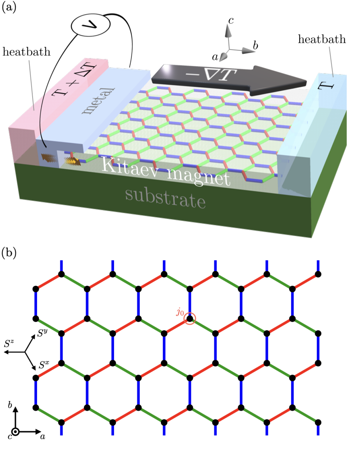
Figure 1: (a) Schematic of an experimental setup for measuring the spin Seebeck effect in Kitaev magnets. A Kitaev magnet placed on a substrate is attached to heatbaths from two sides to generate a temperature gradient. A metal with strong spin-orbit coupling, e.g., Pt, is sandwiched at one end. Due to the inverse spin Hall effect, the spin current is converted into a voltage perpendicular to the thermal gradient in the metal, which is observable. (b) Kitaev model on a honeycomb lattice used in simulations. The black dots represent the spin-1/2 degrees of freedom, and the red, blue, and green lines represent the $x$, $y$, and $z$ bonds, respectively [see Eq. (1)]. The lattice with $X=4$ and $L=12$ is shown, where $X$ is the number of spins in the vertical direction and $L$ is those in the horizontal direction. We impose an open boundary condition in the horizontal direction and a periodic boundary condition in the vertical direction. The $a$, $b$, and $c$ axes and $S^{x}$, $S^{y}$, and $S^{z}$ axes are shown in the inset. $j_{0}$ denotes the site where the local dynamical spin susceptibility is calculated.

The spin Seebeck effect refers to a phenomenon in which a spin current is induced by a thermal gradient. This effect is widely used as a sensitive probe for elementary excitations in magnets [50, 51, 52, 53, 54, 55, 56, 57]. In fact, in ordinary ferromagnets and antiferromagnets, the spin Seebeck effect is induced by magnon excitations from the conventional magnetic ordered state. Recently, this probe has been extended to more nontrivial magnets, such as those with frustrated interactions and low dimensionality, whose elementary excitations may have both positive and negative spin angular momenta, or even become spinless. The representative example is a negative spin Seebeck effect observed in a quantum spin liquid in a quasi-one-dimensional antiferromagnet [58]. This peculiar behavior, in contrast to conventional ferromagnets, was ascribed to fractional spinon excitations forming the Tomonaga–Luttinger liquid. Besides, other systems with strong quantum fluctuations, such as a spin-nematic liquid [59], a spin-Peierls system [60], and a magnon Bose–Einstein condensation system [61], have also been reported to exhibit the peculiar spin Seebeck effect. To the best of our knowledge, however, no study of quantum spin liquids in more than one dimension has been reported thus far. Recently, unconventional spin transport mediated by Majorana excitations in the KSL was reported [62, 63, 64, 65]. Meanwhile, as mentioned above, Majorana excitations were detected by thermal Hall measurements [33, 34, 35, 36, 37]. However, it remains unclear how the spin Seebeck effect, which involve both spin and heat transport, is manifested in the KSL and whether it is useful to identify, generate, and control the fractional excitations.

In this paper, we theoretically analyze the spin current induced by a thermal gradient via the spin Seebeck effect in the KSL. The possible experimental setup is shown in Fig. 1(a); we consider a bilayer junction of a Kitaev magnet and a paramagnetic metal, and calculate the tunnel spin current through the interface by the local dynamical spin susceptibility in an applied magnetic field, based on the tunnel spin-current theory [66, 67]. Accurately calculating the dynamics of quantum many-body problems, particularly in more than one spatial dimension, poses a significant challenge. In addressing this issue, we opt for a state-of-the-art numerical technique, real-time dynamics simulations based on the time-dependent variational principle (TDVP) [68] with matrix product states (MPSs) [69, 70]. We also complementarily conduct the analysis based on the perturbation theory with respect to the magnetic field for the KSL, as well as the linear spin-wave theory for the field-induced ferromagnetic (FFM) state. As a result, we find that the spin current is induced by a thermal gradient in the KSL mediated by the low-energy fractional Majorana quasiparticles that have no spin angular momentum. This is qualitatively different from the fact that fractional spinons in forming a one-dimensional Tomonaga–Luttinger liquid induce a negative spin Seebeck effect since the spinon has spin-$1/2$. It is remarkable that the quasiparticles without angular momentum can contribute to the tunnel spin-current transport. Furthermore, we find that the sign of the tunnel spin current depends on the sign of the Kitaev interaction; namely, the ferromagnetic (FM) and AFM KSLs lead to a positive and negative spin Seebeck effect, respectively. This is in stark contrast to the behavior in conventional ferromagnetic states where the magnon excitations lead to a positive spin Seebeck effect. In addition, we find that the KSLs show distinctive field angle dependence of the spin current that is different from those of the FFM states. These peculiar behaviors, which are ascribed to the spin current mediated by fractional Majorana excitations, are revealed for the first time to our knowledge by using the state-of-the-art numerical technique. In turn, our findings suggest the possibility of generating and controlling the Majorana excitations by spin injection.

The structure of this paper is as follows. In Sec. II, we describe the model and method used in this study. After introducing the Kitaev model under an external magnetic field, we describe the tunnel spin-current theory and numerical methods of real-time dynamics simulations to compute the spin Seebeck effect. We also mention the choice of model parameters and the details of calculation conditions. In Sec. III, we present the results of the real-time dynamics simulations, the perturbation analysis, and the linear spin-wave theory. In Sec. IV, we discuss the contrasting behaviors of the tunnel spin current depending on the sign of the Kitaev interaction, and the strength and direction of the magnetic field, which are important for experimental confirmation. Finally, Sec. V is devoted to summary.

II Model and method

We consider the Kitaev model [24] under an external magnetic field on a honeycomb lattice. The Hamiltonian reads

$$\mathcal{H}=K\sum_{\gamma}\sum_{\langle j,j^{\prime}\rangle_{\gamma}}S^{\gamma}_{j}S^{\gamma}_{j^{\prime}}-\sum_{j}{\bf B}\cdot{\bf S}_{j},$$ (1)

where the first term represents the bond-dependent Ising-type Kitaev interaction with the coupling constant $K$ and the second term denotes the Zeeman coupling with the magnetic field ${\bf B}$. The sums of $\gamma$ and $\langle j,j^{\prime}\rangle_{\gamma}$ run over $\{x,y,z\}$ and all the $\gamma$ bonds, respectively [see Fig. 1(b)]; ${\bf S}_{j}=(S^{x}_{j},S^{y}_{j},S^{z}_{j})$ represents the spin-$1/2$ operators at $j$ site. The $g$ factor and the Bohr magneton $\mu_{\rm B}$ are omitted in the Zeeman coupling term. We take $K=-1$ and $+1$ for the FM and AFM couplings, respectively.

We investigate the spin Seebeck effect in the Kitaev model in Eq. (1) based on the tunnel spin-current theory [66, 67, 60, 71]. The experimental setup is shown in Fig. 1(a); the spin Seebeck effect is measured by the inverse spin Hall effect [72, 73, 74] in a metal with strong spin-orbit coupling, such as Pt, attached to a Kitaev magnet. In the tunnel spin-current theory, spin injection is assumed to occur locally through the interface between the metal and the magnet, and calculated under the following conditions: (i) The interaction between the metal and the magnet is small enough to be dealt with as a perturbation and conserves angular momenta, (ii) the polarization of the tunnel spin current is parallel to the direction of the magnetic field, (iii) the temperature difference between the metal and the magnet is small, and (iv) the metal is nonmagnetic with featureless density of states in the low-energy region. It is worth noting that although the total magnetization is not conserved in the Kitaev model, these assumptions allow us to evaluate the tunnel spin current transferred to the metal that is detected in experiments.

On these assumptions, the tunnel spin current induced by a thermal gradient is evaluated by the perturbation theory with respect to the interface interaction using the nonequilibrium Green function method [75, 76, 77]. The expression is given by

$$\tilde{J}_{S}= \int_{-\infty}^{\infty}d\omega\,k\left(\frac{\omega}{T}\right)\,{\rm Im}\chi^{-+}_{\rm loc}(\omega),$$ (2)

up to a constant coefficient proportional to the temperature difference between the metal and magnet. The local dynamical spin susceptibility of the magnet, $\chi^{-+}_{\rm loc}(\omega)$, is defined as

$$\chi^{-+}_{\rm loc}(\omega)\equiv-i\int_{0}^{\infty}dt\langle\big{[}S^{-}_{j_{0}}(t),S^{+}_{j_{0}}(0)\big{]}\rangle e^{i\omega t-\delta t},$$ (3)

with the dumping factor $\delta$; $S^{\pm}_{j_{0}}$ is defined according to the direction of the magnetic field, namely,

$$S^{\pm}_{j_{0}}=S_{j_{0}}^{\tilde{x}}\pm iS_{j_{0}}^{\tilde{y}},$$ (4)

where $\tilde{x}$ and $\tilde{y}$ represent the directions perpendicular to the magnetic field along $\tilde{z}$ (the $\tilde{x}\tilde{y}\tilde{z}$ coordinate form a right-handed system) . In Eq. (2), the integral kernel $k(x=\omega/T)$ is given by

$$k(x)=\frac{x^{2}}{\sinh^{2}\big{(}x/2\big{)}},$$ (5)

with the temperature $T$ and the angular frequency $\omega$ (the Boltzmann constant and the Dirac constant are set to be unity). This factor $k(\omega/T)$ stems from the dynamical susceptibility of the metal and the temperature difference at the interface [67, 71]. Since $k(\omega/T)$ is an even function of $\omega$, Eq. (2) is written as

$$\tilde{J}_{S}= \int_{-\infty}^{\infty}d\omega\,k\left(\frac{\omega}{T}\right)\,[X_{+}(\omega)+X_{-}(\omega)]$$

$$= \int_{-\infty}^{\infty}d\omega\,k\left(\frac{\omega}{T}\right)\,X_{+}(\omega),$$ (6)

where $X_{\pm}(\omega)$ are the symmetric and antisymmetric components of ${\rm Im}\chi^{-+}_{\rm loc}(\omega)$, defined as

$$X_{\pm}(\omega)=\frac{1}{2}{\rm Im}\big{[}\chi^{-+}_{\rm loc}(\omega)\pm\chi^{-+}_{\rm loc}(-\omega)\big{]}.$$ (7)

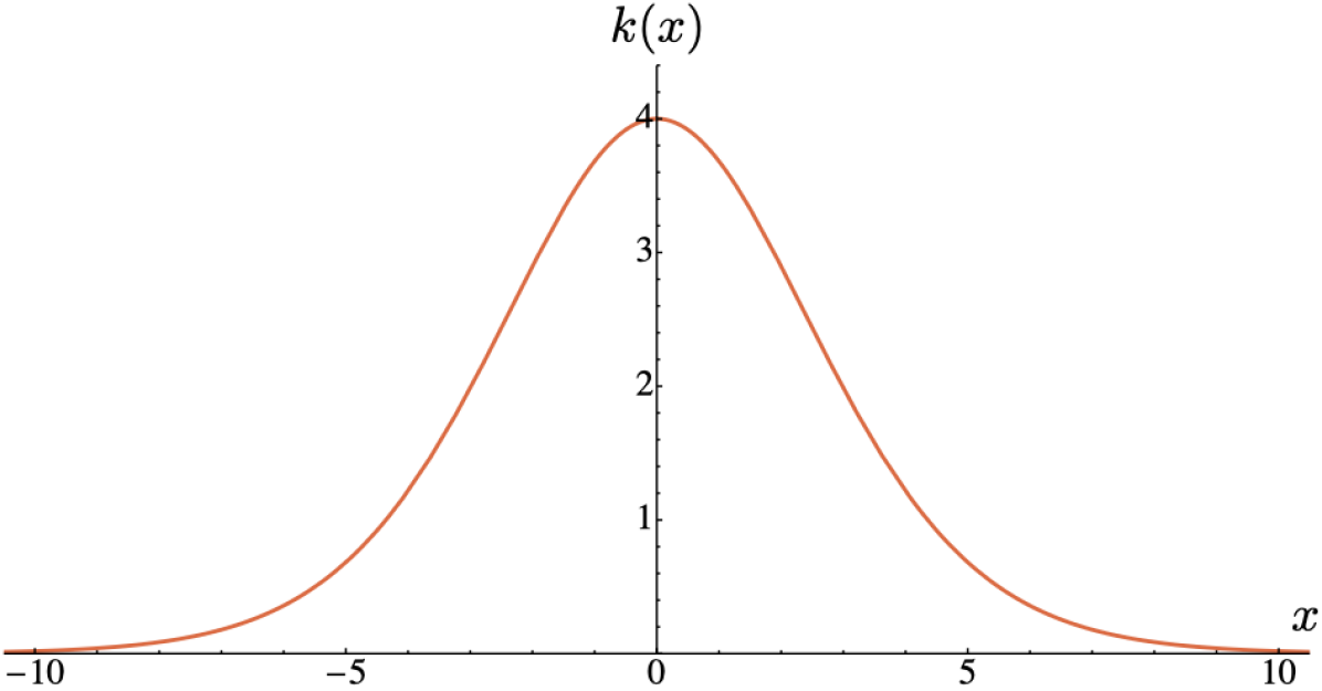
Figure 2: $x(=\omega/T)$ dependence of the integral kernel $k(x)$.

Equation (6) shows that only the symmetric component of ${\rm Im}\chi^{-+}_{\rm loc}(\omega)$ contributes to the tunnel spin current. The kernel $k(\omega/T)$ has a peak at $\omega=0$ and decays quickly for large $|\omega|/T$; hence, it works as a low-pass frequency filter at each $T$. Figure 2 shows the $\omega/T$ dependence of $k(\omega/T)$. The relevant frequency range is $|\omega/T|\lesssim 5$, and it becomes wider for higher temperature; for instance, at $T=0.01$, $X_{+}(\omega)$ for $|\omega|\lesssim 0.05$ is relevant to the tunnel spin current, and at $T=0.04$, $X_{+}(\omega)$ for $|\omega|\lesssim 0.2$ is relevant. We note that the tunnel spin current is always positive in the high-temperature limit, since the kernel becomes constant as $\lim_{T\to\infty}k(\omega/T)=4$ and the sum rule $\int_{0}^{\infty}X_{+}(\omega)d\omega=2\pi M$ holds ($M$ is the average of spin moment in the field direction): $\lim_{T\to\infty}\tilde{J}_{S}=8\pi M$.

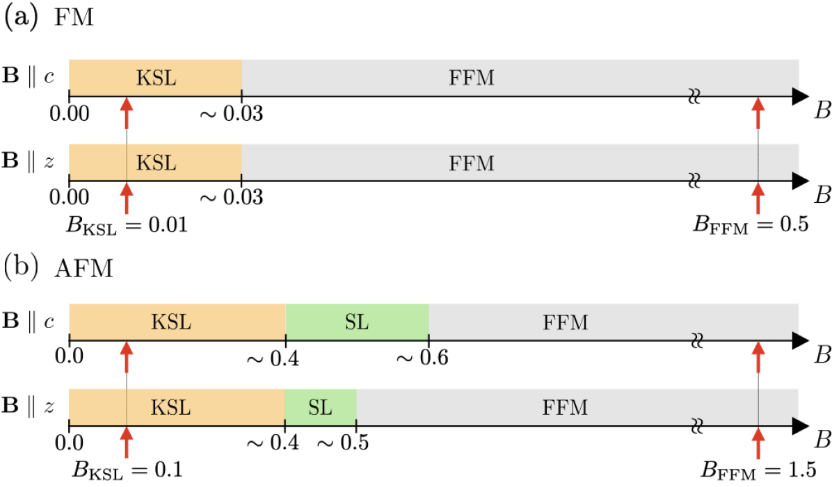
Figure 3: Schematic ground-state phase diagrams for the Kitaev model under the magnetic field $B$ for the (a) FM and (b) AFM cases. The magnetic field directions are ${\bf B}\parallel c$ in the upper panel and ${\bf B}\parallel z$ in the lower panel in each figure. The magnetic fields used in the present calculations, $B_{\rm KSL}$ and $B_{\rm FFM}$ are indicated by the red arrows. The values of the critical fields are taken from Refs. [79, 80, 81, 82].

In this study, we compute the tunnel spin current in an applied magnetic field ${\bf B}$ along the $\tilde{z}(=z$, $a$, $b$, or $c)$ axis [see Fig. 1(b)], and mainly discuss the cases of ${\bf B}\parallel z$ and ${\bf B}\parallel c$; the former gives the Zeeman coupling as $-BS_{j}^{z}$, while the latter gives $-B(S_{j}^{x}+S_{j}^{y}+S_{j}^{z})/\sqrt{3}$ in the second term in Eq. (1). In the calculations of $X_{+}(\omega)$, we choose $S_{j_{0}}^{\pm}$ as $S_{j_{0}}^{\pm}=S_{j_{0}}^{x}\pm iS_{j_{0}}^{y}$ for ${\bf B}\parallel z$, and $S_{j_{0}}^{\pm}=S_{j_{0}}^{a}\pm iS_{j_{0}}^{b}$ for ${\bf B}\parallel c$ (cyclic permutations for ${\bf B}\parallel a$ and ${\bf B}\parallel b$). We investigate the low-field KSL as well as the high-field FFM state for comparison. The phase transition from the KSL to the FFM state was studied by using the exact diagonalization, the density matrix renormalization group (DMRG) [83, 84], and Majorana mean-field approximation [79, 80, 81, 82]. The phase diagram is different between the FM and AFM cases not only quantitatively but also qualitatively, as shown in Fig. 3. In the FM case, the KSL turns into the FFM state at $B\approx 0.03$ for both ${\bf B}\parallel c$ [79, 80, 82] and ${\bf B}\parallel z$ [81]; there is a single phase transition. Meanwhile, in the AFM case, the values of the critical field become one order of magnitude larger, and moreover, the system exhibits another phase transition in addition to that to the FFM state. For ${\bf B}\parallel c$, the KSL is stable up to $B\approx 0.4$, and a different spin liquid (SL) takes place before entering into the FFM state at $B\approx 0.6$ [80, 82]. For ${\bf B}\parallel z$, the KSL is stable up to $B\approx 0.4$, and the intermediate SL is predicted to be stable up to $B\approx 0.5$ [81]. With reference to these studies, we choose the values of $B$ for the KSL (FMM) state, $B_{\rm KSL}$ ($B_{\rm FFM}$), well below (above) the critical fields: $B_{\rm KSL}=0.01$ and $B_{\rm FFM}=0.5$ for the FM case, and $B_{\rm KSL}=0.1$ and $B_{\rm FFM}=1.5$ for the AFM case, as indicated by the red arrows in Fig. 3.

In the following calculations, we compute $\chi^{-+}_{\rm loc}(\omega)$ in Eq. (3) at zero temperature for simplicity. This leaves the temperature dependence of the tunnel spin current only in the kernel $k(\omega/T)$. This assumption should be justified at sufficiently low temperature, especially below the crossover temperature $T\approx 0.016$ where the $Z_{2}$ flux excitations are almost absent [85]. To compute $\chi^{-+}_{\rm loc}(\omega)$ at $T=0$, we perform a real-time dynamics simulations based on TDVP [86]. The initial states of the simulations are obtained by multiplying $S^{\pm}_{j_{0}}$ to the MPS ground states computed by DMRG with the bond dimension $400$. We consider a cylinder-shaped lattice structure with the periodic (open) boundary condition in the vertical (horizontal) direction, as shown in Fig. 1(b), of the system size $X\times L$ with $(X,L)=(4,12)$, $(4,16)$, $(6,6)$, $(6,8)$, and $(6,10)$, where $X$ and $L$ are the number of sites in the vertical and horizontal directions, respectively, and employ the MPS representation wrapping around the cylinder in a snake form. We note that the ground state is not degenerate for all cases at the chosen magnetic fields. In Eq. (3), we choose $j_{0}$ at the site close to the center of each cylinder, as shown in Fig. 1(b), and take $\delta=0.01$. We set one time step of real-time dynamics as $\Delta t=0.2$ and perform $N_{t}=10^{4}$ time evolutions: Simulations are performed up to a maximum time $t_{\rm max}=2000$. When performing the Fourier transform [Eq. (3)], we interpolate the data by a cubic spline. The calculations are performed using a software library iTensor [87]. In addition, to understand the simulation results, we analyze the dynamical spin susceptibility based on the perturbation theory with respect to the magnetic field and the linear spin-wave theory, as described in Secs. III.2 and III.3, respectively.

III Results

III.1 Real-time dynamics simulations

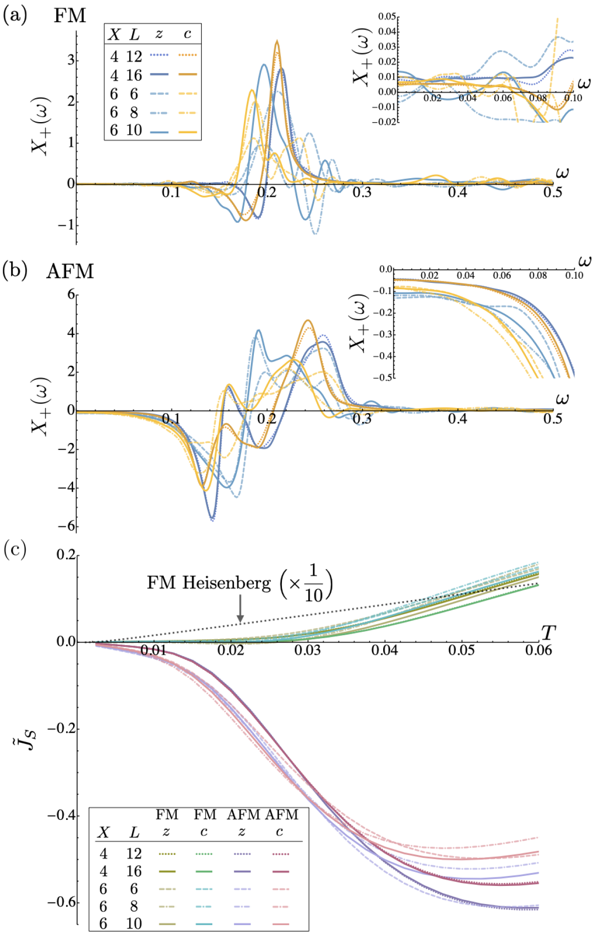
Figure 4: Results of real-time dynamics simulations in the KSL at $B=B_{\rm KSL}$. (a) and (b) show the $\omega$ dependences of $X_{+}(\omega)$ [Eq. (7)] for the FM and AFM Kitaev models, respectively. The insets are the enlarged plots in the low-frequency region. The different line colors and types represent the different field directions and the system sizes, respectively. (c) shows the temperature dependences of the tunnel spin current $\tilde{J}_{S}$ [Eq. (6)]. The black dotted line in (c) is a reference data for the $S=1/2$ FM Heisenberg model at $B=0.01$, multiplied by a factor of $1/10$ for better visibility (see Appendix A).

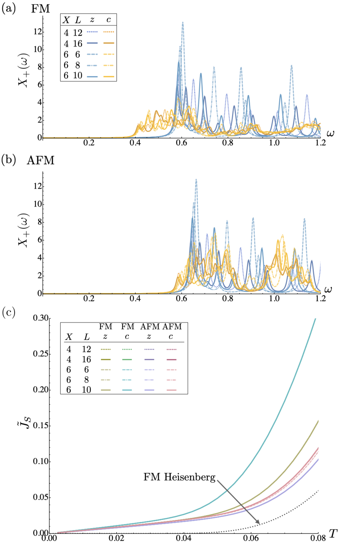
Figure 5: Results in the FFM state at $B=B_{\rm FFM}$. The notations are common to those in Fig. 4. The black dotted line in (c) is a reference data for the $S=1/2$ FM Heisenberg model at $B=0.5$ (see Appendix A).

We present the results of the real-time dynamics in the KSL at a low magnetic field $B=B_{\rm KSL}$ (see Fig. 3) obtained by TDVP in Fig. 4. Figures 4(a) and 4(b) show the symmetrized dynamical spin susceptibility $X_{+}(\omega)$ [Eq. (7)] for the FM and AFM Kitaev models, respectively, and Fig. 4(c) summarizes the tunnel spin current $\tilde{J}_{S}$ [Eq. (6)]. First of all, we show that, in both FM and AFM KSL states, the tunnel spin current is induced at finite temperature. In addition, we find a clear difference in the temperature dependence between the FM and AFM cases: $\tilde{J}_{S}$ is suppressed at low $T$, experiencing growth with a positive value as $T$ increases for the FM case, but it takes on a largely negative value in the AFM case. This trend is consistently observed across different system sizes and geometries. The origin can be traced back to the $\omega$ dependence of $X_{+}(\omega)$. In the FM case, $X_{+}(\omega)$ is small in the low-$\omega$ regime; the data are overall positive, but still scattered due to the finite-size effects, as shown in Fig. 4(a). In the larger-$\omega$ region, $X_{+}(\omega)$ exhibits a large positive intensity after a small negative dip, leading to the positive growth of $\tilde{J}_{S}$ with increasing $T$ in Fig. 4(c). In contrast, in the AFM case, $X_{+}(\omega)$ is developed with a negative value from the low- to intermediate-$\omega$ regime irrespective of the system sizes as shown in Fig. 4(b), which contributes to the largely negative $\tilde{J}_{S}$ in Fig. 4(c). Notably, while the finite-size effects are noticeable in $X_{+}(\omega)$ for the clusters accessible by the state-of-the-art numerical technique, those pertaining to $\tilde{J}_{S}$ are relatively small, showing the definite trend in the temperature dependence. We therefore conclude that, in the KSL state under the magnetic field, the tunnel spin current is thermally induced with opposite signs depending on the sign of the Kitaev interaction $K$.

This is in stark contrast to the behaviors in the FFM state at a high field $B=B_{\rm FFM}$. The results are shown in Fig. 5. In this case, $X_{+}(\omega)$ is overall positive, including the low-$\omega$ region, for both FM and AFM cases, as shown in Figs. 5(a) and 5(b). This leads to the tunnel spin current with positive sign for both cases, as shown in Fig. 5(c). These behaviors are confirmed by the linear spin-wave theory in Sec. III.3.

The contrasting behaviors between the KSL and FFM states can be ascribed to the fact that the carriers of the spin current are different between the two states. In the high-field FFM state, the elementary excitations are conventional magnons, which give a positive spin current irrespective of the details of the magnetic coupling. In contrast, in the low-field KSL state, the spin degree of freedom is fractionalized into itinerant Majorana fermions and localized $Z_{2}$ fluxes. They are independent of each other under magnetic fields, but in a low-field and low-temperature regime, the spin current in the KSL is expected to be carried predominantly by the itinerant Majorana fermions. The remarkable sign difference of $\tilde{J}_{S}$ between the FM and AFM Kitaev models suggests that the nature of Majorana fermions is different between the FM and AFM KSLs. This is a qualitatively different result from the one-dimensional antiferromagnet, where the spinon-mediated spin current was found to be negative [59]. We will discuss this sign switching by using the Majorana representation and the perturbation theory with respect to the magnetic field in Sec. III.2.

Let us make two remarks. The first one is on the magnitude of the tunnel spin current, $|\tilde{J}_{S}|$. In the KSL, $|\tilde{J}_{S}|$ increases much faster with temperature in the case of AFM than FM. Since the field strength $B$ is different and the low-field phase diagrams look different between the two cases, it is difficult to conclude that this is a general tendency. Nevertheless, $|\tilde{J}_{S}|$ are sufficiently large to be observed in experiments in both FM and AFM cases. This is explicitly shown by the comparison with the prototypical FM Heisenberg model, whose tunnel spin current is plotted by the black dotted line in Fig. 4(c) (see Appendix A for the details). Note that the spinon-mediated spin current was observed in the previous experiment [58], even though it is supposed to be smaller than the magnon-mediated one by a factor of $10^{-3}$–$10^{-4}$. Meanwhile, in the FFM state, $|\tilde{J}_{S}|$ is almost the same at low temperature regime in FM and AFM. This is due to almost the same magnitude of Zeeman gap in FM and AFM, as shown in Figs. 5(a) and 5(b), which is further confirmed by the linear spin-wave theory in Sec. III.3. Figure 5(c) also shows $\tilde{J}_{S}$ for the FM Heisenberg model at $B=0.5$ for comparison; the magnitude is much smaller than the result for $B=0.01$ shown in Fig. 4(c) because of the larger Zeeman gap, but it is comparable to those for the FFM states in the FM and AFM Kitaev models.

The second remark is on the dependence on the field direction. In Fig. 4(c), the tunnel spin currents in the low-field KSL show almost the same temperature dependences for ${\bf B}\parallel z$ and ${\bf B}\parallel c$. We confirm that the results for ${\bf B}\parallel a$ and ${\bf B}\parallel b$ are also similar (not shown). We will discuss this point in comparison with the results by the perturbation theory in Secs. III.2 and IV.2. Meanwhile, in the high-field FFM state, we find that ${\bf B}\parallel z$ gives rise to smaller tunnel spin currents than ${\bf B}\parallel c$ in both FM and AFM cases as shown in Fig. 5(c), reflecting the larger Zeeman gap observed in the spectra of $X_{+}(\omega)$ in Figs. 5(a) and 5(b) . We will also discuss this issue in comparison with the results by the linear spin-wave theory in Secs. III.3 and IV.2.

III.2 Perturbation analysis

To examine the origin of the different sign of $\tilde{J}_{S}$ between the FM and AFM KSLs in Fig. 4(c), we calculate the tunnel spin current in terms of Majorana fermions by using the perturbation theory with respect to the magnetic field. By using a Majorana fermion representation based on the Jordan-Wigner transformation [89, 90, 91], the Kitaev Hamiltonian at zero field in the flux free sector (the eigenstates without $Z_{2}$ flux excitations) is represented as

$$\mathcal{H}_{0}=-i\frac{K}{4}\sum_{\gamma}\sum_{\langle j,j^{\prime}\rangle}c_{j}c_{j^{\prime}}$$ (8)

with the Majorana fermion operators $c_{j}$. Based on the general framework of the perturbation theory [92], we obtain the effective operator of $S^{+}_{j_{0}}$ in the flux free sector through a transformation by $\Gamma:=PP_{0}(P_{0}PP_{0})^{-1/2}$, where $P_{0}$ and $P$ are projectors to the flux free sector of the unperturbed Hamiltonian [Eq. (1) for $B=0$] and to the states of the full Hamiltonian that are adiabatically connected to those in the flux free sector at $B=0$, respectively. By expanding up to the second order with respect to $B=|{\bf B}|$, the effective operator is obtained as

$$\Gamma^{\dagger}S^{+}_{j_{0}}\Gamma\sim s^{+(1)}+s^{+(2)}_{1}+s^{+(2)}_{2}=:s^{+}_{j_{0}},$$ (9)

where $s^{+(1)}$ and $s^{+(2)}_{1,2}$ are the first and second order contributions with respect to $B$, respectively; $s^{+(1)}$ and $s^{+(2)}_{1}$ are quadratic with respect to the Majorana fermion operators, while $s^{+(2)}_{2}$ is quartic, as

$$s^{+(1)}\simeq \frac{2}{|K|}\sum_{\gamma}B^{\gamma}A^{\gamma}\Big{[}S_{j_{0}}^{\gamma}S_{j_{\gamma}}^{\gamma}+\big{(}S^{\gamma}_{j_{0}}\big{)}^{2}\Big{]}$$

$$= \frac{1}{2|K|}\sum_{\gamma}B^{\gamma}A^{\gamma}\big{(}1-ic_{j_{0}}c_{j_{\gamma}}\big{)},$$ (10)

$$s^{+(2)}_{1}\simeq \frac{6}{|K|^{2}}\Big{(}A^{x}B^{y}B^{z}S^{x}_{j_{0}}S^{y}_{j_{y}}S^{z}_{j_{z}}$$

$$+A^{y}B^{z}B^{x}S^{y}_{j_{0}}S^{z}_{j_{z}}S^{x}_{j_{x}}+A^{z}B^{x}B^{y}S^{z}_{j_{0}}S^{x}_{j_{x}}S^{y}_{j_{y}}\Big{)}$$

$$= -\frac{3i}{4|K|^{2}}\Big{(}A^{x}B^{y}B^{z}c_{j_{y}}c_{j_{z}}$$

$$+A^{y}B^{z}B^{x}c_{j_{z}}c_{j_{x}}+A^{z}B^{x}B^{y}c_{j_{x}}c_{j_{y}}\Big{)},$$ (11)

$$s^{+(2)}_{2}\simeq \frac{6}{|K|^{2}}\Big{(}A^{x}B^{y}B^{z}S^{x}_{j_{0}}S^{y}_{k_{y}}S^{z}_{l_{z}}$$

$$+A^{y}B^{z}B^{x}S^{y}_{j_{0}}S^{z}_{k_{z}}S^{x}_{l_{x}}+A^{z}B^{x}B^{y}S^{z}_{j_{0}}S^{x}_{k_{x}}S^{y}_{l_{y}}\Big{)}$$

$$= -\frac{3}{4|K|^{2}}\Big{(}A^{x}B^{y}B^{z}c_{j_{0}}c_{j_{x}}c_{k_{y}}c_{l_{z}}$$

$$+A^{y}B^{z}B^{x}c_{j_{0}}c_{j_{y}}c_{k_{z}}c_{l_{x}}+A^{z}B^{x}B^{y}c_{j_{0}}c_{j_{z}}c_{k_{x}}c_{l_{y}}\Big{)}.$$ (12)

Here, ${\bf B}=(B^{x},B^{y},B^{z})$ and $S^{+}_{j_{0}}=A^{x}S^{x}_{j_{0}}+A^{y}S^{y}_{j_{0}}+A^{z}S^{z}_{j_{0}}$. See Fig. 6 for the definition of lattice sites $j_{\gamma}$, $k_{\gamma}$, and $l_{\gamma}$. In the derivation, the energy of all the intermediate states measured from the ground state is set at $|K|$ for simplicity, as in Ref. [24]. The effective operator of $S^{-}_{j_{0}}$, $s^{-}_{j_{0}}=s^{-(1)}+s^{-(2)}_{1}+s^{-(2)}_{2}$, is given by replacing $A^{\gamma}$ by $(A^{\gamma})^{*}$. Then, the tunnel spin current is obtained by Eq. (3), where $S^{\pm}_{j_{0}}$ and $\mathcal{H}$ are replaced by $s^{\pm}_{j_{0}}$ and $\mathcal{H}_{0}$, respectively. When we use the spectral representation, $X_{+}(\omega)$ in Eq. (7) is written as

$$\left.X_{+}(\omega)\right|_{S^{\pm}_{j_{0}}\to s^{\pm}_{j_{0}},\mathcal{H}\to\mathcal{H}_{0}}=\delta\sum_{\ell}\frac{|\langle\ell|s^{-}_{j_{0}}|\emptyset\rangle|^{2}-|\langle\ell|s^{+}_{j_{0}}|\emptyset\rangle|^{2}}{(E_{\ell}-E_{\emptyset}-\omega)^{2}+\delta^{2}},$$ (13)

for $\omega>0$, where $|\emptyset\rangle$ is the ground state of the pure Kitaev model in the flux free sector [Eq. (8)], $E_{\emptyset}$ is the ground state energy, and $|\ell\rangle$ and $E_{\ell}$ represent an excited state and its energy, respectively. By straightforward calculations in terms of the Majorana operators, we find that the $\mathcal{O}(B^{2})$ contributions from $s^{+(1)}$ vanish in the numerator of Eq. (13), since all the states appear in pair satisfying $|\langle\ell|s^{-(1)}|\emptyset\rangle|=|\langle\ell^{\prime}|s^{+(1)}|\emptyset\rangle|$ with $E_{\ell}=E_{\ell^{\prime}}$ (see Appendix B). Note that there is no $\mathcal{O}(B)$ contribution either since $s^{\pm}$ does not contain $\mathcal{O}(B^{0})$ term for the flux-free state. Hence, the sum in Eq. (13) includes the $\mathcal{O}(B^{3})$ and $\mathcal{O}(B^{4})$ contributions. We therefore compute the lowest-order contribution of the tunnel spin current by

$$\tilde{J}_{S}\sim\frac{B^{3}}{|K|^{3}}\tilde{j}_{S},$$ (14)

with

$$\tilde{j}_{S} =\int_{-\infty}^{\infty}d\omega\,k\left(\frac{\omega}{T}\right)\,x_{+}(\omega),$$ (15)

$$x_{+}(\omega) =\lim_{B\to 0}\frac{|K|^{3}}{B^{3}}\left.X_{+}(\omega)\right|_{S^{\pm}_{j_{0}}\to s^{\pm}_{j_{0}},\mathcal{H}\to\mathcal{H}_{0}}.$$ (16)

We note that our perturbation analysis takes into account lower-order contributions than those in the third-order perturbation analysis in the seminal paper by A. Kitaev [24]. Although the latter is known to open a gap in the spectra of itinerant Majorana fermions depending on the field direction, the effect of such gap opening is not included in our analysis; it appears in the higher-order $\mathcal{O}(B^{5})$ contributions.

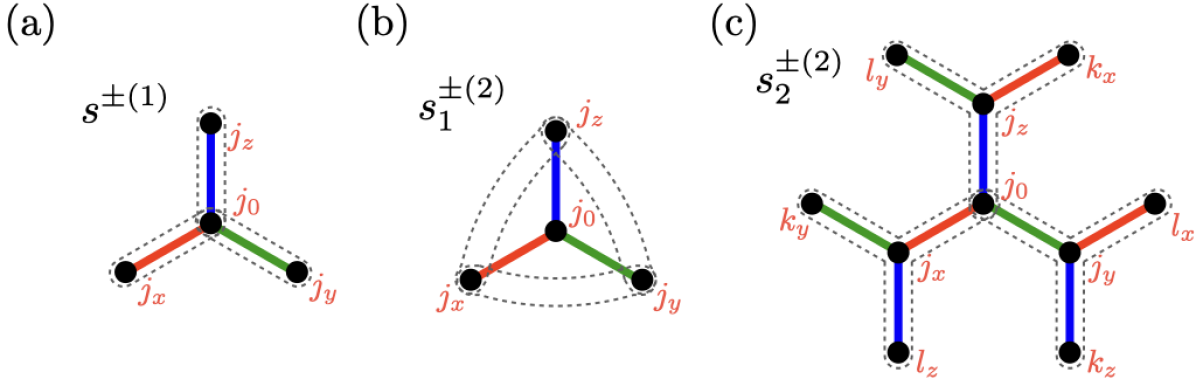
Figure 6: Pictorial descriptions of the effective operators (a) $s^{\pm(1)}$, (b) $s^{\pm(2)}_{1}$, and (c) $s^{\pm(2)}_{2}$. Each term is represented by the product of the Majorana operators at the two or four sites enclosed by the dashed lines.

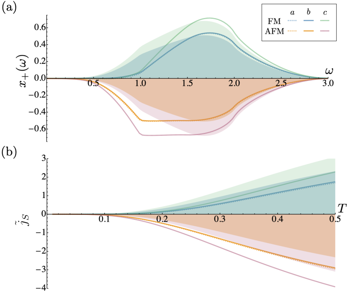
Figure 7: Results of the perturbation analysis for the FM and AFM Kitaev models in the weak magnetic field limit with ${\bf B}\parallel a$, ${\bf B}\parallel b$, and ${\bf B}\parallel c$: (a) $\omega$ dependences of $x_{+}(\omega)$ [Eq. (16)] and (b) temperature dependences of $\tilde{j}_{S}$ [Eq. (15)]. The lines represent the full results including all the contributions from $s^{+(1)}$ and $s_{1,2}^{+(2)}$, and the hatched regions represent the results ignoring $s^{\pm(2)}_{2}$. In the latter, ${\bf B}\parallel a$ and ${\bf B}\parallel b$ give the same results.

Figure 7 shows the results of the perturbation analysis. We find that $x_{+}(\omega)$ is mostly positive for the FM case (slightly negative at low $\omega$ for ${\bf B}\parallel a$ and ${\bf B}\parallel c$) and entirely negative for the AFM case, as shown in Fig. 7(a). This leads to positive and negative $\tilde{j}_{S}$ for the FM and AFM cases, respectively, as shown in Fig. 7(b). The result is in qualitative agreement with those of $\tilde{J}_{S}$ obtained by the TDVP simulations in Fig. 4(c).

The perturbation analysis provides a useful insight on the origin of the sign difference of the tunnel spin current between the FM and AFM cases. When we neglect the four Majorana contributions of $s_{2}^{\pm(2)}$, one can show that $x_{+}(\omega)$ in the FM and AFM cases are identical in the absolute value, but the signs are opposite. This is because the $\mathcal{O}(B^{3})$ contributions in Eq. (13) from the cross terms between $s^{\pm(1)}$ and $s^{\mp(2)}_{1}$ change their sign by $K\to-K$, i.e., $\langle\emptyset|s^{\mp(2)}_{1}|\ell\rangle\langle\ell|s^{\pm(1)}|\emptyset\rangle\to-\langle\emptyset|s^{\mp(2)}_{1}|\ell\rangle\langle\ell|s^{\pm(1)}|\emptyset\rangle$, due to the sign change in the eigenstates of Majorana fermions (see Appendix B). Consequently, the interchange of FM and AFM $K$ causes a sign reversal of $\tilde{j}_{S}$ in Eq. (15). The contributions with neglecting $s_{2}^{\pm(2)}$ are plotted by the hatched regions in Fig. 7. The result indicates that the contributions from the quadratic terms of the Majorana operators, $s^{\pm(1)}$ and $s^{\pm(2)}_{1}$, are dominant in $\tilde{j}_{S}$, and moreover, are the main cause of the sign switching of the tunnel spin current between the FM and AFM cases. The asymmetry between the two cases is due to the quartic terms in $s_{2}^{\pm(2)}$, leading to the faster growth of the tunnel spin current with temperature in AFM than FM, which is also consistent with the TDVP results in Fig. 4(c).

Let us make a remark on the $B$ dependence of the tunnel spin current. The perturbation theory in the low-field limit predicts $\tilde{j}_{S}\propto B^{3}$, but $\tilde{J}_{S}$ obtained by TDVP appears not to follow this asymptotic form; we find that $\tilde{J}_{S}$ at $B=B_{\rm KSL}/2$ is about half of that at $B=B_{\rm KSL}$ (not shown), suggesting that $\tilde{J}_{S}$ is roughly proportional to $B$. There are at least two possible reasons for this discrepancy. One is the contributions from excited states beyond the flux-free sector, which are neglected in the current perturbation analysis. The intermediate states [$|\ell\rangle$ in Eq. (13)] including flux excitations may give $\mathcal{O}(B)$ contributions, although they will be suppressed exponentially in the low-field limit because of the finite flux gap. If this is the case, the perturbation theory predict $\tilde{j}_{S}\simeq pB^{3}+qBe^{-\Delta_{\rm f}/T}$, where $\Delta_{\rm f}$ is the flux gap $\simeq 0.06|K|$ [24]. The other possibility is the limited system sizes in the TDVP simulations. Larger size simulations allow us to distinguish the $B$ dependence by accessing lower-field regions with higher precision by taking smaller dumping factor $\delta$ in Eq. (3). While such calculations require huge computational costs and are left for future study, this study comprehensively suggests that the coefficient $p$ and $q$ are both positive (negative) for the FM (AFM) KSL.

III.3 Linear spin-wave theory

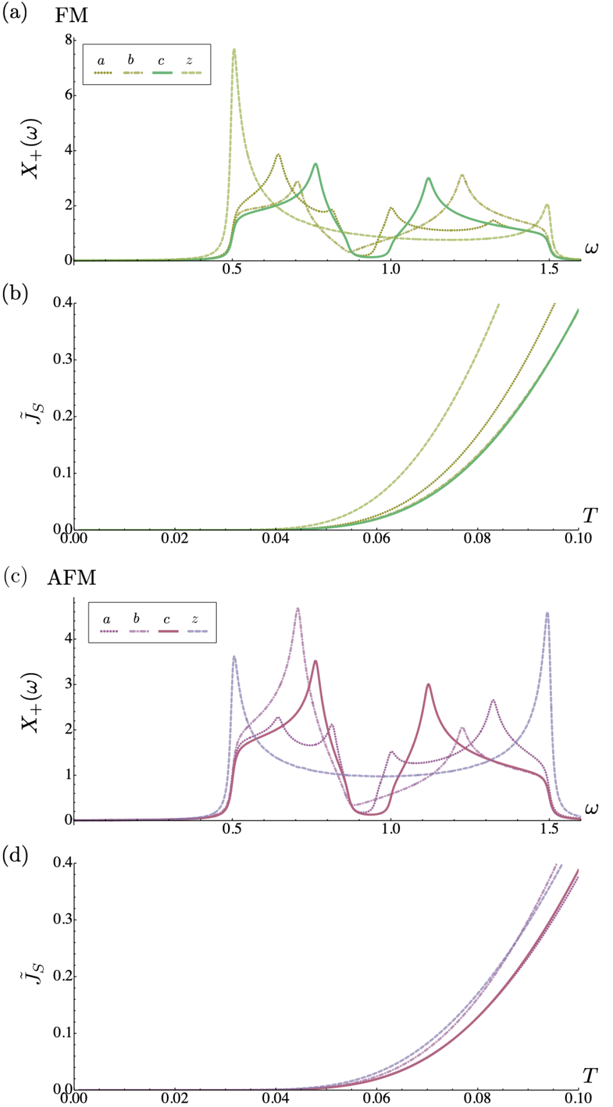
Figure 8: Results by the linear spin-wave theory for the (a,b) FM and (c,d) AFM Kitaev models at $B=B_{\rm FFM}$ with four field directions ${\bf B}\parallel a$, ${\bf B}\parallel b$, ${\bf B}\parallel c$, and ${\bf B}\parallel z$. (a) and (c) show the $\omega$ dependences of $X_{+}(\omega)$ for the FM and AFM cases, respectively. (b) and (d) show the temperature dependences of the tunnel spin current $\tilde{J}_{S}$.

In this section, we present the results obtained by the linear spin-wave theory for the Kitaev model in the FFM state, for comparison with the results in Fig. 5. The procedure to calculate the tunnel spin current is described for the FM Heisenberg model in Appendix A. We take the similar procedure by performing the diagonalization of the bosonic Hamiltonian and the calculations of $X_{+}(\omega)$ numerically.

Figure 8 shows the results for $B=B_{\rm FFM}$ (see Fig. 3) with four different field directions. We find that $X_{+}(\omega)$ is always positive for both FM and AFM cases, as shown in Figs. 8(a) and 8(c), respectively. These behaviors are in qualitative agreement with the TDVP simulation results shown in Figs. 5(a) and 5(b). The positive $X_{+}(\omega)$ leads to the tunnel spin current with positive sign as shown in Fig. 8(b). This is also in agreement with the TDVP simulation results in Fig. 5(c). We note, however, that the gap in the spectrum of $X_{+}(\omega)$ is independent of the field directions in the linear spin-wave theory, while it is considerably different between ${\bf B}\parallel z$ and ${\bf B}\parallel c$ in the TDVP simulation.

In Figs. 8(a) and 8(c), $X_{+}(\omega)$ shows a sharp peak at the lower edge of the spectrum for ${\bf B}\parallel z$ in both FM and AFM cases, while it shows a shoulder for the other field directions. These qualitative differences can be understood as follows. When ${\bf B}\parallel z$, the Holstein-Primakoff bosons cannot hop on the $z$ bonds and move only along one-dimensional zigzag chains composed of the $x$ and $y$ bonds, resulting in the logarithmic divergence in the spectrum. Meanwhile, for the other field directions, two-dimensional motion is allowed, which results in the shoulder-like feature in the spectrum. We note that these behaviors are not clearly seen in the TDVP simulation results [Figs. 5(a) and 5(b)], presumably due to finite-size effects and correlation between magnons.

IV Discussion

IV.1 Sign of spin current in Kitaev spin liquids

The real-time dynamics simulations based on TDVP reveal the sign switching of the tunnel spin current between the FM and AFM KSLs (Sec. III.1). This behavior is successfully reproduced by the perturbation theory in the Majorana representation (Sec. III.2). These findings indicate that the spin current in the KSL is predominantly carried by the itinerant Majorana fermions. More importantly, they suggest that the itinerant Majorana fermions contribute to the spin current with (up-)down-spin like nature in the (AFM) FM KSL where the sign of the tunnel spin current is (negative) positive, even though they do not have spin angular momentum.

The negative spin Seebeck effect that we find for the AFM KSL appears to be common to that for a quantum spin liquid in a quasi-one-dimensional antiferromagnet [58]. This implies common physics in the spin current carried by fractional excitations in AFM quantum spin liquids in one and two dimensions, even though the fractional quasiparticles have different nature: The spin angular momentum carried by a spinon in the one-dimensional quantum spin liquid is half quantized $\Delta S=1/2$, while that by a Majorana fermion in the KSL is not. Our results, however, indicate that the FM quantum spin liquid, which is peculiar to the Kitaev model, can induce a tunnel spin current with positive sign, suggesting that the spin Seebeck effect is useful to identify the nature of fractional quasiparticles in quantum spin liquids. We emphasize that our study reveals, for the first time to our knowledge, that the spin Seebeck effect in quantum spin liquids can be either positive or negative by analyzing both FM and AFM Kitaev models in two dimensions. Toward deeper understanding of the spin Seebeck effect in quantum spin liquids, further comparative studies are necessary for different types of quantum spin liquids in different dimensions. The simulation method for the real-time dynamics used in this study provides a powerful method to study generic models and awaits wider applications in the future.

Meanwhile, the spin Seebeck effect for the FM KSL has the same positive sign as that carried by conventional magnons in the FFM state. Thus, a way to distinguish between the two is needed. We will discuss this point in the next subsection.

IV.2 Magnetic field dependence of tunnel spin current

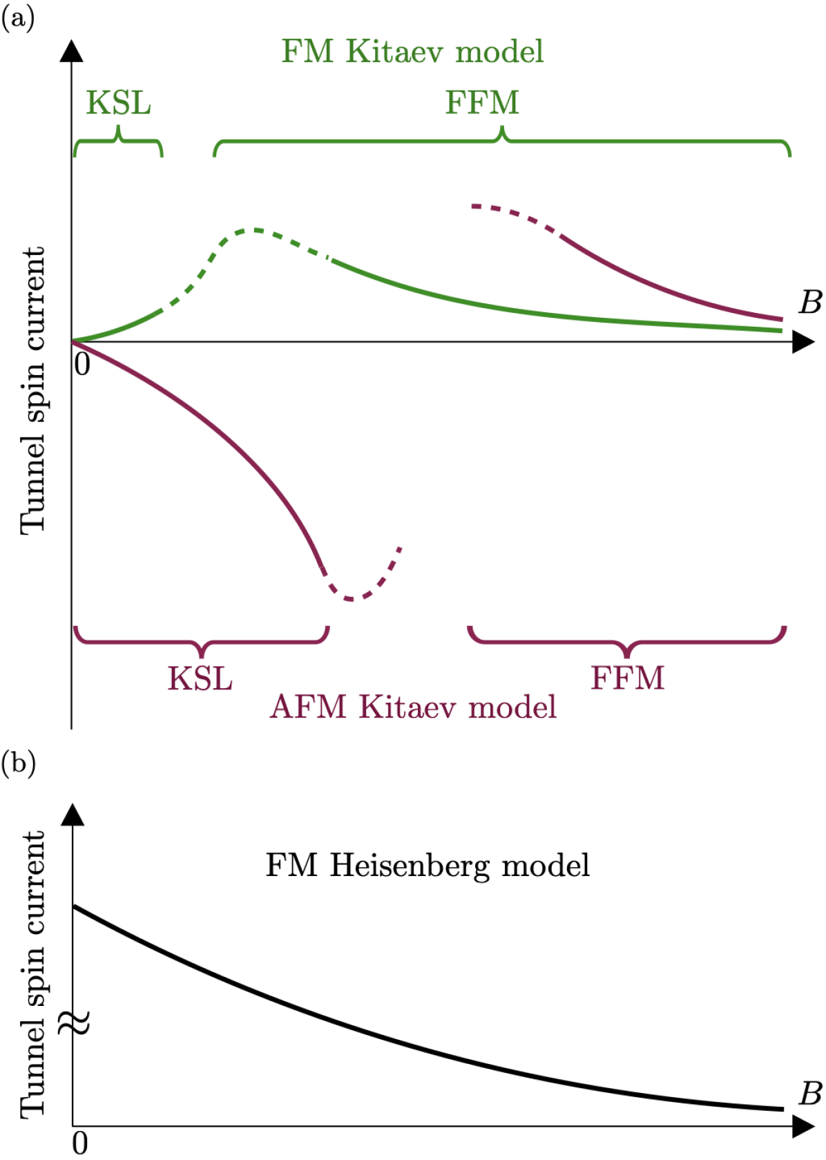
Figure 9: Schematics of the magnetic field dependence of the tunnel spin current caused by the spin Seebeck effect at low temperature for (a) the FM and AFM Kitaev models and (b) the FM Heisenberg model.

Based on the results by the real-time dynamics simulations, the perturbation theory, and the linear spin-wave theory, we show a schematic of the magnetic field dependence of the tunnel spin current caused by the spin Seebeck effect for the Kitaev model in Fig. 9(a). On one hand, in the low-field KSL region, the tunnel spin current increases in amplitude with increasing the field strength, with a different sign between the FM and AFM cases. As discussed in the end of Sec. III.2, a more detailed analysis is needed to fully elucidate the behavior in the low-field limit. On the other hand, in the high-field FFM regime, the tunnel spin current is positive for both FM and AFM cases and decreases with increasing the field strength as shown in Fig. 9(a). This is similar to the FM Heisenberg model [Fig. 9(b)]. Thus, these results imply that the tunnel spin current is maximized between the KSL and FFM states in the FM case, while it should change its sign in the AFM cases, as schematically shown in Fig. 9(a). However, further studies are needed to clarify the field dependence in those transient regions, including the another intermediate spin liquid region in the AFM case (see Fig. 3).

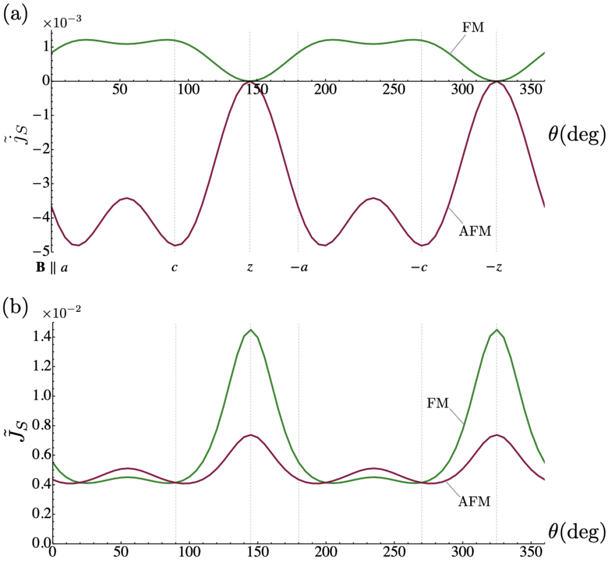
Figure 10: Field angle dependences of the tunnel spin current when the magnetic field is rotated in the $ac$ plane obtained by (a) the perturbation analysis for low $B$ and (b) the linear spin-wave theory at $B=B_{\rm FFM}$. The angle $\theta$ is measured from the $a$ axis, and the data are calculated at $T=0.05$. In (a), the lines represent the full results including all the contributions from $s^{+(1)}$ and $s_{1,2}^{+(2)}$, and the hatched regions represent the results ignoring $s^{\pm(2)}_{2}$.

Since the positive sign of the spin Seebeck effect is common between the FM KSL and the FFM state, a way to distinguish between the two is needed. One is the field dependence discussed above: $\tilde{J}_{S}$ increases with $B$ in the low-field KSL, but it decreases in the high-field FFM state. Another efficient way is the dependence on the magnetic field direction. Figure 10 shows the field angle dependence of the tunnel spin currents in the $ac$ plane (see Fig. 1): (a) The results for the low-field KSL obtained by the perturbation analysis and (b) those for the high-field FFM state by the linear spin-wave theory. In the perturbation theory, the tunnel spin current $\tilde{j}_{S}$ vanishes for ${\bf B}\parallel z$. This is because $s^{\pm(1)}$, $s^{\pm(2)}_{1}$, and $s^{\pm(2)}_{2}$ in Eqs. (10)–(12) are all zero for ${\bf B}\parallel z$, as $B^{x}=B^{y}=0$ and $A^{z}=0$. The same applies for ${\bf B}\parallel x$ and ${\bf B}\parallel y$. Thus, the tunnel spin current for the low-field KSL is minimized for ${\bf B}\parallel z$, while maximized for ${\bf B}\parallel c$. The other maxima with the same value as ${\bf B}\parallel c$ are found at $\theta\approx 20^{\circ}$ and $200^{\circ}$ due to the symmetry of $\pi$ rotation about the $[110]$ axis ($\theta\approx 54.7^{\circ}$). Meanwhile, the linear spin-wave theory for the FFM state predicts an opposite tendency: The tunnel spin current is maximized for ${\bf B}\parallel z$, while minimized for ${\bf B}\parallel c$, as shown in Fig. 10(b). This is due to the logarithmic divergence discussed in Sec. III.3. We note that the TDVP simulation data presented in Figs. 4 and 5, however, are not sufficient to discuss these issues presumably due to the limited system sizes. Further extensions are needed for more precise predictions for experiments.

V Summary

In summary, we have studied the spin Seebeck effect in both the ferromagnetic and antiferromagnetic Kitaev spin liquids by using the real-time dynamics simulation, the perturbation analysis, and the linear spin-wave theory, based on the tunnel spin-current theory. There are two main discoveries. The first one is that the spin Seebeck effect is induced in the Kitaev spin liquid by the low-energy fractional Majorana quasiparticles that have no spin angular momentum. This is a qualitatively different phenomenon from the spin Seebeck effect in the one-dimensional quantum spin liquid induced by the fractional spinon excitations with nonzero spin angular momentum. The second discovery is that the spin current mediated by elementary excitations in quantum spin liquids can be positive or negative; namely, we found the sign change of the spin current in the Kitaev spin liquid between the ferromagnetic and antiferromagnetic Kitaev interactions. Our finding suggests the Majorana fermions contribute to the spin current with up- and down-spin like nature in the ferromagnetic and antiferromagnetic Kitaev spin liquid, respectively. This finding refutes a possibility that the spin current carried by the fractional excitations is always negative in the quantum spin liquids.

Fractional excitations in quantum spin liquids are hard to identify by conventional experimental probes, since they behave very differently from the original spin degree of freedom and there is no conjugate field to directly excite them. Our finding suggests that the spin Seebeck effect make it possible and would be a powerful tool for investigating the nature of fractional excitations, in addition to the existing methods, such as the Raman scattering [93, 94, 95], the inelastic neutron scattering [96, 97, 98, 99, 100, 101, 102, 103], and the thermal Hall effect [33, 34, 35, 36, 37]. Furthermore, our results show that the Majorana quasiparticles in the Kitaev spin liquid can be driven by the spin current, suggesting the possibility of generating and controlling them by a spin injection. It is highly desired to confirm this phenomenon experimentally by using the setup in Fig. 1(a) for both ferromagnetic and antiferromagetic Kitaev magnets; the former includes several iridium oxides and $\alpha$-RuCl₃ [26, 27, 28], and the latter was theoretically predicted, e.g., for polar spin-orbit Mott insulators [104] and $f$-electron compounds [105, 106].

Appendix A Spin current in the ferromagnetic Heisenberg model

In this Appendix, we show how to compute the tunnel spin current $\tilde{J}_{S}$ in Eq. (6) for the FM Heisenberg model [67, 58, 71] shown in Fig. 4(c). The Hamiltonian reads

$$\mathcal{H}_{\rm H}=-J\sum_{\langle j,j^{\prime}\rangle}{\bf S}_{j}\cdot{\bf S}_{j^{\prime}}-\sum_{j}{\bf B}\cdot{\bf S}_{j},$$ (17)

where the sum of $\langle j,j^{\prime}\rangle$ is taken for all the nearest-neighbor spins on the honeycomb lattice; we take $J=1$. Without loss of generality, we consider ${\bf B}\parallel z$, for which all the spins are fully polarized to the $z$ direction in the ground state.

We calculate $\tilde{J}_{S}$ for the fully-polarized (FP) state by using the linear spin-wave theory. By the Holstein-Primakoff transformation, $S^{+}_{j}=b^{\;}_{j}$, $S^{-}_{j}=b^{\dagger}_{j}$, and $S^{z}_{j}=\frac{1}{2}-n_{j}$ with $n_{j}=b^{\dagger}_{j}b^{\;}_{j}$, the Hamiltonian is written by the boson operators $b^{\;}_{j}$ and $b^{\dagger}_{j}$ as

$$\mathcal{H}_{\rm H}= -\frac{J}{2}\sum_{\langle j,j\rangle}\left[(b^{\dagger}_{j}b_{j^{\prime}}+{\rm h.c.})-n_{j}-n_{j^{\prime}}\right]$$

$$-J\sum_{\langle j,j^{\prime}\rangle}n_{j}n_{j^{\prime}}+B\sum_{j}n_{j},$$ (18)

up to a constant, where $B=|{\bf B}|$. Ignoring the interaction term $n_{j}n_{j^{\prime}}$ and using the Fourier transformation, we obtain

$$\mathcal{H}^{\rm LSW}_{{\rm H}}= -\sum_{\bf r}\left(g_{\bf q}b^{\dagger}_{{\bf q}\rm B}b_{{\bf q}\rm A}+{\rm h.c.}\right)$$

$$+\big{(}\frac{3}{2}J+B\big{)}\sum_{{\bf q},\alpha}b^{\dagger}_{{\bf q}\alpha}b_{{\bf q}\alpha},$$ (19)

where $g_{\bf q}=(J/2)(e^{i{\bf q}\cdot{\bf a}_{1}}+e^{i{\bf q}\cdot{\bf a}_{2}}+1)$ with two translation vectors ${\bf a}_{1}$ and ${\bf a}_{2}$, and the index $\alpha$ denotes the sublattice A and B. This is easily diagonalized as

$$\mathcal{H}^{\rm LSW}_{{\rm H}}= \sum_{{\bf q}}\sum_{\sigma=\pm}\varepsilon_{{\bf q}\sigma}\eta^{\dagger}_{{\bf q}\sigma}\eta^{\;}_{{\bf q}\sigma},$$ (20)

where

$$\varepsilon_{{\bf q}\sigma}= \sigma|g_{\bf q}|+\frac{3}{2}J+B.$$ (21)

We note that the excitation spectra $\varepsilon_{{\bf q}\sigma}$ has a gap of $\Delta=B$ at ${\bf q}=0$.

For the FP state, the symmetrized dynamical spin susceptibility $X_{+}(\omega)$ [Eq. (7)] is represented by using the spectral representation as

$$X_{+}(\omega)= \frac{\delta}{2}\sum_{\ell}\frac{|\langle\ell|S^{-}_{j_{0}}|{\rm FP}\rangle|^{2}-|\langle\ell|S^{+}_{j_{0}}|{\rm FP}\rangle|^{2}}{(E_{\ell}-E_{\rm FP}-\omega)^{2}+\delta^{2}}$$

$$= \frac{\delta}{2}\sum_{\ell}\frac{|\langle\ell|S^{-}_{j_{0}}|{\rm FP}\rangle|^{2}}{(E_{\ell}-E_{\rm FP}-\omega)^{2}+\delta^{2}},$$ (22)

for $\omega>0$, where $|{\rm FP}\rangle$ and $E_{\rm FP}$ are the FP ground state and its energy, and $|\ell\rangle$ and $E_{\ell}$ are an excited state and its energy; the sum of $\ell$ runs over all the excited states. In the linear spin-wave theory, $X_{+}(\omega)$ is expressed in terms of boson operators as

$$X_{+}(\omega) =\frac{\delta}{2}\sum_{\ell}\frac{|\langle\ell|b^{\dagger}_{j_{0}}|{\rm FP}\rangle|^{2}}{(E_{\ell}-E_{\rm FP}-\omega)^{2}+\delta^{2}},$$ (23)

$$=\frac{\delta}{2N_{\rm u}}\sum_{{\bf q},\sigma}\frac{1}{(\varepsilon_{{\bf q}\sigma}-\omega)^{2}+\delta^{2}}$$ (24)

$$\xrightarrow[\delta\to 0]{}\ \frac{\pi}{2N_{\rm u}}\sum_{{\bf q},\sigma}\delta(\omega-\varepsilon_{{\bf q}\sigma}),$$ (25)

where $N_{\rm u}$ is the number of unit cells and we use the fact that $|{\rm FP}\rangle$ is a vacuum of bosons. Finally, using this expression, the tunnel spin current is obtained as

$$\tilde{J}_{S}= 2\int_{0}^{\infty}d\omega\,X_{+}(\omega)\,k\left(\frac{\omega}{T}\right)=\frac{\pi}{N_{\rm u}}\sum_{{\bf q},\sigma}k\left(\frac{\varepsilon_{{\bf q}\sigma}}{T}\right).$$ (26)

In the calculation of the data in Figs. 4(c) and 5(c), we take $N_{\rm u}=288^{2}$.

Appendix B Matrix elements of $s^{\pm(1)}$ and $s^{\pm(2)}_{1}$

In this Appendix, we show two relations for the matrix elements of $s^{\pm(1)}$ and $s^{\pm(2)}_{1}$ in Eq. (13) used in the perturbation analysis. Let us begin with diagonalization of the Majorana Hamiltonian for the flux free sector. By using the Fourier transformation

$$c_{{\bf r}\alpha}= \sqrt{\frac{2}{N_{\rm u}}}{\sum_{\bf q}}^{\prime}\left(\gamma_{{\bf q}\alpha}e^{+i{\bf q}\cdot{\bf r}}+\gamma^{\dagger}_{{\bf q}\alpha}e^{-i{\bf q}\cdot{\bf r}}\right),$$ (27)

where the sum runs over half of the first Brillouin zone with $q_{x}>0$ and $\alpha=A$ or B, Eq. (8) is rewritten as

$$\mathcal{H}_{0}= {\sum_{\bf q}}^{\prime}{\boldsymbol{\gamma}}^{\dagger}_{\bf q}\mathsf{H}_{\bf q}{\boldsymbol{\gamma}}^{\;}_{\bf q},$$ (28)

with

$$\mathsf{H}_{\bf q}= \left(\begin{matrix}0&if_{\bf q}\\ -if^{*}_{\bf q}&0\end{matrix}\right),$$ (29)

where ${\boldsymbol{\gamma}}^{\dagger}_{\bf q}=(\gamma^{\dagger}_{{\bf q}w}~{}\gamma^{\dagger}_{{\bf q}b})$ and $f_{\bf q}=(K/2)(e^{i{\bf q}\cdot{\bf a}_{1}}+e^{i{\bf q}\cdot{\bf a}_{2}}+1)$. The matrix $\mathsf{H}_{\bf q}$ is diagonalized by a unitary matrix,

$$\mathsf{U}_{\bf q}=\frac{1}{\sqrt{2}|f_{\bf q}|}\left(\begin{matrix}|f_{\bf q}|&if_{\bf q}\\ -if^{*}_{\bf q}&-|f_{\bf q}|\end{matrix}\right),$$ (30)

as $\mathsf{U}_{\bf q}^{\dagger}\mathsf{H}_{\bf q}\mathsf{U}_{\bf q}={\rm diag}(|f_{\bf q}|,-|f_{\bf q}|)$. Then, the Hamiltonian is diagonalized as

$$\mathcal{H}_{0}= {\sum_{\bf q}}^{\prime}\sum_{\sigma=\pm}\sigma|f_{\bf q}|\alpha^{\dagger}_{{\bf q}\sigma}\alpha^{\;}_{{\bf q}\sigma},$$ (31)

where ${\boldsymbol{\alpha}}^{\dagger}_{\bf q}=(\alpha^{\dagger}_{{\bf q}+}~{}\alpha^{\dagger}_{{\bf q}-})$, and ${\boldsymbol{\alpha}}^{\dagger}_{\bf q}={\boldsymbol{\gamma}}^{\dagger}_{\bf q}\mathsf{U}_{\bf q}$.

With these notations, the ground state $|\emptyset\rangle$ is expressed as

$$|\emptyset\rangle={\prod_{\bf q}}^{\prime}\alpha^{\dagger}_{{\bf q}-}|{\rm vac}\rangle,$$ (32)

where $|{\rm vac}\rangle$ is the vacuum for $\alpha$ fermions. Since the operators $s^{\pm(1)}$ and $s^{\pm(2)}_{1}$ [Eqs. (10) and (11)] have the quadratic forms of the Majorana fermion operators, we consider two-particle, two-hole, and particle-hole states as the intermediate states $|\ell\rangle$: $|{\bf q}+,{\bf q}^{\prime}+\rangle=\alpha^{\dagger}_{{\bf q}+}\alpha^{\dagger}_{{\bf q}^{\prime}+}|\emptyset\rangle$, $|{\bf q}-,{\bf q}^{\prime}-\rangle=\alpha_{{\bf q}-}\alpha_{{\bf q}^{\prime}-}|\emptyset\rangle$, and $|{\bf q}+,{\bf q}^{\prime}-\rangle=\alpha^{\dagger}_{{\bf q}+}\alpha_{{\bf q}^{\prime}-}|\emptyset\rangle$, respectively.

First, we show that all the intermediate states appear in pairs of $|\ell\rangle$ and $|\ell^{\prime}\rangle$, satisfying $|\langle\ell|s^{-(1)}|\emptyset\rangle|=|\langle\ell^{\prime}|s^{+(1)}|\emptyset\rangle|$ with $E_{\ell}=E_{\ell^{\prime}}$. Let us consider the two-particle and two-hole states, for which the matrix elements are given by

$$\langle{\bf q}-,{\bf q}^{\prime}-|s^{+(1)}|\emptyset\rangle=-\frac{1}{2N_{\rm u}|K|}\times$$

$$\left[\frac{f_{\bf q}}{|f_{\bf q}|}(B^{x}A^{x}e^{{i}{\bf q}^{\prime}\cdot{\bf a}_{1}}+B^{y}A^{y}e^{{i}{\bf q}^{\prime}\cdot{\bf a}_{2}}+B^{z}A^{z})-({\bf q}\leftrightarrow{\bf q}^{\prime})\right],$$ (33)

$$\langle{\bf q}^{\prime}+,{\bf q}+|s^{-(1)}|\emptyset\rangle=-\frac{1}{2N_{\rm u}|K|}\times$$

$$\biggl{[}\frac{f_{{\bf q}^{\prime}}}{|f_{{\bf q}^{\prime}}|}(B^{x}(A^{x})^{*}e^{-i{\bf q}^{\prime}\cdot{\bf a}_{1}}+B^{y}(A^{y})^{*}e^{-i{\bf q}^{\prime}\cdot{\bf a}_{2}}+B^{z}(A^{z})^{*})$$

$$\ \ -({\bf q}\leftrightarrow{\bf q}^{\prime})\biggr{]},$$ (34)

respectively, where $({\bf q}\leftrightarrow{\bf q}^{\prime})$ denotes the term with interchange of ${\bf q}$ and ${\bf q}^{\prime}$. From these two equations, we can show the relation

$$\langle{\bf q}-,{\bf q}^{\prime}-|s^{+(1)}|\emptyset\rangle^{*}=\langle{\bf q}^{\prime}+,{\bf q}+|s^{-(1)}|\emptyset\rangle\frac{f^{*}_{\bf q}f^{*}_{{\bf q}^{\prime}}}{|f^{*}_{\bf q}||f^{*}_{{\bf q}^{\prime}}|}.$$ (35)

Thus, we obtain

$$|\langle{\bf q}-,{\bf q}^{\prime}-|s^{+(1)}|\emptyset\rangle|=|\langle{\bf q}^{\prime}+,{\bf q}+|s^{-(1)}|\emptyset\rangle|.$$ (36)

Note that the energy of $|\ell\rangle=|{\bf q}-,{\bf q}^{\prime}-\rangle$ and $|\ell^{\prime}\rangle=|{\bf q}+,{\bf q}^{\prime}+\rangle$ are the same, since $E_{\ell}=E_{\ell^{\prime}}=|f_{\bf q}|+|f_{{\bf q}^{\prime}}|$. For the particle-hole states, the matrix element is given by

$$\langle{\bf q}+,{\bf q}^{\prime}-|s^{+(1)}|\emptyset\rangle=\frac{i}{2N_{\rm u}|K|}\times$$

$$\frac{1}{|f_{\bf q}||f_{{\bf q}^{\prime}}|}\biggl{[}(B^{x}A^{x}e^{+i{\bf q}^{\prime}\cdot{\bf a}_{1}}+B^{y}A^{y}e^{+i{\bf q}^{\prime}\cdot{\bf a}_{2}}+B^{z}A^{z})|f_{\bf q}||f_{{\bf q}^{\prime}}|$$

$$-(B^{x}A^{x}e^{-i{\bf q}\cdot{\bf a}_{1}}+B^{y}A^{y}e^{-i{\bf q}\cdot{\bf a}_{2}}+B^{z}A^{z})f_{{\bf q}}f_{{\bf q}^{\prime}}\biggr{]}.$$ (37)

Similarly to the two-particle and two-hole states, we can show

$$\langle{\bf q}+,{\bf q}^{\prime}-|s^{+(1)}|\emptyset\rangle^{*}=\langle{\bf q}^{\prime}+,{\bf q}-|s^{-(1)}|\emptyset\rangle\frac{f^{*}_{\bf q}f^{*}_{{\bf q}^{\prime}}}{|f^{*}_{\bf q}||f^{*}_{{\bf q}^{\prime}}|},$$ (38)

and thus, we obtain

$$|\langle{\bf q}+,{\bf q}^{\prime}-|s^{+(1)}|\emptyset\rangle|=|\langle{\bf q}^{\prime}+,{\bf q}-|s^{-(1)}|\emptyset\rangle|.$$ (39)

In this case also, the excited states $|{\bf q}+,{\bf q}^{\prime}-\rangle$ and $|{\bf q}-,{\bf q}^{\prime}+\rangle$ have the same energy. Equations (36) and (39) prove that all the intermediate states are paired and satisfy $|\langle\ell|s^{-(1)}|\emptyset\rangle|=|\langle\ell^{\prime}|s^{+(1)}|\emptyset\rangle|$ with $E_{\ell}=E_{\ell^{\prime}}$.

Next, we show that $\langle\emptyset|s^{\mp(2)}_{1}|\ell\rangle\langle\ell|s^{\pm(1)}|\emptyset\rangle$ changes the sign by the sign reversal of $K$. The matrix elements of $s^{+(2)}_{1}$ are expressed as

$$\langle{\bf q}-,{\bf q}^{\prime}-|s^{+(2)}_{1}|\emptyset\rangle=\frac{3i}{4N_{\rm u}|K|^{2}}\times$$

$$\biggl{[}\left(A^{z}B^{x}B^{y}e^{i({\bf q}\cdot{\bf a}_{2}+{\bf q}^{\prime}\cdot{\bf a}_{1})}+A^{x}B^{y}B^{z}e^{i{\bf q}^{\prime}\cdot{\bf a}_{2}}+A^{y}B^{z}B^{x}e^{i{\bf q}\cdot{\bf a}_{1}}\right)$$

$$\ \ -({\bf q}\leftrightarrow{\bf q}^{\prime})\biggr{]},$$ (40)

$$\langle{\bf q}+,{\bf q}^{\prime}+|s^{+(2)}_{1}|\emptyset\rangle=-\frac{3i}{4N_{\rm u}|K|^{2}}\times$$

$$\frac{f_{\bf q}f_{{\bf q}^{\prime}}}{|f_{\bf q}||f_{{\bf q}^{\prime}}|}\biggl{[}\Bigl{(}A^{z}B^{x}B^{y}e^{-i({\bf q}\cdot{\bf a}_{2}+{\bf q}^{\prime}\cdot{\bf a}_{1})}+A^{x}B^{y}B^{z}e^{-i{\bf q}^{\prime}\cdot{\bf a}_{2}}$$

$$\quad\quad+A^{y}B^{z}B^{x}e^{-i{\bf q}\cdot{\bf a}_{1}}\Bigr{)}-({\bf q}\leftrightarrow{\bf q}^{\prime})\biggr{]},$$ (41)

$$\langle{\bf q}+,{\bf q}^{\prime}-|s^{+(2)}_{1}|\emptyset\rangle=\frac{3}{4N_{\rm u}|K|^{2}}\times$$

$$\frac{f_{\bf q}}{|f_{\bf q}|}\biggl{[}\Bigl{(}A^{z}B^{x}B^{y}e^{-i({\bf q}\cdot{\bf a}_{2}-{\bf q}^{\prime}\cdot{\bf a}_{1})}+A^{x}B^{y}B^{z}e^{i{\bf q}^{\prime}\cdot{\bf a}_{2}}$$

$$\quad\quad+A^{y}B^{z}B^{x}e^{-i{\bf q}\cdot{\bf a}_{1}}\Bigr{)}-({\bf q}^{\prime}\leftrightarrow-{\bf q})\biggr{]}.$$ (42)

The matrix elements for $s^{-(2)}_{1}$ are obtained by replacing $A^{\gamma}$ by $(A^{\gamma})^{*}$. If the sign of $K$ is reversed, $f_{\bf q}$ becomes $-f_{\bf q}$, and then, $\langle{\bf q}\pm,{\bf q}^{\prime}\pm|s^{\pm(1)}|\emptyset\rangle$ and $\langle{\bf q}+,{\bf q}^{\prime}-|s_{1}^{\pm(2)}|\emptyset\rangle$ change their signs, while $\langle{\bf q}+,{\bf q}^{\prime}-|s^{\pm(1)}|\emptyset\rangle$ and $\langle{\bf q}\pm,{\bf q}^{\prime}\pm|s_{1}^{\pm(2)}|\emptyset\rangle$ are intact. Therefore, the sign reversal of $K$ leads $\langle\emptyset|s^{\mp(2)}_{1}|\ell\rangle\langle\ell|s^{\pm(1)}|\emptyset\rangle\to-\langle\emptyset|s^{\mp(2)}_{1}|\ell\rangle\langle\ell|s^{\pm(1)}|\emptyset\rangle$.

References

- Tsui et al. [1982] D. C. Tsui, H. L. Stormer, and A. C. Gossard, Two-Dimensional Magnetotransport in the Extreme Quantum Limit, Phys. Rev. Lett. 48, 1559 (1982).
- Laughlin [1983] R. B. Laughlin, Anomalous Quantum Hall Effect: An Incompressible Quantum Fluid with Fractionally Charged Excitations, Phys. Rev. Lett. 50, 1395 (1983).
- Arovas et al. [1984] D. Arovas, J. R. Schrieffer, and F. Wilczek, Fractional Statistics and the Quantum Hall Effect, Phys. Rev. Lett. 53, 722 (1984).
- Halperin [1984] B. I. Halperin, Statistics of Quasiparticles and the Hierarchy of Fractional Quantized Hall States, Phys. Rev. Lett. 52, 1583 (1984).
- Feldman and Halperin [2021] D. E. Feldman and B. I. Halperin, Fractional charge and fractional statistics in the quantum Hall effects, Rep. Prog. Phys. 84, 076501 (2021).
- Kitaev [2003] A. Kitaev, Fault-tolerant quantum computation by anyons, Ann. Phys. 303, 2 (2003).
- Nayak et al. [2008] C. Nayak, S. H. Simon, A. Stern, M. Freedman, and S. Das Sarma, Non-Abelian anyons and topological quantum computation, Rev. Mod. Phys. 80, 1083 (2008).
- Anderson [1973] P. Anderson, Resonating valence bonds: A new kind of insulator?, Mater. Res. Bull. 8, 153 (1973).
- Kivelson [1989] S. Kivelson, Statistics of holons in the quantum hard-core dimer gas, Phys. Rev. B 39, 259 (1989).
- Read and Chakraborty [1989] N. Read and B. Chakraborty, Statistics of the excitations of the resonating-valence-bond state, Phys. Rev. B 40, 7133 (1989).
- Wen [1991] X. G. Wen, Mean-field theory of spin-liquid states with finite energy gap and topological orders, Phys. Rev. B 44, 2664 (1991).
- Senthil and Fisher [2000] T. Senthil and M. P. A. Fisher, gauge theory of electron fractionalization in strongly correlated systems, Phys. Rev. B 62, 7850 (2000).
- Moessner and Sondhi [2001] R. Moessner and S. L. Sondhi, Resonating Valence Bond Phase in the Triangular Lattice Quantum Dimer Model, Phys. Rev. Lett. 86, 1881 (2001).
- Huse and Elser [1988] D. A. Huse and V. Elser, Simple Variational Wave Functions for Two-Dimensional Heisenberg Spin-½ Antiferromagnets, Phys. Rev. Lett. 60, 2531 (1988).
- Bernu et al. [1992] B. Bernu, C. Lhuillier, and L. Pierre, Signature of Néel order in exact spectra of quantum antiferromagnets on finite lattices, Phys. Rev. Lett. 69, 2590 (1992).
- Anderson [1987] P. W. Anderson, The Resonating Valence Bond State in La2CuO4 and Superconductivity, Science 235, 1196 (1987).
- Baskaran et al. [1987] G. Baskaran, Z. Zou, and P. Anderson, The resonating valence bond state and high-Tc superconductivity – A mean field theory, Solid State Commun. 63, 973 (1987).
- Affleck et al. [1988] I. Affleck, Z. Zou, T. Hsu, and P. W. Anderson, SU(2) gauge symmetry of the large- limit of the Hubbard model, Phys. Rev. B 38, 745 (1988).
- Wen and Lee [1996] X.-G. Wen and P. A. Lee, Theory of Underdoped Cuprates, Phys. Rev. Lett. 76, 503 (1996).
- Balents [2010] L. Balents, Spin liquids in frustrated magnets, Nature 464, 199 (2010).
- Lacroix et al. [2011] C. Lacroix, P. Mendels, and F. Mila, Introduction to Frustrated Magnetism, Springer Series in Solid-State Sciences (Springer Berlin, Heidelberg, 2011).
- Savary and Balents [2016] L. Savary and L. Balents, Quantum spin liquids: a review, Rep. Prog. Phys. 80, 016502 (2016).
- Wen [2004] X.-G. Wen, Quantum Field Theory of Many-Body Systems: From the Origin of Sound to an Origin of Light and Electrons (Oxford University Press, 2004).
- Kitaev [2006] A. Kitaev, Anyons in an exactly solved model and beyond, Ann. Phys. 321, 2 (2006).
- Jackeli and Khaliullin [2009] G. Jackeli and G. Khaliullin, Mott Insulators in the Strong Spin-Orbit Coupling Limit: From Heisenberg to a Quantum Compass and Kitaev Models, Phys. Rev. Lett. 102, 017205 (2009).
- Takagi et al. [2019] H. Takagi, T. Takayama, G. Jackeli, G. Khaliullin, and S. E. Nagler, Concept and realization of Kitaev quantum spin liquids, Nat. Rev. Phys. 1, 264 (2019).
- Motome et al. [2020] Y. Motome, R. Sano, S. Jang, Y. Sugita, and Y. Kato, Materials design of Kitaev spin liquids beyond the Jackeli–Khaliullin mechanism, J. Phys. Condens. Matter 32, 404001 (2020).
- Trebst and Hickey [2022] S. Trebst and C. Hickey, Kitaev materials, Phys. Rep. 950, 1 (2022), Kitaev materials.
- Winter et al. [2017] S. M. Winter, A. A. Tsirlin, M. Daghofer, J. van den Brink, Y. Singh, P. Gegenwart, and R. Valentí, Models and materials for generalized Kitaev magnetism, J. Phys.: Condens. Matter 29, 493002 (2017).
- Knolle and Moessner [2019] J. Knolle and R. Moessner, A Field Guide to Spin Liquids, Annu. Rev. Condens. Matter Phys. 10, 451 (2019).
- Janssen and Vojta [2019] L. Janssen and M. Vojta, Heisenberg–Kitaev physics in magnetic fields, J. Phys. Condens. Matter 31, 423002 (2019).
- Motome and Nasu [2020] Y. Motome and J. Nasu, Hunting Majorana Fermions in Kitaev Magnets, J. Phys. Soc. Japan 89, 012002 (2020).
- Kasahara et al. [2018] Y. Kasahara, T. Ohnishi, Y. Mizukami, O. Tanaka, S. Ma, K. Sugii, N. Kurita, H. Tanaka, J. Nasu, Y. Motome, T. Shibauchi, and Y. Matsuda, Majorana quantization and half-integer thermal quantum Hall effect in a Kitaev spin liquid, Nature 559, 227 (2018).
- Yamashita et al. [2020] M. Yamashita, J. Gouchi, Y. Uwatoko, N. Kurita, and H. Tanaka, Sample dependence of half-integer quantized thermal Hall effect in the Kitaev spin-liquid candidate -RuCl3, Phys. Rev. B 102, 220404(R) (2020).
- Yokoi et al. [2021] T. Yokoi, S. Ma, Y. Kasahara, S. Kasahara, T. Shibauchi, N. Kurita, H. Tanaka, J. Nasu, Y. Motome, C. Hickey, S. Trebst, and Y. Matsuda, Half-integer quantized anomalous thermal Hall effect in the Kitaev material candidate -RuCl3, Science 373, 568 (2021).
- Bruin et al. [2022] J. A. N. Bruin, R. R. Claus, Y. Matsumoto, N. Kurita, H. Tanaka, and H. Takagi, Robustness of the thermal Hall effect close to half-quantization in -RuCl3, Nat. Phys. 18, 401 (2022).
- Ye et al. [2018] M. Ye, G. B. Halász, L. Savary, and L. Balents, Quantization of the Thermal Hall Conductivity at Small Hall Angles, Phys. Rev. Lett. 121, 147201 (2018).
- Carrega et al. [2020] M. Carrega, I. J. Vera-Marun, and A. Principi, Tunneling spectroscopy as a probe of fractionalization in two-dimensional magnetic heterostructures, Phys. Rev. B 102, 085412 (2020).
- Feldmeier et al. [2020] J. Feldmeier, W. Natori, M. Knap, and J. Knolle, Local probes for charge-neutral edge states in two-dimensional quantum magnets, Phys. Rev. B 102, 134423 (2020).
- Pereira and Egger [2020] R. G. Pereira and R. Egger, Electrical Access to Ising Anyons in Kitaev Spin Liquids, Phys. Rev. Lett. 125, 227202 (2020).
- König et al. [2020] E. J. König, M. T. Randeria, and B. Jäck, Tunneling Spectroscopy of Quantum Spin Liquids, Phys. Rev. Lett. 125, 267206 (2020).
- Udagawa et al. [2021] M. Udagawa, S. Takayoshi, and T. Oka, Scanning Tunneling Microscopy as a Single Majorana Detector of Kitaev’s Chiral Spin Liquid, Phys. Rev. Lett. 126, 127201 (2021).
- Aasen et al. [2020] D. Aasen, R. S. K. Mong, B. M. Hunt, D. Mandrus, and J. Alicea, Electrical Probes of the Non-Abelian Spin Liquid in Kitaev Materials, Phys. Rev. X 10, 031014 (2020).
- Klocke et al. [2021] K. Klocke, D. Aasen, R. S. K. Mong, E. A. Demler, and J. Alicea, Time-Domain Anyon Interferometry in Kitaev Honeycomb Spin Liquids and Beyond, Phys. Rev. Lett. 126, 177204 (2021).
- Klocke et al. [2022] K. Klocke, J. E. Moore, J. Alicea, and G. B. Halász, Thermal Probes of Phonon-Coupled Kitaev Spin Liquids: From Accurate Extraction of Quantized Edge Transport to Anyon Interferometry, Phys. Rev. X 12, 011034 (2022).
- Knolle et al. [2019] J. Knolle, R. Moessner, and N. B. Perkins, Bond-Disordered Spin Liquid and the Honeycomb Iridate : Abundant Low-Energy Density of States from Random Majorana Hopping, Phys. Rev. Lett. 122, 047202 (2019).
- Kao et al. [2021] W.-H. Kao, J. Knolle, G. B. Halász, R. Moessner, and N. B. Perkins, Vacancy-Induced Low-Energy Density of States in the Kitaev Spin Liquid, Phys. Rev. X 11, 011034 (2021).
- Jang et al. [2021] S.-H. Jang, Y. Kato, and Y. Motome, Vortex creation and control in the Kitaev spin liquid by local bond modulations, Phys. Rev. B 104, 085142 (2021).
- Harada et al. [2023] C. Harada, A. Ono, and J. Nasu, Field-driven spatiotemporal manipulation of Majorana zero modes in a Kitaev spin liquid, Phys. Rev. B 108, L241118 (2023).
- Seki et al. [2015] S. Seki, T. Ideue, M. Kubota, Y. Kozuka, R. Takagi, M. Nakamura, Y. Kaneko, M. Kawasaki, and Y. Tokura, Thermal Generation of Spin Current in an Antiferromagnet, Phys. Rev. Lett. 115, 266601 (2015).
- Wu et al. [2016] S. M. Wu, W. Zhang, A. KC, P. Borisov, J. E. Pearson, J. S. Jiang, D. Lederman, A. Hoffmann, and A. Bhattacharya, Antiferromagnetic Spin Seebeck Effect, Phys. Rev. Lett. 116, 097204 (2016).
- Geprägs et al. [2016] S. Geprägs, A. Kehlberger, F. D. Coletta, Z. Qiu, E.-J. Guo, T. Schulz, C. Mix, S. Meyer, A. Kamra, M. Althammer, H. Huebl, G. Jakob, Y. Ohnuma, H. Adachi, J. Barker, S. Maekawa, G. E. W. Bauer, E. Saitoh, R. Gross, S. T. B. Goennenwein, and M. Kläui, Origin of the spin Seebeck effect in compensated ferrimagnets, Nat. Commun. 7, 10452 (2016).
- Shiomi et al. [2017] Y. Shiomi, R. Takashima, D. Okuyama, G. Gitgeatpong, P. Piyawongwatthana, K. Matan, T. J. Sato, and E. Saitoh, Spin Seebeck effect in the polar antiferromagnet , Phys. Rev. B 96, 180414(R) (2017).
- Li et al. [2019] J. Li, Z. Shi, V. H. Ortiz, M. Aldosary, C. Chen, V. Aji, P. Wei, and J. Shi, Spin Seebeck Effect from Antiferromagnetic Magnons and Critical Spin Fluctuations in Epitaxial Films, Phys. Rev. Lett. 122, 217204 (2019).
- Li et al. [2020] J. Li, C. B. Wilson, R. Cheng, M. Lohmann, M. Kavand, W. Yuan, M. Aldosary, N. Agladze, P. Wei, M. S. Sherwin, and J. Shi, Spin current from sub-terahertz-generated antiferromagnetic magnons, Nature 578, 70 (2020).
- Yuan et al. [2020] W. Yuan, J. Li, and J. Shi, Spin current generation and detection in uniaxial antiferromagnetic insulators, Appl. Phys. Lett. 117, 100501 (2020).
- Kikkawa and Saitoh [2023] T. Kikkawa and E. Saitoh, Spin Seebeck Effect: Sensitive Probe for Elementary Excitation, Spin Correlation, Transport, Magnetic Order, and Domains in Solids, Annu. Rev. Condens. Matter Phys. 14, 129 (2023).
- Hirobe et al. [2017a] D. Hirobe, M. Sato, T. Kawamata, Y. Shiomi, K.-i. Uchida, R. Iguchi, Y. Koike, S. Maekawa, and E. Saitoh, One-dimensional spinon spin currents, Nat. Phys. 13, 30 (2017a).
- Hirobe et al. [2019] D. Hirobe, M. Sato, M. Hagihala, Y. Shiomi, T. Masuda, and E. Saitoh, Magnon Pairs and Spin-Nematic Correlation in the Spin Seebeck Effect, Phys. Rev. Lett. 123, 117202 (2019).
- Chen et al. [2021] Y. Chen, M. Sato, Y. Tang, Y. Shiomi, K. Oyanagi, T. Masuda, Y. Nambu, M. Fujita, and E. Saitoh, Triplon current generation in solids, Nat. Commun. 12, 5199 (2021).
- Xing et al. [2022] W. Xing, R. Cai, K. Moriyama, K. Nara, Y. Yao, W. Qiao, K. Yoshimura, and W. Han, Spin Seebeck effect in quantum magnet Pb2V3O9, Appl. Phys. Lett. 120, 042402 (2022).
- Hirobe et al. [2017b] D. Hirobe, M. Sato, Y. Shiomi, H. Tanaka, and E. Saitoh, Magnetic thermal conductivity far above the Néel temperature in the Kitaev-magnet candidate , Phys. Rev. B 95, 241112(R) (2017b).
- Minakawa et al. [2020] T. Minakawa, Y. Murakami, A. Koga, and J. Nasu, Majorana-Mediated Spin Transport in Kitaev Quantum Spin Liquids, Phys. Rev. Lett. 125, 047204 (2020).
- Aftergood and Takei [2020] J. Aftergood and S. Takei, Probing quantum spin liquids in equilibrium using the inverse spin Hall effect, Phys. Rev. Res. 2, 033439 (2020).
- Misawa et al. [2023] T. Misawa, J. Nasu, and Y. Motome, Interedge spin resonance in the Kitaev quantum spin liquid, Phys. Rev. B 108, 115117 (2023).
- Jauho et al. [1994] A.-P. Jauho, N. S. Wingreen, and Y. Meir, Time-dependent transport in interacting and noninteracting resonant-tunneling systems, Phys. Rev. B 50, 5528 (1994).
- Adachi et al. [2011] H. Adachi, J. Ohe, S. Takahashi, and S. Maekawa, Linear-response theory of spin seebeck effect in ferromagnetic insulators, Phys. Rev. B 83, 094410 (2011).
- Haegeman et al. [2011] J. Haegeman, J. I. Cirac, T. J. Osborne, I. Pižorn, H. Verschelde, and F. Verstraete, Time-Dependent Variational Principle for Quantum Lattices, Phys. Rev. Lett. 107, 070601 (2011).
- Fannes et al. [1992] M. Fannes, B. Nachtergaele, and R. F. Werner, Finitely correlated states on quantum spin chains, Commun. Math. Phys. 144, 443 (1992).
- Schollwöck [2011] U. Schollwöck, The density-matrix renormalization group in the age of matrix product states, Ann. Phys. 326, 96 (2011), january 2011 Special Issue.
- Masuda and Sato [2023] K. Masuda and M. Sato, Microscopic theory of spin Seebeck effect in antiferromagnets (2023), arXiv:2310.15292 [cond-mat.str-el] .
- Saitoh et al. [2006] E. Saitoh, M. Ueda, H. Miyajima, and G. Tatara, Conversion of spin current into charge current at room temperature: Inverse spin-Hall effect, Appl. Phys. Lett. 88, 182509 (2006).
- Valenzuela and Tinkham [2006] S. O. Valenzuela and M. Tinkham, Direct electronic measurement of the spin Hall effect, Nature 442, 176 (2006).
- Kimura et al. [2007] T. Kimura, Y. Otani, T. Sato, S. Takahashi, and S. Maekawa, Room-Temperature Reversible Spin Hall Effect, Phys. Rev. Lett. 98, 156601 (2007).
- Haug and Jauho [2008] H. Haug and A.-P. Jauho, Quantum Kinetics in Transport and Optics of Semiconductors, Springer Series in Solid-State Sciences (Springer Berlin, Heidelberg, 2008).
- [76] Nonequilibrium Many-Body Theory of Quantum Systems: A Modern Introduction.
- Zagoskin [2014] A. Zagoskin, Quantum Theory of Many-Body Systems: Techniques and Applications, Graduate Texts in Physics (Springer Cham, 2014).
- Note [1] We define on only one of the two sublattices as shown in Fig. 1(b) and neglect the sublattice dependence because trial simulation results do not show recognizable difference in when is defined on the other sublattice.
- Jiang et al. [2011] H.-C. Jiang, Z.-C. Gu, X.-L. Qi, and S. Trebst, Possible proximity of the Mott insulating iridate Na2IrO3 to a topological phase: Phase diagram of the Heisenberg-Kitaev model in a magnetic field, Phys. Rev. B 83, 245104 (2011).
- Zhu et al. [2018] Z. Zhu, I. Kimchi, D. N. Sheng, and L. Fu, Robust non-Abelian spin liquid and a possible intermediate phase in the antiferromagnetic Kitaev model with magnetic field, Phys. Rev. B 97, 241110(R) (2018).
- Nasu et al. [2018] J. Nasu, Y. Kato, Y. Kamiya, and Y. Motome, Successive Majorana topological transitions driven by a magnetic field in the Kitaev model, Phys. Rev. B 98, 060416(R) (2018).
- Hickey and Trebst [2019] C. Hickey and S. Trebst, Emergence of a field-driven spin liquid in the Kitaev honeycomb model, Nat. Commun. 10, 530 (2019).
- White [1992] S. R. White, Density matrix formulation for quantum renormalization groups, Phys. Rev. Lett. 69, 2863 (1992).
- Schollwöck [2005] U. Schollwöck, The density-matrix renormalization group, Rev. Mod. Phys. 77, 259 (2005).
- Nasu et al. [2015] J. Nasu, M. Udagawa, and Y. Motome, Thermal fractionalization of quantum spins in a Kitaev model: Temperature-linear specific heat and coherent transport of Majorana fermions, Phys. Rev. B 92, 115122 (2015).
- Yang and White [2020] M. Yang and S. R. White, Time-dependent variational principle with ancillary Krylov subspace, Phys. Rev. B 102, 094315 (2020).
- Fishman et al. [2022] M. Fishman, S. R. White, and E. M. Stoudenmire, The ITensor Software Library for Tensor Network Calculations, SciPost Phys. Codebases , 4 (2022).
- Note [2] The results of FFM [Fig. 5(c)] show a behavior of at low temperatures, despite the Zeeman gap. This is a numerical artifact due to the finite , which is not completely eliminated by the cubic spline interpolations. Nevertheless, we confirm that the effect on the results of KSL [Fig. 4(c)] is negligibly small due to the presence of low-energy excitations.
- Chen and Hu [2007] H.-D. Chen and J. Hu, Exact mapping between classical and topological orders in two-dimensional spin systems, Phys. Rev. B 76, 193101 (2007).
- Feng et al. [2007] X.-Y. Feng, G.-M. Zhang, and T. Xiang, Topological Characterization of Quantum Phase Transitions in a Spin- Model, Phys. Rev. Lett. 98, 087204 (2007).
- Chen and Nussinov [2008] H.-D. Chen and Z. Nussinov, Exact results of the Kitaev model on a hexagonal lattice: spin states, string and brane correlators, and anyonic excitations, J. Phys. A Math. Theor. 41, 075001 (2008).
- Takahashi [1977] M. Takahashi, Half-filled Hubbard model at low temperature, J. Phys. C 10, 1289 (1977).
- Sandilands et al. [2015] L. J. Sandilands, Y. Tian, K. W. Plumb, Y.-J. Kim, and K. S. Burch, Scattering Continuum and Possible Fractionalized Excitations in , Phys. Rev. Lett. 114, 147201 (2015).
- Nasu et al. [2016] J. Nasu, J. Knolle, D. U. L. Kovrizhin, Y. Motome, and R. Moessner, Fermionic response from fractionalization in an insulating two-dimensional magnet, Nat. Phys. 12, 912 (2016).
- Wang et al. [2020] Y. Wang, G. B. Osterhoudt, Y. Tian, P. Lampen-Kelley, A. Banerjee, T. Goldstein, J. Yan, J. Knolle, H. Ji, R. J. Cava, J. Nasu, Y. Motome, S. E. Nagler, D. Mandrus, and K. S. Burch, The range of non-Kitaev terms and fractional particles in -RuCl3, npj Quantum Mater. 5, 14 (2020).
- Knolle et al. [2014] J. Knolle, D. L. Kovrizhin, J. T. Chalker, and R. Moessner, Dynamics of a Two-Dimensional Quantum Spin Liquid: Signatures of Emergent Majorana Fermions and Fluxes, Phys. Rev. Lett. 112, 207203 (2014).
- Knolle et al. [2015] J. Knolle, D. L. Kovrizhin, J. T. Chalker, and R. Moessner, Dynamics of fractionalization in quantum spin liquids, Phys. Rev. B 92, 115127 (2015).
- Banerjee et al. [2016] A. Banerjee, C. A. Bridges, J.-Q. Yan, A. A. Aczel, L. Li, M. B. Stone, G. E. Granroth, M. D. Lumsden, Y. Yiu, J. Knolle, S. Bhattacharjee, D. L. Kovrizhin, R. Moessner, D. A. Tennant, D. G. Mandrus, and S. E. Nagler, Proximate Kitaev quantum spin liquid behaviour in a honeycomb magnet, Nat. Mater. 15, 733 (2016).
- Yoshitake et al. [2016] J. Yoshitake, J. Nasu, and Y. Motome, Fractional Spin Fluctuations as a Precursor of Quantum Spin Liquids: Majorana Dynamical Mean-Field Study for the Kitaev Model, Phys. Rev. Lett. 117, 157203 (2016).
- Banerjee et al. [2017] A. Banerjee, J. Yan, J. Knolle, C. A. Bridges, M. B. Stone, M. D. Lumsden, D. G. Mandrus, D. A. Tennant, R. Moessner, and S. E. Nagler, Neutron scattering in the proximate quantum spin liquid -RuCl3, Science 356, 1055 (2017).
- Yoshitake et al. [2017a] J. Yoshitake, J. Nasu, Y. Kato, and Y. Motome, Majorana dynamical mean-field study of spin dynamics at finite temperatures in the honeycomb Kitaev model, Phys. Rev. B 96, 024438 (2017a).
- Yoshitake et al. [2017b] J. Yoshitake, J. Nasu, and Y. Motome, Temperature evolution of spin dynamics in two- and three-dimensional Kitaev models: Influence of fluctuating flux, Phys. Rev. B 96, 064433 (2017b).
- Do et al. [2017] S.-H. Do, S.-Y. Park, J. Yoshitake, J. Nasu, Y. Motome, Y. Kwon, D. T. Adroja, D. J. Voneshen, K. Kim, T.-H. Jang, J.-H. Park, K.-Y. Choi, and S. Ji, Majorana fermions in the Kitaev quantum spin system -RuCl3, Nat. Phys. 13, 1079 (2017).
- Sugita et al. [2020] Y. Sugita, Y. Kato, and Y. Motome, Antiferromagnetic Kitaev interactions in polar spin-orbit Mott insulators, Phys. Rev. B 101, 100410(R) (2020).
- Jang et al. [2019] S.-H. Jang, R. Sano, Y. Kato, and Y. Motome, Antiferromagnetic Kitaev interaction in -electron based honeycomb magnets, Phys. Rev. B 99, 241106(R) (2019).
- Jang et al. [2020] S.-H. Jang, R. Sano, Y. Kato, and Y. Motome, Computational design of -electron Kitaev magnets: Honeycomb and hyperhoneycomb compounds ( alkali metals), Phys. Rev. Mater. 4, 104420 (2020).