The process of constructing new knowledge: an undergraduate laboratory exercise facilitated by an RC circuit

Abstract

The process of constructing knowledge is typically taught to students by having them reproduce established results (e.g., homework problems). An alternative pedagogical strategy is to illustrate this process using an open problem, such as voltage decay in an RC circuit as described below. Analyzing data from this circuit in an undergraduate physics laboratory course reveals a discrepancy between the data and the exponential decay model found in textbooks. As students attempt to reconcile this discrepancy, the instructor can provide guidance in the process of validating data, modeling, and experimental design. This undergraduate laboratory exercise also provides an engaging transition from classroom learning to real world experience.

I Introduction

The process of constructing new knowledge in physics may best be demonstrated with an open problem, rather than with a problem whose solution is found in a textbook, on the web, or by using artificial intelligence software. This is particularly difficult in the undergraduate laboratory setting, where student understanding and budget constraints limit the sophistication of the problem and the apparatus. One strategy that can be used is to revise a typical first year laboratory experiment by improving its accuracy, since the validity of every scientific model is in this manner challenged.

Unlike the skills students acquire in a first year course applying Newton’s laws to solve a problem, there exists no recipe for creating models that support the data in an open problem. It is not within the scope of this paper to attempt to describe such a generic method to attack an open problem in physics; rather, a process is outlined for refining understanding of one example, an RC circuit. The purpose here is to provide a simple illustration of scaffolding student knowledge construction in a undergraduate laboratory setting. This is not a new pedagogical approach. It is found in senior projects and graduate school. Although applying it earlier in the curriculum is unusual, this may provide students with beneficial exposure into how knowledge is constructed by physicists.

Different aspects of the results presented below were effectively used to facilitate learning in a junior level advanced laboratory course (over 200 students during a 5 year span) and senior design projects. The emphasis in the former course was on scientific writing, experimental techniques, and critical thinking about data used to support models while that in the latter was on the processes of modeling and experimental design.

II Methods

The apparatus for the RC circuit used here consists of a parallel resistor and an air capacitor (Hammarlund model 2716-15) with $1/4$ W $1\%$ metal film resistors. The circuit schematic is shown in fig. 1. A DC voltage source is connected in parallel with these components while the voltage is measured across the resistor. Data collection commences immediately after the energizing source is disconnected from the circuit using a mechanical switch.

The needed improvement in accuracy (over a typical 8-bit laboratory oscilloscope) is accomplished with two oscilloscopes (Picoscope models $4262$ and $4226$) with either $16$ bit resolution at $10$ MS/s or $12$ bit resolution at $50$ MS/s, along with a digital voltmeter (Keysight 34465A). The oscilloscope probes were set on a x$10$ scale with an input resistance $10$ M$\Omega$ and a capacitance of $15$ pF while the digital voltmeter was set to an input impedance $>1$G$\Omega$.

Fig. 1 shows typical data in terms of the natural logarithm of the absolute value of the current (needed since it can be negative). This data for the upper two traces clearly illustrate an initial decay followed by the current switching direction (where the dip occurs) and then decaying again at a much slower rate, indicated by a downward slope in this semi-log plot (a more detailed description of the decay using a vacuum capacitor is found in the literature kowalski ). In clear contrast, the predictions of Kirchhoff’s laws are shown just above the corresponding data as dashed lines.

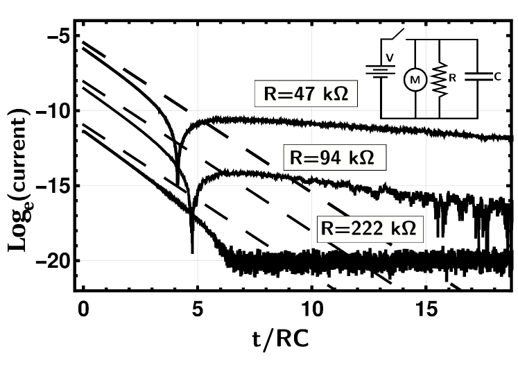
Figure 1: Decay data of $\log_{e}|I_{R}|$ for the circuit schematic shown in the inset. The air capacitor has $C=240$pF while $M$ is a voltmeter. The $R=47~{}\mathrm{k}\Omega$ trace is offset upwards on the y-axis while the $R=222~{}\mathrm{k}\Omega$ trace is offset downwards on the y-axis to avoid overlap of the traces. The dashed lines, illustrating the predictions of Kirchhoff’s laws, are offset slightly above the corresponding data. The dips in the graph indicate when the current switches direction.

III Constructing knowledge

Creating knowledge about this circuit can be classified into two parts. The first involves determining that the results are repeatable and known with certainty to reflect the behavior of the RC circuit; that is, establishing confidence that the results are valid. The second involves creating a model that the data support within error.

III.1 Establishing experimental validity

One method to determine data validity involves questioning the function and influence of each system component. For example, the switch not only disconnects the conducting path but thereafter it has an intrinsic capacitance. Since the switch bounces, bounce advanced triggering techniques are required to obtain repeatable data. The wire loop of the circuit generates a self-inductance and therefore an electromotive force during the decay. The capacitor response is often modeled as having capacitance, series resistance, and inductance, the effects of which need to be considered (self resonance typically occurs at frequencies above $100$ MHz murata ). The resistance varies with temperature, which is a function of the electrical power dissipated in the resistor (which is a function of time during the decay). The capacitor constricts as a function of voltage, thereby changing its value. The analog-to-digital converter behaves non-linearly at some level of accuracy. The input impedance of the oscilloscope scope probe loads the circuit. Aware of the potential influence of each of these system components, the student can at this point design experiments or perform calculations to determine the impact of these effects (none of which invalidate the data presented).

This RC laboratory exercise exposes students to experimental techniques that are needed to collect reliable and repeatable data. Examples are the advanced triggering of an oscilloscope needed to mitigate the effect of switch bouncing. In addition, the effect of the measuring instrument (input capacitance of the oscilloscope) on the circuits becomes important when using capacitors with small capacitance values or when measuring the voltage between capacitors in series (a large meter input impedance is needed to mitigate discharge through the meter from such a measurement). The use of circuits with time constants on the order of a fraction of a second allows voltage noise baselines on the order of microvolts in the measurement (using integration over a power line cycle that is provided as a feature in many voltmeters).

III.2 Constructing models

Aware of the discrepancy yet confident of the validity of their data, the student can now be guided by the instructor to construct new models to explain their observations.

III.2.1 Using analogical models

The student can be exposed to the use of analogical models in an attempt to provide insight into this circuit behavior. In this regard and in an effort to help the student make connections, the instructor may first challenge the student to suggest physical processes that exhibit exponential decay and then to consider how such decays may possibly be modified to exhibit the behavior shown in fig. 1. peshkin

III.2.2 Fundamental principles

The student should now clearly recognize that the physics curriculum is focused on understanding fundamental principles rather than on manipulating a litany of equations. When a novel phenomenon is encountered it is considered from the perspective of these principles; this emphasis on fundamental principles should stimulate questions associated with validity of these laws.

The RC decay is most often modeled using Kirchhoff’s and Ohm’s laws. This emphasis on fundamental principles should arouse curiosity about the validity of these laws. Although Ohm’s law is not fundamental it is expected to be appropriate in the analysis of the circuits described here, while Kirchhoff’s laws are strictly valid for steady state behavior.

In recognizing that the steady state regime may not be appropriate, the student might ask if the data reproduces Kirchhoff’s result for much larger time constants. Indeed, for the $222~{}\mathrm{k}\Omega$ resistor shown in fig. 1, the dip or change in current direction is eliminated while the decay better matches the exponential decay predicted by Kirchhoff’s law, although its tail still violates the prediction of exponential decay.

Kirchhoff’s laws are superseded by Maxwell’s equations. Only a few circuits, involving steady state behavior, have been treated in this manner analytically. sommerfeld ; heald ; chabay ; klee ; muller ; moreau Maxwell’s equations have been solved numerically for an RC circuit. preyer However, the data presented here do not support the results of that calculation.

The intent of this exercise is not for the student to develop a novel solution to RC decay using Maxwell’s equations, but rather to use this open ended problem as an example of how a physicist begins to make sense of such data. What often distinguishes an expert from a novice is knowing what to question in light of confounding data. The experimental results described above allow the instructor to awaken and further encourage such awareness.

III.2.3 Constructing models that eliminate all extraneous parameters

The essence of a problem can often be revealed by a model that eliminates all extraneous parameters (as illustrated by the spherical cow metaphor wiki ). The decay of an air capacitor provides a system where this approach can be fruitful.

Students can be asked to construct a model that eliminates all extraneous parameters in RC decay. As an example, they may consider replacing the air capacitor with a single spherical conductor (having only self capacitance) attached to ground (or to infinity) via a resistor through which the charge flows in the decay. This model eliminates the effect of the second plate on the decay and appears to contain the bare minimum number of components needed to generate RC decay.

Having established this thought experiment the student may focus on how to implement it: using the metal sphere available from a Van de Graaf demonstration apparatus, or soldering the terminals of the air capacitor together. A careful design is first required to determine feasibility, particularly since the capacitance of the measuring apparatus typically overwhelms the small self capacitance of the sphere or the capacitor with its terminals soldered together.

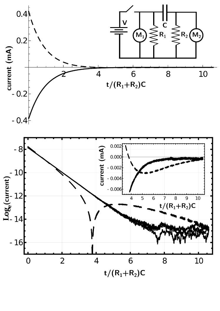
Figure 2: The decay currents through $R_{1}$ (dashed) and $R_{2}$ (solid) as a function of time. The circuit is shown in the upper inset. The results of four decays are superimposed. The inset is an expanded view of a portion of the data. $R_{1}=153~{}\mathrm{k}\Omega$ and $R_{2}=2~{}\mathrm{k}\Omega$ while the air capacitor has $C=240$pF.

To more accurately model the air capacitor the student may choose to add another spherical conductor, connected to ground through a different resistor, and brought near to the first spherical conductor. The system then has both self and mutual capacitance.

Such a revised thought experiment generates questions about the effect of the charges on one sphere attracting those on the other and thereby modifying the decay process, potentially causing the non-exponential decay in the air capacitor. The charges on one plate repel each other, leading to the voltage decay, while the opposite charges on the nearby plate counteract this decay.

The addition of this second spherical conductor may lead the student to the idea of connecting each plate of the air capacitor to ground via different resistors. One advantage of including another resistor in the circuit is that the voltage across each resistor reveals the currents flowing into or out of each capacitor plate. The student might then revise the experiment as shown in the circuit schematic of fig. 2.

III.2.4 Testing and refining the new model

A cursory examination of this data in the upper frame appears to support equal currents flowing into and out of the capacitor as expected from Kirchhoff’s law. The student may be tempted to go no further in their pursuit of experimental confirmation of the Kirchhoff model. However, when prodded to use a logarithmic scale, discrepancies are apparent, as shown in the lower frame of fig. 2. This illustrates the importance of attention to detail and how an improvement in the accuracy challenges a scientific model.

Again, the dip in the logarithm plot occurs when the current changes direction. Also, the current decay from the right capacitor plate monotonically decreases (and is initially exponential) while the current in the left plate switches direction and is similar to that shown in fig. 1. This is evidence for a time varying net charge on the capacitor. However, the initial charge is not measured with this circuit.

The student may choose a different modification of the single charged sphere model: placing a neutral isolated spherical conductor near to the charged spherical conductor. In this case the exponential decay of the latter is modified by the charges induced on the isolated sphere (rather than those drawn to the second sphere through its resistor connected to negative side of the battery). Perhaps the charge on the first sphere does not decay to zero due to the mutual attraction between it and the induced charges on this isolated sphere.

To test this the student might use two capacitors in series as shown in upper frame of fig. 3. The right plates are similar to the isolated sphere. By measuring the voltage across $R_{2}$ the current between the right plates is determined (such current data are not shown).

Initial net negative charge on the right plate of $C_{1}$ and no net charge on the right plate of $C_{2}$, in the upper frame of fig. 3, is generated when the two switches are closed. The decay is measured when these two switches are opened simultaneously (within a millisecond using a double pole single throw mechanical switch for a $338$ millisecond time constant). After the two switches open some of the charge on the right plate of $C_{1}$ relaxes to right plate of $C_{2}$. The voltage between the plates of $C_{2}$ decreases below its equilibrium value $V_{f}$, as shown in 3 (b) by the dashed line, before returning to it, illustrating behavior similar to that shown in fig. 1, even though the capacitor contains a dielectric with a capacitance four orders of magnitude larger than the air capacitor.

The more familiar initial condition for the series capacitor configuration results from removing the switch across $C_{2}$. For comparison the decay for this initial condition is shown in fig. 4.

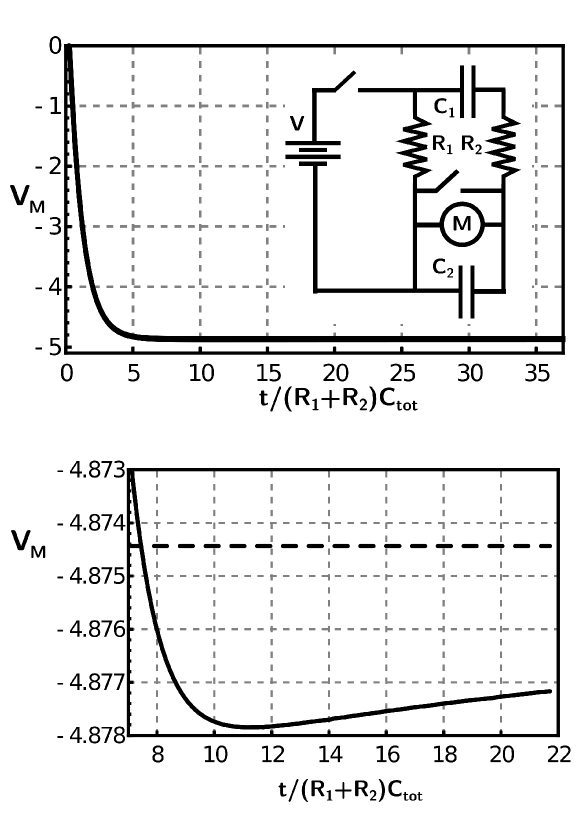
Figure 3: Voltage across $C_{2}$ for resistor values of $R_{1}=1~{}\mathrm{k}\Omega$ and $R_{2}=337~{}\mathrm{k}\Omega$ with capacitor values $C_{1}=C_{2}=C=2\mu$F (film metalized polypropylene axial capacitors) for the circuit shown in the inset of the upper frame. The two switches are initially closed to charge the circuit then open simultaneously. The dashed line indicates the final voltage $V_{f}$.

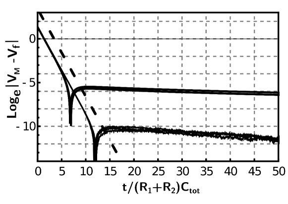
Figure 4: Plots of $\log_{e}|V_{M}-V_{f}|$ for the circuit in the upper frame of fig. 3. Four decays are are shown when the switch across $C_{2}$ is operational (the four upper traces that appear as one solid line) and when it is always open (the lower four traces).

The above data provide direction for constructing models. For fig. 1 the most obvious is $V_{M}=V_{10}\exp[-\alpha t]+V_{20}\exp[-\beta t]$ where $\alpha=1/RC$ and $\beta$ is the second decay constant after the dip. For fig. 3 this becomes $V_{M}=V^{in}_{f}(1-\exp[-\alpha t])+V^{out}_{f}(1-\exp[-\beta t])$ where $V_{f}=V^{in}_{f}+V^{out}_{f}$. This is referred to as the sum of exponentials model (fits of the data from a related circuit are found in the literature).kowalski

III.2.5 Validity of model parameters: dynamic capacitance

One aspect of modeling is determining the validity of the parameters used. Consider capacitance, for example. The assertion that the ratio of the charge to the potential difference is a constant can be tested with the circuit of fig. 1 by integrating the current leaving one capacitor plate to determine its remaining charge at a given time. Dividing this by the voltage across the capacitor at that time does not yield a constant value throughout the decay. Therefore, capacitance may not be a useful circuit parameter.

However, in modeling non-linear systems a connection is often made between a static parameter and its dynamic version. Examples are found in both static and dynamic resistance (applied to a p-n junction, that was perhaps discussed in an earlier course on electronics) and dynamic inductance (ferromagnetism is often discussed in a first year course). Even the relationship between phase velocity $\omega/k$ and group velocity $d\omega/dk$ (discussed in an earlier course on modern physics) is a similar quantity and its derivative.

Suggesting to the student that the dynamic capacitance $C_{dyn}=dQ/dV$ may be a useful parameter leads to the ordinary differential equation $C_{dyn}dV/dt=-V/R$. where $V$ is the voltage across the capacitor and $dQ$ the change in charge on the left plate of the capacitor in fig. 1. Kirchhoff’s law for this RC circuit is obtained from this relationship when $C_{dyn}\rightarrow C$ (for exponential decay $C_{dyn}=C$). Using this method a first order ODE has a solution that is a sum of exponentials. For example, $C_{dyn}$ can be determined using the expression for the voltage from the sum of exponentials model described above. The value of $C_{dyn}$ is then the capacitance measured by a capacitance meter for $t\ll RC$ that transforms into the much larger value associated with the $\beta$ relaxation time for $t\gg RC$.

III.2.6 Return to fundamental principles

It is surprising that the capacitor, whose dimensions do not change appreciably, can have a capacitance that varies as suggested by the dynamic capacitance model. This conundrum may stimulate the student to focus on acquiring a fundamental understanding of circuit behavior using Maxwell’s equations before addressing the data. Such solutions typically involve steady state behavior, utilizing a surface charge on a wire to confine its current. muller ; sommerfeld ; heald ; chabay ; moreau A numerical calculation involving relaxation in an RC circuit yields an initial non-exponential decay due to transit time effects but does not match the above data. preyer Surface charge effects are demonstrated with circuit wire that has a kink. If the current into the kink is greater than that out, “Then the charge piles up at the ‘knee,’ and this produces a field aiming away at the kink. The field opposes the current flowing in (slows it down) and promotes the current flowing out (speeding it up) until these currents are equal, at which point there is no further accumulation of charge and equilibrium is established.” griffiths2

Drawing an analogy between the charge on the kink and the capacitor in the circuit of fig. 1 the student may divide the charge into two parts: one that generates a field only between the capacitor plates, $Q^{in}$, that exerts no force on the current in the wires and one that confines the current to flow in the wires, $Q^{out}$. For example, before the switches are opened in the circuit of fig. 3, $Q^{out}$ generates zero electric field in the wire segment from the upper node along the branch to the capacitor while the field is non-zero in the segment from the upper node along the other branch to the resistor, thereby directing the current from the battery into $R$ and not to the capacitor. This is referred to as the sum of charges model. The response due to these charges is the sum of their individual responses from the superposition principle and is manifest as the first (given by the standard solution for the RC circuit) and second terms in the sum of exponentials model. Let the parameters of the second term be $Q^{out}_{0}=V^{out}_{0}\tau_{out}/R$, where $\tau_{out}$ is a constant and $V^{out}_{0}$ is the voltage at the plate generated by $Q^{out}_{0}$. The initial charge $Q^{out}_{0}$ is inversely related to $R$ in a manner analogous to the kink in the wire; larger charge is needed to redirect a larger current from the capacitor plate into the resistor. Support for this conjecture along with other examples of the sum of exponentials and sum of charges models (along with fits of the data) are found in the literature. kowalski

To vary the amount of $Q^{out}$ compared with $Q^{in}$ on a capacitor plate the student might modify the circuit in fig. 2 by adding a different voltage source, $V_{2}$, across $R_{2}$ using a switch that opens synchronously with the other switch. As $V_{2}$ approaches $V$ the field inside the capacitor is reduced (as is $Q^{in}$) while $Q^{out}$ on the plates has not been diminished (it is still required to direct current through the resistors). Data for such a modification are also found in the literature.kowalski

The sum of charges model attributes the unusual behavior of $C_{dyn}$ to the $Q^{out}$ charges on the capacitor (and the circuit wires) that are not included in the definition of capacitance, $C=Q^{in}/\Delta V$. Since $Q^{in}$ and $Q^{out}$ decay at different rates the capacity to hold charge at a given voltage is not constant.

III.2.7 Summarizing the new knowledge constructed

Consider the knowledge generated from the above process:

• Valid data for RC decay, obtained for both air and dielectric capacitors, indicate a change in current direction during the decay;

• At least two sequential relaxation mechanisms occur during the decay with disparate time constants. The first decay constant is that expected from Kirchhoff’s laws while the second is unrelated to the first;

• Unequal currents flow into and out of the capacitor in RC decay;

• Net charge is generated on the capacitor;

• The sum of exponentials model matches the observed behavior;

• The series capacitor circuit provides a method to explore how charge flows between isolated conductors during the decay;

• The use of dynamic capacitance in modeling this data is of limited utility since it does not present a microscopic understanding of the process and therefore has little predictive power;

• The sum of charges model supports the sum of exponentials model since the initial decay time constant, RC, is the same for all data sets while the parameters of the the second term in the sum of exponentials model need to be adjusted to match the particular decay. For example, $Q^{out}$ for the left plate in fig. 2 differs from that on the right plate in order for the sum of exponentials model to match the data from each plate, yet the initial decay term for both involve the time constant $(R_{1}+R_{2})C$.

• Before the switch is opened $Q^{out}$ directs current into $R$ while the electric field from $Q^{in}$ has no such influence since it is confined to a region between the plates (without $Q^{out}$ and before the switch is opened the student might ask what force causes current to flow through the resistor if the field from $Q^{in}$ does not exist in the wires to move charges);

• The description of transient behavior using a kink in a wire is related to the behavior of the capacitor and consistent with the sum of charges model;

• The decay of the circuit in fig. 2 with a different voltage source across each resistor (that initially energizes it) allows for a variation in $Q^{in}$ while $Q^{out}$ is essentially fixed, thereby facilitating tests of the sum of charges model. While progress has been made a microscopic understanding of the decay process, based on Maxwell’s equations, is absent.

As with any model questions arise that probe its consequences. The student may wonder about the effects of $Q^{out}$ in an inductor-resistor circuit, or about the consequences of the sum of charges model when the loss mechanism involves transfer of the electrical energy stored in the capacitor to mechanical energy or to other circuit components. Perhaps a superconducting LC circuit, whose loss mechanism is radiative rather than thermal, behaves in the same manner. On a theoretical level, they may wonder why the simple sum of exponentials model matches the data even though it is quite difficult to obtain such a solution from Maxwell’s equation.

Through this exercise, the student not only has experienced the process of constructing new knowledge, but also experienced the questions and uncertainties it often exposes.

IV Conclusions

Students in an upper-level undergraduate physics laboratory class can be effectively exposed to the process of constructing new knowledge in physics. This involves the acquisition of valid data along with the construction of models supported by the data within error. The simple RC circuit, for which accurate measurements can be made inexpensively, is surprisingly difficult to model on a fundamental level. Yet the physics involves the familiar attraction and repulsion between charges. The students should be cognizant of the learning objective: the point is to learn how to collect valid data, practice modeling, and think critically about the data supporting the models, not to find a unique model that the data support. Hopefully, joy can be found in this process rather than only in the result, for which complete success is often elusive.

This laboratory experience also provides an opportunity for students to become aware of the differences between the simplified models ubiquitous in their formal education and the more complex realities of the physical world. Not only do students gain fresh insight into how new knowledge is constructed, but they move toward a more mature and sophisticated view of physics.

V Appendix

The instruction described above is a fruitful but time intensive endeavor. Alternately, a shorter exercise described next saves considerable course time while still cultivating some skills essential for constructing new knowledge. This has been successfully implemented as a pre-post assessment in a junior level modern physics laboratory course.

Students are told that the purpose of the pre-test is to determine their skills in performing experiments and communicating their results. Rather than being given written instruction, they are simply told to use the equipment at hand to collect RC decay data and write a short scientific report on their work.

The data that they collect using a microfarad ceramic or electrolytic capacitor and a $1~{}\mathrm{k}\Omega<R<100~{}\mathrm{k}\Omega$ resistor with an 8-bit oscilloscope appears to match Kirchhoff’s law during the initial decay. However, its tail deviates significantly from exponential decay even when analyzed with an 8-bit resolution oscilloscope. In the pre-test many of the students conclude that this data indicates exponential decay, verifying what was taught in a previous class (many plot the data on a linear scale). A remarkable number of reports do not reflect an awareness that modeling is a fundamental part of a scientific method; that is, the reports lack an argument that the data support a model within error.

As a summative assessment later in the semester, the student repeats the experiment (or is given a file of decay data with unique RC values for each student to mitigate cheating). From this data the student writes a laboratory report. Learning in the course is illustrated as the student compares their pre-test and post-test documents. Although this alternate exercise saves considerable course time, it has the pedagogical shortcoming of not allowing the students practice in modeling and experimental design. Nevertheless, it has the advantage of challenging the student to think critically about the validity of the data, particularly in the case where the student expects the data to support the model within error. This is an important first step in constructing new knowledge.

References

- (1)
- (2) F. V. Kowalski, (in press) “Energy relaxation in a vacuum capacitor-resistor circuit: measurement of sequential decays with divergent time constants.”
- (3) ”Lumped Circuit Model”, https://www.electronicdesign.com/technologies/analog/article/21155418/logiswitch-11-myths-about-switch-bouncedebounce (Accessed: 2023-3-4).
- (4) ”Lumped Circuit Model”, https://www.electronicdesign.com/technologies/analog/article/21155418/logiswitch-11-myths-about-switch-bouncedebounce (Accessed: 2023-3-4).
- (5) Cadence, “Capacitor Self-resonant Frequency and Signal Integrity,” (2019), https://resources.pcb.cadence.com/blog/2019-capacitor-self-resonant-frequency-and-signal-integrity (Accessed: 2023-4-3).
- (6) It is temping to suggest that the quantum theory of decaying states is such an example. That is disputed in the following references: M. Peshkin, A. Volya, & V. Zelevinsky, Non-exponential and oscillatory decays in quantum mechanics. EPL (Europhysics Letters). 107, 40001 (2014,8), https://doi.org/10.1209/0295-5075/107/40001 and P. Greenland, Seeking non-exponential decay, Nature, 335, 298 (1988).
- (7) A. Sommerfeld, Electrodynamics. pp. 125-130 (1952).
- (8) M. Heald, Electric fields and charges in elementary circuits. American Journal Of Physics. 52, 522-526 (1984), https://doi.org/10.1119/1.13611
- (9) R. Chabay & B. Sherwood, Polarization in electrostatics and circuits: Computing and visualizing surface charge distributions. American Journal Of Physics. 87, 341-349 (2019), https://doi.org/10.1119/1.5095939
- (10) M. Klee, Surface charges from a sensing pixel perspective. American Journal Of Physics. 88, 649-660 (2020), https://doi.org/10.1119/10.0001435
- (11) R. Muller A semiquantitative treatment of surface charges in DC circuits. American Journal Of Physics. 80, 782-788 (2012), https://doi.org/10.1119/1.4731722
- (12) W. Moreau, Charge distributions on DC circuits and Kirchhoff’s laws. European Journal Of Physics. 10, 286 (1989,10), https://dx.doi.org/10.1088/0143-0807/10/4/008
- (13) N. Preyer, Transient behavior of simple RC circuits. American Journal Of Physics. 70, 1187-1193 (2002), https://doi.org/10.1119/1.1508444
- (14) “Spherical Cow,” https://en.wikipedia.org/wiki/Spherical_cow (Accessed: 2023-4-2).
- (15) D. J. Griffiths, Introduction to Electrodynamics: second edition, Prentice-Hall, pp 277–278 (1989).